Abstract
The seasonal variation in mixed layer salinity (MLS) plays a crucial role in global ocean circulation and hydrological cycle. The salinity budget of the mixed layer is important to understand the mechanism of the variation, but in the South China Sea (SCS), the details in the budget are missing due to insufficient observations. Here, we employed an eddy-resolving (horizontal grid resolution ~10 km) SCS circulation model to quantify the key physical processes in the seasonal cycling of MLS in the northern South China Sea (NSCS). Built on the success of the realistic numerical simulation for 2008–2018, the model reproduced the primary features of the observed seasonal MLS, wherein fresher waters are present in the region during the summer monsoon and salty waters appear along the slope during the winter monsoon. According to the salinity budget that was calculated during model execution, the term for air–sea freshwater flux and meridional advection represent the primary freshwater input in the summer and winter, respectively, while vertical processes including vertical mixing and entrainment form the major balancing terms in the budget. In different regions of the NSCS, vertical mixing can play a dominant role in the vertical processes, but the associated seasonality is different for regions of strong internal wave influence and regions of strong horizontal advection influence. In the winter, the intrusion and spreading of western Pacific water over the NSCS could modify the MLS structure and cause larger vertical entrainment than mixing in regions where the effect of mixing decreases with the slackening of the seasonal internal wave activities. Overall, the analysis of the ML salinity budget reveals that vertical mixing, together with vertical entrainment, is vital to maintaining the seasonal variation in MLS of the NSCS.
1. Introduction
The South China Sea (SCS) is the largest marginal sea in the tropics, with two extensive continental shelf areas in the north and south, and a basin in the center that is more than 3000 m deep (Figure 1). It is a region influenced by Asian monsoons such that the mixed layer salinity (MLS), which is driven by winds, precipitation, and ocean circulation of SCS, exhibits distinct seasonal variation [1,2]. Spatially, rivers import large amounts of freshwater into the ocean interior, including the Mekong River in the southwestern SCS, the Pearl River in the northern SCS, and the Red River in the Gulf of Tonkin (Figure 1a) [3,4]. Rainfall also has a spatial distribution that is associated with islands and high mountains, e.g., the increased rainfall on the western side of Luzon Island in the summer. In addition to the freshwater input, the water in the northern South China Sea (NSCS) is exchanged with the water from the East China Sea through the Taiwan Strait and the water from the western Pacific Ocean through the Luzon Strait [5]. The Kuroshio intrusion through the Luzon Strait brings large amounts of warm and saline water into the basin [6,7]. All these conditions lead to a complex spatial–temporal change in the MLS of the SCS.
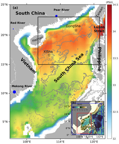
Figure 1.
(a) Geography of the SCS and the climatological SSS (shaded) during 2008–2018. The blue dots indicate the locations of major river mouths with the radius of each proportional to the magnitude of climatological freshwater outflow. The black box (15–23° N, 110–121° E) indicates the region of focus in the present study. The thin to thick gray contours represent the 100, 1000, and 3000 m isobaths, respectively. (b) The numerical model was set up in the blue box region (0.9–35° N, 99–135° E) with validations focused on the red box area (2–25° N, 105–122° E).
Recently, there have been several studies focusing on the salinity fields of the SCS based on either in situ measurements or satellite observations. For example, Yi et al. [8] used remote sensing data to analyze the multiscale variability of sea surface salinity (SSS) and the oceanic processes controlling the seasonality of SSS in the SCS. They noted more details are required to close the equations in diagnosing the MLS budget. Using an observational dataset, Zeng et al. [9] analyzed the subsurface salinity in the NSCS and revealed that the main processes controlling the subsurface salinity changes are horizontal advection and vertical entrainment processes. Zeng et al. [10] further analyzed the mixed layer salinity variability in the SCS for the period 1960–2015 and found that the observed trend in MLS can partly be explained by horizontal advection and vertical entrainment terms. However, the process of vertical mixing was ignored in the analyses.
The NSCS region features a strong vertical mixing that can result from various processes (e.g., internal wave and wind-induced mixing). The previous analysis of the MLS budget was difficult to balance since the observed data were insufficient to evaluate the vertical mixing term. As a consequence, vertical mixing is often treated as a residual term, potentially leading to large uncertainty or even an imbalance in the budget [11]. The lack of sufficient space and time coverage for the surface freshwater flux and the high-quality surface salinity data are the major limiting factors that prevent the processes governing the seasonal variability of MLS from being fully assessed.
Numerical ocean circulation models are extensively used to study the MLS changes in global [12,13] and tropical and subtropical regions, such as the Indian Ocean [14], the tropical Pacific [15], and marginal seas [16,17]. Compared to observations, a numerical model has the advantage of producing long salinity time series with high spatial and temporal resolution. Nevertheless, few studies of the MLS have been reported for the NSCS based on numerical models. In limited research, Yan et al. [18] investigated the summer low-salinity water west of Luzon. They found that rainfall was responsible for the formation of the low-salinity water, while Ekman pumping of high-salinity subsurface water during the northeast monsoon caused the low-salinity water to disappear. However, more numerical studies of MLS are needed to further understand the detailed processes of MLS variation and the driving mechanisms.
Following the analyses of Yi et al. [8] and Zeng et al. [10], in the present study, we investigate the details of SSS changes in the NSCS based on high-resolution numerical simulation results. Our focus is to evaluate the terms in the MLS budget that have been often ignored in previous studies. The estimations are prone to errors, including the terms of vertical mixing, vertical advection, and vertical entrainment. Compared to previous studies, a more comprehensive view of the NSCS seasonal MLS dynamics can be provided.
The paper is organized as follows. Section 2 provides a brief overview of the model setup, the equations of the mixed layer salinity budget, and the model validation datasets. In Section 3, we validate the simulation using available observations. Section 4 examines the processes that control the seasonal cycle of MLS, with particular attention being given to three selected regions in the NSCS that exhibit distinct MLS seasonal variability. Finally, we discuss our findings in Section 5 and provide a summary in Section 6.
2. Data and Methods
2.1. Model Setup
The numerical simulation was conducted using the Coastal and Regional Ocean Community (CROCO) model (https://www.croco-ocean.org/, accessed on 1 May 2022). It is a model system built upon the ROMS [19,20], and the latter has wide application in a diverse range of studies from estuarine and coastal scales to basin scales [5,21,22].
The model had a domain (0.9–35° N, 99–135° E) that not only includes the SCS but also the East China Sea and the West Pacific Ocean. The horizontal grid resolution was 0.1°, sufficient to resolve the lateral water exchange through the straits that connect the SCS with the surrounding waters (Figure 1). Vertically, the model had 31 levels distributed according to a stretched and generalized terrain-following sigma coordinate that was weighed toward the surface to better resolve the mixed layer and thermocline (with no less than 9 levels in the upper 100 m). The bathymetry data used in the model were ETOPO2 and smoothed slightly to reduce the terrain gradients and truncation errors.
There are three open boundaries set at the south, north, and east sides of the model domain, respectively (Figure 1b). Both tidal forcing and low-frequency variations were added to the boundary grids. The tidal forcing was obtained from a global barotropic tidal model (TPXO8) with 1/30° horizontal resolution. Eight major tide constituents including four semidiurnal frequencies (M2, S2, N2, K2) and four diurnal frequencies (K1, O1, P1, Q1) were used. The subtidal daily variations were obtained from the HYCOM reanalysis data during the time between 2008 and 2018. For the sea surface elevation and barotropic momentum the open boundary used the Chapman condition, and for other quantities (i.e., baroclinic momentum and tracers) the open boundary used the Orlanski radiation condition with the information of inflow enforced through nudging.
The model was initialized on 1 January 2008, with the temperature, salinity, sea surface height, and the eastward and northward velocity derived from the HYCOM reanalysis dataset. The simulation was from January 2008 to December 2018, and the period between January 2012 and December 2018 was chosen for analysis. The atmospheric forcing, including the 3-hourly wind velocity at 10 m, net shortwave radiation, downward long-wave radiation, air temperature at 2 m, sea level air pressure, specific humidity, and precipitation, were from the 0.25° ERA5 reanalysis dataset provided by the European Center for Medium Range Weather Forecast (ECMWF). In the model, the daily mean discharges of the Pearl River and the monthly mean discharges of the other 13 rivers (e.g., the Yangtze, Honghe, and Mekong), were used as freshwater point sources. Being a realistic numerical simulation, we apply no relaxation of the SSS to observations.
2.2. Equation of the Mixed Layer Salinity Budget
The mixed layer depth (MLD) is defined as the shallowest depth of the maximum buoyancy within the water column [23]. The governing equation for the salinity budget in the MLD can be written as follows, according to [16]:
where <·> denotes the vertical average over the mixed layer depth h. S is the salinity and (u, v, w) are the horizontal and vertical components of ocean currents. is the lateral diffusion operator, is the vertical diffusion coefficient, E is the evaporation, and P is the precipitation. The terms YADV and XADV represent the meridional and zonal advection, and the term VADV represents the vertical advection. ENTR and VMIX are the vertical entrainments and the vertical diffusion terms, respectively, through the mixed layer base. SF is the air–sea freshwater flux forcing of the mixed layer, and HMIX is the lateral diffusion. To obtain the mixed layer salinity budget, the terms in Equation (1) that contribute to the MLS evolution were computed online and saved on a 3-day average during the model simulation. We use this salinity budget calculation to infer the physical processes involved in the seasonal MLS evolution in the NSCS.
2.3. Validation Datasets
The sea surface salinity optimum interpolation product (OISSS) of NASA observations was used to validate the modeled SSS. The dataset (available for download at http://apdrc.soest.hawaii.edu/dods/public_data/satellite_product/OISSS, accessed on 11 November 2022) has a 0.25-degree grid resolution and a 4-day interval since September 2011. The dataset has been successfully used to study the linkage between observed SSS variability and the hydrological cycle [8].
The surface freshwater flux is important for SSS variability and needs to be validated in the model. Here, we used evaporation (E) from the Objectively Analyzed Air–Sea Fluxes (OAFlux) project [24] and precipitation (P) from the Tropical Rainfall Measuring Mission (TRMM) [25] to estimate the observed air–sea freshwater flux. The climatology of surface currents to assess the modeled circulation was derived from the Ocean Surface Current Analysis Real-time (OSCAR) project [26]. Additionally, we used the Argo T/S profiles to assess the vertical T/S structure in the model. The Argo profiles are for the period from January 2012 through to the end of the simulation (a total of 4678 profiles).
2.4. Model Skill
Agreement between the model and observations was evaluated quantitatively. According to [27], the model skill is defined as:
where Xmodel and Xobs are the modeled and observed variables, respectively. The “” means the average value of the variable for comparison. A perfect agreement between the model results and observations will yield a skill of one and, accordingly, a complete disagreement yields a skill of zero.
RMSE is a measure of how close the simulated value is to the observed one and is defined as:
where n is the total number of samples and X is the observed and simulated variable.
3. Model Validation
Strong seasonal patterns, namely the winter and summer patterns, dominate the variability of SCS since the local climate is predominantly influenced by the monsoon system [28]. The winter monsoon prevails from November to April and is characterized by cold and dry northeasterly winds that lead to a cyclonic upper ocean circulation in the SCS basin [29]. In contrast, the summer monsoon (mid-May to mid-September) is characterized by weaker southwesterly winds that induce a double-gyre circulation over most of the SCS [3].
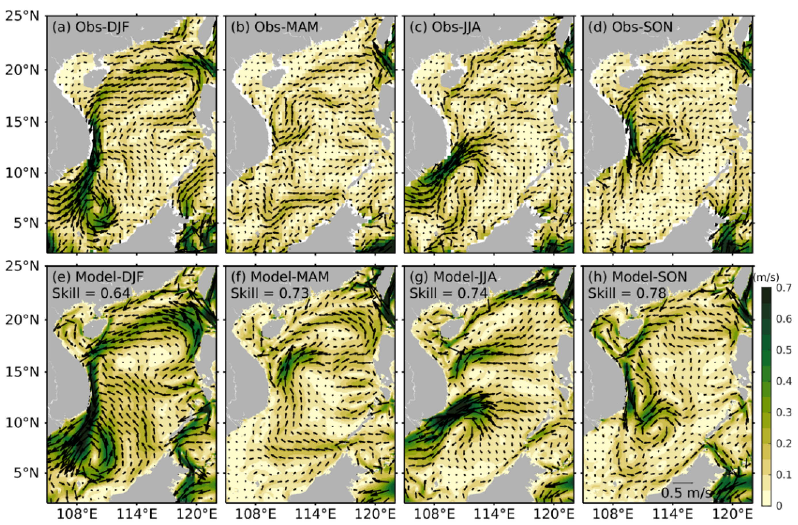
Seasonal climatology of the surface currents from the observed (OSCAR) and simulated data are presented in Figure 2. The monsoon-driven surface current patterns of the SCS are evident both in the model and observation. After the onset of the northeast monsoon (December–February), there is a strong westward flow in the central region of the NSCS, namely the South China Sea Upper Circulation (SCSUC) [29,30]. South of 18° N, the flow turns toward the equator along the west coast of the basin (Figure 2a). During the summer monsoon (June–August), there is a reversal of the SCSUC. It is characterized by a strong offshore jet at the southeast corner of the Vietnam coast (Figure 2c). The surface currents are weaker during the monsoon transition seasons (Figure 2b,d).
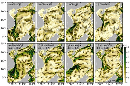
Figure 2.
The observed (a–d) and simulated (e–h) climatological surface currents in the SCS for the winter (DJF), spring (MAM), summer (JJA), and autumn (SON), respectively. The climatology is defined as over the period 2012–2018.
As shown in Figure 2, the model simulation slightly overestimates the observed surface velocities, particularly in the northwestern Luzon Strait during the winter (Figure 2e), and along the west coast of Vietnam where the overestimation is less than 20% (Figure 2a,e). Nevertheless, the model reproduces the observed spatiotemporal variation reasonably well with a skill of more than 0.74 (Figure 2g). In contrast, the model has a higher skill during the monsoon transition season (Figure 2f,h). Notably, the model effectively captures the timing of the SCSUC reversal.
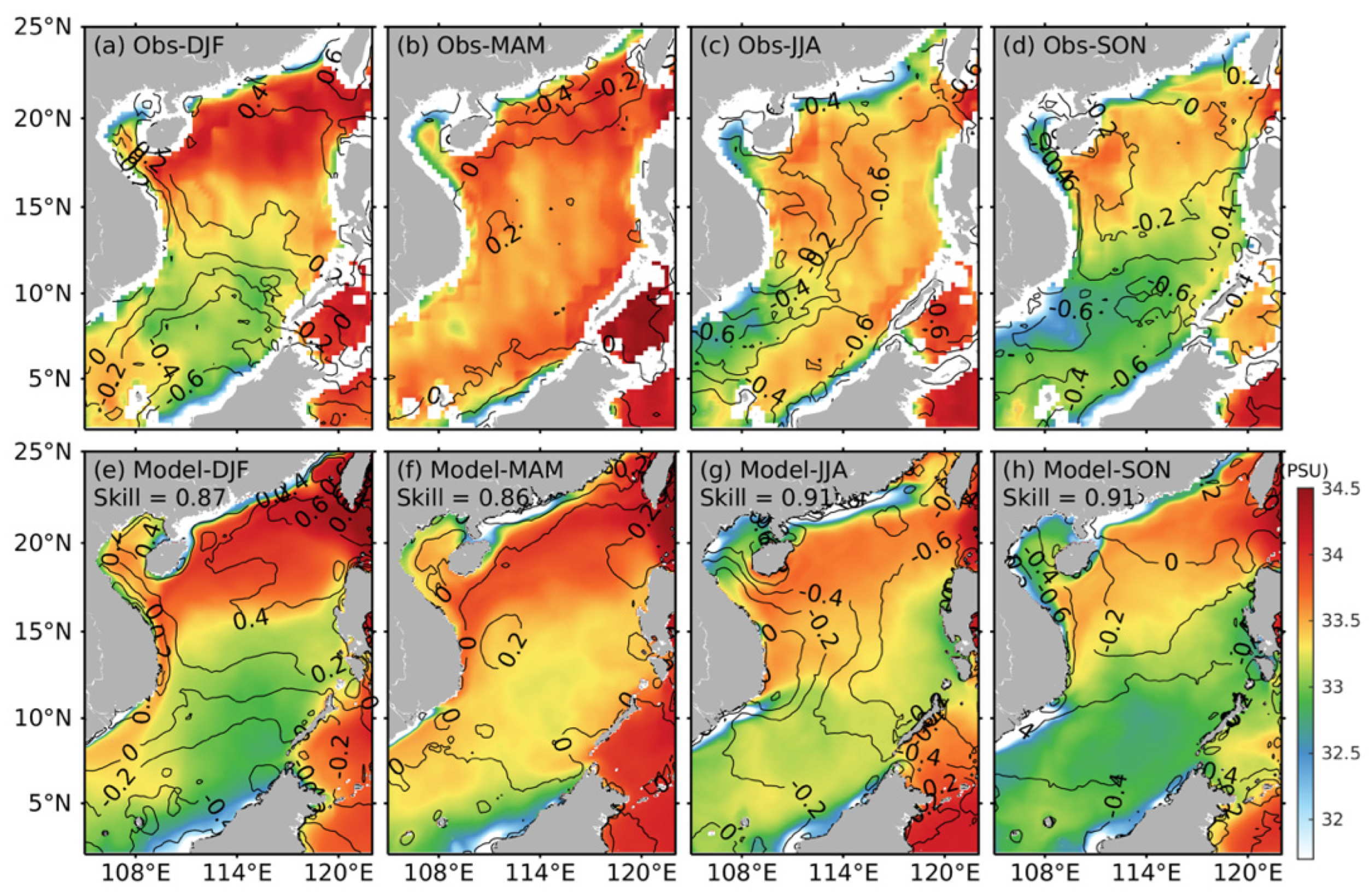
Figure 3 compares the climatology of modeled and observed SSS at different seasons. During the winter monsoon (December–February), high values of SSS (>34 PSU) appear in the northern part of the SCS (>15° N) as a result of Kuroshio water intrusion (Figure 3a). Surface freshwater flux (E-P) also greatly affects the NSCS SSS. There is a strong positive E-P flux up to 0.4 cm/day near the west of the Luzon Strait. During the summer monsoon (June–August), the SSS in the central basin is ~33.5 PSU due to the freshening effect of negative E-P fluxes as low as ~−0.6 cm/day (Figure 3c). At the same time, there are much smaller SSS values near the Pearl River and Mekong River deltas suggesting a contribution from the river runoff (Figure 3c). In contrast, there is a spatially more uniform distribution of SSS in the spring (Figure 3b) and autumn seasons (Figure 3d). Specifically, the SSS is around 33.5–34.0 PSU in the spring associated with a small positive E-P flux of less than ~0.2 cm/day. Autumn is the freshest season (~33 PSU) in the SCS. There is a small negative E-P flux of ~−0.2 cm/day in the NSCS but heavy rainfall and strong Mekong River runoff in the southern basin.
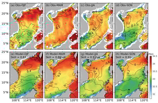
Figure 3.
The observed and simulated climatological SSS (shaded) and the climatological air–sea freshwater flux (E-P) (contour) in the SCS for (a) winter (DJF), (b) spring (MAM), (c) summer (JJA), and (d) autumn (SON), respectively. The contour interval is 0.2 cm/day. (e–h) for simulated.
The model simulation reproduces the observed SSS variation with a skill of more than 0.86. The relatively larger difference between the model and observation, particularly in the western Luzon Strait during the winter and autumn (Figure 3a,d), may be due to a slightly higher E-P flux in the model input from the ERA5 datasets. Nevertheless, the model effectively captures the timing of SSS evolution, and the slight overestimation does not affect the seasonal cycle of SSS in the SCS.
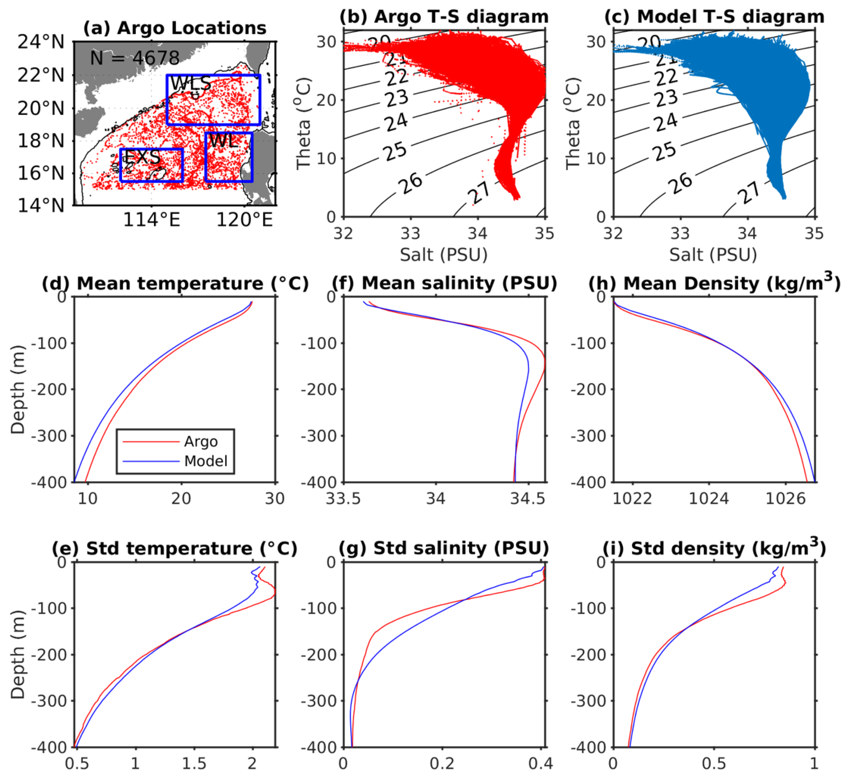
Figure 4a shows the distribution of Argo profiles selected for model validation. The resulting temperature–salinity (T-S) diagram is presented in Figure 4b and compared with the one derived from the model result (Figure 4c). The agreement between the model and Argo data demonstrates that the simulated T-S signature of the surface and subsurface waters resemble the observations in both space and time.
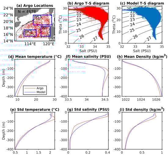
Figure 4.
Comparison of the temperature–salinity–density profiles between the Argo observations and model result. (a) Locations of the Argo floats (red) in the NSCS. The three boxes (blue) are selected regions for MLD validation shown in Table 1. (b) T-S diagram from the observations. (c) T-S diagram from the model. (d) Mean profile of temperature derived from the Argo and model data. Panels (f,h) are the same as (d) but for salinity and density, respectively. (e) Standard deviation anomaly of temperature profile derived from the Argo and model data. Panels (g,i) are the same as (e) but for salinity and density, respectively. The observation consists of 4678 profiles from 2012 to 2018.
The mean and standard deviation of the Argo-observed temperature, salinity, and density profiles are also displayed in Figure 4. The simulated temperature and salinity have an RMSE of 0.81 °C and 0.06 PSU with the observation, respectively. The model faithfully reproduces the vertical structure of these mean quantities (Figure 4d–i). But a mismatch in temperature (maximum of 1.17 °C at 400 m depth) and salinity (maximum of 0.09 PSU at 150 m depth) is observable. In addition, the model significantly underestimates the near-surface variability in temperature and salinity and overestimates the variability of salinity within the depth range 100–250 m. The underestimation may partly result from the inability of the model to resolve small-scale processes at a finer grid resolution. Additionally, differences in the subsurface variability between the model and observations may come from the Argo floats, which were sampled at a higher frequency.
Finally, the MLD is a key variable in the MLS budget analysis. Here, we present a validation against the estimation derived from the Argo data. As shown in Table 1, the model underestimates the MLD compared to the observations. The resulting biases and root-mean-square errors are moderate, approximately equal to the surface model layer thickness. The obtained skills justify the use of the model to reproduce the MDL both spatially and temporally.

Table 1.
Statistics of the Argo MLD (m) and model MLD (m) in the selected three box regions shown in Figure 4.
4. Results
4.1. Seasonal Variation in the Mixed Layer Salinity
4.1.1. Basin-Scale Features
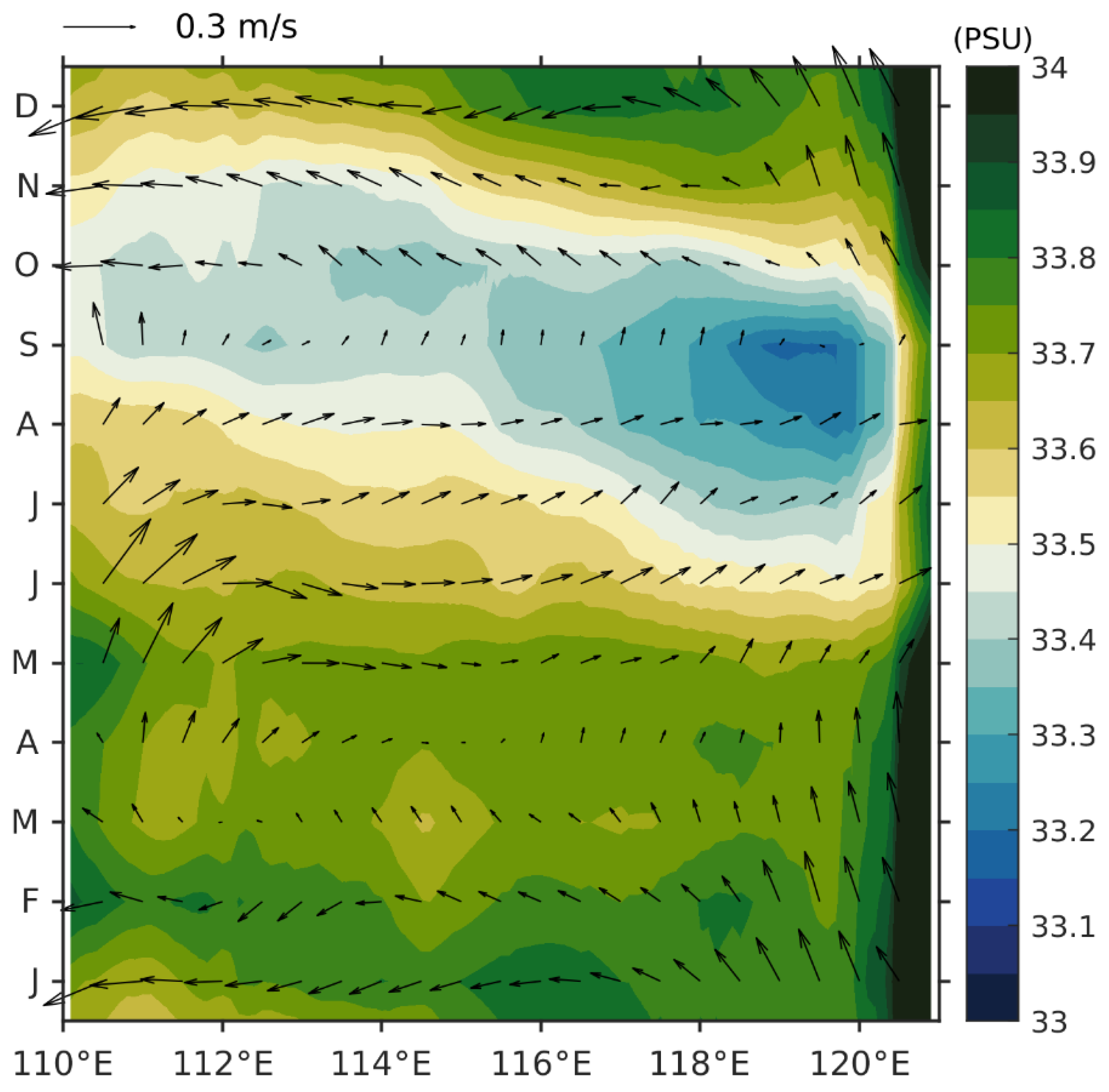
The seasonal variation in MLS for the region outlined by the box shown in Figure 1a was investigated and the longitudinal average of the result is shown in Figure 5. During the summer, the basin experiences a significant reduction in SSS (as low as 33.2 PSU). The freshening concentrates in the eastern basin and reaches a peak in August–September. In contrast, the freshening in the western basin is relatively weaker and has a one-month delay. From October to February of the following year, the basin-scale MLS quickly increases, starting from the eastern boundary of the basin. Between March and May, the basin exhibits the least zonal difference in MLS.
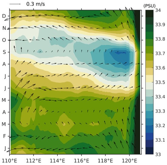
Figure 5.
The seasonal cycle of model SSS (shaded, PSU) and surface current (vectors, m/s) that are averaged over latitude in the box region of NSCS shown in Figure 1a.
The time–longitude analysis suggests that the eastern basin has a higher seasonal variation in MLS than the western basin. In the summer, the heavy rainfall on the western side of Luzon Island is responsible for the abrupt drop in the local SSS. In the winter, there are saline waters at the eastern boundary of the basin that come from the Pacific due to the Kuroshio intrusion through the Luzon Strait. It takes about 3–4 months for the westward zonal currents to spread the changes over the entire region (Figure 5).
4.1.2. Model SSS at Selected Regions
Figure 6a shows the standard deviation of monthly SSS that is produced by the model during the period 2012–2018. According to it, three subregions of the NSCS were selected for analysis, each having a different feature of seasonal MLS variation. The western Luzon Strait (115.0–121.0° E, 19.0–22.0° N; hereafter, WLS) is a region with the highest SSS variability. The intrusion of Kuroshio current through the strait determines that it is also a region with the highest seasonal MLS (Figure 6b). Western Luzon Island (117.5–120.5° E, 15.5–18.5° N; hereafter, WL) is a region also characterized by high SSS variability. However, it has the lowest summer MLS associated with the local strong seasonal rainfall (Figure 6c). The region of eastern XiSha (112.0–116.0° E, 15.5–17.5° N; hereafter, EXS) is the weakest in the seasonal SSS variation (Figure 6d).
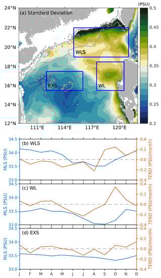
Figure 6.
(a) Standard deviation of monthly SSS from the 2012–2018 simulation. The blue boxes show the WLS, WL, and EXS regions. The 100 m and 1000 m isobaths are indicated by gray lines. The seasonal variation in mixed layer salinity is shown in (b–d) for WLS, WL, and EXS, respectively. The corresponding tendency of MLS is calculated based on the model output for the terms in Equation (1).
4.2. Mixed Layer Salinity Budget
The seasonal variation in the basin-scale MLS budget is discussed. For brevity, the zonal advection XADV, meridional advection YADV, and horizontal mixing HMIX are summed to represent the horizontal processes in the budget. The term HMIX for lateral diffusion is much smaller than the horizontal advection terms. Thus, its relative contribution to the horizontal processes can be ignored. Similarly, the vertical advection VADV, vertical entrainment ENTR, and vertical mixing VMIX are summed to represent the vertical processes in the budget.
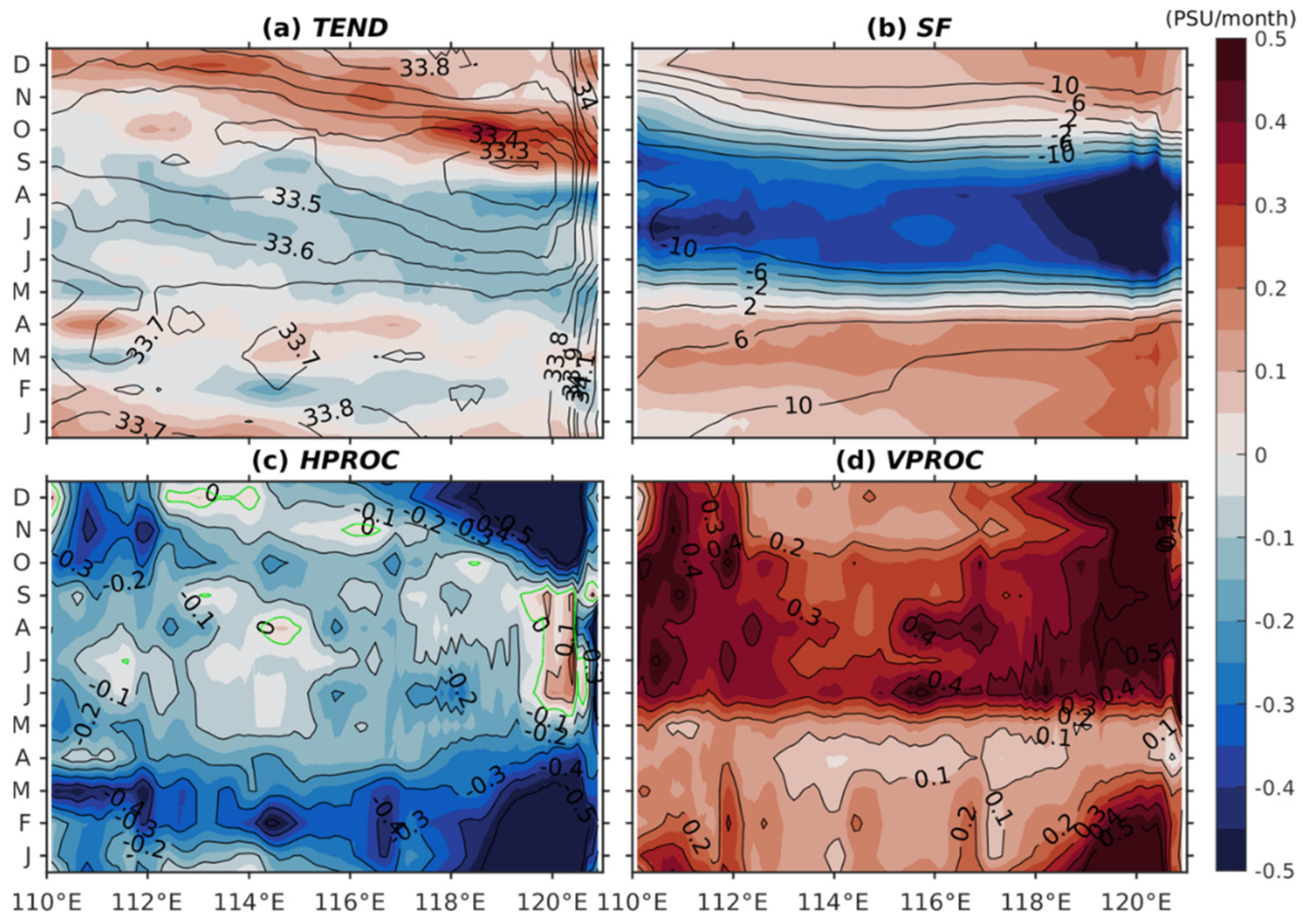
As shown in Figure 7, the term for air–sea freshwater flux and those representing the horizontal and vertical processes in the salinity budget all lead to an annual cycle of the basin-scale MLS. During the summer, the tendency of MLS reduction is strongly driven by precipitation, albeit a much smaller contribution can be seen from the horizontal processes. The vertical processes then take the role of balancing the surface freshening tendency. From October to February of the following year, the role of air–sea freshwater flux becomes opposite in the budget. The surface freshening, which is thus caused by the horizontal processes, remains small except in the eastern basin where the salination effect due to Kuroshio intrusion can be overwhelmed. As a consequence, both the atmospheric forcing and the vertical processes enforce a tendency for the basin-scale MLS increase. It is worth noting that the vertical processes always represent a dominant mechanism in the budget to balance the surface freshening tendency except between March and May when the vertical processes in the basin turn to be significantly weaker. During this period, the horizontal processes and evaporation can alternatively control the variation in MLS.

Figure 7.
The longitude–time plot of the major terms in the basin-scale MLS budget: (a) total tendency (TEND), (b) air–sea freshwater forcing (SF), (c) horizontal processes (HPROC = HADV + HMIX), and (d) vertical processes (VPROC = VADV + VMIX + ENTR). Contours in (a,c,d) are the surface salinity (PSU). The contours in (b) are the air–sea freshwater flux (E-P) (cm/month). See Equation (1) for the definition of each term in the salinity budget.
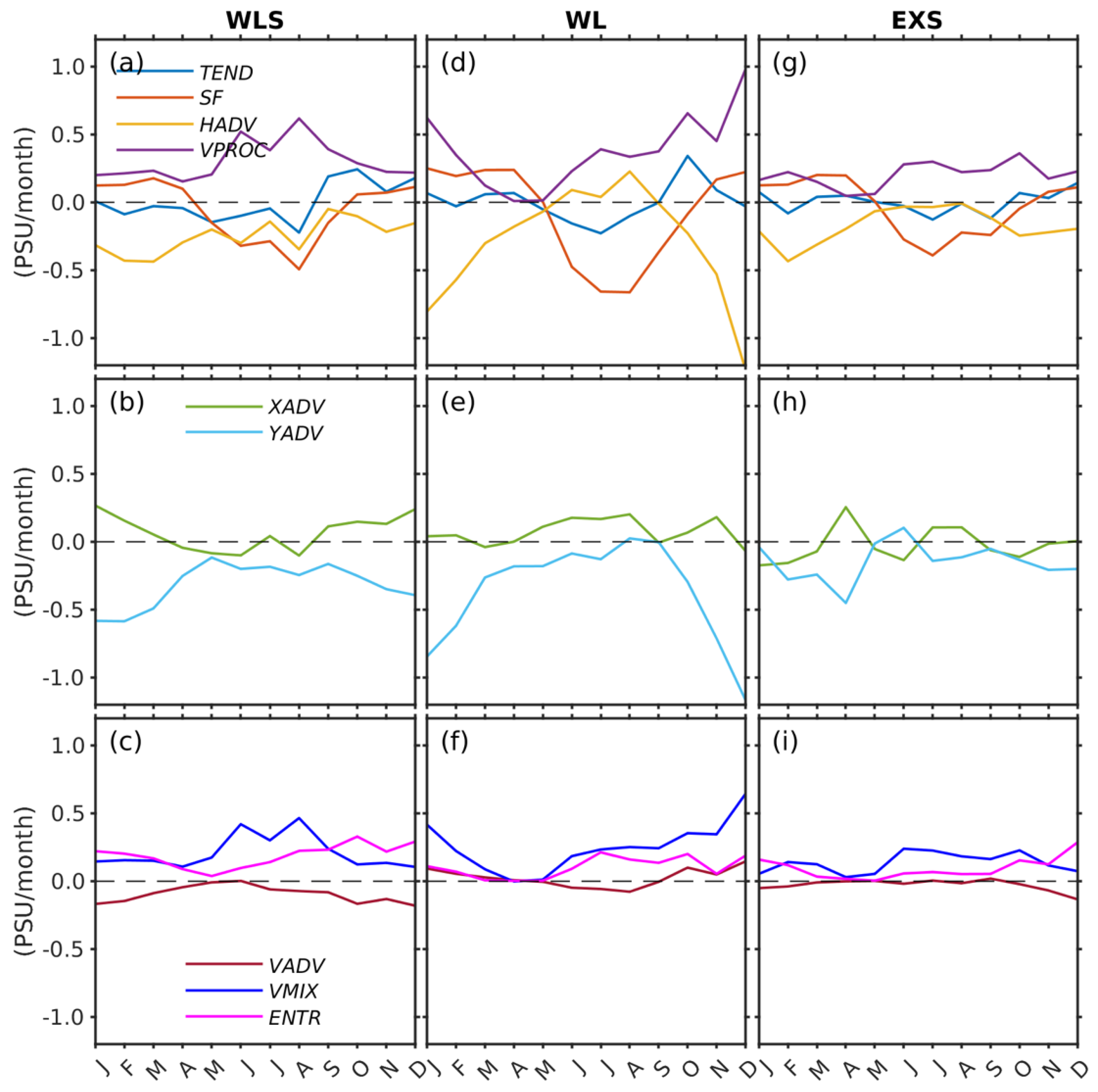
Figure 8 illustrates the MLS budget for the selected three regions. Compared with the basin-scale result, the seasonal variation in MLS in the local regions is also jointly controlled by the term for air–sea freshwater flux and those representing the horizontal and vertical processes in the salinity budget. But the balance details are regionally different and this spatial difference deserves further investigation.
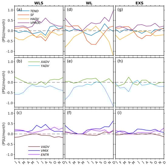
Figure 8.
Top panel: the seasonal variation in the major terms in the MLS budget for the (a) WLS, (d) WL, and (g) EXS regions. Middle panel: the seasonal variation in the major terms in the horizontal processes for the (b) WLS, (e) WL, and (h) EXS regions. Lower panel: the seasonal variation in the major terms in the vertical processes for the (c) WLS, (f) WL, and (i) EXS regions.
4.2.1. Western Luzon Strait (WLS)
The monthly salinity budget of this region is shown in Figure 8a. In the summer, the MLS reduction is strongly driven by precipitation. The contribution of horizontal processes to freshen the surface water is moderate during this period. In contrast, the vertical processes that bring underlying saltier water into the surface layer are strong too, and represent the key balancing term in the salinity budget to counteract the surface freshwater input. In the fall (September–November), the significant increase in MLS is driven by the vertical processes which at the same time are associated with the decrease in precipitation and the increase in evaporation. In the winter, all the terms in the salinity budget remain small except those representing the horizontal processes. Despite the Kuroshio intrusion, the total effect of horizontal processes can only lead to a freshening of the surface water, which is then balanced by evaporation and the vertical processes.
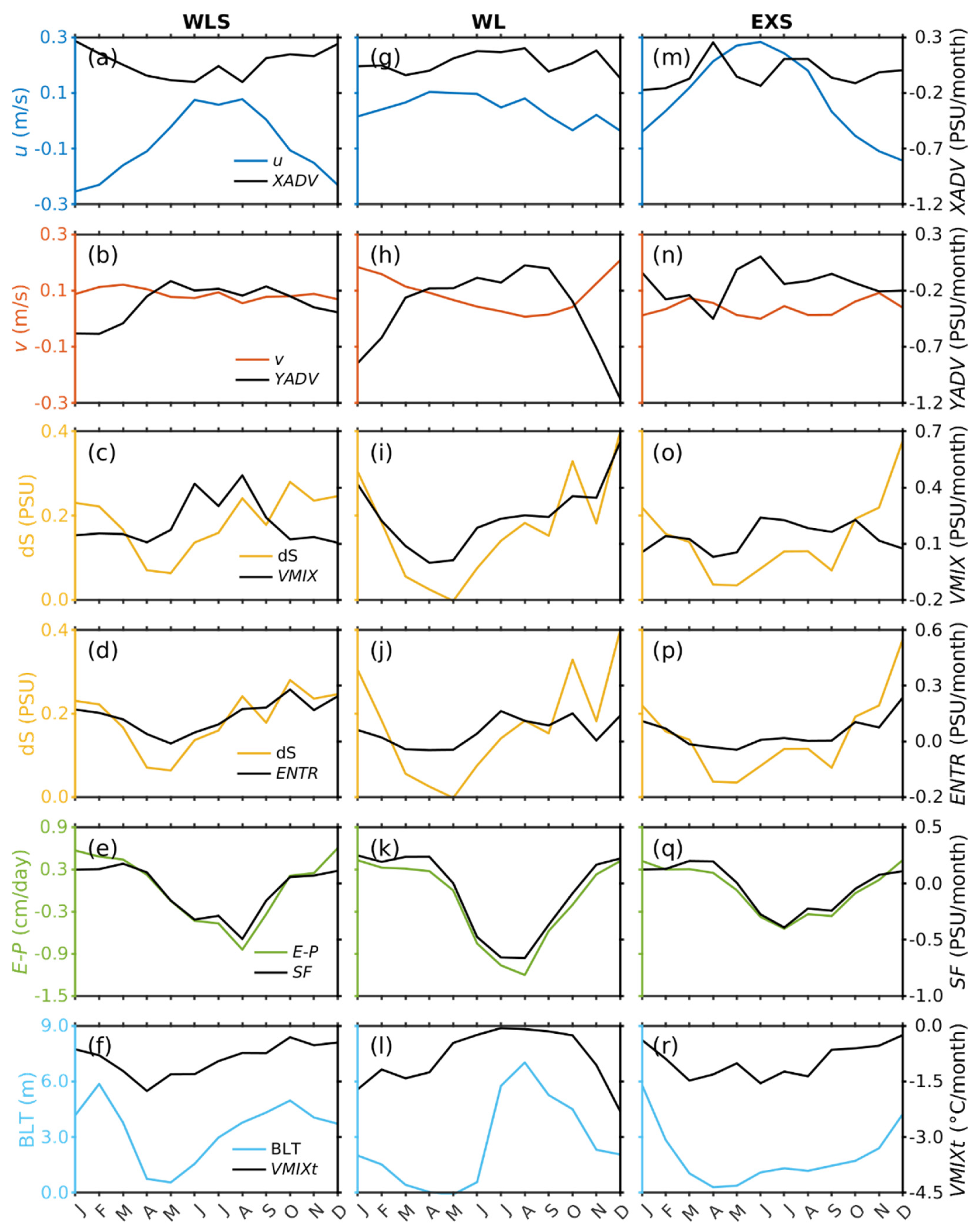
As evident in Figure 8b, the freshening of surface water from horizontal processes is a remote effect associated with the meridional advection of freshwater from lower latitude regions, e.g., WL. In the summer, this term is comparable in magnitude to the air–sea freshwater flux. In the winter, there is an even larger contribution from this term. According to Figure 9b, the meridional currents of WLS do not show a seasonal variation. The enhancement of horizontal freshwater advection, therefore, is determined by latitudinal salinity difference. To verify, one can see in Figure 3 that the latitudinal salinity difference is the largest in the winter season.
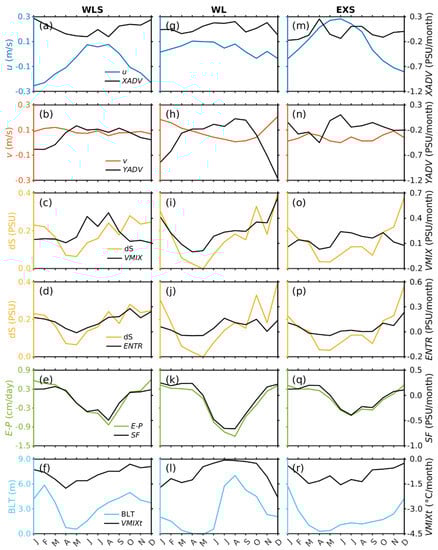
Figure 9.
The seasonal variation in the major terms in the MLS budget and the seasonal variation in the relative variables in the estimations for the three regions (WLS, WL, and EXS): (a,b) Seasonal evolution of the average model zonal/meridional horizontal advection term and zonal/meridional current over the WLS box. (c,d) Vertical mixing/entrainment term and salinity below mixed layer depth minus SSS. (e) Air–sea freshwater forcing term, freshwater flux E-P. (f) Mixed layer temperature vertical mixing term and barrier layer thickness. Panels (g–l) are for the WL region and (m–r) for the EXS region.
In WLS, vertical mixing is a dominant term in the vertical processes and exhibits a similar seasonal variation to the air–sea freshwater flux (Figure 8c). However, the seasonal variation in vertical mixing does not follow the corresponding seasonal variation in the vertical salinity difference (Figure 9c). Therefore, by increasing the vertical salinity difference between that in the mixed layer and just below, surface freshening appears not to be the key driver in the strong vertical mixing flux. Given that the WLS is a region characteristic of strong internal wave activities, the seasonality may alternatively be driven by the seasonal variation in internal wave-induced background turbulent mixing.
Finally, the term for vertical entrainment becomes important in the vertical processes during the winter. Figure 9d suggests that the vertical entrainment has a seasonal variation that is closely dependent on the vertical salinity difference. In the winter, the larger vertical difference in salinity may be a consequence of enhanced meridional advection of freshwater (Figure 8b).
4.2.2. Western Luzon (WL)
The monthly salinity budget in this region is shown in Figure 8d. The air–sea freshwater flux is the largest and causes a strong freshening of the surface water in the summer. The contribution of horizontal processes to freshen the surface water, however, is the smallest during this period, leaving the vertical processes as the major balancing term in the salinity budget to counteract the surface freshwater input. In the fall (September–November), there is a significant increase in MLS that is again driven by vertical processes and by the decrease in the air–sea freshwater flux. Since August, the role of horizontal processes in the salinity budget increases dramatically. The same is true for the vertical processes. Thus, the winter salinity budget is mainly between the horizontal and vertical processes.
In WL, the seasonal cycling of the salinity budget is different from that in the WLS. It is characteristic of strong freshwater input in the winter and is associated with the horizontal process that transports fresher water northward (Figure 8e and Figure 9h). However, the freshening of surface water is most significant in the summer. The winter freshwater input, although relatively larger, can be balanced by the vertical processes and induced salinity increase. Therefore, the local salinity budget also features a strong vertical process in the winter. However, the associated mechanism should be different compared to that in the WLS because it occurs in the winter instead of the summer.
One can see in Figure 8f that vertical mixing is still a dominant term in the vertical processes. However, the seasonal evolution of vertical mixing is similar to the vertical entrainment and follows the seasonal evolution of the vertical salinity difference between that in the mixed layer and just below it (Figure 9i). Since the subsurface salinity varies much less than the SSS at seasonal timescales, the term for meridional advection can be a good proxy for vertical mixing in the winter.
4.2.3. Eastern XiSha Island (EXS)
In EXS, there is a similar seasonal feature of the salinity budget to its eastern counterparts (Figure 8g). Generally, the air–sea flux and horizontal advection term represent the major freshwater input in the summer and winter, respectively. The term for vertical processes drives the MLS to increase all the time. Vertical mixing, again, is the dominant term in the vertical processes during the summer. According to Figure 9o, it should be more relevant to the seasonal variation in internal wave-induced background turbulent mixing. Overall, the comparison between the western and eastern basins reveals a weaker horizontal advection and less vertical mixing in the local salinity budget, which therefore leads to a smaller seasonal MLS variation.
5. Discussion
The analysis of the ML salinity budget suggests that vertical mixing, together with vertical entrainment, is vital in maintaining the seasonal variation in MLS in the NSCS. In WLS and EXS, the propagation and breaking of internal waves excited from the Luzon Strait provide strong background turbulent mixing in the summer and lead to a significantly larger vertical mixing than vertical entrainment in balancing the surface freshwater input. In the winter, the effect of vertical mixing decreases with the slackening of seasonal internal wave activities. At the same time, the intrusion and spreading of western Pacific water over the NSCS instead modify the MLS structure and cause a larger entrainment than vertical mixing. In contrast, the WL region has a different mechanism of vertical mixing. It is similar to the seasonal variation in vertical entrainment and associated with the vertical salinity difference between that in the mixed layer and just below it. In the winter, the greatly enhanced meridional advection brings in abundant fresher water from lower latitude regions. As a consequence, the vertical salinity difference enlarges and drives the increase in vertical mixing to balance the surface freshwater input.
Our results align with the findings of previous research [8,10], but we provide more details on the seasonal ML salinity budget of the NSCS. The term for vertical mixing is found important temporally and associated with different mechanisms spatially. This vertical flux was often ignored previously in both observational [31,32,33] and modeling [34,35] studies. We show that its magnitude can be significantly larger than vertical entrainment if associated with internal-wave-induced background turbulent mixing or other processes. Yi et al. [8] pointed out that the balance of seasonal SSS in the SCS seems to be very delicate, although atmospheric freshwater flux variation and horizontal advection could partly explain the seasonal variation in SSS, and that all the terms in the MLS budget need be considered. Zeng and Wang [11] confirmed that the summer low salinity water of WLS is caused by local freshwater fluxes; however, the residual term is large due to a lack of the vertical mixing term. Therefore, vertical mixing is a dominant term in the vertical processes and should play a decisive role in the closure of the balance.
Moreover, the important role of vertical processes in the ML salinity budget can have a profound influence on vertical temperature mixing at the bottom of the ML. Specifically, the presence of a barrier layer due to the depth difference between the surface isothermal layer and the salinity-relevant MLD may cause a weak vertical temperature gradient or a vertical temperature inversion, which prevents mixing from below the ML to affect the surface layer. In the NSCS, the term for vertical temperature mixing of the ML shows a seasonal variation that is completely different from that for vertical salinity mixing (Figure 9f,l,r). Instead, it closely follows the seasonal variation in barrier layer thickness, illustrating a strong modulation role for the latter. In WLS and EXS, a larger barrier layer thickness in the winter tends to cause less cooling, while in WL a larger barrier layer thickness in the summer causes nearly no cooling. Zeng and Wang [11] also reported that in the SCS a barrier layer has a significant warming effect on upper ocean temperature.
6. Summary
The seasonal variation in MLS in the NSCS was studied based on the numerical simulation result of an eddy-resolving SCS model run for the period 2008 to 2018. Without relaxing the SSS to climatological observations, the model successfully reproduces the main features in the observed SSS field, especially in the summer when the surface waters are freshest, and in the winter when the waters are salty along the northern slope of the SCS. The reasonably good agreement between the modeled and observed quantities, such as the temperature–salinity–density profiles, surface currents, and MLD, allows us to obtain a detailed balance in the seasonal salinity budget, which was not available previously based on observations, and to identify the key processes controlling the seasonal variation in MLS in the NSCS.
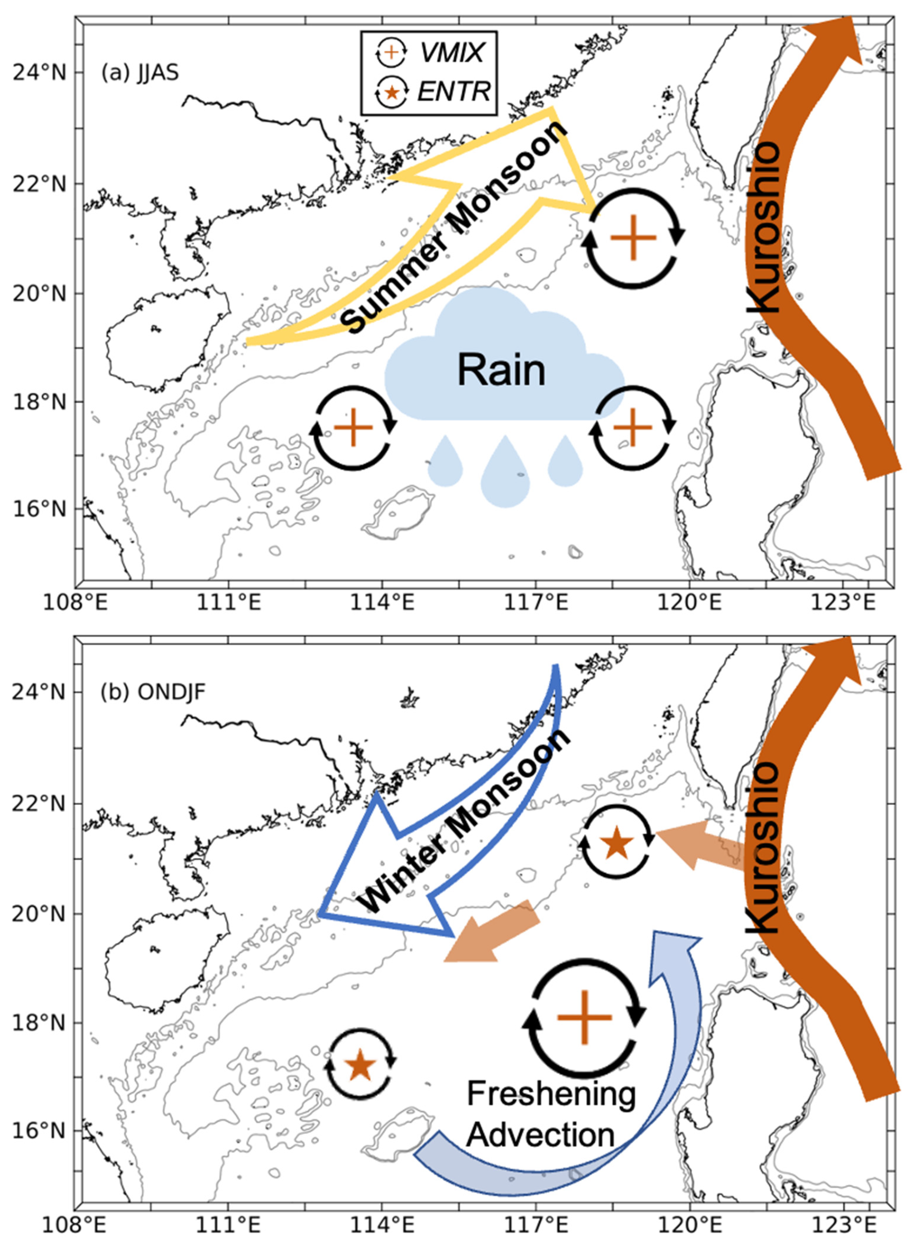
As summarized in Figure 10, during the summer monsoon the NSCS receives a large amount of freshwater from precipitation, which is the main cause of the basin-scale MLS reduction. The continuous atmospheric freshwater input forms a center of low salinity waters to the west of Luzon Island and enlarges the vertical salinity difference between that in the ML and just below it, and drives an increase in vertical mixing to balance the surface freshwater input. At the same time, the relatively fresher waters of WL can be advected northward by the seasonal circulation and cause a horizontal freshwater input in WLS. This together with the local atmospheric freshwater input is balanced by vertical processes that are also mainly associated with vertical mixing, but in mechanism are related to the internal wave-induced strong background turbulent mixing in the summer. During the winter monsoon, the intrusion and spreading of western Pacific water over the NSCS could modify the MLS structure and cause a larger entrainment than vertical mixing in regions such as WLS and EXS, where the effect of vertical mixing also decreases with the slackening of the seasonal internal wave activities. However, this is not the case for WL. Here, the greatly enhanced meridional advection by winter circulation brings in abundant fresher water from lower latitude regions, such that the vertical salinity difference enlarges and the vertical mixing can reach the seasonal maximum in the balance of the surface freshwater input.
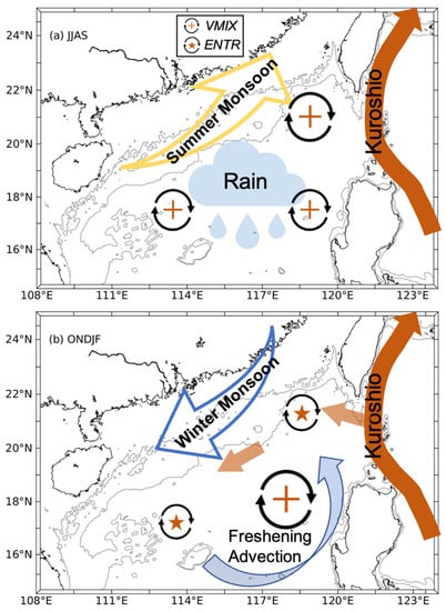
Figure 10.
Schematic plot showing the mechanism for the seasonal variation in MLS in the NSCS.
The analysis of the ML salinity budget reveals that vertical mixing, together with vertical entrainment, is vital to maintaining the seasonal variation in MLS in the NSCS. However, it is still difficult for us to verify the result carefully by quantitatively comparing each term in the budget between the model and observations. Perhaps in the future the robustness of our analysis can be assessed from more simulation results of the state-of-the-art ocean general circulation models that use different parameterizations of vertical physics, horizontal resolution, and/or forcing data sets.
Author Contributions
Y.C.: conceptualization, methodology, software, validation, formal analysis, writing—original draft, writing—review and editing, and visualization. C.X.: writing—review and editing. Y.Z.: writing—review and editing. Z.L.: writing—review and editing, supervision, and funding acquisition. All authors have read and agreed to the published version of the manuscript.
Funding
This research was funded by the Innovation Group Project of Southern Marine Science and Engineering Guangdong Laboratory (Zhuhai) (No. 311021006).
Institutional Review Board Statement
Not applicable.
Informed Consent Statement
Not applicable.
Data Availability Statement
Not applicable.
Acknowledgments
We thank the Asia–Pacific Data Research Center for its publicly accessible datasets.
Conflicts of Interest
The authors declare no conflict of interest.
References
- Liu, W.T.; Xie, X.S. Spacebased observations of the seasonal changes of South Asian monsoons and oceanic responses. Geophys. Res. Lett. 1999, 26, 1473–1476. [Google Scholar] [CrossRef]
- Chu, P.C.; Edmons, N.L.; Fan, C.W. Dynamical mechanisms for the South China Sea seasonal circulation and thermohaline variabilities. J. Phys. Oceanogr. 1999, 29, 2971–2989. [Google Scholar] [CrossRef]
- Jilan, S. Overview of the South China Sea circulation and its influence on the coastal physical oceanography outside the Pearl River Estuary. Cont. Shelf Res. 2004, 24, 1745–1760. [Google Scholar] [CrossRef]
- Grosse, J.; Bombar, D.; Hai, N.D.; Lam, N.N.; Voss, M. The Mekong River plume fuels nitrogen fixation and determines phytoplankton species distribution in the South China Sea during low- and high-discharge season. Limnol. Oceanogr. 2010, 55, 1668–1680. [Google Scholar] [CrossRef]
- Lu, W.F.; Yan, X.H.; Jiang, Y.W. Winter bloom and associated upwelling northwest of the Luzon Island: A coupled physical-biological modeling approach. J. Geophys. Res. Oceans 2015, 120, 533–546. [Google Scholar] [CrossRef]
- Xue, H.J.; Chai, F.; Pettigrew, N.; Xu, D.Y.; Shi, M.; Xu, J.P. Kuroshio intrusion and the circulation in the South China Sea. J. Geophys. Res. Oceans 2004, 109, C02017. [Google Scholar] [CrossRef]
- Zeng, L.L.; Timothy Liu, W.; Xue, H.J.; Xiu, P.; Wang, D.X. Freshening in the South China Sea during 2012 revealed by Aquarius and in situ data. J. Geophys. Res. Oceans 2014, 119, 8296–8314. [Google Scholar] [CrossRef]
- Yi, D.L.L.; Melnichenko, O.; Hacker, P.; Potemra, J. Remote Sensing of Sea Surface Salinity Variability in the South China Sea. J. Geophys. Res. Oceans 2020, 125, e2020JC016827. [Google Scholar] [CrossRef]
- Zeng, L.L.; Wang, D.X.; Xiu, P.; Shu, Y.Q.; Wang, Q.; Chen, J. Decadal variation and trends in subsurface salinity from 1960 to 2012 in the northern South China Sea. Geophys. Res. Lett. 2016, 43, 12181–12189. [Google Scholar] [CrossRef]
- Zeng, L.L.; Chassignet, E.P.; Xu, X.B.; Wang, D.X. Multi-decadal changes in the South China Sea mixed layer salinity. Clim Dynam 2021, 57, 435–449. [Google Scholar] [CrossRef]
- Zeng, L.L.; Wang, D.X. Seasonal variations in the barrier layer in the South China Sea: Characteristics, mechanisms and impact of warming. Clim. Dynam. 2017, 48, 1911–1930. [Google Scholar] [CrossRef]
- Yu, L.S. A global relationship between the ocean water cycle and near-surface salinity. J. Geophys. Res. Oceans 2011, 116, C10025. [Google Scholar] [CrossRef]
- Song, Y.T.; Lee, T.; Moon, J.H.; Qu, T.D.; Yueh, S. Modeling skin-layer salinity with an extended surface-salinity layer. J. Geophys. Res. Oceans 2015, 120, 1079–1095. [Google Scholar] [CrossRef]
- Köhler, J.; Serra, N.; Bryan, F.O.; Johnson, B.K.; Stammer, D. Mechanisms of Mixed-Layer Salinity Seasonal Variability in the Indian Ocean. J. Geophys. Res. Oceans 2018, 123, 466–496. [Google Scholar] [CrossRef]
- Gao, S.; Qu, T.D.; Nie, X.W. Mixed layer salinity budget in the tropical Pacific Ocean estimated by a global GCM. J. Geophys. Res. Oceans 2014, 119, 8255–8270. [Google Scholar] [CrossRef]
- Akhil, V.P.; Durand, F.; Lengaigne, M.; Vialard, J.; Keerthi, M.G.; Gopalakrishna, V.V.; Deltel, C.; Papa, F.; Montegut, C.D. A modeling study of the processes of surface salinity seasonal cycle in the Bay of Bengal. J. Geophys. Res. Oceans 2014, 119, 3926–3947. [Google Scholar] [CrossRef]
- Da-Allada, C.Y.; du Penhoat, Y.; Jouanno, J.; Alory, G.; Hounkonnou, N.M. Modeled mixed-layer salinity balance in the Gulf of Guinea: Seasonal and interannual variability. Ocean. Dyn. 2014, 64, 1783–1802. [Google Scholar] [CrossRef]
- Yan, Y.; Wang, G.; Wang, C.; Su, J. Low-salinity water off West Luzon Island in summer. J. Geophys. Res. Oceans 2015, 120, 3011–3021. [Google Scholar] [CrossRef]
- Shchepetkin, A.F.; McWilliams, J.C. The regional oceanic modeling system (ROMS): A split-explicit, free-surface, topography-following-coordinate oceanic model. Ocean. Model. 2005, 9, 347–404. [Google Scholar] [CrossRef]
- Shchepetkin, A.F.; McWilliams, J.C. Ocean forecasting in terrain-following coordinates: Formulation and skill assessment of the regional ocean modeling system (vol 227, pg 3595, 2008). J. Comput. Phys. 2009, 228, 8985–9000. [Google Scholar] [CrossRef]
- Gan, J.P.; Liu, Z.Q.; Liang, L.L. Numerical modeling of intrinsically and extrinsically forced seasonal circulation in the China Seas: A kinematic study. J. Geophys. Res. Oceans 2016, 121, 4697–4715. [Google Scholar] [CrossRef]
- Lu, W.F.; Oey, L.Y.; Liao, E.H.; Zhuang, W.; Yan, X.H.; Jiang, Y.W. Physical modulation to the biological productivity in the summer Vietnam upwelling system. Ocean Sci. 2018, 14, 1303–1320. [Google Scholar] [CrossRef]
- Large, W.G.; McWilliams, J.C.; Doney, S.C. Oceanic vertical mixing: A review and a model with a nonlocal boundary layer parameterization. Rev. Geophys. 1994, 32, 363–403. [Google Scholar] [CrossRef]
- Yu, L.S.; Weller, R.A. Objectively analyzed air-sea heat fluxes for the global ice-free oceans (1981–2005). Bull. Am. Meteorol. Soc. 2007, 88, 527–540. [Google Scholar] [CrossRef]
- Huffman, G.J.; Adler, R.F.; Bolvin, D.T.; Gu, G.J.; Nelkin, E.J.; Bowman, K.P.; Hong, Y.; Stocker, E.F.; Wolff, D.B. The TRMM multisatellite precipitation analysis (TMPA): Quasi-global, multiyear, combined-sensor precipitation estimates at fine scales. J. Hydrometeorol. 2007, 8, 38–55. [Google Scholar] [CrossRef]
- Bonjean, F.; Lagerloef, G.S.E. Diagnostic model and analysis of the surface currents in the tropical Pacific Ocean. J. Phys. Oceanogr. 2002, 32, 2938–2954. [Google Scholar] [CrossRef]
- Willmott, C.J. On the Validation of Models. Phys. Geogr. 1981, 2, 184–194. [Google Scholar] [CrossRef]
- Chu, P.C.; Chang, C.P. South china sea warm pool in boreal spring. Adv. Atmos. Sci. 1997, 14, 195–206. [Google Scholar] [CrossRef]
- Wang, D.X.; Liu, Q.Y.; Xie, Q.; He, Z.G.; Zhuang, W.; Shu, Y.Q.; Xiao, X.J.; Hong, B.; Wu, X.Y.; Sui, D.D. Progress of regional oceanography study associated with western boundary current in the South China Sea. Chin. Sci. Bull. 2013, 58, 1205–1215. [Google Scholar] [CrossRef]
- Qu, T.D. Upper-layer circulation in the South China Sea. J. Phys. Oceanogr. 2000, 30, 1450–1460. [Google Scholar] [CrossRef]
- Sommer, A.; Reverdin, G.; Kolodziejczyk, N.; Boutin, J. Sea Surface Salinity and Temperature Budgets in the North Atlantic Subtropical Gyre during SPURS Experiment: August 2012–August 2013. Front. Mar. Sci. 2015, 2, 107. [Google Scholar] [CrossRef]
- Ren, L.; Speer, K.; Chassignet, E.P. The mixed layer salinity budget and sea ice in the Southern Ocean. J. Geophys. Res. Oceans 2011, 116, C08031. [Google Scholar] [CrossRef]
- Li, R.; Stephen, C.R. Seasonal Salt Budget in the Northeast Pacific Ocean. J. Geophys. Res. Oceans 2008, 114, C12004. [Google Scholar]
- Mignot, J.; Frankignoul, C. Interannual to interdecadal variability of sea surface salinity in the Atlantic and its link to the atmosphere in a coupled model. J. Geophys. Res. Oceans 2004, 109, C04005. [Google Scholar] [CrossRef]
- Vinayachandran, P.N.; Nanjundiah, R.S. Indian Ocean sea surface salinity variations in a coupled model. Clim. Dynam. 2009, 33, 245–263. [Google Scholar] [CrossRef]


Disclaimer/Publisher’s Note: The statements, opinions and data contained in all publications are solely those of the individual author(s) and contributor(s) and not of MDPI and/or the editor(s). MDPI and/or the editor(s) disclaim responsibility for any injury to people or property resulting from any ideas, methods, instructions or products referred to in the content. |
© 2023 by the authors. Licensee MDPI, Basel, Switzerland. This article is an open access article distributed under the terms and conditions of the Creative Commons Attribution (CC BY) license (https://creativecommons.org/licenses/by/4.0/).