

Research on the Transport of Typical Pollutants in the Yellow Sea with Flow and Wind Fields

Abstract
:1. Introduction
2. Model and Methodology
2.1. Model Description
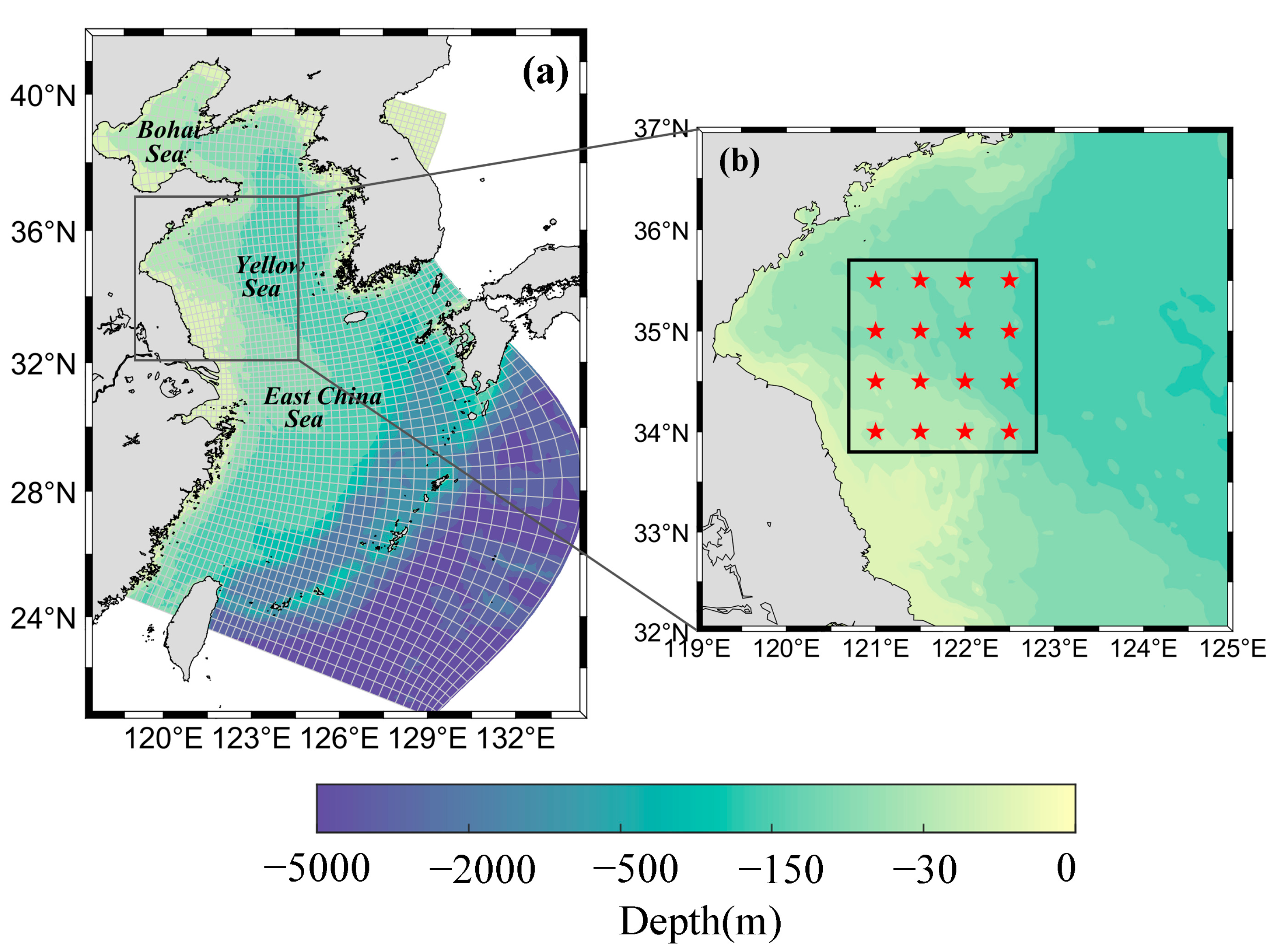
2.2. Hydrodynamic Background Field
2.3. Experimental Design
3. Results
3.1. Variability of Environmental Factors
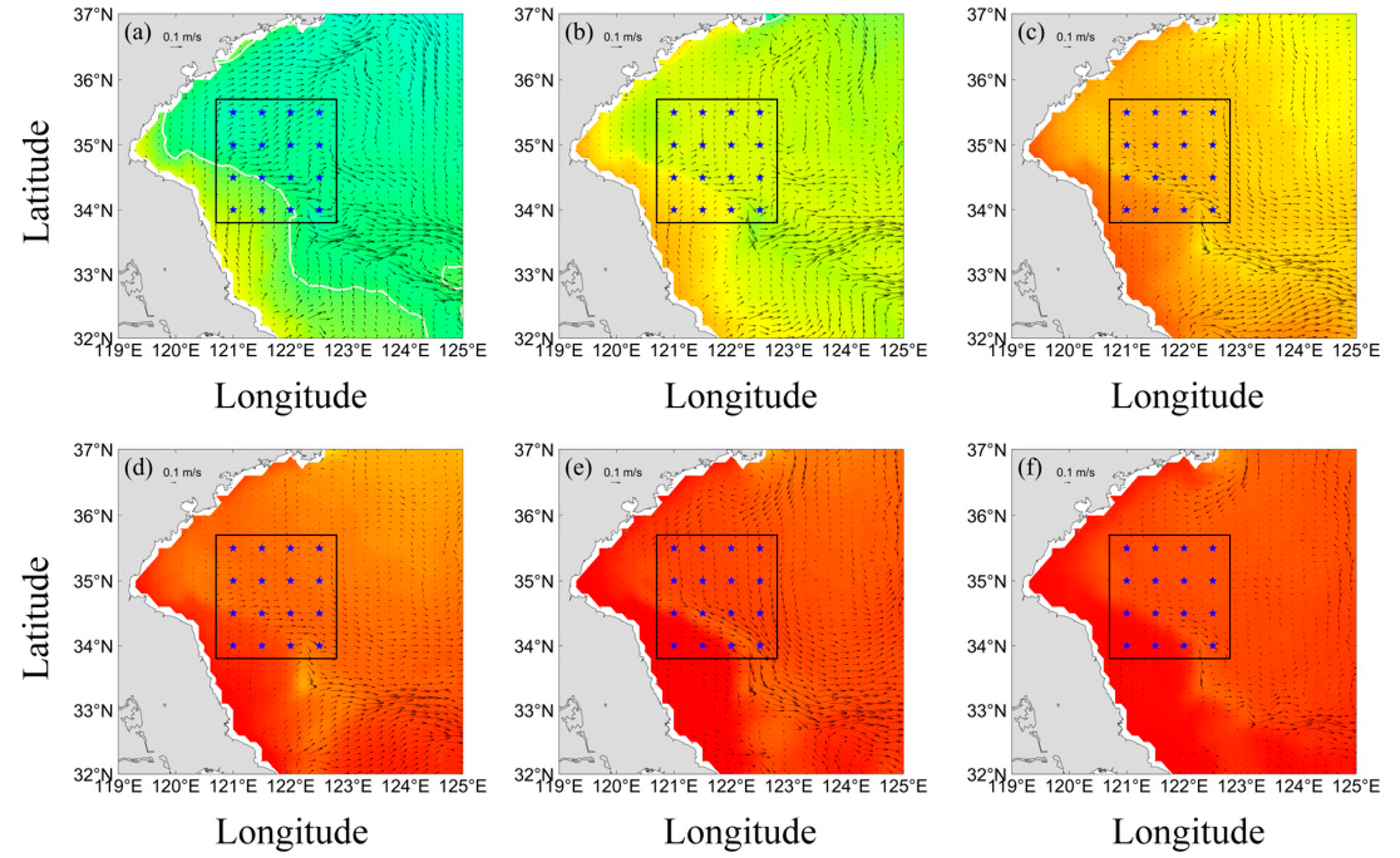
3.1.1. Current
3.1.2. Temperature
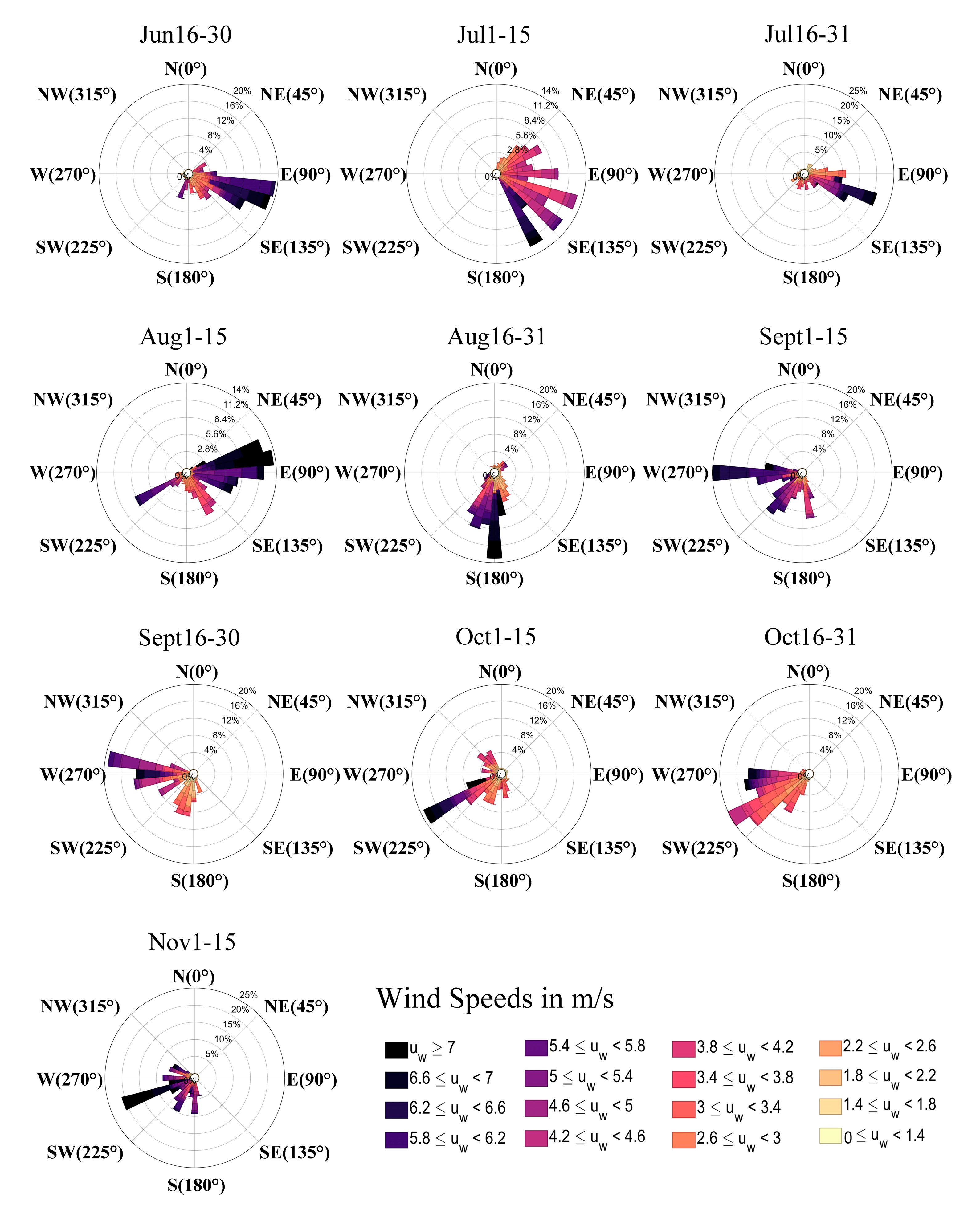
3.1.3. Wind
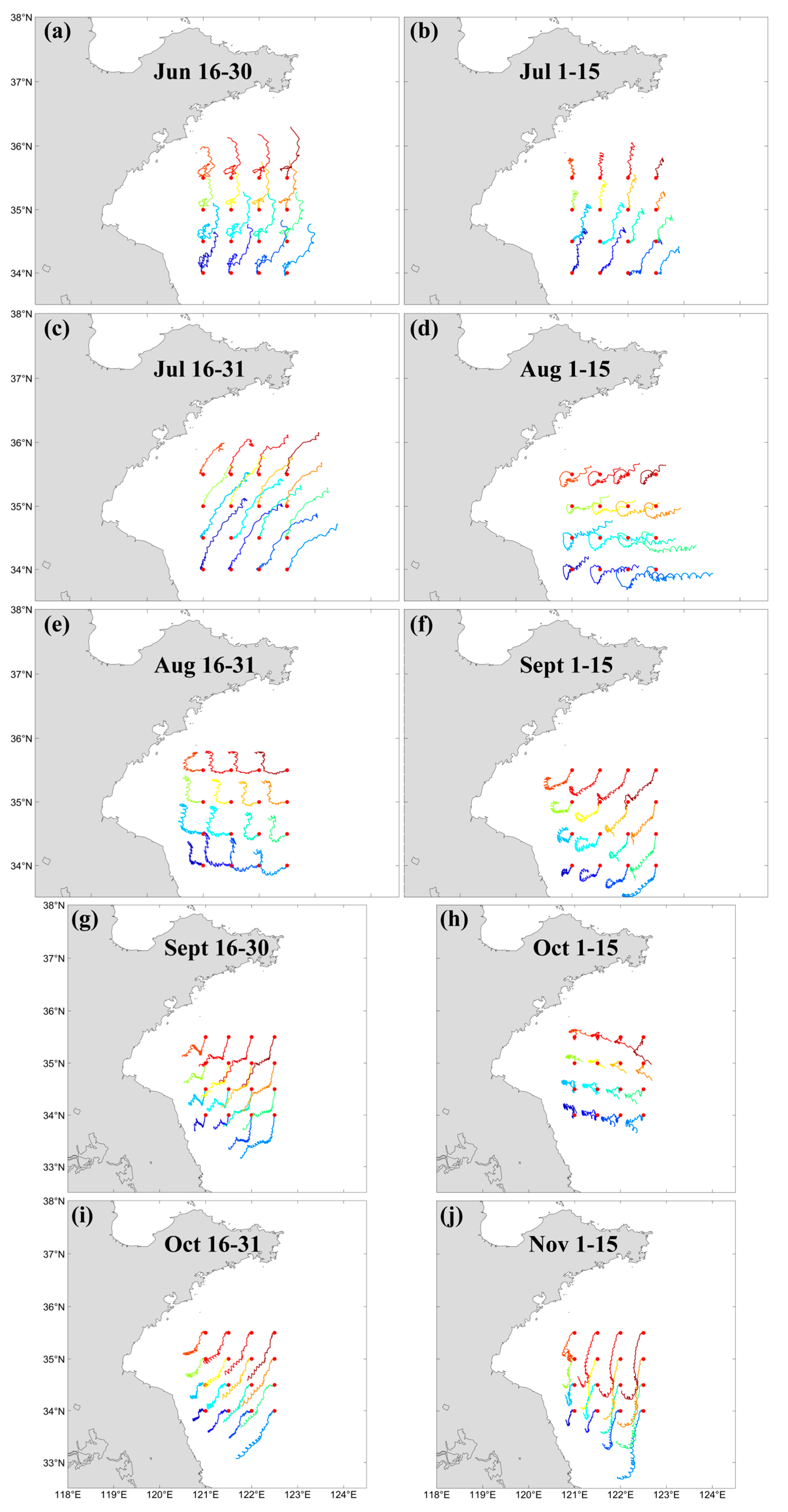
3.2. Model Results
3.3. Empirical Relationship
3.3.1. Quantitative Analysis
3.3.2. Derivation of Formulas
3.4. Design of Aquaculture Vessel Navigation Routes
3.5. Prospects on Model Development
4. Summary and Conclusions
Supplementary Materials
Author Contributions
Funding
Institutional Review Board Statement
Informed Consent Statement
Data Availability Statement
Acknowledgments
Conflicts of Interest
References
- Cabello, F.C.; Godfrey, H.P.; Tomova, A.; Ivanova, L.; Doelz, H.; Millanao, A.; Buschmann, A.H. Antimicrobial Use in Aquaculture Re-Examined: Its Relevance to antimicrobial Resistance and to Animal and Human Health. Environ. Microbiol. 2013, 15, 1917–1942. [Google Scholar] [CrossRef] [PubMed]
- Liu, X.; Lu, S.; Guo, W.; Xi, B.; Wang, W. Antibiotics in the Aquatic Environments: A Review of Lakes, China. Sci. Total Environ. 2018, 627, 1195–1208. [Google Scholar] [CrossRef]
- Xu, J.; Han, L.; Yin, W. Research on the Ecologicalization Efficiency of Mariculture Industry in China and Its Influencing Factors. Mar. Policy 2022, 137, 104935. [Google Scholar] [CrossRef]
- Schrenk, D.; Bignami, M.; Bodin, L.; Chipman, J.K.; del Mazo, J.; Grasl-Kraupp, B.; Hogstrand, C.; Hoogenboom, L.; Leblanc, J.-C.; Nebbia, C.S.; et al. Risk to Human Health Related to the Presence of Perfluoroalkyl in Food. EFSA J. 2020, 18, e06223. [Google Scholar] [CrossRef] [PubMed]
- Winiarski, L.D.; Frick, W.F. Cooling Tower Plume Model; US Environmental Protection Agency, Office of Research and Development: Washington, DC, USA, 1976. [Google Scholar]
- Fannelop, T.; Sjoen, K. Hydrodynamics of Underwater Blowouts. In Proceedings of the 18th Aerospace Sciences Meeting, Pasadena, CA, USA, 14–16 January 1980; p. 219. [Google Scholar]
- Johansen, Ø. The Halten Bank Experiment-Observations and Model Studies of Drift and Fate of Oil in the Marine Environment. In Proceedings of the 11th Arctic Marine Oil Spill Program (AMOP) Techn. Seminar. Environment Canada, Ottawa, ON, Canada, June 1984; pp. 18–36. [Google Scholar]
- Elliott, A.J. Shear Diffusion and the Spread of Oil in the Surface Layers of the North Sea. Dtsch. Hydrogr. Z. 1986, 39, 113–137. [Google Scholar] [CrossRef]
- Rye, H. Model for Calculation of Underwater Blow-out Plume. In Proceedings of the Arctic and Marine Oilspill Program Technical Seminar; Ministry of Supply and Services, Edmonton, AB, Canada, 8–10 June 1994; p. 849. [Google Scholar]
- Zheng, L.; Yapa, P.D. Simulation of Oil Spills from Underwater Accidents II: Model Verification. J. Hydraul. Res. 1998, 36, 117–134. [Google Scholar] [CrossRef]
- Lonin, S.A. Lagrangian Model for Oil Spill Diffusion at Sea. Spill Sci. Technol. Bull. 1999, 5, 331–336. [Google Scholar] [CrossRef]
- Johansen, Ø. DeepBlow–a Lagrangian Plume Model for Deep Water Blowouts. Spill Sci. Technol. Bull. 2000, 6, 103–111. [Google Scholar] [CrossRef]
- Zheng, L.; Yapa, P.D. Modeling Gas Dissolution in Deepwater Oil/Gas Spills. J. Mar. Syst. 2002, 31, 299–309. [Google Scholar] [CrossRef]
- Lee, J.H.; Pang, I.; Moon, I.; Ryu, J. On Physical Factors That Controlled the Massive Green Tide Occurrence along the Southern Coast of the Shandong Peninsula in 2008: A Numerical Study Using a Particle-tracking Experiment. J. Geophys. Res. Ocean. 2011, 116, C12036. [Google Scholar] [CrossRef]
- Putman, N.F.; Goni, G.J.; Gramer, L.J.; Hu, C.; Johns, E.M.; Trinanes, J.; Wang, M. Simulating Transport Pathways of Pelagic Sargassum from the Equatorial Atlantic into the Caribbean Sea. Prog. Oceanogr. 2018, 165, 205–214. [Google Scholar] [CrossRef]
- Wang, M.; Hu, C. Mapping and Quantifying Sargassum Distribution and Coverage in the Central West Atlantic Using MODIS Observations. Remote Sens. Environ. 2016, 183, 350–367. [Google Scholar] [CrossRef]
- Keesing, J.K.; Liu, D.; Fearns, P.; Garcia, R. Inter-and Intra-Annual Patterns of Ulva Prolifera Green Tides in the Yellow Sea during 2007–2009, Their Origin and Relationship to the Expansion of Coastal Seaweed Aquaculture in China. Mar. Pollut. Bull. 2011, 62, 1169–1182. [Google Scholar] [CrossRef]
- Jalón-Rojas, I.; Wang, X.H.; Fredj, E. A 3D Numerical Model to Track Marine Plastic Debris (TrackMPD): Sensitivity of Microplastic Trajectories and Fates to Particle Dynamical Properties and Physical Processes. Mar. Pollut. Bull. 2019, 141, 256–272. [Google Scholar] [CrossRef] [PubMed]
- Alosairi, Y.; Alsulaiman, N. Hydro-Environmental Processes Governing the Formation of Hypoxic Parcels in an Inverse Estuarine Water Body: Model Validation and Discussion. Mar. Pollut. Bull. 2019, 144, 92–104. [Google Scholar] [CrossRef] [PubMed]
- Van Utenhove, E. Modelling the Transport and Fate of Buoyant Macroplastics in Coastal Waters. Master's Thesis, Delft University of Technology, Delft, The Netherland, December 2019. [Google Scholar]
- Aiyer, A.K.; Yang, D.; Chamecki, M.; Meneveau, C. A Population Balance Model for Large Eddy Simulation of Polydisperse Droplet Evolution. J. Fluid. Mech. 2019, 878, 700–739. [Google Scholar] [CrossRef]
- Cao, R.; Chen, H.; Li, H.; Fu, H.; Wang, Y.; Bao, M.; Tuo, W.; Lv, X. A Mesoscale Assessment of Sinking Oil during Dispersant Treatment. Ocean. Eng. 2022, 263, 112341. [Google Scholar] [CrossRef]
- Cui, F.; Boufadel, M.C.; Geng, X.; Gao, F.; Zhao, L.; King, T.; Lee, K. Oil Droplets Transport under a Deep-water Plunging Breaker: Impact of Droplet Inertia. J. Geophys. Res. Ocean. 2018, 123, 9082–9100. [Google Scholar] [CrossRef]
- Stolzenbach, K.D.; Madsen, O.S.; Adams, E.E.; Pollack, A.M.; Cooper, C. A Review and Evaluation of Basic Techniques for Predicting the Behavior of Surface Oil Slicks; Report (Massachusetts Institute of Technology. Sea Grant Program), no. MITSG 77-8; Massachusetts Institute of Technology: Cambridge, MA, USA, 1977. [Google Scholar]
- Wang, S.D.; Shen, Y.M.; Zheng, Y.H. Two-Dimensional Numerical Simulation for Transport and Fate of Oil Spills in Seas. Ocean. Eng. 2005, 32, 1556–1571. [Google Scholar] [CrossRef]
- Li, Y.; Chen, H.; Lv, X. Impact of Error in Ocean Dynamical Background, on the Transport of Underwater Spilled Oil. Ocean. Model 2018, 132, 30–45. [Google Scholar] [CrossRef]
- Samuels, W.B.; Huang, N.E.; Amstutz, D.E. An Oilspill Trajectory Analysis Model with a Variable Wind Deflection Angle. Ocean. Eng. 1982, 9, 347–360. [Google Scholar] [CrossRef]
- Wang, J.; Shen, Y. Modeling Oil Spills Transportation in Seas Based on Unstructured Grid, Finite-Volume, Wave-Ocean Model. Ocean. Model 2010, 35, 332–344. [Google Scholar] [CrossRef]
- Pan, Q.; Yu, H.; Daling, P.S.; Zhang, Y.; Reed, M.; Wang, Z.; Li, Y.; Wang, X.; Wu, L.; Zhang, Z. Fate and Behavior of Sanchi Oil Spill Transported by the Kuroshio during January–February 2018. Mar. Pollut. Bull. 2020, 152, 110917. [Google Scholar] [CrossRef]
- Boufadel, M.; Liu, R.; Zhao, L.; Lu, Y.; Özgökmen, T.; Nedwed, T.; Lee, K. Transport of Oil Droplets in the Upper Ocean: Impact of the Eddy Diffusivity. J. Geophys. Res. Oceans 2020, 125, e2019JC015727. [Google Scholar] [CrossRef]
- Bandara, U.C.; Yapa, P.D. Bubble Sizes, Breakup, and Coalescence in Deepwater Gas/Oil Plumes. J. Hydraul. Eng. 2011, 137, 729–738. [Google Scholar] [CrossRef]
- Khater, E.-S.G.; Bahnasawy, A.H.; Ali, S.A. Physical and Mechanical Properties of Fish Feed Pellets. J. Food Process Technol. 2014, 5, 1. [Google Scholar]
- Haidvogel, D.B.; Blanton, J.; Kindle, J.C.; Lynch, D.R. Coastal Ocean Modeling: Processes and Real-Time Systems. Oceanography 2000, 13, 35–46. [Google Scholar] [CrossRef]
- Shchepetkin, A.F.; McWilliams, J.C. The Regional Oceanic Modeling System (ROMS): A Split-Explicit, Free-Surface, Topography-Following-Coordinate Oceanic Model. Ocean. Model 2005, 9, 347–404. [Google Scholar] [CrossRef]
- Li, M.; Rong, Z. Effects of Tides on Freshwater and Volume Transports in the Changjiang River Plume. J. Geophys. Res. Ocean. 2012, 117. [Google Scholar] [CrossRef]
- Cao, R.; Chen, H.; Rong, Z.; Lv, X. Impact of Ocean Waves on Transport of Underwater Spilled Oil in the Bohai Sea. Mar. Pollut. Bull. 2021, 171, 112702. [Google Scholar] [CrossRef]
- Rong, Z.; Li, M. Tidal Effects on the Bulge Region of Changjiang River Plume. Estuar. Coast. Shelf Sci. 2012, 97, 149–160. [Google Scholar] [CrossRef]
- Egbert, G.D.; Bennett, A.F.; Foreman, M.G.G. TOPEX/POSEIDON Tides Estimated Using a Global Inverse Model. J. Geophys. Res. Ocean. 1994, 99, 24821–24852. [Google Scholar] [CrossRef]
- Egbert, G.D.; Erofeeva, S.Y. Efficient Inverse Modeling of Barotropic Ocean Tides. J. Atmos. Ocean. Technol. 2002, 19, 183–204. [Google Scholar] [CrossRef]
- Chapman, D.C. Numerical Treatment of Cross-Shelf Open Boundaries in a Barotropic Coastal Ocean Model. J. Phys. Oceanogr. 1985, 15, 1060–1075. [Google Scholar] [CrossRef]
- Flather, R.A. A Tidal Model of the Northwest European Continental Shelf. Mem. Soc. Roy. Sci. Liege 1976, 10, 141–164. [Google Scholar]
- Orlanski, I. A Simple Boundary Condition for Unbounded Hyperbolic Flows. J. Comput. Phys. 1976, 21, 251–269. [Google Scholar] [CrossRef]
- Chen, Y.; Huang, W.; Shan, X.; Chen, J.; Weng, H.; Yang, T.; Wang, H. Growth Characteristics of Cage-Cultured Large Yellow Croaker Larimichthys Crocea. Aquac. Rep. 2020, 16, 100242. [Google Scholar] [CrossRef]


| Model Parameters | Value |
|---|---|
| Release depth | 0 m |
| Release duration | 15 days |
| Simulation duration | 15 days |
| Particle quantity | 10,000 |
| Particle density | 500 kg/m3 |
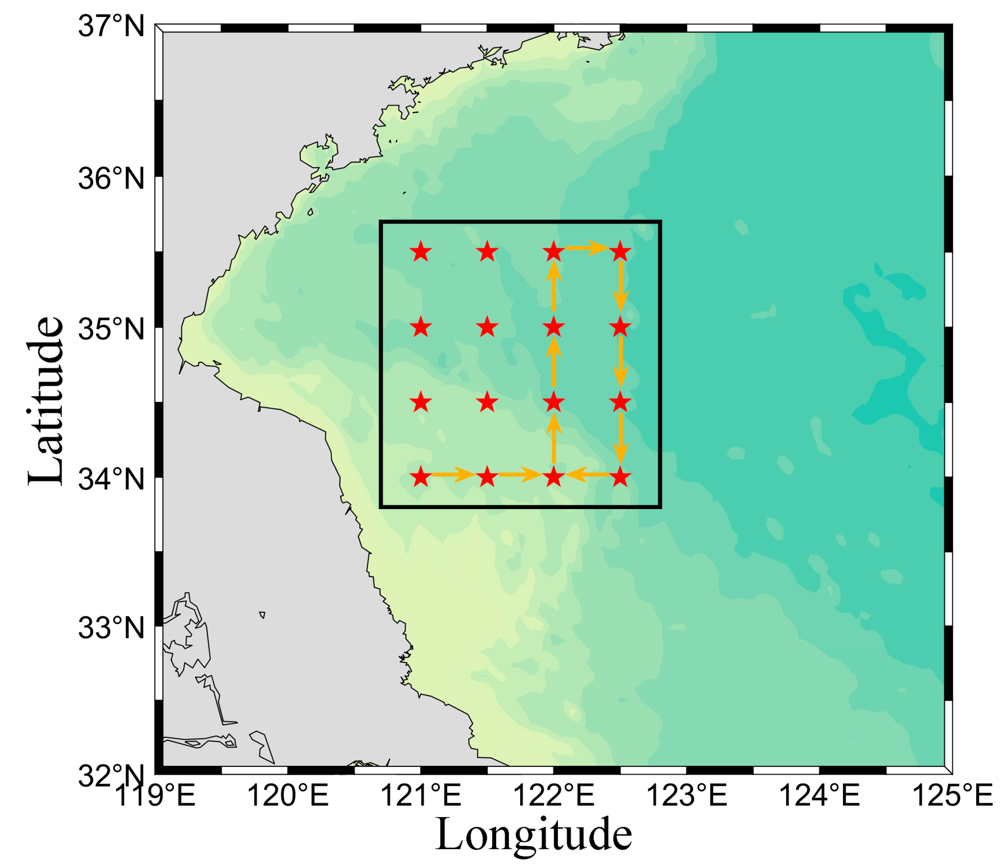
| Position | Lon. (°E) | Lat. (°N) | Position | Lon. (°E) | Lat. (°N) |
|---|---|---|---|---|---|
| 1 | 121 | 34 | 9 | 121 | 35 |
| 2 | 121.5 | 34 | 10 | 121.5 | 35 |
| 3 | 122 | 34 | 11 | 122 | 35 |
| 4 | 122.5 | 34 | 12 | 122.5 | 35 |
| 5 | 121 | 34.5 | 13 | 121 | 35.5 |
| 6 | 121.5 | 34.5 | 14 | 121.5 | 35.5 |
| 7 | 122 | 34.5 | 15 | 122 | 35.5 |
| 8 | 122.5 | 34.5 | 16 | 122.5 | 35.5 |
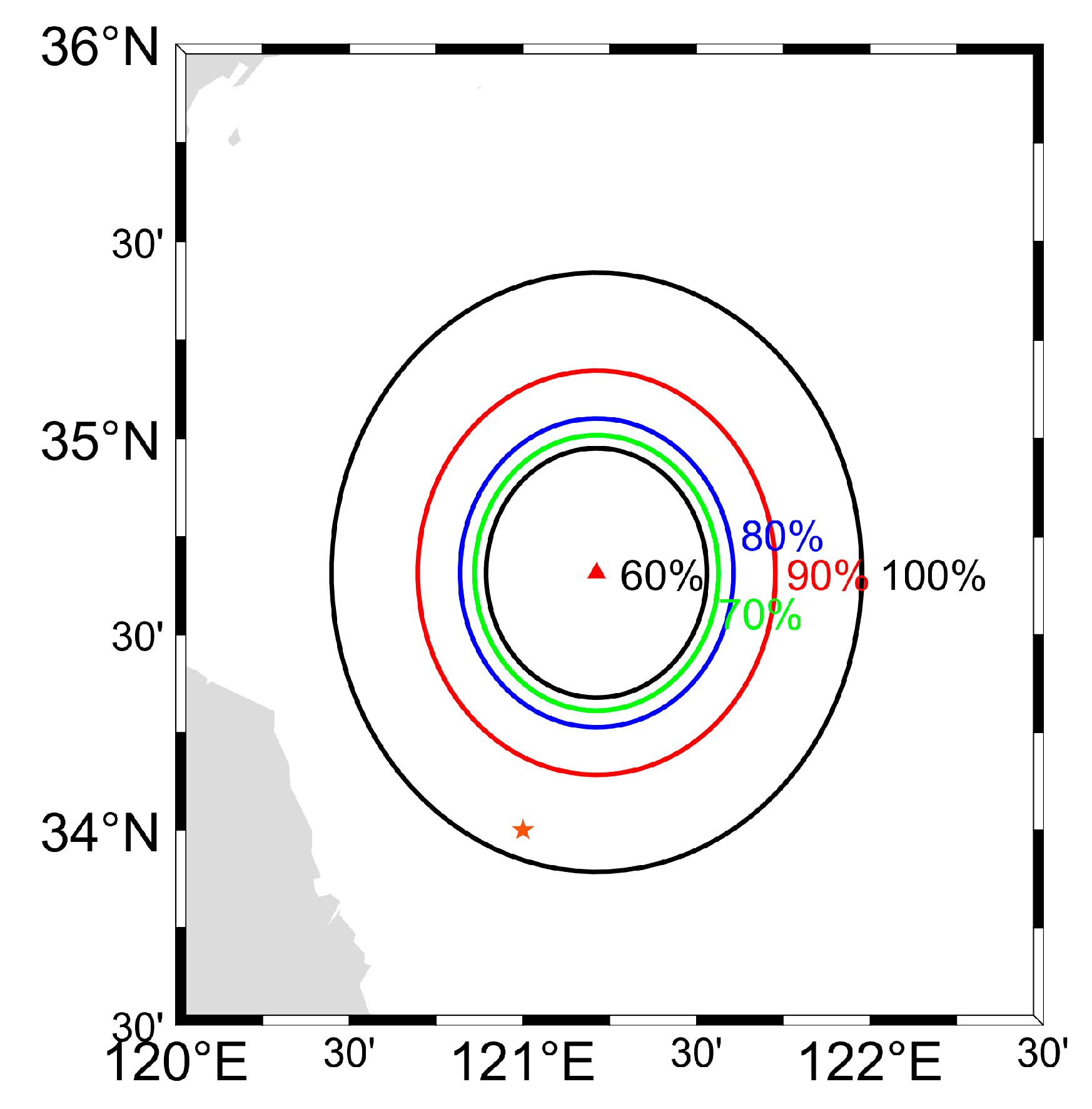
| Percentage | 100% | 90% | 80% | 70% | 60% |
|---|---|---|---|---|---|
| Radius R (km) | 84.98 | 57.33 | 43.81 | 39.10 | 35.40 |
| Average flow velocity (m/s) | 0.026 | 0.029 | 0.033 | 0.033 | 0.036 |
| Average flow direction (°) | 94.40 | 87.89 | 83.99 | 83.76 | 81.73 |
| Percentage | 100% | 90% | 80% | 70% | 60% |
|---|---|---|---|---|---|
| Direction 1 (°) | 75.01 | 75.01 | 75.01 | 75.01 | 75.01 |
| Direction 2 (°) | 94.40 | 87.89 | 83.99 | 83.76 | 81.73 |
| Angle difference θ | 19.39 | 12.88 | 8.98 | 8.75 | 6.72 |
| Percentage | 100% | 90% | 80% | 70% | 60% |
|---|---|---|---|---|---|
| Distance 1 (km) | 75.60 | 75.60 | 75.60 | 75.60 | 75.60 |
| Distance 2 (km) | 139.21 | 142.33 | 148.07 | 148.54 | 151.92 |
| Distance Ratio β | 1.84 | 1.88 | 1.96 | 1.96 | 2.01 |
Disclaimer/Publisher’s Note: The statements, opinions and data contained in all publications are solely those of the individual author(s) and contributor(s) and not of MDPI and/or the editor(s). MDPI and/or the editor(s) disclaim responsibility for any injury to people or property resulting from any ideas, methods, instructions or products referred to in the content. |
© 2023 by the authors. Licensee MDPI, Basel, Switzerland. This article is an open access article distributed under the terms and conditions of the Creative Commons Attribution (CC BY) license (https://creativecommons.org/licenses/by/4.0/).
Share and Cite
Wang, N.; Cao, R.; Lv, X.; Shi, H. Research on the Transport of Typical Pollutants in the Yellow Sea with Flow and Wind Fields. J. Mar. Sci. Eng. 2023, 11, 1710. https://doi.org/10.3390/jmse11091710
Wang N, Cao R, Lv X, Shi H. Research on the Transport of Typical Pollutants in the Yellow Sea with Flow and Wind Fields. Journal of Marine Science and Engineering. 2023; 11(9):1710. https://doi.org/10.3390/jmse11091710
Chicago/Turabian StyleWang, Nan, Ruichen Cao, Xianqing Lv, and Honghua Shi. 2023. "Research on the Transport of Typical Pollutants in the Yellow Sea with Flow and Wind Fields" Journal of Marine Science and Engineering 11, no. 9: 1710. https://doi.org/10.3390/jmse11091710