A Review of Application of Machine Learning in Storm Surge Problems

Abstract

The rise of machine learning (ML) has significantly advanced the field of coastal oceanography. This review aims to examine the existing deficiencies in numerical predictions of storm surges and the effort that has been made to improve the predictive accuracy through the application of ML. The readers are guided through the steps required to implement ML algorithms, from the first step of formulating problems to data collection and determination of input features to model selection, development and evaluation. Additionally, the review explores the application of hybrid methods, which combine the bilateral advantages of data-driven methods and physics-based models. Furthermore, the strengths and limitations of ML methods in predicting storm surges are thoroughly discussed, and research gaps are identified. Finally, we outline a vision toward a trustworthy and reliable storm surge forecasting system by introducing novel physics-informed ML techniques. We are meant to provide a primer for beginners and experts in coastal ocean sciences who share a keen interest in ML methodologies in the context of storm surge problems.

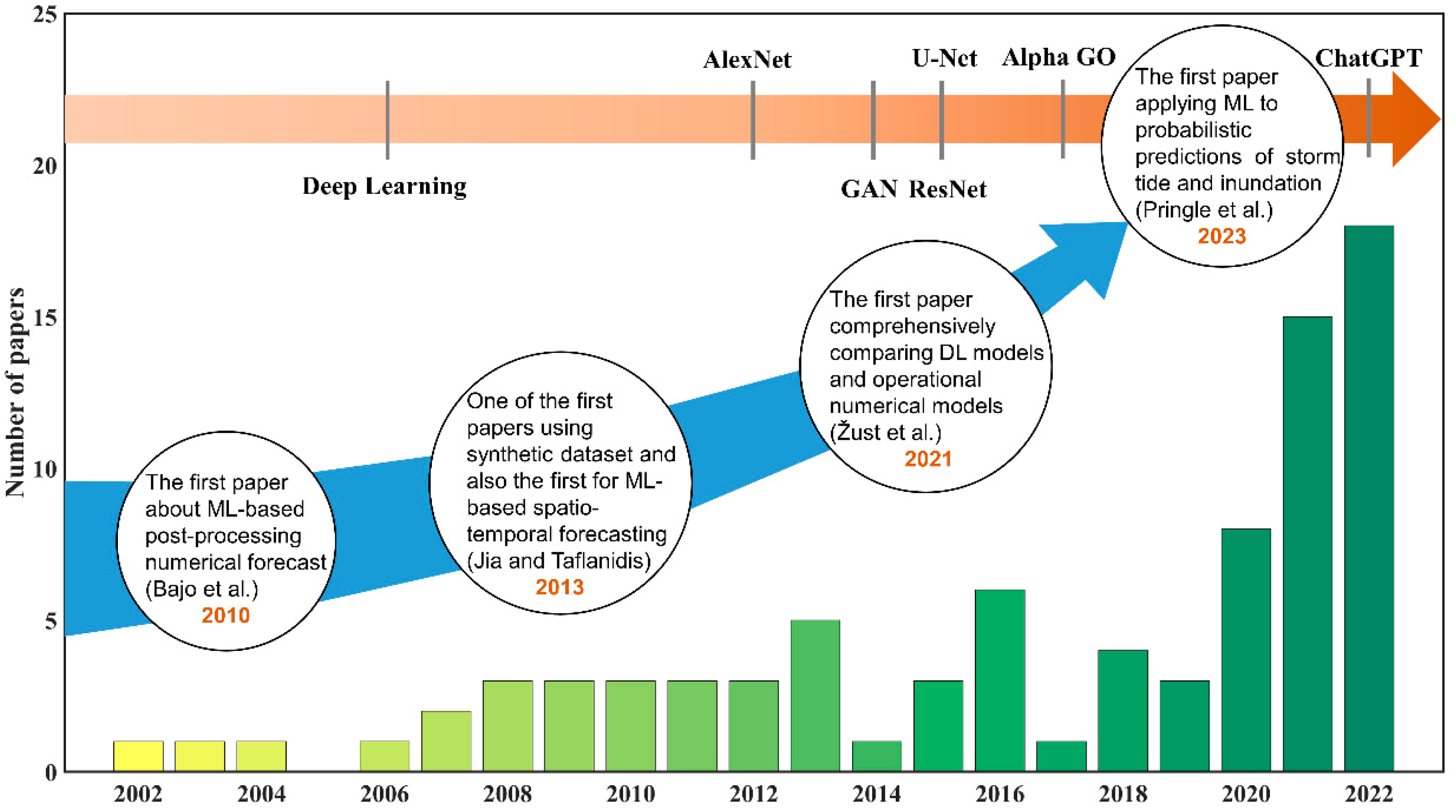
1. Introduction

Storm surge refers to the abnormal rise in sea level associated with low-pressure weather systems and is amplified in the coastal regions where intricate air–land–ocean interactions play a key role. This review mainly focuses on storm surges induced by tropical cyclones (TCs), which are the most deadly and impactful global disasters, especially for coastal communities [1], while also covering storm surges triggered by other atmospheric forcings. Many historical events of devastating misfortunes have been documented. For instance, March 1999 witnessed the world record for a storm surge of 13 m height, which was caused by the landfall of TC Mahina in northeast Australia [2]. In 2005, catastrophic hurricane Katrina gave rise to a 4–7 m storm surge and at least 1833 fatalities and direct economic losses of $108 billion [3]. It’s shown that storm surges will likely become more severe in the near future decades under the projected climate changes [4], and therefore, much more attention should be paid to storm surges to boost the observations, theoretical discovery, and simulation and forecasting methods to reduce the losses of lives and the property damage.

The earliest recorded events of storm surges resulting from super typhoons can be traced back to the prehistoric period [5]. However, before the modern era, detailed, continuous and systematic monitoring of storm surges was not available. Present measurements of storm surges are through tidal gauges to monitor alongshore variations, satellite altimetry to capture cross-shelf features of storm surges (for the first time [6]), and the recently launched next-generation radar altimeter Surface Water and Ocean Topography (SWOT) will also help forecast and characterize 2D storm surge features at a spatial resolution of 50 m [7]. However, the difficulty of data availability, the insufficiency in quantity, and the weakness in quality of storm surges still impede the rapid development of ML models, calling for comprehensive synthetic datasets to be built by numerical models.

The theory of geophysical fluid dynamics (GFD) takes its rise from the ancient Greek sage Archimedes, who discovered the physical law of buoyancy. However, the era of modern GFD has its roots in the linearization of Navier–Stokes (NS) equations [8], which enhanced the understanding of meteorology and oceanography. The 2D shallow-water equations [9] derived from the NS equations are the basic equations where the storm surge models of vertically mixed coastal waters have been developed:

$$\frac{\partial u}{\partial \mathrm{t}}+u\frac{\partial u}{\partial x}+v\frac{\partial u}{\partial y}-fv=-\frac{1}{{\rho }_0}\frac{\partial p_{\mathrm{a}}}{\partial x}-g\frac{\partial \zeta }{\partial x}+\frac{\partial }{\partial x}\left(N_{\mathrm{h}}\frac{\partial u}{\partial x}\right)+\frac{\partial }{\partial y}\left(N_{\mathrm{h}}\frac{\partial u}{\partial y}\right)+\frac{{\tau }_{\mathrm{s}x}-{\tau }_{\mathrm{b}x}}{{\rho }_0\left(H+\zeta \right)}$$

(1)

$$\frac{\partial v}{\partial \mathrm{t}}+u\frac{\partial v}{\partial x}+v\frac{\partial v}{\partial y}+fu=-\frac{1}{{\rho }_0}\frac{\partial p_{\mathrm{a}}}{\partial y}-g\frac{\partial \zeta }{\partial y}+\frac{\partial }{\partial x}\left(N_{\mathrm{h}}\frac{\partial v}{\partial x}\right)+\frac{\partial }{\partial y}\left(N_{\mathrm{h}}\frac{\partial v}{\partial y}\right)+\frac{{\tau }_{\mathrm{s}y}-{\tau }_{\mathrm{b}y}}{{\rho }_0\left(H+\zeta \right)}$$

(2)

$$\frac{\partial \zeta }{\partial \mathrm{t}}+\frac{\partial u\left(H+\zeta \right)}{\partial x}+\frac{\partial v\left(H+\zeta \right)}{\partial y}=0$$

(3)

where $H$ is the mean water depth, $\zeta$ is water surface elevation from the mean, $f$ is the Coriolis parameter, $p_a$ is the atmospheric pressure, ${\rho }_0$ is the water density, $N_h$ is the horizontal eddy viscosity coefficient, $(u,v)$ is the vertically-averaged current velocity, $({\tau }_{sx},{\tau }_{sy})$ and $({\tau }_{bx},{\tau }_{by})$ are the surface wind stress and bottom friction stress, respectively. When numerically solving the storm surge equations, the water elevation $\zeta$ at the next time step can be expressed as a function of $\zeta$, and $u$, $v$ at the current time [10]. Similarly, the vertically-averaged current velocity $u$ and $v$ can be represented as a function of $p_a$, $N_h$, ${\tau }_s$ and ${\tau }_b$. The $\zeta$ at the next time step can be written as:

$${\zeta }^{t+1}=\mathcal{F}\left({\zeta }^t,u^t,v^t\right)=\mathcal{F}\left({\zeta }^t,p_a^t,N_h^t,{\tau }_s^t,{\tau }_b^t\right)$$

(4)

where $\mathcal{F}$ is the mapping function which remains unknown and can be learned by ML algorithms. The characteristics of the storm surge encompass at least six processes: direct wind effect, inverted barometer effect, Coriolis effect, waves, rainfall [11], tidal effects and so on. The nonlinear tide-surge interactions have been widely studied and proved to significantly influence the accurate predictions of storm surge [12,13].

With the basic understanding of storm surge, it’s of overarching concern for mankind to predict this disastrous ocean phenomenon prior to storm landfall. The emergence of numerical computing in the late 1940s enabled numerical modeling and forecasting storm surges to become practical. Numerical methods are now the most extensively used approach for storm surge predictions, such as the SLOSH (Sea, Lake and Overland Surges from Hurricane) [14], FVCOM (Finite-Volume Coastal Ocean Model) [15,16], and ADCIRC (ADvanced CIRCulation) model [17]. High-fidelity coupled dynamical models can provide accurate measures of storm surge and inundation depth [18,19], but they are too computationally expensive to be employed in real-time forecasting systems. In addition to some intrinsic uncertainties of numerical models, such as simplification of governing equations and initial/boundary conditions [20], the primary sources of operational forecast errors result from the abrupt variation of TC in track and intensity caused by the parametric TC wind field [21]. The average 24-h intensity official forecast errors of TCs over the North Atlantic, east Pacific, and western North Pacific are almost 10 kt [22], and the annual-mean position errors of TC track forecasts at RSMC-Tokyo, CMA and JTWC are near 100 km [23]. In addition, it’s difficult to greatly improve the forecast accuracy of TC tracks and intensity in numerical TC forecast models within a short period. Therefore, ensemble storm surge predictions considering varied typhoons have garnered much more traction and appeared in operational centers in recent years [24]. Undoubtedly, executing multiple runs for ensemble and probabilistic forecasting of storm surges requires more computational resources than deterministic forecasting. The efficiency-accuracy tradeoff encountered in storm-surge numerical forecasting is expected to be addressed by promising ML techniques.

Machine Learning is a sub-domain of artificial intelligence (AI) that renders computers the ability to perform selected tasks by ‘learning’ from data [8]. The unprecedented confluence of powerful computers, sophisticated algorithms, and big ocean data with the five-V (volume, variety, value, velocity and veracity) characteristics enables the ML to make inroads in the oceanography [25,26]. Many reviews have been provided to introduce beginners and experts in fluid dynamics, marine science and engineering and earth system modeling to AI methodologies [8,25,26,27,28,29,30,31,32,33,34,35]. In the last five years, the number of studies investigating the feasibility of ML methodologies in storm surge problems has been increasing, as depicted in Figure 1. Nevertheless, there remains no comprehensive review that summarizes current progress and issues and proposes future outlooks for researchers enthusiastic about this topic. For this reason, this paper is geared toward not only offering a well-directed review of ML tools in solving storm surge problems but also bringing some insight into the barriers and suggesting possible solutions.

The remainder of this paper follows the general workflow of developing an ML model targeted to a specific storm surge problem, as illustrated in Figure 2. Section 2 introduces different forms of formulating storm surge and coastal inundation prediction problems. Section 3 explains the data used for ML model training and some considerations required to make a good feature representation. In Section 4, the basic concepts of ML are presented, along with a summary of frequently used algorithms and error metrics for model evaluation. Section 5 reviews the application of hybrid methods in storm surge forecasting, showing great potential. Some common challenges and opportunities are discussed in Section 6 and Section 7, provide an introduction to physics-informed ML and a summary, and envision an improved storm surge warning system.

2. The Formulation of Prediction Problems

The initial step in constructing an ML model for predicting storm surge is formulating the problem, which involves defining a clear strategy to achieve your objective. In storm surge studies, previous studies primarily focused on several key aspects: the temporal evolution and peak values of water levels, the extent of onshore flooding, and the mapping of coastal inundation areas. Water level forecasting encompasses both storm surge and storm tide forecasting, with the latter aiming to predict water levels resulting from the combination of storm surge and the astronomical tide. Inundation refers to the total water level occurring on the normally dry grids as a result of storm tide, expressed in terms of the height of the water level above the ground [40]. The main hypothesis for prediction is that a unique function ($\mathcal{F}$) can be sought to approximate the water levels or inundation extents/areas. This function is informed with representations of storm events, including (i) a limited set of storm parameters, like landfall location, angle of landfall and central pressure; (ii) multivariate time-series of typhoon parameters; and (iii) 2D atmospheric fields and the previous ocean state. These informative features play a crucial role in the prediction process.

We review the literature on water level forecasting and inundation forecasting separately. According to the types of inputs and outputs, the prediction problems are simply classified into three categories: time-series, peak-value and spatio-temporal forecasting.

Table 1. Types of formulation of storm surge prediction problems.

Formulation of Predicting Problems	Water Level Forecasting	Inundation Forecasting
Peak-value forecasting	Predict peak water levels in a single station [19,41]; Predict peak water levels in several stations [20,42].	[42,43]
Time-series forecasting	Direct strategy [10,44]; Recursive strategy [45,46,47]; Joint Strategy [18,48,49].	[50,51]
Spatio-temporal forecasting	Predict peak water levels [52,53]; Predict the temporal evolution of water levels [54,55].	[39,56,57,58]

provides a summary of some representative studies within each category. The first two methods can be regarded as new statistical forecasting methods akin to empirical forecasting, while the learned functions are usually implicit and too complicated to be expressed in clear formulas. ML-based spatiotemporal forecasting serves as an alternative to numerical forecasting for its capability of generating coverage of continuous water levels across numerous grid points.

2.1. Water Level Forecasting

Before the prevalence of deep learning (DL) and the mature development of numerical simulations, most studies focused on only one or several coastal locations of interest due to the scarcity and spatial sparsity of historical observations. In recent years, DL has been widely applied in storm surge spatio-temporal forecasting, benefitting from the abundant synthetic data generated by the high-resolution ocean-air coupled model. In this part, we will look back at some recent progress in the three major aspects of storm surge prediction by presenting both the mathematical formulations and case studies.

2.1.1. Peak-Value Forecasting

Peak-value forecasting only concentrates on predicting the maximum water levels and is not concerned with the evolution process. Prior studies mainly developed single-output or multiple-output models to predict the peaks based on the nonlinear relationship between target responses and hydrometeorological conditions. In the following, we will denote scalars in lower-case letters (e.g., $y_t$), vectors in boldface letters (e.g., ${\widehat{\mathbf{y}}}_{peak}$), matrices in upper-case boldface letters (e.g., ${\mathbf{Y}}_t$), and tensors in calligraphy letters (e.g., ${\mathcal{X}}_t$).

• Predict peak water levels in a single station.

The formulas for predicting the peak value during a storm in a single station can be given as follows:

$${\widehat{y}}_{peak}=\mathcal{F}\left(x_1,\dots ,x_n\right)$$

(5)

where $x_1,\dots ,x_n$ are the selected features such as storm parameter combination at the moment of landfall, $n$ is the number of features, ${\widehat{y}}_{peak}$ is the predicted peak value. The constant values such as the bottom friction, bathymetry and shelf geometry are often implicitly involved in the mapping functions learned by ML. For instance, Al Kajbaf and Bensi [19] built independent models in four coastal points with differing coastal characteristics, which predicted peak surge elevation as a function of storm parameters, including storm central pressure deficit, the radius to the maximum wind, the forward velocity, the heading direction, and reference latitude and longitude. Tadesse et al. [41] simulated daily maximum storm surges at tide gauge stations across the globe using data-driven models that quantified the relationship between the predictand and relevant predictors (wind speed, mean sea level pressure, sea surface temperature, precipitation). Note that building independent models for each coastal site is time-consuming and costly in the training phase. Leveraging transfer learning techniques or establishing multiple-output models are more convenient for making predictions of many locations of interest.

• Predict peak water levels in several stations.

The benefit of outputting peak values in $K$ stations using the same model resides in the convenience of estimating the $K$ target responses simultaneously without the need to train $K$ separate models. The formula is as follows:

$$\begin{array}{c}{\widehat{\mathbf{y}}}_{peak}=F\left(x_1,\dots ,x_n\right)\#\end{array}$$

(6)

where ${\widehat{\mathbf{y}}}_{peak}={\left[y_{peak}^1,\dots ,y_{peak}^K\right]}^T\in {\mathcal{R}}^{K\times 1}$ represent the peak water levels at $K$ stations. Hashemi et al. [20] developed an efficient and robust Artificial Neural Network (ANN) model that outputted a vector, including peak storm surges at the Newport and Province stations, using the tropical storm parameters: central pressure, radius to maximum winds, forward velocity, and storm track. Sahoo and Bhaskaran [42] constructed surrogate models to predict the maximum storm tide at 200 locations along the Odisha coast using five parameters as inputs, including wind speed, approach angle, latitude, longitude and translation speed at the time of landfall. Nevertheless, it’s noteworthy that there is no study comparing the performance of the two methods: building a single model to output multiple peak values at a time and developing multiple models derived from one model using transfer learning. As the number of target locations increases, training multiple-output ML models becomes more challenging. What’s more, it’s infeasible to generate training data covering the entire globe. Consequently, an interesting direction for future research is to investigate the degree to which models trained on one region can be effectively transferred to another [57].

2.1.2. Time-Series Forecasting

The highly stochastic and chaotic essence of storm surge systems poses a significant challenge to accurately predict the peak water level and its timing without understanding the dynamic evolution of surge levels. The co-occurrence of the timing of peak storm surge with spring tide is rare, but it can result in extensive coastal flooding [59]. Moreover, peak-value forecasting alone may not suffice, as it cannot provide information about the forerunner surge and the occurrence of the second peak overlapping with high tide, which can cause more severe disaster [52]. This issue can be addressed by predicting the temporal dynamic processes instead, allowing for a more comprehensive understanding of storm surge behavior.

The sea water level prediction is usually a multivariate multi-step prediction problem, where diverse features influencing surge levels are required as inputs, and the forecast horizon needs to be extended for emergency evacuation purposes. Here we consider multivariate input time series whose value at time $t$ is represented by the $M$-dimensional vector ${\mathbf{x}}_t={\left[x^1,\dots ,x^M\right]}^T\in {\mathcal{R}}^{M\times 1}$ where ${\mathbf{x}}_t\left[j\right]$ stands for the value of the $j$th $(j=1,\dots ,M)$ variable. There are three typical types of strategies in multi-step time-series water level prediction problems: Direct strategy, Recursive strategy and Joint strategy.

• Direct strategy

This methodology involves developing a separate model for each forecast time step $h$ (where $h=1,\dots ,H$, and $H>1$ denotes the forecast horizon). The $H$ different models ${\mathcal{F}}_h$ are learnt with the same input to predict $H$ steps ahead, assuming the prediction horizons to be independent of each other. The formula considering both predictors (storm parameters) and predictands (storm surge) as inputs is given as follows:

$${\widehat{y}}_{t+h}={\mathcal{F}}_h\left({\mathbf{x}}_t,\dots ,{\mathbf{x}}_{t-N+1},y_t,\dots ,y_{t-N+1}\right)$$

(7)

where $y_t,\dots ,y_{t-N+1}$ are the $N$ observations of water levels up to and including time $t (t$ is current time), and ${\widehat{y}}_{t+h}$ is the predicted value at time step $h$. The direct modeling approach offers the advantages of avoiding error accumulation and propagation that may arise from inaccurately approximated values of previous time steps. Notwithstanding, the drawback of this approach is that the $H$ models are learned independently, thus failing to account for the statistical dependencies between the predictions [60], resulting in an inability $t$ to capture the complex relationships between values at distant time instants [61]. Because of high computation demands and relatively lower long-term prediction accuracy, the direct method is commonly utilized in short-term storm surge forecasting. For example, Kim et al. [44] developed three ANN-based storm surge forecast models with the 5, 12 and 24 h-lead times, respectively, and determined their best performance with the associated set of the unit number and the input parameters. Chao et al. [10] established ANN-based models for various lead times (from 1 to 12 h) and investigated the influences of controlling parameters by a knowledge extraction method.

• Recursive strategy

This strategy involves using a one-step model multiple times, and the prior time step is used as an input for predicting the following time step. Some studies assumed that the incorporation of future wind forecasts was inducive to predictive accuracy [62], but the prediction accuracy of atmospheric forcings is another issue. Generally, the mathematical formulation without using future forecasts of storm characteristics is given as follows:

$${\widehat{y}}_{t+h}=\left\{\begin{array}{c}F\left({\mathbf{x}}_t,\dots ,{\mathbf{x}}_{t-N+1},y_t,\dots ,y_{t-N+1}\right) \mathrm{i}\mathrm{f} h=1\\ F\left({\mathbf{x}}_t,\dots ,{\mathbf{x}}_{t-N+1},{\widehat{y}}_{t+h-1},\dots ,{\widehat{y}}_{t+1},y_t\dots ,y_{t-N+h}\right) \mathrm{i}\mathrm{f} h\in \left\{2,\dots ,N\right\}\\ F\left({\mathbf{x}}_t,\dots ,{\mathbf{x}}_{t-N+1},{\widehat{y}}_{t+h-1},\dots ,{\widehat{y}}_{t+h-N}\right) \mathrm{i}\mathrm{f} h\in \left\{N+1,H\right\}\end{array}\right.$$

(8)

Nonlinear Recursive strategy is frequently employed in practical forecasting for it can update the inputs automatically and significantly save computation time. Tseng et al. [45] built a multivariate ANN-based storm surge forecasting model incorporating a pass-on effect to iteratively predict the surge height at the next time step. For example, the observed data at time $t$ and $t-1$ were used to estimate the storm surge deviation $y_{t+1},$ and then the predicted $y_{t+1}$ was included to predict the storm surge deviation $y_{t+2}$. The recursive strategy is also widely adopted in time-dependent models like nonlinear autoregressive with exogenous inputs (NARX) Neural Networks, Recurrent Neural Networks (RNN) and Long Short-term Memory (LSTM) Neural Networks, which show great potential in nonlinear fitting and time series predicting problems. In particular, the RNN receives outputs of the hidden state as inputs instead of the predictions of previous steps [63]. For example, Ishida et al. [46] developed an LSTM model capable of producing the coastal sea level at the current hour based on the input variables from prior hours and the current hour. Igarashi and Tajima [64] investigated the performance of Deep Neural Network (DNN) and RNN on estimating storm surge heights at an arbitrary time instant, and the time-varying storm surge heights were predicted iteratively. However, the recursive strategy may face challenges in achieving better if the forecast horizon extends too far. For example, Wang et al. [47] extended the lead time to 12 h and observed a poor fitting effect. One plausible explanation for this is that the estimation errors and uncertainties may propagate forward, leading to a decrease in accuracy over longer forecast horizons.

• Joint strategy

This method builds a Multi-Input Multi-Output (MIMO) model to produce the future temporal sequences at one time. The formulation can be defined as follows:

$$\left[{\widehat{y}}_{t+H},\dots ,{\widehat{y}}_{t+1}\right]={\mathcal{F}}_h\left({\mathbf{x}}_t,\dots ,{\mathbf{x}}_{t-N+1},y_t,\dots ,y_{t-N+1}\right)$$

(9)

where $\left[{\widehat{y}}_{t+H},\dots ,{\widehat{y}}_{t+1}\right]$ signify the next $H$ values from time $t$. The MIMO method was proposed to avoid the conditional independence assumption in the Direct strategy and the error accumulation problems in the Recursive strategy. The Joint strategy has been widely embraced in ML for addressing storm surge problems due to its ease of implementation and computational efficiency. Ramos-Valle et al. [18] built an RNN model considering each cyclone time series as a sequence of inputs to the model, thereby generating a time series of water levels at one time rather than predictions for an arbitrary time instant. Xie et al. [48] predicted future 72-h sequential water levels at one station by taking advantage of Convolutional Neural Network (CNN) strengths to extract 2-D wind field features directly and fuse them with tidal level time series.

When both inputs and outputs are sequences, the MIMO model bears similarity to the sequence-to-sequence model, which has proven effective in natural language processing problems. For instance, Bai and Xu [49] implemented the encoder-decoder LSTM to predict storm surges in Florida, which encoded many time series of influencing factors into a fixed-length vector and passed it to the decoder block to yield outcomes. However, the Joint strategy has some limitations that deserve attention. When the forecast horizon changes, a new model must be trained to learn the new mapping function between inputs and outputs. Additionally, it’s more difficult to train a MIMO model to obtain satisfactory accuracy with increasing forecast horizons since it doesn’t take into account the feedback from previous predictions. Though some studies have pointed out that multi-step prediction was able to predict a more accurate increasing surge than the direct prediction [65], the performance of the three strategies should be tested and compared further for specific datasets and problems.

2.1.3. Spatio-Temporal Forecasting

Storm surge is a dynamic phenomenon occurring along the seashore, but the above-mentioned studies only explored the application of ML models in predicting water levels in single or multiple stations. However, the inability to provide accurate predictive water levels for the entire coastal region may hinder the practical application of ML in operational forecasting. The emergence of DL methods in atmospheric and earth system sciences motivated the development of spatio-temporal forecasting techniques for storm surges, enabling predictions of future states in both space and time [66]. This part reviews the state-of-the-art spatiotemporal forecasting methods in the context of storm surges.

• Predict peak water levels.

The objective of spatio-temporal peak-value prediction is to estimate the peak values over an extended coastal region by informing the ML models of a representation of storm events. A typical mathematical formulation is provided as follows:

$$\left[y_{peak}^1,\dots ,y_{peak}^K\right]=\mathcal{F}\left({\mathcal{X}}_t,\dots ,{\mathcal{X}}_{t-N+1},{\mathbf{Y}}_t,\dots ,{\mathbf{Y}}_{t-N+1}\right)$$

(10)

where ${\mathcal{X}}_i={\left[{\mathbf{X}}_1,\dots ,{\mathbf{X}}_M\right]}^T\in {\mathcal{R}}^{M\times n\times m}$ $(i=t-N+1,\dots ,t, t$ is current time and $N$ is the number of observations used), ${\mathbf{X}}_j=\left[\begin{array}{ccc}{x}_{\mathrm{1,1}}& \dots & x_{1,m}\\ ⋮& \ddots & ⋮\\ x_{n,1}& \dots & x_{n,m}\end{array}\right]$, ${\mathbf{Y}}_j=\left[\begin{array}{ccc}{y}_{\mathrm{1,1}}& \dots & y_{1,m}\\ ⋮& \ddots & ⋮\\ y_{n,1}& \dots & y_{n,m}\end{array}\right]$, $(j=1,\dots ,M, M$ is the number of variables), $n$ and $m$ are the indexes for latitude and longitude, respectively, and $M$ is the number of observed variables. For example, Lee et al. [52] presented a novel one-dimensional CNN model combined with Principal Component Analysis (PCA) and k-means clustering, which can rapidly estimate peak storm surge across a vast coastal area by inputting time-series typhoon conditions. To reconstruct the daily maximum storm surge along the entire coast of New Zealand, Tausía et al. [53] utilized 3 statistical models (multi-linear regression, K-Nearest Neighbors (KNN) regression and gradient boosting regression) and examined different combinations of atmospheric predictors across various spatial domains and time lags.

• Predict the temporal evolution of water levels.

The spatiotemporal time-series forecasting problem is to predict the length-$H$ sequence at $K$ save points in the future given previous $N$ observations, including the current one:

$$\left[{\widehat{\mathbf{Y}}}_{t+H},\dots ,{\widehat{\mathbf{Y}}}_{t+1}\right]=\mathcal{F}\left({\mathcal{X}}_t,\dots ,{\mathcal{X}}_{t-N+1},{\mathbf{Y}}_t,\dots ,{\mathbf{Y}}_{t-N+1}\right)$$

(11)

For a spatiotemporal forecasting problem, the targets at each timestamp are the surge levels at a number of save points simulated by numerical models, while the inputs can include wind fields, pressure fields, as well as time-series of typhoon parameters etc. Adeli et al. [54] found that the developed Convolutional LSTM (ConvLSTM) model driven by storm track, size, and intensity features can accommodate fast predictions of time-series evolution of storm surge across almost 4800 nodes. Kyprioti et al. [55] examined two approaches: one considered the storm features as the independent variables and outputted storm surge for each typhoon event and node, while the other predicted the storm surge (scalar output) across space, time, and storm features. They suggested that both approaches can address the spatio-temporal variability and the variability of storm features. However, a key limitation of spatio-temporal forecasting is the lack of interpretability in the structures and the outputs, which can be improved by combining with Bayesian modeling [66].

2.2. Inundation Forecasting

Prediction of the inundation depth hydrograph is crucial for emergency managers to understand how flooding will develop and recede and enable timely decisions on mitigations and evacuations as the storm passes [67]. A quantity of storm surge models has been applied to accurately simulate hurricane inundation depths, for example, Delft 3D [68], ADCIRC [69], and FVCOM [70]. Despite the advanced understanding of the physics of coastal inundations, such simulation requires huge computational resources, and fitting ML models with complex spatio-temporal high-dimensional variables constitutes a major challenge [51].

To tackle the computational challenges, metamodels (a.k.a. surrogate models) such as Kriging metamodeling and ANN can be utilized as an alternative approach. The statistical prediction for typhoon-driven coastal inundation scenarios requires a comprehensive synthetic dataset of storm surges and associated coastal flooding. This part we are meant to provide a brief introduction to AI-based coastal inundation forecasting, including peak-value forecasting (e.g., maximum onshore inundation extent, defined as the surging water spread measured perpendicularly landward from the coastline), time-series forecasting (e.g., time-series of flood depth) and spatiotemporal forecasting (e.g., time-varying inundation areas).

2.2.1. Peak-Value Forecasting

The coastal flood caused by typhoons is a compound multi-faceted event that is influenced by rains, storm surges, run-off etc. Therefore, most studies referred to the inundation prediction problem as simplified single- or multiple-output problems instead of spatial-temporal-output problems. The examples of peak-value forecasting use the formula as follows:

$$\left[y_1,\dots ,y_k\right]=\mathcal{F}\left(x_1,\dots ,x_n\right)$$

(12)

where $x_1,\dots ,x_n$ are the selected features fed into the ML models, and $y_1,\dots ,y_k$ are the peak responses at $K$ target sites. Sahoo and Bhaskaran [71] developed comprehensive precomputed scenarios on storm surges and inundation maps for the entire Indian coast. In a subsequent work [42], they successfully applied soft-computing techniques to predict the maximum inundation extent for about 200 coastal locations given wind speed, angle of approach, landfall locations and translation speed as inputs. In another study, Xu et al. [43] used a hydrological-hydraulic model to generate synthetic data for the Light Gradient Boosting Machine (LightGBM) model to rapidly predict the maximum flood depth at 10 locations, showing comparable performance to physical models.

2.2.2. Time-Series Forecasting

Predicting time-varying flood depth and flood probability is another way of simplifying inundation prediction problems. The time-series forecasting strategies adopted in inundation forecasting are the same as those in water level forecasting and are not discussed further here. Dai et al. [50] designed an ensemble learning method based on a Bayesian model combination to forecast flood depth 1 h in advance. Their model considered 34 factors, including geographical elevation, time-lagged typhoon characteristics, urban hydrometeorological conditions and flood depth. Other than surge-driven coastal flooding cases, severe floods can also be caused by typhoon wave overtopping processes and studies in this area can provide useful insights. For example, Lecacheux et al. [51] proposed an approach to derive time-varying probabilities of inundation for different sectors from ensemble track and intensity forecasts. Their method involved a combination of physics-based models with a Random Forest (RF) classifier that accounts for the full complexity of winds, wave generation and over-topping processes.

2.2.3. Spatio-Temporal Forecasting

The refined prediction of inundation areas with spatio-temporal variability requires site-specific knowledge through field surveys and metamodeling techniques to handle the high-dimension outputs. Most studies regarded the inundation prediction as metamodeling regression problems, where the water levels were estimated across an extensive coastal region. For instance, Xie et al. [58] used the ConvLSTM model to predict storm surge floodplains in the next 3 h, achieving a general predictive error of less than 0.2 m based solely on the sea surface height field data. The inclusion of sea level pressure did not significantly enhance the predictive accuracy. Note that as the dimension of the input data increases, the learning task will become more difficult, and the near-zeros sea surface heights at the open waters can potentially bias the models. In a recent study by Pringle et al. [39] presented a surrogate model constructed with third-order Polynomial Chaos for efficient ensemble perturbation of typhoon wind forcing forecasts and uncertainty quantification of the predicted storm tide and coastal floodplain. It’s shown that the probabilistic prediction results of maximum water surface elevation and inundation area at 48-h lead time were comparable to the best track hindcast results even with limited training samples (only 19). A prominent difference from previous studies lies in the consideration of nonlinear tide-surge interactions in the synthetic database, which could be particularly important for inundation behavior.

Some studies formulated forecasting coastal floods as classification problems instead of directly yielding accurate continuous predictions. For instance, Huang et al. [56] innovatively applied the topographic wetness index of each grid to classify the studied watershed into multiple classes and then developed an RNN model for flood map prediction. The overall accuracy was observed to be on par with hydrological models and better than the RNN model without data classification. Similarly, Pachev et al. [57] developed a surrogate model for inundation prediction based on a two-stage approach: first, classification methods were used to categorize the grid point into inundated or not, and then a built regression model for the inundation level forecasting. The model achieved accuracy similar to the ADCIRC model while being orders of magnitude faster.

2.3. Importance of Formulating Problems

Formulating a storm surge problem is a critical component of the learning process and forms the backbone of a good research project [27]. It helps in clearly defining the task at hand: water level or inundation prediction, peak value or time-series or spatio-temporal, classification or regression, and helps in identifying the specific goals, constraints, and desired outcomes. Once you define your problem, it’s necessary to assess the feasibility of your problem and whether it can be addressed by ML methodologies and decide how the performance can be measured. Then, the required dataset and feature representation can be constructed to train the ML models.

3. Data Collection and Feature Selection

The success of ML models is heavily dependent on the choice of data representation (or features) since various representations can entangle and hide more or less underlying explanatory factors behind the data [68]. Data and features have the most effect on an ML project and set the limit of how well a task can be done while the algorithms are just approaching that limit.

The utilization of ML algorithms In storm surge problems faces the challenge of data availability, quantity and quality. Previous studies relied on either observational data, synthetic data or a combination of both. In this section, we summarize the data types used in the literature and discuss their respective advantages and disadvantages. We assert that synthetic data, as well as high-resolution observational data provided by the SWOT mission, holds significant potential in developing surrogate models for storm surge forecasting.

3.1. Observational Data

Observational data play a key role in the early exploration of ML methods for predicting storm surge [19,72]. However, these studies were limited to a small number of locations, resulting in sparse spatial and temporal data coverage. The lack of large and well-structured datasets suitable for implementing ML algorithms poses a significant obstacle [31], and the performance of the models used in previous studies could be further boosted by training on more high-fidelity and massive datasets. According to Hien et al. [73], frequently used input features can be categorized into three types: typhoon characteristics, local hydrodynamic parameters and local meteorological conditions.

3.1.1. Typhoon Characteristics

Typhoon characteristic parameters contain central pressure, maximum sustained wind, forward speed, moving direction, and the latitude and longitude of the typhoon center. Numerical studies have shown the impact of some typhoon-featured factors on storm surge [74,75,76], but it remains unclear to what extent these factors will influence the outputs of ML models when predicting storm surges. The modern observation of TC dates back to the late 19th and early 20th centuries, and the data have been collected and documented since then. Predicting storm surges using typhoon data as inputs is hampered by the short history of instrumental records of typhoon intensity and the heterogeneities of typhoon best-track data due to the updates of observational and analytical techniques [77]. Hence, preliminary data cleaning is necessary to ensure the data quality.

Most studies collected time-series records of typhoon parameters, which may result in the inability of ML models to identify two storms that share similar tracks and intensity but have different atmospheric circulation patterns. Considering the spatial patterns of typhoons may address this issue, and recent studies have incorporated atmospheric reanalysis data as inputs for this purpose [38,48,78,79]. The typhoon features are important for the evolution of surge levels, and in Section 6, we will discuss the current efforts made to understand how these features influence predictive skill.

3.1.2. Local Hydrodynamic Parameters

Local hydrodynamic parameters typically include the storm surge level (residual), storm tide, astronomical tide, or other transformations of water levels (e.g., empirical mode decomposition of surge levels). These data are usually provided in the form of time series. The earliest sea level observations around the globe might date back to 1849 from one of the first self-recording tidal gauge stations in Marseille, France [80]. However, the short temporal span of continuous sea level records and the low occurrence probability of storm surges result in insufficient data for effective training. What’s more, due to the changes in tidal charts, sea level rise and sensor malfunctions, raw sea level record data exists discontinuities, outliers, high-frequency oscillations (or spikes), and missing values [81]. Therefore, handcrafted quality control and curation are necessary. The missing values can be imputed by interpolation to obtain the continuity of the time series; the outliers can be detected and removed by standardization, and low-pass filters can address the anomalies in the dataset (e.g., the spikes caused by the malfunctions of sensors) [81,82]. The local hydrodynamic parameters contribute largely to the predicted water levels due to the fluid continuity, which should be taken into consideration in the selection of features.

3.1.3. Local/Regional Meteorological Conditions

Some studies incorporated local atmospheric information at or surrounding the station to improve model performance, including local wind direction, local wind speed, and local pressure etc. [53,83]. The local atmospheric data can be collected by weather stations, derived from a parametric wind field model, or obtained from a reanalysis dataset. While surge responses at a specific station, to some degree, correlate to the local meteorological conditions, it is important to conduct sensitivity analysis to examine whether the inclusion of local atmospheric information is redundant or not [10,45].

3.2. Synthetic Data

The spatial and temporal heterogeneities of data recorded by tidal gauge constrained the studies to limited stations. The mesh grids of numerical models can be extended to cover the entire coastal area, including the inlets, channels, fiords, estuaries, and barrier islands. Moreover, the synthetic datasets are usually designed to encompass a wide range of typhoons with varied intensities and tracks, which can be collected from historical observations or generated using stochastic typhoon models. Therefore, the synthetic data could compensate for the scarcity of data in areas without observation and offer more abundant training data.

One of the pioneering studies that implemented ML algorithms in storm surge prediction by leveraging the precomputed dataset was conducted by Jia and Taflanidis [37]. Since then, more researchers have employed synthetic datasets to train a more robust model, as summarized in Table 2. Most TCs in these synthetic datasets were generated by statistical methods like the joint probability method (JPM) [37,52]. Some studies simulated historical typhoons to create a dataset, but the quantity is limited [48]. Others used atmospheric models, such as Weather Research and Forecasting (WRF) model [18]. The number of typhoons used to train ML models varies across studies, ranging from less than 100 to over 10,000. Hashemi et al. [20] found that at least 300 typhoons were required to develop an ANN-based model with acceptable accuracy. The minimum number of typhoons needed for each region and each type of problem formulation to attain acceptable accuracy requires further sensitivity analysis.

As the amount of synthetic data is exponentially increasing in the future, these datasets can serve as a foundation for implementing data-driven models. However, one limitation in most studies is that they trained the ML models in the precomputed storm databases in the absence of tides, even though the tide-surge interaction effect is nonnegligible in some regions [84,85]. Future studies should consider more complex multiscale interactions in the coastal region and bring into play the capability of nonlinear modeling of ML algorithms. An elaborate discussion about how ML can handle nonlinear problems in storm surge prediction is provided in Section 6.

Table 2. Summary of studies leveraging synthetic dataset.

Study	Area	Number of Synthetic Typhoons	Numerical Models	Methods Used to Generate Storms	Inclusion of Astronomical Tide
Jia and Taflanidis [37]	the Hawaiian Islands of Oahu and Kauai	643	ADCIRC+SWAN	Based on guidance from the Central Pacific Hurricane Center	√
Kim et al. [67]; Jia et al. [86]	Gulf of Mexico	446	ADCIRC+ STWAVE	Defined from a joint probability model	×
Al Kajbaf and Bensi [19]; Hashemi et al. [20]; Lee et al. [52]; Adeli et al. [54]; Kyprioti et al. [55]; Wei et al. [87];	North Atlantic, Rhode Island	1050 (Some studies only used part of synthetic typhoons)	A suite of numerical models including: WAM, STWAVE, ADCIRC	JPM-OS (Joint probability method with optimized sampling methodology)	×
Bezuglov et al. [88]	North Carolina	324	ADCIRC+WW3+SWAN	JPM	×
Sahoo and Bhaskaran [42]	the entire Odisha State, India	44	ADCIRC	Cyclone tracks obtained from the archives of JTWC	√
Igarashi and Tajima [64]	Tokyo Bay	151	Storm surge models based on nonlinear shallow-water equations and energy balance equations	Historical typhoons from 1951 to 2017	×
Ayyad et al. [89]	the Western North Atlantic Ocean	10,300	ADCIRC+SWAN	Statistical/deterministic TC model based on observations or climate models	Not mentioned
Ayyad et al. [90]	the Western North Atlantic Ocean basin (idealized topography)	36,892	ADCIRC	Statistical/deterministic TC model based on observations	Not mentioned
Lockwood et al. [91]	The entire North Atlantic Ocean	5018	ADCIRC	Based on the NCEP reanalysis between 1980 and 2005	×
Xie et al. [48]	the Pearl River and adjacent East China Sea	116	FVCOM	Historical typhoons from 1958–2018	√
Pachev et al. [57]	Texas and Alaska	Texas: 446, Alaska: 109	ADCIRC	JPM-OS	√For Alaska ×For Texas

Table 2. Summary of studies leveraging synthetic dataset.

Study	Area	Number of Synthetic Typhoons	Numerical Models	Methods Used to Generate Storms	Inclusion of Astronomical Tide
Jia and Taflanidis [37]	the Hawaiian Islands of Oahu and Kauai	643	ADCIRC+SWAN	Based on guidance from the Central Pacific Hurricane Center	√
Kim et al. [67]; Jia et al. [86]	Gulf of Mexico	446	ADCIRC+ STWAVE	Defined from a joint probability model	×
Al Kajbaf and Bensi [19]; Hashemi et al. [20]; Lee et al. [52]; Adeli et al. [54]; Kyprioti et al. [55]; Wei et al. [87];	North Atlantic, Rhode Island	1050 (Some studies only used part of synthetic typhoons)	A suite of numerical models including: WAM, STWAVE, ADCIRC	JPM-OS (Joint probability method with optimized sampling methodology)	×
Bezuglov et al. [88]	North Carolina	324	ADCIRC+WW3+SWAN	JPM	×
Sahoo and Bhaskaran [42]	the entire Odisha State, India	44	ADCIRC	Cyclone tracks obtained from the archives of JTWC	√
Igarashi and Tajima [64]	Tokyo Bay	151	Storm surge models based on nonlinear shallow-water equations and energy balance equations	Historical typhoons from 1951 to 2017	×
Ayyad et al. [89]	the Western North Atlantic Ocean	10,300	ADCIRC+SWAN	Statistical/deterministic TC model based on observations or climate models	Not mentioned
Ayyad et al. [90]	the Western North Atlantic Ocean basin (idealized topography)	36,892	ADCIRC	Statistical/deterministic TC model based on observations	Not mentioned
Lockwood et al. [91]	The entire North Atlantic Ocean	5018	ADCIRC	Based on the NCEP reanalysis between 1980 and 2005	×
Xie et al. [48]	the Pearl River and adjacent East China Sea	116	FVCOM	Historical typhoons from 1958–2018	√
Pachev et al. [57]	Texas and Alaska	Texas: 446, Alaska: 109	ADCIRC	JPM-OS	√For Alaska ×For Texas

3.3. Feature Engineering, Feature Selection and Feature Importance

3.3.1. Feature Engineering

Feature engineering is the act of using domain knowledge to extract new variables from raw data using statistical or ML techniques. Some typical feature engineering techniques are provided as follows:

• Scaling, such as scaling distance between reference and targeted locations measured by maximum wind radius, is one simple way to add features [19].
• Lagged features are frequently used to capture temporal dependencies and patterns, which represent values at preceding timesteps, providing information about the future state. It has been confirmed that the appropriate historical horizons (a.k.a. sliding window widths and lags) have a direct impact on the model performance [38,45,53,62,64].
• Temporal/Spatial window statistics, like mean, max, and min over a fixed window, are considered for specific tasks. For example, to remove the temporal component of the input data, Pachev et al. [57] computed the rolling window statistics of the atmospheric features for predicting peak surges. To account for the spatial dependency of forcing variables or bathymetry, spatial features were added by computing statistics for each targeted point over a sequence of neighborhoods [53,57,92].
• Time-series decomposition technique. Wang et al. [47] showed that the fluctuation features of the storm surge extracted by the time-varying filtered empirical modal and the use of Fourier transform can significantly improve forecasting performance.

Feature engineering ensures that all important factors affecting the prediction problem are incorporated, leading to more accurate predictive ML models and valuable insights.

3.3.2. Feature Selection

Feature selection is a crucial step after feature engineering in ML-based storm surge forecasting. The main benefits of feature selection include (i) adding more relevant features, increasing the prediction power of the algorithms, and solving underfitting problems; (ii) removing redundant features, preventing the curse of dimensionality, reducing training time, discouraging overfitting and enhancing generalization ability.

To minimize estimation errors, it is essential to design a group of specific features before model training. Numerical studies have identified physical factors that affect storm surge forecasts, including typhoon-featured parameters [93,94], topography [85], tides [95,96], precipitation [97] and river discharge [98]. The determination of input features can be achieved through three approaches: (i) empirical selection based on a physical understanding of storm surges in the targeted region, (ii) using feature selection techniques, and (iii) executing sensitivity analysis through ablation studies.

Generally, not all related features should be incorporated, as some data may be inaccessible or contribute very little to the magnitude of surge levels. Besides, geographical characteristics are often implicitly captured in the training data and, thus, were considered negligible for simplicity [19,20,45], except in Pachev et al. [57]. A summary of the features used in selected studies of recent years (2019~2023) is provided in

Table 3. Typical predictors used in previous studies.

Study	Predictors
	Typhoon Characteristics	Local Hydrodynamic Parameters	Local/Regional Meteorological Conditions
Sahoo and Bhaskaran [42]	Landfall location, approach angle, translation speed, maximum sustained wind speed	N/A 1	N/A
Kim et al. [44]	Longitude, latitude, central atmospheric pressure, wind speed near typhoon center, and surge level	Surge level	Wind speed, wind direction, sea-level pressure, drop of sea level pressure at five stations
Al Kajbaf and Bensi [19]	Storm central pressure deficit, radius to maximum wind speed, forward velocity, heading direction, reference latitude and longitude	N/A	N/A
Chen et al. [100]	Typhoon central pressure, central wind speed, moving speed, moving direction	Water level	Air pressure, wind speed, wind direction
Lee et al. [52]	The time series of six TC parameters (latitude, longitude, heading direction, central pressure, radius of maximum winds, and translation speed). Beginning 30 h before passing the reference point and up to 9 h after passing the reference point	N/A	N/A
Žust et al. [38]	N/A	Sea level (Tide and residual)	10 m zonal and meridional winds, mean sea level pressure, air temperature at 2 m of the Adriatic basin
Wei et al. [87]	Latitude, longitude, central pressure, distance between storm center and save point, radius of maximum winds,	Storm surge water level, storm-induced depth-averaged x-velocity, y-velocity	N/A
Rus et al. [79]	N/A	Tide, sea surface height	10 m zonal and meridional winds, mean sea level pressure of the Adriatic basin
Xie et al. [48]	N/A	Previous 24-h sea level	Previous 6-h wind field data

¹ N/A: This stands for “Not Applicable”, showing that the data is not relevant in this study.

. It can be observed that these studies adopted either typhoon-related features or local/regional meteorological conditions as inputs, and some studies also used previously observed water levels (surge heights and tides etc.) to estimate their future evolution. Recently, more studies leveraged the spatial 2D atmospheric forcing as inputs, benefiting from the strengths of DL models in automatic feature extraction [38,48,79]. Apart from these commonly used features, some physical factors relevant to storm surge, such as storm-induced depth-averaged velocity [87] and significant wave height [99], can also be used to examine their contributions to storm surge forecasting by ML models.

Various feature selection tools, such as correlation coefficients, mutual information values and variance inflation factor (evaluate multicollinearity), have been used in a small portion of studies to remove redundant features with low correlation values [89,90,101].

Executing controlled experiments to investigate the effect of different feature combinations is another effective way to select features. In a sensitivity analysis carried out by the authors, we developed an ANN model to test the storm surge predictions of typhoon Peggy in 1986 at Shantou station, using a training dataset containing 62 typhoons from 1950 to 2000. The selected typhoon parameters include surge levels (S), central pressure (P), maximum sustained wind speed (W), distance between TC center and target station (L), moving direction (I), and latitude (Lat) and longitude (Lon) of TC center. Six combinations among these parameters are considered to examine their roles and contributions. S means using surge level data as inputs, SPL means using the data of surge levels, pressure and distance between the TC center and target station as inputs, etc.For simplicity, the details of the configuration of our ANN model are not shown here.

Our comparative results illustrated in Figure 3 show that the combination of all typhoon parameters (SPWLVI+Lat&Lon, red lines) can attain the best results across all lead times. To quantitatively evaluate the predictive skills of the six combinations with increasing lead time, we employed three error metrics, including correlation coefficient (CC), root mean square error (RMSE), and the deviations of peak surge levels $\mathsf{\Delta }{S}_p$. The results of these evaluations are presented in Figure 4. The mean model performance of 30 experimental runs is presented in

Table 4. The mean of three evaluation indices of storm surge predictions of typhoon Peggy with different combinations of input parameters based on the ANN model.

Combination	Index	S	SPL	SWL	SPWL	SPWLVI	SPWLVI + Lat&Lon
t + 1	CC	0.96	0.96	0.96	0.96	0.96	0.96
	RMSE(cm)	9.66	9.25	8.97	9.11	9.09	9.00
	$\mathsf{\Delta }{S}_p$(cm)	−8.01	−1.14	−4.99	−1.42	−4.43	−4.10
t + 2	CC	0.92	0.94	0.95	0.94	0.94	0.94
	RMSE(cm)	13.16	11.69	10.70	11.57	12.11	11.83
	$\mathsf{\Delta }{S}_p$(cm)	−17.74	−2.01	−7.66	−2.15	−4.94	3.24
t + 3	CC	0.87	0.91	0.93	0.90	0.91	0.91
	RMSE(cm)	17.10	14.19	13.41	15.14	15.56	14.98
	$\mathsf{\Delta }{S}_p$(cm)	−26.36	−6.32	−18.96	−7.51	−13.35	−0.83
t + 6	CC	0.73	0.86	0.91	0.85	0.89	0.92
	RMSE(cm)	23.88	19.59	18.20	20.76	19.29	16.14
	$\mathsf{\Delta }{S}_p$(cm)	−45.86	−38.43	−35.75	−33.82	−41.90	−21.68
t + 9	CC	0.48	0.71	0.84	0.52	0.67	0.81
	RMSE(cm)	31.16	27.00	23.49	31.72	27.23	21.66
	$\mathsf{\Delta }{S}_p$(cm)	−64.97	−62.24	−47.63	−40.32	−55.18	−15.55
t + 12	CC	0.28	0.66	0.80	0.65	0.71	0.91
	RMSE(cm)	35.30	29.42	26.71	29.58	26.63	17.26
	$\mathsf{\Delta }{S}_p$(cm)	−66.04	−74.60	−66.89	−62.02	−49.78	−20.64
t + 18	CC	0.08	0.45	0.79	0.37	0.32	0.76
	RMSE(cm)	38.30	34.03	29.47	36.40	41.10	24.78
	$\mathsf{\Delta }{S}_p$(cm)	−76.56	−76.77	−70.86	−47.65	−31.40	−27.65
t + 24	CC	0.15	0.45	0.74	0.59	0.58	0.82
	RMSE(cm)	39.07	35.44	33.35	35.27	34.05	23.97
	$\mathsf{\Delta }{S}_p$(cm)	−83.90	−77.66	−80.70	−76.76	−64.36	−28.83

.

$$CC=\frac{\sum _{i=1}^n \left(f_i-\overline{f}\right)\left(y_i-\overline{y}\right)}{\sqrt{\sum _{i=1}^n {\left(f_i-\overline{f}\right)}^2}\sqrt{\sum _{i=1}^n {\left(y_i-\overline{y}\right)}^2}}$$

(13)

$$RMSE=\sqrt{{\sum }_{i=1}^n\frac{{\left(f_i-y_i\right)}^2}{n}}$$

(14)

$$\mathsf{\Delta }{S}_p=f_{peak}-y_{peak}$$

(15)

where $n$ is the number of data points, $f_i$ and $y_i$ are predicted and observed values, respectively, $\overline{f}$ and $\overline{y}$ are average predicted and observed values, respectively, $f_{peak}$ and $y_{peak}$ are peak predicted and observed values, respectively.

In addition to our work, a goodly part of studies have also examined the combined effect on model skills. For example, Bai and Xu [49] found that for two different types of hurricanes, different combinations of predictors could give the best prediction. By comparing different characteristic inputs, Feng and Xu [102] demonstrated that wind speed was the most important physical factor before the storm surge peaked, while pressure became the dominant feature influencing surge heights afterward. Rus et al. [79] performed an ablation study to evaluate the importance of individual feature encoders, indicating that the removal of the atmospheric encoder gave rise to the most significant performance decline.

3.3.3. Feature Importance

Feature importance refers to the assessment of how much each feature contributes to the model’s prediction, which is usually represented by a score and used as a tool for overall ML model interpretability. Some Interpretable AI (IAI) models like linear regression and decision tree and eXplainable AI models (XAI) like eXtreme Gradient Boosting (XGBoost) and RF were utilized to give a feature importance ranking. For example, Tadesse et al. [41] assessed the predictor importance using linear regression and RF methods. Albeit slightly different, the results pointed out that mean sea-level pressure and its time-lagged components were the most important predictors for simulating daily maximum surge at most tide gauges. A more detailed explanation of IAI and XAI models and their functioning in solving black-box problems is given in Section 6.3.

Global model-agnostic methods can help discover the meaning between input data attributions and model outputs. It is conducive to explaining the nature and behavior of the AI/ML model and can be flexibly applied to any ML model [103]. They focus on explaining and understanding why the ML model makes particular decisions based on the dependent and independent variables. A comprehensive review of ML interpretability methods can be found in Linardatos et al. [104]. The model-agnostic methods used in storm surge prediction include Partial Dependence Plots (PDP), Sequential Forward Selection (SFS), Permuted Feature Importance (PFI) [76], Accumulated Local Effects (ALE) [91], etc. The results attained by Ramos-Valle et al. [76], by employing PFI, SFS, and PDP, showed that cyclone minimum pressure and TC location were the most important physical factors influencing storm surge. Lockwood et al. [91] used the ALE plots, a faster and unbiased alternative to PDP, to assess how the storm surge prediction changes with an individual input variable. It was discovered that increasing maximum wind speed and larger outer radius size independently raised the surge levels, while hurricane forward speed had varying effects: it amplified (reduced) surge levels in open sea (semi-enclosed) areas. Model-agnostic interpretation techniques are helpful to shed light on how the model makes predictions, but it’s essential to be aware of some general pitfalls in the application, such as ignoring feature dependencies, interactions, uncertainty estimates and issues in high-dimensional settings [105].

In most study cases, wind and pressure play important roles in the evolution of surge levels in accordance with the derived mathematical formulation [2]. Nevertheless, the specific features controlling the magnitude of storm surges may vary across different coastal locations. Investigation of feature importance is necessary to help understand the concepts of ML models and the data and is becoming a critical part of storm surge prediction research.

4. The Selection of Proper ML Methods

Once the training dataset is prepared and the feature representation is specified, the selection of appropriate ML algorithms becomes pivotal for precise prediction. This section is aimed at providing a brief introduction to some ML models that were popular and excellent in storm surge forecasting rather than delving into their definitions. These ML algorithms can be categorized into conventional ML models and DL models. The former requires expertise for sophisticated feature engineering, while the latter can automatically extract and learn hierarchical representations from the raw data, eliminating the need for manual feature engineering [106].

4.1. Conventional Machine Learning Models

4.1.1. Gaussian Process Regression

Meta-modeling (surrogate modeling) techniques have gained significant popularity due to their ability to accommodate the computational burden of high-fidelity numerical models and are currently being considered for operational applications [19]. One of the promising metamodel techniques is Gaussian Process Regression (GPR), also known as the Kriging model. Kriging is a geostatistical interpolation technique that aims to establish an approximation of the underlying relationship between data points. It effectively captures spatial correlations and non-linear relationships, making it suitable for predicting storm surges over an entire coastal region [86]. For details of the Kriging metamodel formulation for storm surge predictions, we refer interested readers to Kyprioti et al. [107]. In time series prediction, GPR can be seen as competitive as RNN models, albeit more computationally expensive [27], and has been effectively applied to databases with different sizes and characteristics to accurately predict peak or time-series of storm surges [86,107] and coastal inundation [108]. Additionally, GPR provides probabilistic predictions, enabling uncertainty quantification [37]. GPR requires a relatively low number of training samples, making it applicable even with the limited availability of storm surge data [8]. GPR’s capabilities and flexibility make it a valuable tool for accurate and robust storm surge prediction.

4.1.2. Support Vector Regression

Support Vector Regression (SVR) is an extension of Support Vector Machine (SVM) for regression problems. SVR is designed to seek a hyperplane in a higher-dimensional feature space that best fits the training data while keeping as many data points as possible within a specified margin. The main objective of SVR is to minimize the L2-norm of the coefficient vector $\parallel w\parallel$, which is the magnitude of the normal vector to the surface that is being approximated [109]. The optimization problem can be expressed as [89]:

$$\begin{array}{c}\underset{w}{min}\parallel w{\parallel }_2^2+C\sum _{i=1}^n{\zeta }_i\\ \mathrm{s}.\mathrm{t}.|y-wX|\le \epsilon +\left|\zeta \right|\end{array}$$

(16)

where $y$ are true values, $X$ are input data, $wX$ are the predicted values, and $\epsilon >0$ is a specific margin. To account for the data points outside the margin $\epsilon$, an L-1 penalized term $C\sum _{i=1}^n{\zeta }_i$ is added, where $C>0$ is the penalty term, and $\zeta$ is a slack variable defined as the distance of data point from the margin.

The computational complexity of SVR does not rely on the dimensionality of the input space. In addition, it has excellent generalization skills, with high prediction accuracy [109]. For example, Rajasekaran et al. [110] compared SVR to the finite volume method and Back-Propagation Neural Network (BPNN), suggesting that the estimation errors and computational cost of SVR were less than the two methods, and its implementation was easier than BPN which requires considerable effort for fine-tuning hyper-parameters. Among the conventional ML techniques used in Ayyad et al. [89], SVR yielded the best predictive outcomes for its tolerance to small variations in data, robustness to outliers and improbability of overfitting. However, Hashemi et al. [20], Al Kajbaf and Bensi [19] concluded that SVR was inferior to ANN and GPR algorithms in predicting peak surge values using synthetic datasets, probably due to its inadequacy for large datasets.

4.1.3. Genetic Algorithms and Genetic Programming

Genetic Algorithm (GA) is a method of searching for optimal solutions by simulating natural evolutionary processes. Genetic algorithms are robust to model complexity and non-linearity, thus providing a more flexible and straightforward parameter estimation method [111]. Genetic Programming (GP) is a branch of genetic algorithms specializing in symbolic regression that can find both the functional form of a model and the numerical coefficients. The strength of GP resides in discovering physical laws and governing equations [112] and being capable of automatically selecting relevant features when developing forecasting models. The detailed procedure for the application of GP can be referred to Hien et al. [73].

GP has been demonstrated to be useful in storm surge forecasting. Hien et al. [73] proposed a method for estimating storm surge levels 5 h, 12 h, and 24 h in advance using GP, which incorporates meteorological, hydrodynamic, and typhoon characteristic parameters. The results confirmed that GP-evolved storm surge forecasting models significantly outperformed SVR, KNN, and Decision Trees (DT), and the simplified equations derived by GP manifested their good interpretability. A critical aspect of GAs is that they rely on an iterative construction of the probability distribution, which can be lengthy and practically unfeasible for problems with expensive objective function evaluations [27].

4.1.4. Artificial Neural Networks

Artificial neural networks (ANNs) are ubiquitous in forecasting problems. ANNs consist of multiple layers: an input layer, a variable number of intermediate layers (hidden layers), and an output layer. The implemented ANN is a feedforward model in which the flow of information is in one direction, from the input layer to the output layer. The input layer consists of a set of neurons representing the input variables. The hidden layer learns to transform the input data into higher-level representations and introduces nonlinearity to the model. The output layer receives the data from the previously hidden layers and converts it into output values. A basic feedforward ANN can be represented as [18]:

$$y_j=f\left(\sum _{i=1}^n{w}_i{x}_i+b_j\right)$$

(17)

where $x_i$ and $y_j$ are input and output data of the neuron $j$, $w_i$ are weights, $b_j$ are biases, and $f$ represents the activation function. Frequently utilized activation functions for ANNs include Sigmoid, Log-Sigmoid, Hyperbolic-Tangent, and Rectified Linear Units (ReLU).

In previous studies, the terms BPNN and Fully connected Multilayer Perceptron (MLP) were used ambiguously. In this review, we loosely regard them as the same, representing ANNs that utilize error backpropagation techniques proposed by Rumelhart et al. [113]. The excellent performance of ANNs has motivated researchers to use them in many practical applications. The earliest work by Tissort et al. [62] developed an ANN model to forecast future water levels, incorporating inputs such as water levels, wind stress, barometric pressures, tidal forecasts and wind forecasts. Since then, more research has been conducted to explore the ability of ANNs to forecast storm surges over the next decade [45,72,82,114,115,116,117,118,119]. A summary of the studies using ANN before 2020 can be found in Al Kajbaf and Bensi [19]. In recent years, ANNs have continued to be applied in storm surge problems [10,19,44,57,90,91,120,121,122,123] and are also used in combination with CNN to extract feature representation from spatial data [78,124]. However, ANNs also have some limitations, especially in time series prediction. Some studies suggested that ANNs may struggle to capture temporal dependencies and extreme values [18,81], which could potentially be addressed by using RNNs.

4.1.5. Nonlinear Autoregressive Exogenous Model

In time series modeling, the NARX neural network can dynamically incorporate delay and feedback mechanisms, enhancing the ability to remember historical information. This NARX model outputs the current value by taking both past values of the time series data (autoregressive inputs) and external features (exogenous inputs) as its inputs. Such a model can be stated algebraically as:

$${\widehat{y}}_t=\mathcal{F}\left(y_{t-1},y_{t-2},y_{t-3},\dots ,u_t,u_{t-1},u_{t-2},\dots \right)+{\mathsf{ϵ}}_{\mathrm{t}}$$

(18)

where ${\widehat{y}}_t$ is the surge level at current time $t$, and $u$ is the external input, and ${\mathsf{ϵ}}_{\mathrm{t}}$ is the error (noise) term. NARX has proved to be particularly useful for storm surge forecasting. Di Nunno et al. [125] used NARX to construct two of Venice’s high storm tide forecast models, and both were capable of accurately predicting the extreme values of high tide, even better than the models currently used. Li et al. [126] constructed an improved pruned modular NARX model for surge level predictions, whose prediction efficiency, precision, and stability were all higher than those of traditional models.

4.1.6. Other Models

In addition to the ML models mentioned above, some notable models, such as KNN, DT, Naïve Bayes, XGBoost, RF, Adaptive Boost (AdaBoost), and dimension reduction algorithms, such as PCA, have been around in storm surge prediction for a long time. Many studies compared the performance of various conventional ML algorithms [53,89,127]. However, it remains unclear which specific ML technique is suitable for a given type of problem. Conventional ML models have attractive simplicity and interpretability compared to more complicated DL algorithms. However, feature engineering can be cumbersome, and ML models may suffer from lower model accuracy when dealing with intricate and large-scale problems. These challenges hinder the application of conventional ML methods in operational forecasting.

4.2. Deep Learning Models

4.2.1. LSTM

LSTM, an extension of vanilla RNN, has made significant progress in time series prediction. The core structure of LSTM is the cell state and its various gates: input gate, forget gate and output gate. The gate structure overcomes the gradient vanishing problem of RNNs and can regulate the flow of information. The cell state is the pathway for information transfer, allowing it to be passed on through the sequence. A host of studies have explored the potential of LSTM for predicting storm surges and have demonstrated that LSTM models can effectively capture temporal patterns and dependencies between sequential values [46,47,49,64,81,92,100,102,128,129,130]. For instance, Wei and Nguyen [87] proposed an encoder-decoder LSTM neural network model for predicting time-varying storm surges, showcasing its versatility in predicting storm surges generated by bypassing and landfalling storms of different sizes and intensities.

4.2.2. CNN

CNN was used at the outset for computer vision tasks, particularly image recognition, owing to its prominent ability to perceive and characterize specific highlights in images. The featured convolutional layers have multiple kernels to extract useful spatial information from the input data. Many studies have utilized CNNs for storm surge prediction [47,48,78,92,129,130]. For instance, Tiggeloven et al. [92] showed that CNNs could be enhanced the most when increasing the number of spatial footprints or hidden layers in the model architecture and outperforming LSTMs. To construct a typhoon storm surge forecast model, Park et al. [78] combined a CNN to identify spatial characteristics of 2D global forecast system (GFS) data and a DNN to incorporate station-based data. Since CNN alone focuses on extracting spatial feature information, it may not perform optimally for storm surge forecasting tasks that require the consideration of both spatial and temporal features [35]. This challenge is expected to be tackled through a combination with LSTM.

4.2.3. CNN-LSTM, LSTM-CNN, and ConvLSTM

CNN-LSTM and LSTM-CNN are two hybrid deep learning models that involve using CNN layers for extracting salient features from the spatial data combined with LSTMs to capture temporal features. The CNN-LSTM architecture extracts features using CNN layers on the front end, followed by LSTM layers to handle sequential data and support sequence prediction through a dense layer. In contrast, the LSTM-CNN prioritizes temporal ordering before feature extraction. The output of the CNN layers is then pooled and passed to a dense layer for the final prediction. It was demonstrated that the CNN+LSTM model was able to emulate future harmonic oscillations from prior observations when accounting for normal atmospheric conditions compared to a single CNN or LSTM architecture [129].

ConvLSTM [131] is a variant for spatio-temporal data that convolves the state of the hidden layer at each step, making ConvLSTM capable of extracting 2D spatio-temporal data compared to simply combined CNN and LSTM [35]. ConvLSTM has manifested great promise in modeling water levels across an extensive region and has the potential for full replacement of numerical models [54,58].

4.3. Model Selection, Development and Evaluation

Though the DL methods have gained increasing traction, there is no definite conclusion yet indicating that DL is better than traditional ML methods for all use cases. The no-free-lunch theorem for machine learning claims that no ML algorithm is universally any better than any other [132]. The performance of the two methods on specified tasks necessitates further investigations. However, it is natural to ask whether there is a priori that can guide model selection from an astonishing amount of ML algorithms to maximize the predictive skill. Trial and error is an essential approach to finding a solution, but it usually takes laborious work. A researcher’s preference for a specific learning routine may be influenced by many factors [29]. Some essential considerations are provided for a reference:

• Choose a well-established, commonly-used model or a familiar model used in previous tasks (e.g., ANNs, CNNs, and LSTMs) to get started.
• In terms of types of problem forvmulation, if probabilistic outcomes are required, Gaussian Process Regression and Polynomial Chaos are preferred, and other schemes that are unused before could be experimented with (e.g., Bayesian framework [27]). If classification problems are to be handled, some simple and frequently used algorithms, such as KNN, SVM, and DT, can be tried at first. Storm surge forecasting is often referred to as a regression task, and a bunch of regression models can be employed.
• In terms of available data, conventional ML models are more qualified in small-size datasets, while if a large synthetic dataset is accessible, the performance of DL models will be greatly enhanced.
• In terms of the tradeoff between accuracy and interpretability, using which algorithm depends on the objective of the problem. In general, as the complexity of a method increases, its interpretability decreases. If the goal is higher accuracy, it’s better to prioritize models with more complex internal structures (e.g., DNNs and encoder-decoder models) without pursuing excessive interpretation. If a functional form is needed and features are only a few, a white-box model like GP can be used.

Taking Neural Networks (NNs) as an example, the development of NN models requires determining the optimal set of hyperparameters to obtain the best training performance, such as the number of hidden layers, nodes per layer, epochs, batch size, transfer functions, etc. There are no immutable criteria to define the architecture of NNs, and heuristics act as guidelines to help modelers identify the complexity of a neural network. Start simply, and when the simple ones aren’t satisfactory, build incrementally more complicated architecture. Data splitting method for training, validation and testing datasets is also an important aspect. Research has demonstrated the ratio of training size to testing size significantly impacts the model performance [19]. To reduce overfitting and better utilize the data, more researchers have used cross-validation methods for model selection and hyperparameter tuning [18,55]. Cross-validation is an iterative process using a given set of hyperparameter settings to train and validate the model. The model performance metric is then the average of all $k$-fold training. The output of cross-validation provides the best set of hyperparameters to be used.

The evaluation metrics are necessary to quantify the accuracy of ML model predictions of storm surges. Commonly used evaluation metrics include the mean squared error (MSE) [18,102], mean absolute error (MAE) [125,130], root mean squared error (RMSE) [100,130], coefficient of determination (R²) [81,125], and correlation coefficient (CC) [45,48]. In particular, the Kling-Gupta Efficiency (KGE) [53] accounts for three different important aspects of the reconstructed time series, including correlation coefficient variability and bias ratio term, thus providing comprehensive insights into how well the storm surge time series are reproduced. For probabilistic predictions, the Continuous Ranked Probability Score (CRPS) [92] is a widely used metric that averages the difference between the observed and predicted cumulative distribution of the surge across all lead times and for deterministic forecasting, it reduces to the MAE. For storm surge problems, a good forecasting model is qualified for both capturing the entire spatio-temporal evolution of water levels and minimizing the errors of peak values. Further useful guidance for researchers interested in systematically maximizing the performance of deep learning can be found in the Deep Learning Tuning Playbook by Godbole et al. [133].

5. Application of Hybrid Methods in Storm Surge Prediction

The potential of ML in storm surge prediction extends from the replacement of physical sub-components of the model to the full replacement of the entire numerical model. However, the performance of pure ML methods still needs to be enhanced, especially for the prediction of extreme events. Additionally, the lack of interpretability and the high demand for training data become the major obstacles to implementing ML algorithms in operational forecasting systems.

Hybrid methods, which combine the bilateral strength of physics-based models and data-driven models, have shown great promise in predicting storm surges. The combination of ML and numerical modeling is manifested in three ways: preprocessing (e.g., optimizing initial/bottom boundary/air–sea boundary conditions, improving parametric wind field, and data assimilation), the model itself (e.g., parametrization schemes), and post-processing (e.g., bias correction, uncertainty quantification) [35].

5.1. ML-Based Post-Processing

Model post-processing revises systematic errors in model output by comparing hindcasts to observations. In the context of atmospheric sciences, ML-based post-processing is likely the most mature aspect, which can not only rectify biases and phase shifts in numerical forecasts but also quantify forecast uncertainty, including both epistemic (due to lack of knowledge) and aleatoric (arising from natural randomness in a process) uncertainty [134]. However, up to now, only several attempts have been made to improve the predictive results of storm surges. For the first time, Bajo and Umgiesser [36] presented an operational hydrodynamic model for surge forecast employing an ANN-based post-processing method. The ANN implemented was trained by both observations and numerical forecasts, and the performance for all the forecast lags was boosted largely. Chen et al. [135] explored the use of BPNN and adaptive neuro-fuzzy inference system (ANFIS) algorithms to correct the errors in a 2D hydrodynamic model for storm surge forecasting along the east coast of Taiwan. It was found that the ANFIS model can successfully capture both the astronomical tide and the storm surge height with the lowest predictive errors. Furthermore, considering the influence of other meteorological parameters, such as pressure anomalies, Pasquali et al. [136] extended AI post-processing techniques to semi-enclosed basins, employing a series of ANNs to correct surge levels for each lead time. Tayel and Oumeraci [137] developed a NARX neural network for nonlinearly correcting the numerical forecast results of storm tides. Tedesco et al. [121] demonstrated that the forecasts of the Regional Ocean Modeling System (ROMS) can be improved with residual learning by testing a simple error mapping technique and a more sophisticated neural network. These studies show that ML-aided post-processing is a promising direction that can not only enhance the efficiency and accuracy of numerical models but also reduce computational demands.

5.2. ML-Aided Optimization of Numerical Model Parameterization

Currently, the sub-grid processes, e.g., turbulence, which still cannot be resolved by discrete grids, are often parameterized through a combination of theory and observational data [25]. Parameterization signifies that the details of the physical process are represented by a simplified function controlled by some other defined variables [35]. However, the uncertainties in parameter values can lead to biases in numerical simulation results, and therefore, the optimal estimation of parameters is critical. The data-driven method was proposed to address the limitations of physics-guided parameterization, avoiding a priori assumptions and improving the computation efficiency. For the parameterization in pre-processing status, it was demonstrated that the improved cyclone wind fields by deep CNN performed well in real-time storm surge forecasts and were compared to the conventional blended wind fields [138]. Furthermore, to maintain the high fidelity of full-physics models of Numerical Weather Prediction (NWP) and bring into the computational efficiency of parametric models, Mulia et al. [139] utilized GAN to translate the parametric model outputs into a more realistic atmospheric forcings structure similar to the NWP results. The proposed method was favorable for operational forecasting with an acceptable accuracy for lead times up to 12 h. Additionally, the ML methods can be used to provide a boundary condition for a high-resolution numerical model suitable for areas with sophisticated geometrics. French et al. [140] implemented the ANN model to generate better short-term forecasts of tidal surge residuals, which, combined with the astronomical tide, can provide a boundary condition for a local high-resolution 2D hydrodynamic model to predict the inundation extent.

For the optimization of the model’s parameters, though some progress has been made in the earth system sciences [25], few studies were conducted to investigate the capability of ML models in improving parameterization schemes of storm surge models. The only study we can find is You et al. [111] applied GA to optimize four parameters, including the bottom drag coefficient, the background horizontal diffusivity, Smagorinski’s horizontal viscosity, and the sea level pressure scaling of the 2D storm surge model. It was shown that the model accuracies in terms of RMSE were improved by 30% (mean) and 54% (median) over the default case, owing to the preeminent nonlinear fitting ability of ML. It should be pointed out that the research on using ML algorithms for ocean model parameterization schemes has just started recently [25]. Regarding the speed-accuracy tradeoff, AI parameterization has significant advantages and will be a promising direction in future studies.

5.3. ML-Based Data Assimilation

Data assimilation means enabling observational data to be integrated into a forecast model, which can offer great benefits for developing a storm surge model [59,141]. Conventional methods for data assimilation, like variational and sequential methods, are time-consuming and require a complex model set-up, which struggle to meet the requirements of being efficient and accurate in operational forecasting. Much effort has been made to combine data assimilation, uncertainty quantification and machine learning techniques spanning from computational fluid dynamics to geoscience and climate systems [142]. However, limited studies about the application of ML in data assimilation of storm surge models can be found. Siek and Solomatine [143] described a real-time data assimilation technique by implementing NARX in assimilating chaotic storm surge models for the North Sea. The chaotic models with NARX data assimilation (every 6 h) showed a pronounced capability for reliable and accurate forecasting, outperforming the standard chaotic model and the Royal Netherlands Meteorological Institute (KNMI) numerical model with ensemble Kalman filter (EnKf) data assimilation. It is expected that future research could concentrate on the integration of ML and data assimilation in ocean dynamic systems with high dimensional, multimodal and multi-scale characteristics [142].

6. Discussion

6.1. Underprediction of Peak Values and Extreme Events

The peak surge levels and rare and random extreme events are of overarching concern for coastal disaster prevention and mitigation. It’s greatly important to understand how the ML would perform in far out-of-sample cases [144]. For ML serving as a full replacement of numerical models, though the ML models demonstrate the capability to achieve accurate predictions overall, some limitations are observed in precisely capturing the peak values and extreme events [18,38,52,57]. In a sensitivity analysis conducted by the authors, as can be seen in Figure 4c,f, the underpredictions were exacerbated with the increase of lead time across six combinations of parameters. Some plausible explanations for the underprediction of peak values by ML models have been proposed in the literature. A summary of them and some possible tricks for addressing this issue are provided as follows:

In terms of data, the performance of ML models is indivisibly relative to the data and feature representation [35]. The underprediction stems in part from the unbalanced sample datasets with only a small number of severe storm surge values and a large proportion of small surges. Such an imbalance in training data might lead to either an underfitting or an overfitting problem for predicting peak heights. However, it doesn’t mean that small surges must bring down the model’s performance. Research has demonstrated that including small surge heights in the training dataset improves the ability to estimate the out-of-sample surge [19]. Therefore, further study should not neglect the weak events in the training dataset for large surge prediction. The proportion of extreme events and normal events can impact the model’s performance, necessitating sensitivity analysis. Moreover, increasing the training samples can improve the ability of ML models to predict peak surge heights [20]. It’s anticipated that a more comprehensive synthetic dataset covering more diverse typhoons across intensities and tracks can reduce the model errors for predicting peak surges and extreme events [18,52,91].

In terms of ML algorithms, conventional ML models like GPR resulted in consistent performance with varying ratios of training to the testing dataset, while ANN was significantly influenced by small training sizes [19]. With a small training size, simple algorithms like RF, SVR, GPR etc., are recommended for implementation, and deep neural networks are more suitable when sufficient training data is available. As stated in Section 4, there are no standards for the choice of ML algorithms. Some studies made comparisons and highlighted that LSTM outperformed ANN in time-series prediction, while Lockwood et al. [91] showed that ANN can also yield satisfying results when the structure varies between each site. Sometimes, the simpler model is better, as stated in Occam’s Razor, but this is not often the case. Model comparison is necessary to maximize the predictive skill for specific scenarios. It’s worth mentioning that the weakness of NNs in the time-series forecasting problem might be rooted in the conventional form of the quadratic loss function [145]. A modifying loss function aimed at modeling extreme events might be a possible effective trick to obtain more accurate predictions.

6.2. The Nonlinear Interaction Problems

There exist multiple multiscale nonlinear interactions related to storm surge, such as tide–surge, tide-–surge–river, tide–surge–wave, and wave–current interactions. Nonlinear tide–surge interaction has been extensively studied by numerical simulations and proved to largely influence the peak water level, including its value and time [84,146]. The coupled tidal-storm surge models usually result in improved predictions, especially in meso- and macro-tidal areas [55]. Many studies that leveraged synthetic datasets did not take tidal effects into account (see Table 2), which were less applicable in real operational forecasting systems. Although some studies focused on the prediction of storm tide, which incorporated the tide–surge interaction implicitly, no experiment showed whether ML models or physics-driven models were more capable of accurately forecasting the timing and value of peak storm tide [101,147]. The indispensability of the astronomical tide has been demonstrated in the forecasting of total water levels [77,125], while the contributions of tide and other components to storm surge forecasting should be clarified when applying ML algorithms. Tayel and Oumeraci [137] proposed a pragmatic hybrid approach based on NARX and numerical prediction results to evaluate the contributions of the mutual nonlinear interactions to the extreme storm tide. The results showed that the nonlinear interaction caused the decline of the extreme water levels and higher storm tides than linear superposition, providing a new approach to understanding the complex nonlinear interactions in storm surge problems. It’s reasonable and necessary to consider astronomical tide in building a synthetic dataset in future studies [54]. Besides, the variation of storm tide resulted from the nonlinear effects of bottom friction and momentum advection owing to the presence of tide [12]. Application of ML in the estimation of spatially variable bottom drag coefficient can be a future direction of great interest.

6.3. The Black-Box Problems

The ‘black-box’ issue is a commonplace talk of an old scholar for NN models. Increasing the complexity of model architecture and introducing more layers and parameters are more likely to achieve targeted accuracy, but they can also lead to the decline of interpretability and erode confidence in ML models. We are not only interested in feature importance, which aims at producing a score that is proportional to the feature’s effect on the overall predictive power of ML models but also curious about how the value of a specific feature affects the outcome of an individual prediction. The higher accuracy is better, while the causality behind the model is appealing too, e.g., why the good or bad results can be obtained. In real applications, the model users do not understand the operation of these black boxes and just use the results to make decisions. Therefore, increasing trust in using ML for accurate forecasting necessitates ML models to be transparent, which means to be explainable and interpretable.

Interpretable AI (IAI) model means that a model is capable of being understood by humans without other techniques, such as DT and GP [73]. Royston et al. [146] used a decision tree to make inferences from the resulting IF–THEN rules of the tree structure, which can successfully distinguish between surges that may cause a threat and those that should not, based on observations available up to 8 h prior to the surge signal reaching the Thames Estuary. However, the eXplainable AI (XAI) model requires additional techniques for mankind to probe into the black boxes and understand its operation, such as RF. The number of studies in the earth system modeling area that attempted to explain the functioning of ML models has incredibly increased. For example, recently, Wang et al. [147] has developed an interpretable DL-based model to track the source of El Niño/La Niña Southern Oscillation (ENSO) predictability and highlighted that ocean inter-basin and tropical–extratropic interactions are crucial for ENSO forecasts. Note that the reliability of interpretable methods has been questioned [144], and therefore, domain knowledge and expertise are still needed to make a more correct judgment.

6.4. When Does ML Perform Better than Traditional Methods?

In comparison with the traditional physics-driven models, ML usually performs better on storm surge prediction tasks in the literature that we reviewed [38,41,79,135]. However, at present, the vast majority of operational storm surge forecasts are produced by numerical models. The HIDRA2 model was recently proposed by Rus et al. [79] was one of the first reliable and numerically cheap data-driven models to be used for real-time sea-level forecasting. The visualization results of HIDRA2 can be found at https://lojzezust.github.io/hidra-visualization/en/ (accessed on 3 August 2023). The ML techniques applied for storm surge forecasting still expose flaws and weaknesses and are not mature enough for operation prediction. There exists a large gap between research findings and the successful integration of innovative new approaches into major model upgrades [148]. In this part, we aimed to summarize the strengths and shortcomings of both ML and numerical methods concerning the efficiency, overall predictive accuracy and generalization ability to extreme events, timeliness of forecast, interpretability and transferability. We advocate a rational view of the achievement of AI and embrace the issues and challenges it faces.

In terms of efficiency, the advantages of ML models lie in giving predictions within a few seconds once they are trained. While numerical models require more computation resources and time to update the forecasts in real-time forecasting. Mulia et al. [139] showed that the computation time for a 73-h simulation for GAN and parametric model is 13 s and 8 s, respectively, with a single processor, while that for a 45-h simulation of NWP is 4200 s on a supercomputer with 256 processors. Though during the training phase, ML models can also be computationally expensive, especially when the model architecture is more sophisticated and dealing with large datasets, ML models are more efficient, especially for site-specific forecasting as a whole.

In terms of overall predictive accuracy, surrogate models can attain similar or even better accuracy compared to the numerical model while being orders of magnitude faster [18,57]. As stated in Section 6.1, the ML models tend to underpredict the highest surge levels, especially the extreme events, while still achieving better performance than the Nucleus for European Modelling of the Ocean (NEMO) model [38,79]. In some cases where the terrain is more complex and multiple factors interact intricately, numerical simulations often produce poor results due to the coarse resolution of grids and unsolved sub-grid processes. ML models can better capture the nonlinear interplays benefiting from abundant ocean and meteorological data and thus show great potential for solving small-scale problems.

In terms of timeliness, an operational forecast usually can give a longer forecast horizon of over 72 h. However, the forecast horizons of ML models are usually up to 12 h ahead [10,49,102,139,149]. Only a small part of studies extended the lead time to 24 h [44,83], and fewer studies attempted to output the forecast water level time series with a length of over 24 h [38,48,62,78,79]. The ML models now show great capability in short-range forecasting, and a flurry of DL-driven models are being used in nowcasting in the atmospheric sciences [148], while for long-term forecasting, it still has a long way to go to be competitive with numerical models.

In terms of interpretability, the often-criticized black-box issues mentioned in the previous section inhibit the use of ML models in geosciences and make them less popular in operational forecasts compared to traditional prediction schemes based on derivations from physical conservation laws.

In terms of transferability, grid-free ML models can adapt to abrupt changes in real-time data and make predictions in different regions given varied meteorological conditions. The implementation of ML algorithms requires less atmospheric and oceanic expertise than building a numerical model. What’s more, it’s time-consuming to develop a high-fidelity numerical model from scratch across a vast geographical area. The ML models are lighter and can be easily transferable to other areas through fine-tuning parameters, which is impossible with the traditional approach.

7. Summary and Future Outlooks

7.1. Physics-Informed ML

The above-mentioned data-driven approaches are all pure data-driven models. One of the primary drawbacks of data-driven methods lies in that there are no physical constraints [25]. A promising method known as physics-informed ML (PIML) is becoming increasingly popular in the earth system sciences and is conducive to improving model performance and interpretability [148]. The key approaches to incorporate physics and domain knowledge into ML models include direct approaches, like enforcing the conservation of physical properties and indirect approaches, such as designing model architectures under the guidance of domain expertise [150]. The development of PIML is usually based on simple neural networks. Given a set of partial differential equations (PDEs) constraints, using the automatic differentiation technique, the NN model can yield specific solutions to the PDEs that meet the physical laws while minimizing the loss function between the estimated values and the observed values. The trailblazing work by Raissi et al. [151] has explored two paradigms in solving PDEs: (i) data-driven solution (solving forward problems): given specific PDEs, seek solutions that meet the open boundary and initial conditions; (ii) data-driven discovery of PDEs (solving inverse problems): estimate the unknown parameters in PDEs under the constraints of observational data.

A detailed and comprehensive review of the retrospective and application prospects for physics-constrained NNs in the realm of oceanography is provided by Dong et al. [25]. Rather than extending the scope to cover all aspects of oceanic research, this section focuses on the application of PIML in ideal storm surge modeling and explores potential future directions of PIML in aiding storm surge numerical forecasting.

7.1.1. PIML in Storm Surge Modelling

The current endeavor made on the application of PIML in storm surge modeling and related shallow water equation problems is limited, and most study cases are confined to idealized geometric space (1D or 2D) and open-boundary forcing conditions. Raissi et al. [151] introduced physics-informed neural networks (PINNs) to handle a shallow-water Korteweg–de Vries (KdV) equation $u_t+{\lambda }_1{uu}_x+{\lambda }_2{u}_{xxx}=0$. The results obtained showed that PINNs were able to correctly identify the unknown parameters ${\lambda }_1$ and ${\lambda }_2$ even when the training data is corrupted with noise. While de Wolff et al. [152] pointed out that adding physical constraints brought down the accuracy of the loss function, which is at odds with Raissi et al. [151]. Leiteritz et al. [153] employed PINNs to solve shallow water equations and tested ideal 1D and 2D experiments. The competitive results, in comparison to the numerical simulation in a scenario with varying bathymetry, implied that PINNs were likely to handle more complicated terrains. These methods attempted to replace numerical solvers with PINNs, but it’s still a long way for PIML to be applied in complex bathymetry and actual scenarios driven by changeable wind fields and tides.

7.1.2. PIML-Aided Numerical Forecasting

Numerical models face bottlenecks in improving the resolution and accuracy for resolving sub-grid processes, and PINNs have shortcomings, such as high computational demands, instability and inability to converge, especially for larger domains. A combination of PIML and numerical models can incorporate the strengths of both and avoid the disadvantages of either. Feng et al. [7] demonstrated that the PINN-based downscaling method, which used Fourier feature embeddings that seamlessly encode the periodic tidal boundary condition, was capable of assimilating observational data and provided more precise sub-grid solutions of the 1D Saint-Venant equations. This study makes the first attempt to employ PINNs to downscale a large-scale river model to a fine-scale solution and successfully emulate the intricate nonlinear interactions within tidal rivers. In the future, integrating PINNs into a numerical model will be a promising path with the 1D or 2D data provided by SWOT satellite imagery.

7.2. Towards a Transparent and Robust AI-Aided Storm Surge Warning System

In this review, following the development procedure of ML models towards storm surge prediction, we are meant to familiarize the researchers with the state-of-the-art knowledge and applications of ML in the context of storm surges. First, different types of formulation of storm surge problems are introduced. Then, before developing an ML model to solve your problems at hand, some questions require careful consideration: How much data amount is needed and how to obtain the data? What is the best feature representation that can yield the most satisfying results? What kind of ML approach is suitable for this scenario? How do we build and evaluate the proposed model? For these abovementioned questions, we have highlighted the recent progress, current opportunities and challenges by illustrating selected literature. Furthermore, the most up-and-coming hybrid models that combine traditional approaches and surrogate models are discussed. Additionally, we emphasize some common issues that hinder the applications of ML algorithms in operational storm surge forecasting, such as underestimation of peak values and extreme events, the thoughtless nonlinear interaction problems in current studies, the black-box problems and the good and bad points of ML methods and physics-based models. Finally, it’s recommended to incorporate physical constraints to make the ML models more robust and physically consistent.

We anticipate a more robust and transparent storm surge warning system that can meet the needs for rapid and accurate forecasting in the approaching of typhoons. Ocean Digital Twin has great potential to achieve the goals mentioned above. A digital twin refers to a virtual representation or digital replica of a physical object, system, or process. Training classical PINNs is difficult owing to the need to resolve the discretized PDEs in the loss function [151]. Neural operator learning is a promising direction in spatiotemporal forecasting and has recently been successfully used in building global weather forecasting models like FourCastNet, which matches the forecasting accuracy of the state-of-the-art NWP model [154]. Jiang et al. [155] developed the first digital twin for coastal ocean modeling with PIML techniques extending the cutting-edge Fourier Neural Operator (FNO), which is mesh-independent, upwards 45x faster than the NEMO simulation. If the adverse impact of lateral boundaries formed by coastlines could be addressed, this emulation of digital twin incorporating ML methods will be beneficial to massively accelerating coastal dynamics emulators and real-world storm surge warnings.

References

- Needham, H.F.; Keim, B.D.; Sathiaraj, D. A Review of Tropical Cyclone-Generated Storm Surges: Global Data Sources, Observations, and Impacts. Rev. Geophys. 2015, 53, 545–591. [Google Scholar] [CrossRef]
- Nott, J.; Green, C.; Townsend, I.; Callaghan, J. The World Record Storm Surge and the Most Intense Southern Hemisphere Tropical Cyclone: New Evidence and Modeling. Bull. Am. Meteorol. Soc. 2014, 95, 757–765. [Google Scholar] [CrossRef]
- Kohno, N.; Dube, S.K.; Entel, M.; Fakhruddin, S.H.M.; Greenslade, D.; Leroux, M.-D.; Rhome, J.; Thuy, N.B. Recent Progress in Storm Surge Forecasting. Trop. Cyclone Res. Rev. 2018, 7, 128–139. [Google Scholar] [CrossRef]
- Garner, A.J.; Mann, M.E.; Emanuel, K.A.; Kopp, R.E.; Lin, N.; Alley, R.B.; Horton, B.P.; DeConto, R.M.; Donnelly, J.P.; Pollard, D. Impact of Climate Change on New York City’s Coastal Flood Hazard: Increasing Flood Heights from the Preindustrial to 2300 CE. Proc. Natl. Acad. Sci. USA 2017, 114, 11861–11866. [Google Scholar] [CrossRef]
- Nott, J.; Hayne, M. High Frequency of ‘Super-Cyclones’ along the Great Barrier Reef over the Past 5,000 Years. Nature 2001, 413, 508–512. [Google Scholar] [CrossRef]
- Scharroo, R.; Smith, W.H.; Lillibridge, J.L. Satellite Altimetry and the Intensification of Hurricane Katrina. Eos 2005, 86, 366. [Google Scholar] [CrossRef]
- Feng, D.; Tan, Z.; He, Q. Physics-Informed Neural Networks of the Saint-Venant Equations for Downscaling a Large-Scale River Model. Water Resour. Res. 2023, 59, e2022WR033168. [Google Scholar] [CrossRef]
- Sonnewald, M.; Lguensat, R.; Jones, D.C.; Dueben, P.D.; Brajard, J.; Balaji, V. Bridging Observations, Theory and Numerical Simulation of the Ocean Using Machine Learning. Environ. Res. Lett. 2021, 16, 073008. [Google Scholar] [CrossRef]
- Kowalik, Z.; Murty, T.S. Numerical Modeling of Ocean Dynamics; World Scientific: Singapore, 1993; Volume 5. [Google Scholar]
- Chao, W.-T.; Young, C.-C.; Hsu, T.-W.; Liu, W.-C.; Liu, C.-Y. Long-Lead-Time Prediction of Storm Surge Using Artificial Neural Networks and Effective Typhoon Parameters: Revisit and Deeper Insight. Water 2020, 12, 2394. [Google Scholar] [CrossRef]
- Harris, D.L. Characteristics of the Hurricane Storm Surge; Technical Paper No. 48.; US. Department of Commerce, US. Government Printing Office: Washington, DC, USA, 1963.
- Horsburgh, K.J.; Wilson, C. Tide-Surge Interaction and Its Role in the Distribution of Surge Residuals in the North Sea. J. Geophys. Res. 2007, 112, C08003. [Google Scholar] [CrossRef]
- Rego, J.L.; Li, C. Nonlinear Terms in Storm Surge Predictions: Effect of Tide and Shelf Geometry with Case Study from Hurricane Rita. J. Geophys. Res. 2010, 115, C06020. [Google Scholar] [CrossRef]
- Jelesnianski, C.P.; Chen, J.; Shaffer, W.A. SLOSH: Sea, Lake, and Overland Surges from Hurricanes; NOAA Techincal Report, NWS 48; National Weather Service: Silver Spring, MD, USA, 1992.
- Chen, C.; Beardsley, R.C.; Cowles, G. An Unstructured Grid, Finite-Volume Coastal Ocean Model (FVCOM) System. Oceanography 2006, 19, 78–89. [Google Scholar] [CrossRef]
- Chu, D.; Niu, H.; Qiao, W.; Jiao, X.; Zhang, X.; Zhang, J. Modeling Study on the Asymmetry of Positive and Negative Storm Surges along the Southeastern Coast of China. J. Mar. Sci. Eng. 2021, 9, 458. [Google Scholar] [CrossRef]
- Luettich, R.A.; Westerink, J.J.; Scheffner, N.W. ADCIRC: An Advanced Three-Dimensional Circulation Model for Shelves, Coasts, and Estuaries. Report 1, Theory and Methodology of ADCIRC-2DD1 and ADCIRC-3DL; Technical Report DRP-92-6; US Army Engineer Waterways Experiment Station: Vicksburg, MS, USA, 1992.
- Ramos-Valle, A.N.; Curchitser, E.N.; Bruyère, C.L.; McOwen, S. Implementation of an Artificial Neural Network for Storm Surge Forecasting. J. Geophys. Res. Atmos. 2021, 126, e2020JD033266. [Google Scholar] [CrossRef]
- Al Kajbaf, A.; Bensi, M. Application of Surrogate Models in Estimation of Storm Surge:A Comparative Assessment. Appl. Soft Comput. 2020, 91, 106184. [Google Scholar] [CrossRef]
- Hashemi, M.R.; Spaulding, M.L.; Shaw, A.; Farhadi, H.; Lewis, M. An Efficient Artificial Intelligence Model for Prediction of Tropical Storm Surge. Nat. Hazards 2016, 82, 471–491. [Google Scholar] [CrossRef]
- Li, J.; Nie, B. Storm Surge Prediction: Present Status and Future Challenges. Procedia IUTAM 2017, 25, 3–9. [Google Scholar] [CrossRef]
- Na, W.; McBride, J.L.; Zhang, X.-H.; Duan, Y.-H. Understanding Biases in Tropical Cyclone Intensity Forecast Error. Weather Forecast. 2018, 33, 129–138. [Google Scholar] [CrossRef]
- Yu, H.; Chen, G.; Zhou, C.; Wong, W.K.; Yang, M.; Xu, Y.; Chen, P.; Wan, R.; Hu, X. Are We Reaching the Limit of Tropical Cyclone Track Predictability in the Western North Pacific? Bull. Am. Meteorol. Soc. 2022, 103, E410–E428. [Google Scholar] [CrossRef]
- Bernier, N.B.; Thompson, K.R. Deterministic and Ensemble Storm Surge Prediction for Atlantic Canada with Lead Times of Hours to Ten Days. Ocean Model. 2015, 86, 114–127. [Google Scholar] [CrossRef]
- Dong, C.; Xu, G.; Han, G.; Bethel, B.J.; Xie, W.; Zhou, S. Recent Developments in Artificial Intelligence in Oceanography. Ocean-Land-Atmos. Res. 2022, 2022, 9870950. [Google Scholar] [CrossRef]
- Li, X.; Liu, B.; Zheng, G.; Ren, Y.; Zhang, S.; Liu, Y.; Gao, L.; Liu, Y.; Zhang, B.; Wang, F. Deep-Learning-Based Information Mining from Ocean Remote-Sensing Imagery. Natl. Sci. Rev. 2020, 7, 1584–1605. [Google Scholar] [CrossRef]
- Brunton, S.L.; Noack, B.R.; Koumoutsakos, P. Machine Learning for Fluid Mechanics. Annu. Rev. Fluid Mech. 2020, 52, 477–508. [Google Scholar] [CrossRef]
- Reichstein, M.; Camps-Valls, G.; Stevens, B.; Jung, M.; Denzler, J.; Carvalhais, N. Prabhat Deep Learning and Process Understanding for Data-Driven Earth System Science. Nature 2019, 566, 195–204. [Google Scholar] [CrossRef]
- Goldstein, E.B.; Coco, G.; Plant, N.G. A Review of Machine Learning Applications to Coastal Sediment Transport and Morphodynamics. Earth-Sci. Rev. 2019, 194, 97–108. [Google Scholar] [CrossRef]
- Sagi, T.; Lehahn, Y.; Bar, K. Artificial Intelligence for Ocean Science Data Integration: Current State, Gaps, and Way Forward. Elem. Sci. Anthr. 2020, 8, 21. [Google Scholar] [CrossRef]
- Malde, K.; Handegard, N.O.; Eikvil, L.; Salberg, A.-B. Machine Intelligence and the Data-Driven Future of Marine Science. ICES J. Mar. Sci. 2020, 77, 1274–1285. [Google Scholar] [CrossRef]
- Lou, R.; Lv, Z.; Dang, S.; Su, T.; Li, X. Application of Machine Learning in Ocean Data. Multimed. Syst. 2021, 29, 1815–1824. [Google Scholar] [CrossRef]
- Kim, T.; Lee, W.-D. Review on Applications of Machine Learning in Coastal and Ocean Engineering. J. Ocean Eng. Technol. 2022, 36, 194–210. [Google Scholar] [CrossRef]
- Portillo Juan, N.; Negro Valdecantos, V. Review of the Application of Artificial Neural Networks in Ocean Engineering. Ocean Eng. 2022, 259, 111947. [Google Scholar] [CrossRef]
- Song, T.; Pang, C.; Hou, B.; Xu, G.; Xue, J.; Sun, H.; Meng, F. A Review of Artificial Intelligence in Marine Science. Front. Earth Sci. 2023, 11, 1090185. [Google Scholar] [CrossRef]
- Bajo, M.; Umgiesser, G. Storm Surge Forecast through a Combination of Dynamic and Neural Network Models. Ocean Model. 2010, 33, 1–9. [Google Scholar] [CrossRef]
- Jia, G.; Taflanidis, A.A. Kriging Metamodeling for Approximation of High-Dimensional Wave and Surge Responses in Real-Time Storm/Hurricane Risk Assessment. Comput. Methods Appl. Mech. Eng. 2013, 261–262, 24–38. [Google Scholar] [CrossRef]
- Žust, L.; Fettich, A.; Kristan, M.; Ličer, M. HIDRA 1.0: Deep-Learning-Based Ensemble Sea Level Forecasting in the Northern Adriatic. Geosci. Model Dev. 2021, 14, 2057–2074. [Google Scholar] [CrossRef]
- Pringle, W.J.; Burnett, Z.; Sargsyan, K.; Moghimi, S.; Myers, E. Efficient Probabilistic Prediction and Uncertainty Quantification of Tropical Cyclone–Driven Storm Tides and Inundation. Artif. Intell. Earth Syst. 2023, 2, e220040. [Google Scholar] [CrossRef]
- Defining Storm Surge, Storm Tide, and Inundation. Available online: https://ocean.weather.gov/defining_storm_surge.pdf (accessed on 3 August 2023).
- Tadesse, M.; Wahl, T.; Cid, A. Data-Driven Modeling of Global Storm Surges. Front. Mar. Sci. 2020, 7, 260. [Google Scholar] [CrossRef]
- Sahoo, B.; Bhaskaran, P.K. Prediction of Storm Surge and Inundation Using Climatological Datasets for the Indian Coast Using Soft Computing Techniques. Soft Comput. 2019, 23, 12363–12383. [Google Scholar] [CrossRef]
- Xu, K.; Han, Z.; Xu, H.; Bin, L. Rapid Prediction Model for Urban Floods Based on a Light Gradient Boosting Machine Approach and Hydrological–Hydraulic Model. Int. J. Disaster Risk Sci. 2023, 14, 79–97. [Google Scholar] [CrossRef]
- Kim, S.; Pan, S.; Mase, H. Artificial Neural Network-Based Storm Surge Forecast Model: Practical Application to Sakai Minato, Japan. Appl. Ocean Res. 2019, 91, 101871. [Google Scholar] [CrossRef]
- Tseng, C.M.; Jan, C.D.; Wang, J.S.; Wang, C.M. Application of Artificial Neural Networks in Typhoon Surge Forecasting. Ocean Eng. 2007, 34, 1757–1768. [Google Scholar] [CrossRef]
- Ishida, K.; Tsujimoto, G.; Ercan, A.; Tu, T.; Kiyama, M.; Amagasaki, M. Hourly-Scale Coastal Sea Level Modeling in a Changing Climate Using Long Short-Term Memory Neural Network. Sci. Total Environ. 2020, 720, 137613. [Google Scholar] [CrossRef]
- Wang, T.; Liu, T.; Lu, Y. A Hybrid Multi-Step Storm Surge Forecasting Model Using Multiple Feature Selection, Deep Learning Neural Network and Transfer Learning. Soft Comput. 2022, 27, 935–952. [Google Scholar] [CrossRef]
- Xie, W.; Xu, G.; Zhang, H.; Dong, C. Developing a Deep Learning-Based Storm Surge Forecasting Model. Ocean Model. 2023, 182, 102179. [Google Scholar] [CrossRef]
- Bai, L.-H.; Xu, H. Accurate Storm Surge Forecasting Using the Encoder–Decoder Long Short Term Memory Recurrent Neural Network. Phys. Fluids 2022, 34, 016601. [Google Scholar] [CrossRef]
- Dai, W.; Tang, Y.; Zhang, Z.; Cai, Z. Ensemble Learning Technology for Coastal Flood Forecasting in Internet-of-Things-Enabled Smart City. Int. J. Comput. Intell. Syst. 2021, 14, 166. [Google Scholar] [CrossRef]
- Lecacheux, S.; Rohmer, J.; Paris, F.; Pedreros, R.; Quetelard, H.; Bonnardot, F. Toward the Probabilistic Forecasting of Cyclone-Induced Marine Flooding by Overtopping at Reunion Island Aided by a Time-Varying Random-Forest Classification Approach. Nat. Hazards 2021, 105, 227–251. [Google Scholar] [CrossRef]
- Lee, J.-W.; Irish, J.L.; Bensi, M.T.; Marcy, D.C. Rapid Prediction of Peak Storm Surge from Tropical Cyclone Track Time Series Using Machine Learning. Coast. Eng. 2021, 170, 104024. [Google Scholar] [CrossRef]
- Tausía, J.; Delaux, S.; Camus, P.; Rueda, A.; Méndez, F.; Bryan, K.R.; Pérez, J.; Costa, C.G.R.; Zyngfogel, R.; Cofiño, A. Rapid Response Data-Driven Reconstructions for Storm Surge around New Zealand. Appl. Ocean Res. 2023, 133, 103496. [Google Scholar] [CrossRef]
- Adeli, E.; Sun, L.; Wang, J.; Taflanidis, A.A. An Advanced Spatio-Temporal Convolutional Recurrent Neural Network for Storm Surge Predictions. Neural Comput. Appl. 2023, 35, 18971–18987. [Google Scholar] [CrossRef]
- Kyprioti, A.P.; Irwin, C.; Taflanidis, A.A.; Nadal-Caraballo, N.C.; Yawn, M.C.; Aucoin, L.A. Spatio-Temporal Storm Surge Emulation Using Gaussian Process Techniques. Coast. Eng. 2023, 180, 104231. [Google Scholar] [CrossRef]
- Huang, P.-C. An Effective Alternative for Predicting Coastal Floodplain Inundation by Considering Rainfall, Storm Surge, and Downstream Topographic Characteristics. J. Hydrol. 2022, 607, 127544. [Google Scholar] [CrossRef]
- Pachev, B.; Arora, P.; del-Castillo-Negrete, C.; Valseth, E.; Dawson, C. A Framework for Flexible Peak Storm Surge Prediction 2023. arXiv 2023, arXiv:2204.13168. [Google Scholar]
- Xie, W.; Xu, G.; Dong, C. Research on Storm Surge Floodplain Prediction Based on ConvLSTM Machine Learning. Transcations Atmos. Sci. 2022, 45, 674–687. [Google Scholar]
- Fernández-Montblanc, T.; Vousdoukas, M.; Ciavola, P.; Voukouvalas, E.; Mentaschi, L.; Breyiannis, G.; Feyen, L.; Salamon, P. Towards Robust Pan-European Storm Surge Forecasting. Ocean Model. 2019, 133, 129–144. [Google Scholar] [CrossRef]
- Bontempi, G.; Ben Taieb, S.; Le Borgne, Y.-A. Machine Learning Strategies for Time Series Forecasting. In Business Intelligence: Second European Summer School, eBISS 2012, Brussels, Belgium, July 15–21, 2012, Tutorial Lectures; Aufaure, M.-A., Zimányi, E., Eds.; Springer: Berlin/Heidelberg, Germany, 2013; pp. 62–77. ISBN 978-3-642-36318-4. [Google Scholar]
- Guo, M.; Bai, Z.; An, H.Z. Multi-Step Prediction for Nonlinear Autoregressive Models Based on Empirical Distributions. Stat. Sin. 1999, 9, 559–570. [Google Scholar]
- Tissot, P.E.; Cox, D.T.; Michaud, P. Neural Network Forecasting of Storm Surges along the Gulf of Mexico. In Proceedings of the Fourth International Symposium on Ocean Wave Measurement and Analysis; American Society of Civil Engineers: San Francisco, CA, USA, 29 March, 2002; pp. 1535–1544. [Google Scholar]
- Hochreiter, S.; Schmidhuber, J. Long Short-Term Memory. Neural Comput. 1997, 9, 1735–1780. [Google Scholar] [CrossRef]
- Igarashi, Y.; Tajima, Y. Application of Recurrent Neural Network for Prediction of the Time-Varying Storm Surge. Coast. Eng. J. 2021, 63, 68–82. [Google Scholar] [CrossRef]
- Siek, M.; Solomatine, D. Nonlinear Chaotic Model for Predicting Storm Surges. Nonlinear Process. Geophys. 2010, 17, 405–420. [Google Scholar] [CrossRef]
- Xu, L.; Chen, N.; Chen, Z.; Zhang, C.; Yu, H. Spatiotemporal Forecasting in Earth System Science: Methods, Uncertainties, Predictability and Future Directions. Earth-Sci. Rev. 2021, 222, 103828. [Google Scholar] [CrossRef]
- Kim, S.-W.; Melby, J.A.; Nadal-Caraballo, N.C.; Ratcliff, J. A Time-Dependent Surrogate Model for Storm Surge Prediction Based on an Artificial Neural Network Using High-Fidelity Synthetic Hurricane Modeling. Nat. Hazards 2015, 76, 565–585. [Google Scholar] [CrossRef]
- Rezaie, A.M.; Haque, A. Development of Storm Surge Inundation Model and Database for Enhanced Climate Services in Bangladesh. Front. Water 2022, 4, 887631. [Google Scholar] [CrossRef]
- Li, Z.; Li, S.; Hu, P.; Mo, D.; Li, J.; Du, M.; Yan, J.; Hou, Y.; Yin, B. Numerical Study of Storm Surge-Induced Coastal Inundation in Laizhou Bay, China. Front. Mar. Sci. 2022, 9, 952406. [Google Scholar] [CrossRef]
- Zhang, Z.; Chen, C.; Song, Z.; Zhang, D.; Hu, D.; Guo, F. A FVCOM Study of the Potential Coastal Flooding in Apponagansett Bay and Clarks Cove, Dartmouth Town (MA). Nat. Hazards 2020, 103, 2787–2809. [Google Scholar] [CrossRef]
- Sahoo, B.; Bhaskaran, P.K. A Comprehensive Data Set for Tropical Cyclone Storm Surge-Induced Inundation for the East Coast of India. Int. J. Climatol. 2018, 38, 403–419. [Google Scholar] [CrossRef]
- Lee, T.-L. Neural Network Prediction of a Storm Surge. Ocean Eng. 2006, 33, 483–494. [Google Scholar] [CrossRef]
- Hien, N.T.; Tran, C.T.; Nguyen, X.H.; Kim, S.; Phai, V.D.; Thuy, N.B.; Van Manh, N. Genetic Programming for Storm Surge Forecasting. Ocean Eng. 2020, 215, 107812. [Google Scholar] [CrossRef]
- Rego, J.L.; Li, C. On the Importance of the Forward Speed of Hurricanes in Storm Surge Forecasting: A Numerical Study. Geophys. Res. Lett. 2009, 36, L07609. [Google Scholar] [CrossRef]
- Du, M.; Hou, Y.; Qi, P.; Wang, K. The Impact of Different Historical Typhoon Tracks on Storm Surge: A Case Study of Zhejiang, China. J. Mar. Syst. 2020, 206, 103318. [Google Scholar] [CrossRef]
- Ramos-Valle, A.N.; Curchitser, E.N.; Bruyère, C.L. Impact of Tropical Cyclone Landfall Angle on Storm Surge along the Mid-Atlantic Bight. J. Geophys. Res. Atmos. 2020, 125, e2019JD031796. [Google Scholar] [CrossRef]
- Kossin, J.P.; Knapp, K.R.; Olander, T.L.; Velden, C.S. Global Increase in Major Tropical Cyclone Exceedance Probability over the Past Four Decades. Proc. Natl. Acad. Sci. USA 2020, 117, 11975–11980. [Google Scholar] [CrossRef] [PubMed]
- Park, Y.; Kim, E.; Choi, Y.; Seo, G.; Kim, Y.; Kim, H. Storm Surge Forecasting along Korea Strait Using Artificial Neural Network. J. Mar. Sci. Eng. 2022, 10, 535. [Google Scholar] [CrossRef]
- Rus, M.; Fettich, A.; Kristan, M.; Ličer, M. HIDRA2: Deep-Learning Ensemble Sea Level and Storm Tide Forecasting in the Presence of Seiches–the Case of the Northern Adriatic. Geosci. Model Dev. 2023, 16, 271–288. [Google Scholar] [CrossRef]
- Wöppelmann, G.; Marcos, M.; Coulomb, A.; Martín Míguez, B.; Bonnetain, P.; Boucher, C.; Gravelle, M.; Simon, B.; Tiphaneau, P. Rescue of the Historical Sea Level Record of Marseille (France) from 1885 to 1988 and Its Extension Back to 1849–1851. J. Geod. 2014, 88, 869–885. [Google Scholar] [CrossRef]
- Quintana, G.I.; Tandeo, P.; Drumetz, L.; Leballeur, L.; Pavec, M. Statistical Forecast of the Marine Surge. Nat. Hazards 2021, 108, 2905–2917. [Google Scholar] [CrossRef]
- de Oliveira, M.M.F.; Ebecken, N.F.F.; de Oliveira, J.L.F.; de Azevedo Santos, I. Neural Network Model to Predict a Storm Surge. J. Appl. Meteorol. Climatol. 2009, 48, 143–155. [Google Scholar] [CrossRef]
- Kim, S.; Matsumi, Y.; Pan, S.; Mase, H. A Real-Time Forecast Model Using Artificial Neural Network for after-Runner Storm Surges on the Tottori Coast, Japan. Ocean Eng. 2016, 122, 44–53. [Google Scholar] [CrossRef]
- Zhang, W.-Z.; Shi, F.; Hong, H.-S.; Shang, S.-P.; Kirby, J.T. Tide-Surge Interaction Intensified by the Taiwan Strait. J. Geophys. Res. 2010, 115, C06012. [Google Scholar] [CrossRef]
- Zhang, X.; Chu, D.; Zhang, J. Effects of Nonlinear Terms and Topography in a Storm Surge Model along the Southeastern Coast of China: A Case Study of Typhoon Chan-Hom. Nat. Hazards 2021, 107, 551–574. [Google Scholar] [CrossRef]
- Jia, G.; Taflanidis, A.A.; Nadal-Caraballo, N.C.; Melby, J.A.; Kennedy, A.B.; Smith, J.M. Surrogate Modeling for Peak or Time-Dependent Storm Surge Prediction over an Extended Coastal Region Using an Existing Database of Synthetic Storms. Nat. Hazards 2016, 81, 909–938. [Google Scholar] [CrossRef]
- Wei, Z.; Nguyen, H.C. Storm Surge Forecast Using an Encoder–Decoder Recurrent Neural Network Model. J. Mar. Sci. Eng. 2022, 10, 1980. [Google Scholar] [CrossRef]
- Bezuglov, A.; Blanton, B.; Santiago, R. Multi-Output Artificial Neural Network for Storm Surge Prediction in North Carolina. arXiv 2016, arXiv:1609.07378. [Google Scholar]
- Ayyad, M.; Hajj, M.R.; Marsooli, R. Machine Learning-Based Assessment of Storm Surge in the New York Metropolitan Area. Sci. Rep. 2022, 12, 19215. [Google Scholar] [CrossRef] [PubMed]
- Ayyad, M.; Hajj, M.R.; Marsooli, R. Artificial Intelligence for Hurricane Storm Surge Hazard Assessment. Ocean Eng. 2022, 245, 110435. [Google Scholar] [CrossRef]
- Lockwood, J.W.; Lin, N.; Oppenheimer, M.; Lai, C.-Y. Using Neural Networks to Predict Hurricane Storm Surge and to Assess the Sensitivity of Surge to Storm Characteristics. J. Geophys. Res. Atmos. 2022, 127, e2022JD037617. [Google Scholar] [CrossRef]
- Tiggeloven, T.; Couasnon, A.; Van Straaten, C.; Muis, S.; Ward, P.J. Exploring Deep Learning Capabilities for Surge Predictions in Coastal Areas. Sci. Rep. 2021, 11, 17224. [Google Scholar] [CrossRef]
- Weisberg, R.H.; Zheng, L. Hurricane Storm Surge Simulations for Tampa Bay. Estuaries Coasts 2006, 29, 899–913. [Google Scholar] [CrossRef]
- Irish, J.L.; Resio, D.T.; Ratcliff, J.J. The Influence of Storm Size on Hurricane Surge. J. Phys. Oceanogr. 2008, 38, 2003–2013. [Google Scholar] [CrossRef]
- Kong, X. A Numerical Study on the Impact of Tidal Waves on the Storm Surge in the North of Liaodong Bay. Acta Oceanol. Sin. 2014, 33, 35–41. [Google Scholar] [CrossRef]
- Kim, S.Y.; Yasuda, T.; Mase, H. Numerical Analysis of Effects of Tidal Variations on Storm Surges and Waves. Appl. Ocean Res. 2008, 30, 311–322. [Google Scholar] [CrossRef]
- Lai, Y.; Li, Q.; Li, J.; Zhou, Q.; Zhang, X.; Wu, G. Evolution of Frequency and Intensity of Concurrent Heavy Precipitation and Storm Surge at the Global Scale: Implications for Compound Floods. Front. Earth Sci. 2021, 9, 660359. [Google Scholar] [CrossRef]
- Klerk, W.-J.; Winsemius, H.; Van Verseveld, W.; Bakker, A.; Diermanse, F. The Co-Incidence of Storm Surges and Extreme Discharges within the Rhine–Meuse Delta. Environ. Res. Lett. 2015, 10, 035005. [Google Scholar] [CrossRef]
- Salmun, H.; Molod, A.; Wisniewska, K.; Buonaiuto, F. Statistical Prediction of the Storm Surge Associated with Cool-Weather Storms at the Battery, New York. J. Appl. Meteorol. Climatol. 2011, 50, 273–282. [Google Scholar] [CrossRef]
- Chen, K.; Kuang, C.; Wang, L.; Chen, K.; Han, X.; Fan, J. Storm Surge Prediction Based on Long Short-Term Memory Neural Network in the East China Sea. Appl. Sci. 2022, 12, 181. [Google Scholar] [CrossRef]
- Sampurno, J.; Vallaeys, V.; Ardianto, R.; Hanert, E. Integrated Hydrodynamic and Machine Learning Models for Compound Flooding Prediction in a Data-Scarce Estuarine Delta. Nonlinear Process. Geophys. 2022, 29, 301–315. [Google Scholar] [CrossRef]
- Feng, X.-C.; Xu, H. Accurate Storm Surge Prediction Using a Multi-Recurrent Neural Network Structure. Phys. Fluids 2023, 35, 037108. [Google Scholar] [CrossRef]
- Ribeiro, M.T.; Singh, S.; Guestrin, C. Model-Agnostic Interpretability of Machine Learning. arXiv 2016, arXiv:1606.05386. [Google Scholar]
- Linardatos, P.; Papastefanopoulos, V.; Kotsiantis, S. Explainable Ai: A Review of Machine Learning Interpretability Methods. Entropy 2020, 23, 18. [Google Scholar] [CrossRef]
- Molnar, C.; König, G.; Herbinger, J.; Freiesleben, T.; Dandl, S.; Scholbeck, C.A.; Casalicchio, G.; Grosse-Wentrup, M.; Bischl, B. General Pitfalls of Model-Agnostic Interpretation Methods for Machine Learning Models. In Proceedings of the International Workshop on Extending Explainable AI Beyond Deep Models and Classifiers, Vienna, Austria, 17 July 2020; Springer: Berlin/Heidelberg, Germany, 2020; pp. 39–68. [Google Scholar]
- Chauhan, N.K.; Singh, K. A Review on Conventional Machine Learning vs Deep Learning. In Proceedings of the 2018 International Conference on Computing, Power and Communication Technologies (GUCON), New Delhi, India, 28–29 September 2018; IEEE: Piscataway, NJ, USA, 2018; pp. 347–352. [Google Scholar]
- Kyprioti, A.P.; Taflanidis, A.A.; Nadal-Caraballo, N.C.; Campbell, M. Storm Hazard Analysis over Extended Geospatial Grids Utilizing Surrogate Models. Coast. Eng. 2021, 168, 103855. [Google Scholar] [CrossRef]
- Yang, K.; Paramygin, V.A.; Sheng, Y.P. A Rapid Forecasting and Mapping System of Storm Surge and Coastal Flooding. Weather Forecast. 2020, 35, 1663–1681. [Google Scholar] [CrossRef]
- Awad, M.; Khanna, R. Support Vector Regression. In Efficient Learning Machines: Theories, Concepts, and Applications for Engineers and System Designers; Apress: Berkeley, CA, USA, 2015; pp. 67–80. [Google Scholar] [CrossRef]
- Rajasekaran, S.; Gayathri, S.; Lee, T.-L. Support Vector Regression Methodology for Storm Surge Predictions. Ocean Eng. 2008, 35, 1578–1587. [Google Scholar] [CrossRef]
- You, S.H.; Lee, Y.H.; Lee, W.J. Parameterization and Application of Storm Surge/Tide Modeling Using a Genetic Algorithm for Typhoon Periods. Adv. Atmos. Sci. 2011, 28, 1067–1076. [Google Scholar] [CrossRef]
- Schmidt, M.; Lipson, H. Distilling Free-Form Natural Laws from Experimental Data. Science 2009, 324, 81–85. [Google Scholar] [CrossRef]
- Rumelhart, D.E.; Hinton, G.E.; Williams, R.J. Learning Representations by Back-Propagating Errors. Nature 1986, 323, 533–536. [Google Scholar] [CrossRef]
- Sztobryn, M. Forecast of Storm Surge by Means of Artificial Neural Network. J. Sea Res. 2003, 49, 317–322. [Google Scholar] [CrossRef]
- Lee, T.-L. Back-Propagation Neural Network for the Prediction of the Short-Term Storm Surge in Taichung Harbor, Taiwan. Eng. Appl. Artif. Intell. 2008, 21, 63–72. [Google Scholar] [CrossRef]
- Lee, T.-L. Prediction of Storm Surge and Surge Deviation Using a Neural Network. J. Coast. Res. 2008, 4, 76–82. [Google Scholar] [CrossRef]
- Lee, T.-L. Predictions of Typhoon Storm Surge in Taiwan Using Artificial Neural Networks. Adv. Eng. Softw. 2009, 40, 1200–1206. [Google Scholar] [CrossRef]
- Liang, S.; Li, M.; Sun, Z. Prediction Models for Tidal Level Including Strong Meteorologic Effects Using a Neural Network. Ocean Eng. 2008, 35, 666–675. [Google Scholar] [CrossRef]
- You, S.H.; Seo, J.-W. Storm Surge Prediction Using an Artificial Neural Network Model and Cluster Analysis. Nat. Hazards 2009, 51, 97–114. [Google Scholar] [CrossRef]
- Chao, W.-T.; Young, C.-C. Accurate Storm Surge Prediction with a Parametric Cyclone and Neural Network Hybrid Model. Water 2022, 14, 96. [Google Scholar] [CrossRef]
- Tedesco, P.; Rabault, J.; Sætra, M.L.; Kristensen, N.M.; Aarnes, O.J.; Breivik, Ø.; Mauritzen, C.; Sætra, Ø. Bias Correction of Operational Storm Surge Forecasts Using Neural Networks 2023. arXiv 2023, arXiv:2301.00892. [Google Scholar]
- Bruneau, N.; Polton, J.; Williams, J.; Holt, J. Estimation of Global Coastal Sea Level Extremes Using Neural Networks. Environ. Res. Lett. 2020, 15, 074030. [Google Scholar] [CrossRef]
- Si-qi, J.; Qiang, L. The BP Neural Network Optimized by Beetle Antenna Search Algorithm for Storm Surge Prediction. In Proceedings of the ISOPE International Ocean and Polar Engineering Conference, Shanghai, China, 14–19 June 2020; ISOPE: Mountain View, CA, USA, 2020; p. ISOPE-I. [Google Scholar]
- Vincent, G.; Kimble, R.; Bhattacharya, S.; Blanton, B. Hybrid Machine Learning Models for Storm Surge Prediction. Available online: https://ai-2-ase.github.io/papers/27%5CCameraReady%5CAAAI-22-final-paper.pdf (accessed on 29 August 2023).
- Di Nunno, F.; Granata, F.; Gargano, R.; de Marinis, G. Forecasting of Extreme Storm Tide Events Using NARX Neural Network-Based Models. Atmosphere 2021, 12, 512. [Google Scholar] [CrossRef]
- Li, L.; Wu, W.; Zhang, W.; Zhu, Z.; Li, Z.; Wang, Y.; Niu, S. Storm Surge Level Prediction Based on Improved NARX Neural Network. J. Comput. Electron. 2023, 22, 783–804. [Google Scholar] [CrossRef]
- Ian, V.-K.; Tse, R.; Tang, S.-K.; Pau, G. Performance Analysis of Machine Learning Algorithms in Storm Surge Prediction. In Proceedings of the IoTBDS 2022-7th International Conference on Internet of Things, Big Data and Security, Online Streaming, 22–24 April 2022; pp. 297–303. [Google Scholar]
- Ian, V.-K.; Tse, R.; Tang, S.-K.; Pau, G. Bridging the Gap: Enhancing Storm Surge Prediction and Decision Support with Bidirectional Attention-Based LSTM. Atmosphere 2023, 14, 1082. [Google Scholar] [CrossRef]
- Davila Hernandez, C.; Ho, J.; Kim, D.; Oubeidillah, A. Machine-Learning-Based Model for Hurricane Storm Surge Forecasting in the Lower Laguna Madre. Algorithms 2023, 16, 232. [Google Scholar] [CrossRef]
- Wang, B.; Liu, S.; Wang, B.; Wu, W.; Wang, J.; Shen, D. Multi-Step Ahead Short-Term Predictions of Storm Surge Level Using CNN and LSTM Network. Acta Oceanol. Sin. 2021, 40, 104–118. [Google Scholar] [CrossRef]
- Shi, X.; Chen, Z.; Wang, H.; Yeung, D.-Y.; Wong, W.-K.; Woo, W. Convolutional LSTM Network: A Machine Learning Approach for Precipitation Nowcasting. Adv. Neural Inf. Process. Syst. 2015, 28, 802–810. [Google Scholar]
- Goodfellow, I.; Bengio, Y.; Courville, A. Deep Learning; MIT Press: Cambridge, MA, USA, 2016. [Google Scholar]
- Godbole, V.; Dahl, G.E.; Gilmer, J.; Shallue, C.J.; Nado, Z. Deep Learning Tuning Playbook 2023. Available online: https://github.com/google-research/tuning_playbook (accessed on 31 July 2023).
- Haupt, S.E.; Chapman, W.; Adams, S.V.; Kirkwood, C.; Hosking, J.S.; Robinson, N.H.; Lerch, S.; Subramanian, A.C. Towards Implementing Artificial Intelligence Post-Processing in Weather and Climate: Proposed Actions from the Oxford 2019 Workshop. Philos. Trans. R. Soc. A 2021, 379, 20200091. [Google Scholar] [CrossRef]
- Chen, W.-B.; Liu, W.-C.; Hsu, M.-H. Predicting Typhoon-Induced Storm Surge Tide with a Two-Dimensional Hydrodynamic Model and Artificial Neural Network Model. Nat. Hazards Earth Syst. Sci. 2012, 12, 3799–3809. [Google Scholar] [CrossRef]
- Pasquali, D.; Di Risio, M.; De Girolamo, P. A Simplified Real Time Method to Forecast Semi-Enclosed Basins Storm Surge. Estuar. Coast. Shelf Sci. 2015, 165, 61–69. [Google Scholar] [CrossRef]
- Tayel, M.; Oumeraci, H. A Hybrid Approach Using Hydrodynamic Modeling and Artificial Neural Networks for Extreme Storm Surge Prediction. Coast. Eng. J. 2015, 57, 1540004-1–1540004-36. [Google Scholar] [CrossRef]
- Srinivas Kolukula, S.; Murty, P.L.N. Improving Cyclone Wind Fields Using Deep Convolutional Neural Networks and Their Application in Extreme Events. Prog. Oceanogr. 2022, 202, 102763. [Google Scholar] [CrossRef]
- Mulia, I.E.; Ueda, N.; Miyoshi, T.; Iwamoto, T.; Heidarzadeh, M. A Novel Deep Learning Approach for Typhoon-Induced Storm Surge Modeling through Efficient Emulation of Wind and Pressure Fields. Sci. Rep. 2023, 13, 7918. [Google Scholar] [CrossRef]
- French, J.; Mawdsley, R.; Fujiyama, T.; Achuthan, K. Combining Machine Learning with Computational Hydrodynamics for Prediction of Tidal Surge Inundation at Estuarine Ports. Procedia IUTAM 2017, 25, 28–35. [Google Scholar] [CrossRef]
- World Meteorological Organization. Guide to Storm Surge Forecasting; Joint WMO/IOC for Oceanographic and Marine Meteorology (JCOMM): Akureyri, Iceland, 2011; ISBN 978-92-63-11076-3. [Google Scholar]
- Cheng, S.; Quilodrán-Casas, C.; Ouala, S.; Farchi, A.; Liu, C.; Tandeo, P.; Fablet, R.; Lucor, D.; Iooss, B.; Brajard, J.; et al. Machine Learning with Data Assimilation and Uncertainty Quantification for Dynamical Systems: A Review. IEEE/CAA J. Autom. Sin. 2023, 10, 1361–1387. [Google Scholar] [CrossRef]
- Siek, M.; Solomatine, D.P. Real-Time Data Assimilation for Chaotic Storm Surge Model Using NARX Neural Network. J. Coast. Res. 2011, 64, 1189–1194. [Google Scholar]
- Watson, P.A.G. Machine Learning Applications for Weather and Climate Need Greater Focus on Extremes. Environ. Res. Lett. 2022, 17, 111004. [Google Scholar] [CrossRef]
- Ding, D.; Zhang, M.; Pan, X.; Yang, M.; He, X. Modeling Extreme Events in Time Series Prediction. In Proceedings of the 25th ACM SIGKDD International Conference on Knowledge Discovery & Data Mining, Anchorage, AK, USA, 4–8 August 2019; pp. 1114–1122. [Google Scholar]
- Royston, S.; Lawry, J.; Horsburgh, K. A Linguistic Decision Tree Approach to Predicting Storm Surge. Fuzzy Sets Syst. 2013, 215, 90–111. [Google Scholar] [CrossRef]
- Wang, H.; Hu, S.; Li, X. An Interpretable Deep Learning ENSO Forecasting Model. Ocean-Land-Atmos. Res. 2023, 2, 0012. [Google Scholar] [CrossRef]
- De Burgh-Day, C.O.; Leeuwenburg, T. Machine Learning for Numerical Weather and Climate Modelling: A Review. EGUsphere 2023, 1–48. [Google Scholar] [CrossRef]
- Zhang, X.; Wang, T.; Wang, W.; Shen, P.; Cai, Z.; Cai, H. A Multi-Site Tide Level Prediction Model Based on Graph Convolutional Recurrent Networks. Ocean Eng. 2023, 269, 113579. [Google Scholar] [CrossRef]
- Kashinath, K.; Mustafa, M.; Albert, A.; Wu, J.; Jiang, C.; Esmaeilzadeh, S.; Azizzadenesheli, K.; Wang, R.; Chattopadhyay, A.; Singh, A.; et al. Physics-Informed Machine Learning: Case Studies for Weather and Climate Modelling. Philos. Trans. R. Soc. A 2021, 379, 20200093. [Google Scholar] [CrossRef] [PubMed]
- Raissi, M.; Perdikaris, P.; Karniadakis, G.E. Physics-Informed Neural Networks: A Deep Learning Framework for Solving Forward and Inverse Problems Involving Nonlinear Partial Differential Equations. J. Comput. Phys. 2019, 378, 686–707. [Google Scholar] [CrossRef]
- de Wolff, T.; Carrillo, H.; Martı, L.; Sanchez-Pi, N. Assessing Physics Informed Neural Networks in Ocean Modelling and Climate Change Applications. In Proceedings of the AI: Modeling Oceans and Climate Change Workshop at ICLR 2021, Virtual, Santiago, Chile, 7 May 2021. [Google Scholar]
- Leiteritz, R.; Hurler, M.; Pfluger, D. Learning Free-Surface Flow with Physics-Informed Neural Networks. In Proceedings of the 2021 20th IEEE International Conference on Machine Learning and Applications (ICMLA), Virtual, 13–16 December 2021; IEEE: Pasadena, CA, USA, 2021; pp. 1668–1673. [Google Scholar]
- Pathak, J.; Subramanian, S.; Harrington, P.; Raja, S.; Chattopadhyay, A.; Mardani, M.; Kurth, T.; Hall, D.; Li, Z.; Azizzadenesheli, K.; et al. Fourcastnet: A Global Data-Driven High-Resolution Weather Model Using Adaptive Fourier Neural Operators. arXiv 2022, arXiv:2202.11214. [Google Scholar]
- Jiang, P.; Meinert, N.; Jordão, H.; Weisser, C.; Holgate, S.; Lavin, A.; Lütjens, B.; Newman, D.; Wainwright, H.; Walker, C.; et al. Digital Twin Earth–Coasts: Developing a Fast and Physics-Informed Surrogate Model for Coastal Floods via Neural Operators 2021. arXiv 2021, arXiv:2110.07100. [Google Scholar]