Monitoring of a Coastal Protection Scheme through Satellite Remote Sensing: A Case Study in Ghana

Abstract

Earth observation can provide managers with valuable information on ongoing coastal processes and major trends in coastline evolution, especially in data-poor regions. This paper examines the use of optical satellite images in the mapping of the changes in shoreline position before, during, and after the implementation of a protection scheme. The aim of this paper is twofold: (i) to demonstrate the potential of satellite imagery as an effective, robust, and low-cost tool to remotely monitor the effectiveness of protective structures based on a large-scale case study in West Africa; and (ii) to compile lessons learned from this case study that can be used in the design of future interventions. The analysis shows that before the implementation of the protection scheme, the coastal sector was retreating at a rate of −1.6 m/year, which is in line with the average retreat rates reported in other studies for the region. After project implementation, this trend reversed into shoreline accretion at a rate of +1.0 m/year, locally experiencing positive and negative oscillations in the short term. Furthermore, the shoreline-extracted positions proved useful in assessing the impact of differences in the groynes’ permeability with respect to temporary leeside erosion. Finally, it is recommended to continue this monitoring to assess long-term trends.

1. Introduction

With one billion people now occupying land at less than 10 m above the current high-tide lines (25% of which is below 1 m) [1], 24% of the world’s sandy beaches eroding [2], and global losses due to compound coastal hazards increasing in recent decades, i.e., multiple erosion and coastal inundation pathways acting concurrently, building coastal resilience is of growing importance for society. Anthropogenic activities responsible for exacerbating coastal risks are primarily linked to urbanisation and associated land use changes, in addition to the disruption of the supply of sand to the coast by constructing harbours, coastal protection works, and dams, as well as flood control and navigation infrastructure. In West Africa, sand extraction has historically also led to sediment supply shortages on beaches; however, this practice is fading out.

Without disaster risk reduction and climate change adaptation, climate-related losses on coastal areas are projected to sharply grow throughout the century. This increase in global losses can be related as much to further increase in the intensity and frequency of climatic hazards and the compounding and cascading disasters they cause as to unsustainable development pathways leading to greater systemic risk. The data indicate that interventions not addressing structural vulnerabilities [3] arising from, e.g., a particular development pathway, soil degradation, ecosystem decline, and biodiversity loss, may improve resilience in one area but increase susceptibility in another or produce results with uneven benefits.

Managing coastal risk in all its dimensions (see, e.g., ref. [4])—hazard, exposure, and vulnerability—and strengthening resilience to shocks and stressors (like climate change impacts or other things causing severe consequences for people and economic activity) are paramount for achieving sustainable development.

Extensive monitoring and investigation of the causes and effects of coastal change will provide coastal managers with additional, valuable information to evaluate problems and solutions, addressing the potential for widespread beach loss due to accelerated sea-level rise, development, and reduced sediment supply [5]. However, long-term observations of coastal change only exist at a handful of well-monitored beaches in, e.g., the Netherlands (see, e.g., ref. [6]), France (see, e.g., ref. [7]), Australia (see, e.g., ref. [8]), or the United States of America (see, e.g., refs. [9,10,11]). Coastal monitoring through satellite remote sensing provides seamless data with high spatiotemporal resolution (see, e.g., refs. [5,12]), which is particularly valuable in data-poor regions around the world.

This paper examines the use of optical satellite imagery in the mapping of changes in shoreline position before, during, and after the implementation of a protection scheme. The aim of this paper is twofold: (i) to demonstrate the potential of satellite imagery as an effective, robust, and low-cost tool to remotely monitor the effectiveness of protective structures based on a large-scale case study in West Africa; and (ii) to compile lessons learned from this case study that can be used in the design of future interventions.

The structure of the paper is as follows. The case study is presented in Section 2, whereas the methodology is presented in Section 3. Section 4 presents the results of changes in shoreline position before, during, and after the implementation of a coastal protection scheme in Ada, followed by conclusions in Section 5.

2. Background to Case Study

The present research was developed around an analysis of a case study in Ada Foah in the Greater Accra Region of Ghana (Figure 1). The 15 km study area extends between Ada in the east, at the mouth of the Volta River, and the village of Totope in the west. The case study is remarkable for the pace at which the shoreline had receded over the last century, notably close to the Volta River mouth. The highest average rates of shoreline retreat had been in an excess of −6 m per year in this area [13], which compares to the average erosion rates of more than −10 m per year reported in some locations along the West African coast [14]. The average erosion rates in Ghana are between −1 and −2 m per year (see, e.g., refs [15,16]). More serious rates of up to hundreds of metres per year have been observed locally, especially when the process has been created by human activities [15]. Ongoing erosion is generally seen in Ghana as a major threat to local economies (see, e.g., refs. [17,18]) and community livelihoods (see, e.g., ref. [19]), as well as important heritage (see, e.g., ref. [20]).

Generally, the Ghanaian coastal areas are low-lying with low beach ridges, having marshes and lagoons behind them. The prevailing direction of the longshore drift current in Ghana is from the west to the east. The Delta of the Volta River protrudes from the general alignment of the coast. According to ref. [21], the continental shelf of Ghana is narrow (widths of 20–80 km between Cape Three Points and the Volta Delta) and the continental slope is steep. Indications of a submarine canyon are reported off the Volta Delta [21]. Features resembling small canyons were observed in the study area from bathymetric surveys. Natural conditions and processes along this coastal stretch cannot be separated from what is happening in other West African coastal countries, as physically, these countries are part of one unique system. The coastal areas of these countries also share the long-term consequences of human intervention on the environment, consequences which cross the borders of each individual country.

The situation along the Ghanaian coastline reflects a complex interplay between geographical and geological conditions, natural hydrodynamic and geomorphic drivers of coastline change, and varied engineering interventions and infrastructure, including the international ports of Tema and Takoradi and the construction of the Akosombo dam in 1964. This complex interplay is contributing to a reduction in sediment supply to the coast, thereby exacerbating erosion. The existence of illegal sand mining activities has been reported (see, e.g., ref. [22]) and is further contributing to the destruction and degradation of the Ghanaian coast. The predicted +2.1 mm/year of sea-level rise [23] contributes as an additional moving boundary to the prevalence of erosion.

Before the construction of the Ada Coastal Protection Works, various properties and existing infrastructure were being damaged and destroyed in Ada and other surrounding villages, due to ongoing erosion. Furthermore, coastal inundation was frequent due to the poor condition of beaches and the presence of low-lying areas [13].

This situation triggered the decision of the Ghanaian government in 2010 to invest in the Ada Coastal Protection Works project. The purpose of this project was twofold, to stabilise the coastline and to limit the amount of overwash towards the villages [13]. The protection measures consisted of artificial sand nourishment and twenty-two slope-crested groynes for structural stabilisation. The spacing between the slope-crested rock groynes and their lengths are given in

Table 1. Spacing between the slope-crested rock groynes and groyne lengths. A compartment is defined here as the segmented beach between two adjacent groyne structures. It should be noted that in this table the compartment is indicated within the row of its westernmost groyne.

	Groyne	Length [m]	Compartment	Spacing between Groynes [m]
Phase 1	1	400
	2	220	A	657
	3	212	B	672
	4	205	C	668
	5	190	D	673
	6	175	E	671
	7	160	F	673
Phase 2	8	165	G	1030
	9	165	H	824
	10	195	I	685
	11	195	J	687
	12	195	K	681
	13	185	L	700
	14	155	M	628
	15	155	N	628
	16	155	O	623
	17	170	P	681
	18	186	Q	683
	19	170	R	715
	20	185	S	830
	21	175	T	656
	22	165	U	608

. The nourishment adopts a uniform design template, with fixed alignments and fixed elevations for both the beach and the dune reinforcement over the entire project reach. Sand from a nearby offshore borrow source was hydraulically placed onshore using sinker pipelines.

Construction was divided into two phases (Figure 1). Firstly, seven groynes (groynes 1 to 7 in Figure 2) were built in the most critical stretch near the Volta River mouth. Their construction was completed in the summer of 2013. The placement of the remaining fifteen groynes and the beach nourishment was then executed in a second phase, between March 2014 and April 2015 [13]. The spacing between the slope-crested rock groynes and groyne lengths (measured at the groyne crest centreline) are presented in Table 1, whereas the division of the case study area into beach compartments, defined as the segmented beach between two adjacent groyne structures, is presented in Figure 2.

The cross-sections and longitudinal profiles of the groynes in the two phases are similar overall. The main difference is that groynes in Phase 2 have a core and are therefore partially impermeable. The core is expected to enhance sediment retention and was assessed to be beneficial based on early monitoring observations conducted in Phase 1.

Nourishment works were carried out in two dredging campaigns. The Phase 1 project area and some compartments in Phase 2 (compartments G and H in the east and compartments T and U in the west) were nourished between March and April 2014. The remainder of the compartments in Phase 2 were nourished between January and March 2015. The median grain size diameter of the borrowed material, about 540 μm, was slightly large compared to the native beach sand.

The construction of the different phases is, to the extent possible, considered in this analysis. Furthermore, the characteristics of the groynes and their lengths are also considered. For example, the tapering of the Phase 1 groynes from east to west (see Table 1 and Figure 2) and the difference in permeability between the groynes in Phase 1 and Phase 2 are assessed. The execution method of the nourishment works by overbuilding (i.e., constructing a beach profile that is much wider and much steeper than the intended design profile) is also considered in the analysis. This method affects how likely it is for a nourished beach to retreat immediately after construction.

3. Methodology

3.1. Division of the Coastal Stretch

The 15 km long shoreline in study was divided into several cross-sections (or transects). Three transects were defined per beach compartment, one at the mid-point between the two adjacent groyne structures in that compartment and two others at circa 150 m updrift and downdrift of the groynes. Compartments are identified with a letter from A to U, while groyne structures are identified with a number from 1 to 22. The locations of the compartments and groynes considered in this research are shown in Figure 2.

The methodology used in this paper involved an analysis process; its workflow is presented in Figure 3. The methodology is based on the CoastSat toolbox [24], an open-source Python-based tool that allows the user to extract publicly available optical satellite images within a user-defined area using the Google Earth Engine, map the shoreline position from satellite imagery, and correct the shoreline position using measured water-level time series or global tidal models. Excel and QGIS are ancillary tools that were used in post-processing. CoastSat input parameters, i.e., coordinate system, cloud threshold (used to filter out automatically low-quality images with high cloud coverage), and beach slope, are given in

Table 2. CoastSat toolbox input parameters.

Coordinate system	WGS84 (EPSG: 4326)
Cloud threshold parameter	0.5
Beach slope parameter	0.08

. The information on beach slope and water levels was used to correct the shoreline position for the tide at the time of the acquisition of the satellite images.

The beach slope parameter estimation presented in Table 2 is based on the nourished design profile. Even though the actual beach slope is expected to differ locally across the entire case study, between seasons, and before and after the works, the given estimation is the best guess for this parameter in the absence of further data. Furthermore, the astronomical tide dataset is based on the harmonic constants for the site. According to ref. [13], the water-level variation along the coast of Ghana is dominated by the astronomical tide, because no long local windstorms occur, and wind-induced (storm) surge is limited. Therefore, correcting the shoreline position based on the astronomical tide is reasonable. Furthermore, it should be noted that to the best of the authors’ knowledge, there are no ongoing water-level data measurements locally.

3.2. Pre-Project Baseline Condition—Reference

The definition of a pre-project baseline condition in a beach nourishment project is needed to have a reference to benchmark changes in key beach characteristics (including beach volume change, dune height and width, beach berm elevation and dimension, nearshore and offshore profile slopes, and the presence/absence of nearshore bar systems. The quantitative information obtained from such analysis is vital in the design process, namely in defining the nourished profile and the characteristics of the stabilising structures. The analysis of the baseline condition is also pertinent to recognise qualitative coastal processes driving shoreline changes.

The pre-project baseline condition for the Ada Coastal Protection was the topographic and bathymetric survey of February–March 2013, covering the whole area of interest up to a depth of approximately −20 m LAT. More specifically, this survey was the reference in all studies supporting the design of the second phase of the coastal protection works.

In the present study, the shoreline position at +1 m LAT dated from March 2013 and extracted from the datasets collected in the February–March 2013 survey campaign is used as a reference (or baseline) to compare the shoreline-extracted position based on satellite imagery.

3.3. Period of Analysis

The period of analysis encompasses a period of about 30 years between 1984 and 2014 (considered as representative of the long-term shoreline evolution before the implementation of the coastal protection works) and a period of about 9 years, during the construction works and after their completion, between 2013 and 2021.

3.4. Classification

The shoreline trend analysis is based on the classification of the observed trends in metres per year of advance/retreat. Advanced or retreated shoreline positions were determined by comparison of the shoreline-extracted position based on satellite imagery with the reference shoreline (March 2013). The absolute values in metres of advance/retreat to this reference were taken in the analysis of the shoreline position around the groynes (i.e., updrift and downdrift). The considered classifications, thresholds, and associated colour codes presented in

Table 3. Classification and thresholds for observed trends in rate of shoreline advance/retreat.

Shoreline Advance		Shoreline Retreat
Rate [m/Year]	Classification	Rate [m/Year]	Classification
[0.0; +0.5]	Stable	[−0.5; 0.0]	Stable
[+0.5; +1.0]	Little Advance (LA)	[−1.0; −0.5]	Little Retreat (SR)
[+1.0; +3.0]	Moderate Advance (MA)	[−3.0; −1.0]	Moderate Retreat (MR)
>+3.0	Significant Advance (SA)	<−3.0	Significant Retreat (SR)

and

Table 4. Classification and thresholds for observed distances to pre-project baseline condition—reference shoreline (March 2013).

Shoreline Advance		Shoreline Retreat
Distance [m]	Classification	Distance [m]	Classification
[0; +5]	Stable	[−5; 0]	Stable
[+5; +10]	Little Advance (LA)	[−10; −5]	Little Retreat (SR)
[+10; +30]	Moderate Advance (MA)	[−30; −10]	Moderate Retreat (MR)
>+30	Significant Advance (SA)	<−30	Significant Retreat (SR)

are used consistently in the discussion of results.

4. Results

The analysis of the shoreline-extracted positions based on remote sensing observations over the period of analysis is divided into (i) a long-term shoreline evolution before the implementation of the coastal protection works based on a 30-year dataset (Section 4.1) and (ii) a short-term evolution during and after the construction of the coastal protection works (Section 4.2) focusing on the analysis of the shoreline evolution trends after construction per compartment and around groyne structures.

4.1. Global Analysis of the Coastline Evolution Changes

The global analysis of the coastline evolution changes is based on the historical (long-term) and recent (short-term) evolution of the 15 km long shoreline between Ada Foah and Totope. All output satellite imagery datasets prior to the implementation of the coastal protection works were used in the former, subject to the quality of the images that proved challenging prior to 2013. The low-quality images, due to weather conditions (affecting cloud cover), sun angles (affecting the shadow length), saturation problems, and other anomalies (e.g., sensor malfunction on Landsat-7 mission), could not be used for deriving accurate shoreline positions and were thereby discarded. Examples of low-quality images are given in Figure 4. More specifically, only one dataset acquired by the Landsat-5 mission in 1984 had sufficient quality to be used in the historical coastline evolution. Furthermore, the first good-quality image from before the construction dates was from November 2013. Even though the groynes in Phase 1 had already been constructed for a few months at that time, the situation of the beach in November 2013 can still be considered sufficiently representative of the situation of this coastline prior to the implementation of the coastal protection works, given that the beach nourishment works and none of the 15 groyne structures in Phase 2 had been implemented. Therefore, the period of analysis is 1984–2014 (or November 2013 to be more exact) for the historical evolution.

4.1.1. Historical Coastline Evolution, 1984–2014

The shoreline position based on satellite imagery within the period between 1984 and 2014 (late November 2013, to be more precise) was compared to the reference shoreline (March 2013). The observed average erosion retreat rate of –1.6 m/year (circa −0.0044 m/day) is classified as a moderate retreat rate (see Table 3) and is in line with the average rates of coastal retreat found in the literature, which in Ghana are between −1 and −2 m/year according to, e.g., Barbière (2012) [15] and Charuka et al. (2023) [16].

4.1.2. Recent Coastline Evolution, 2014–2021

The analysis of the recent coastline evolution is based on a total of 30 good-quality satellite imagery datasets covering the period between late November 2013 to April 2021. It considers two periods of analysis that are deemed representative of the shoreline evolution during the beach nourishment works (March 2014 to March 2015), as well as the overall recent coastline evolution after the implementation of the coastal protection works (March 2015 to April 2021). A detailed analysis during construction could not be made due to the overall low quality of the satellite images in that period, in which only two datasets were usable, one from late November 2013 and another from January 2014.

The results for the recent coastline evolution after the implementation of the coastal protection works are presented in Figure 5. It should be noted that the data points in Figure 5 represent the distances of the extracted shoreline to the reference shoreline per image acquisition date in all considered transects.

As can be seen in Figure 5, the shoreline evolution trend was positive as of May 2015 compared to the pre-project baseline condition in March 2013. The observed shoreline advance is estimated at a rate of +0.9 m/year (circa +0.0024 m/day); when also including the period of construction (Figure 6), that rate increases to +1.1 m/year (circa +0.0029 m/day).

4.2. Local Analysis of the Coastline Evolution Changes

The local analysis of the coastline evolution changes in this section is focused on the analysis per beach compartment and around groynes. For the sake of clarity, the local analysis is focused only on a selected sub-dataset. The criteria to select the shorelines on this sub-dataset include the quality of the satellite images and the date of their acquisition. This selection includes only one image per year in the period of analysis. Across years and to the extent possible, the images were selected at similar time periods of the year to best avoid the effects of seasonality on the observed changes.

The changes, positive or negative, are with respect to the pre-project baseline condition (i.e., reference shoreline surveyed in March 2013) and classified according to the thresholds given in Table 3 and Table 4.

4.2.1. Analysis per Beach Compartment

Figure 7, Figure 8, Figure 9, Figure 10, Figure 11, Figure 12, Figure 13, Figure 14, Figure 15, Figure 16 and Figure 17 present the results of the observed local short-term shoreline evolution since the construction, based on satellite images within the period from late November 2013 to April 2021. The changes are described in terms of overall shoreline evolution and observed trends per compartment. The white line in the plan view figures (referred to as baseline in the top panel in Figure 7, Figure 8, Figure 9, Figure 10, Figure 11, Figure 12, Figure 13, Figure 14, Figure 15, Figure 16 and Figure 17) is the surveyed shoreline position in March 2013 (reference shoreline). The 0-cross of the y-axis of the graphs showing the observed trends (middle and lower panels in Figure 7, Figure 8, Figure 9, Figure 10, Figure 11, Figure 12, Figure 13, Figure 14, Figure 15, Figure 16 and Figure 17) also represents the reference shoreline position. Positive or negative values can therefore be interpreted as the shoreline advancing or retreating with respect to the reference, respectively.

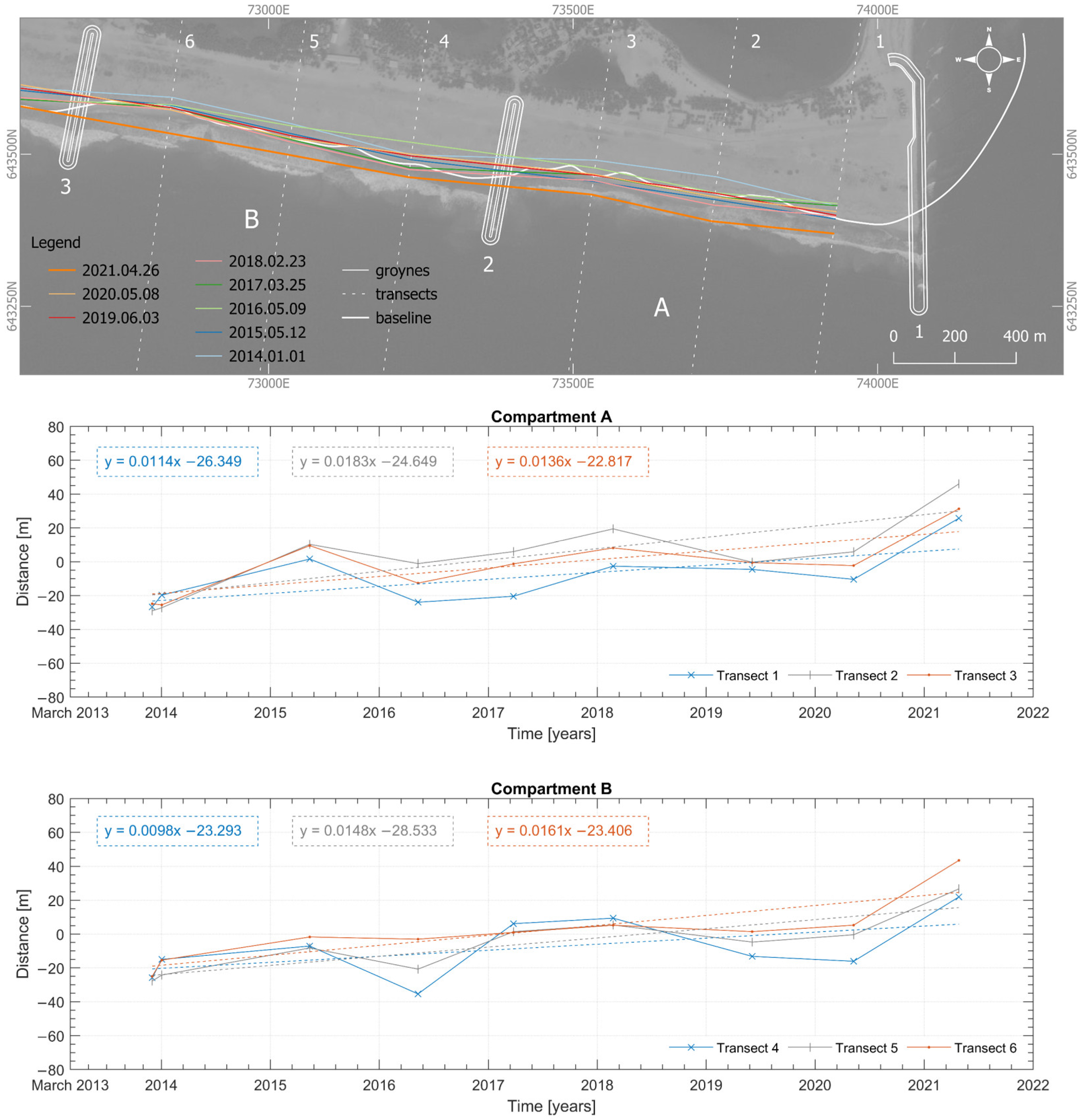
The recent shoreline evolution in the easternmost compartments (A and B) of the case study, near the Volta River Delta, is shown in Figure 7. Even though fluctuations around the reference shoreline are observed over the years, the shoreline evolution in these two compartments is overall positive. It is observed that in late November 2013 the shoreline position in these compartments is moderately to significantly retreated with respect to the reference shoreline. The nourishment brings this shoreline forward. Following construction, significant retreats are still observed in 2016 and 2020, with a maximum of −35 m in transect 4 of compartment B in 2016. The remainder of the observations indicate, however, only little to moderate retreats. The highest shoreline advance, circa +40 m, is observed in 2021 at transects 2 and 6.

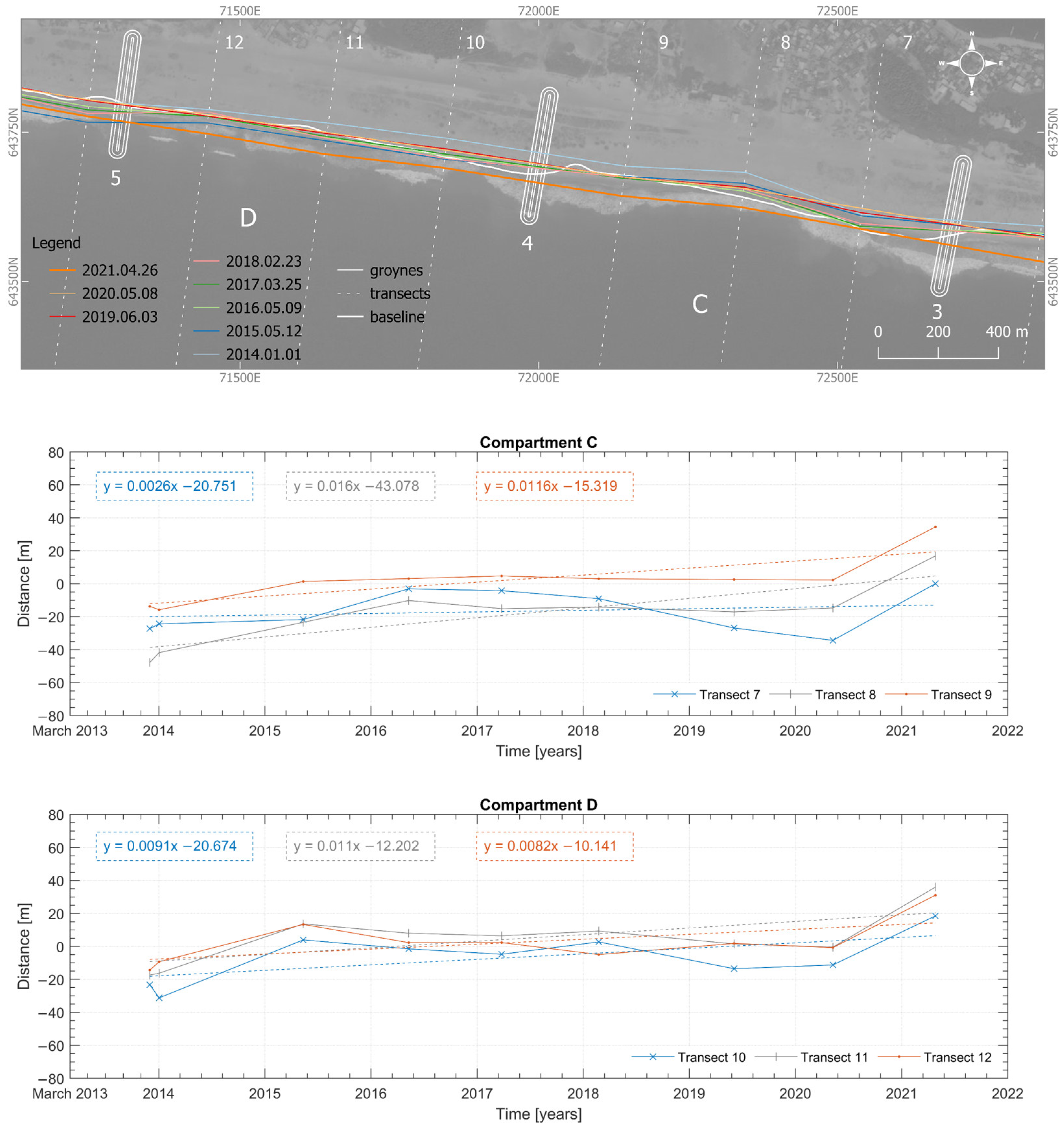
Shoreline evolution in compartments C and D (Figure 8) in the years of construction is very similar to that observed in easternmost compartments, i.e., retreat with respect to the reference prior to the nourishment works. In the immediate years following construction, up to 2017, the shoreline remained stable, and any changes were negligible. However, from 2017 to 2019, a steady retreat trend was observed. This trend is then reversed in 2021, following a sharp advance. Overall, the shoreline evolution trend in compartments C and D is positive. The largest shoreline advances (more than +30 m) were observed in transects 9, 11 and 12, while the largest moderate to significant retreats occurred in transects 7 and 10.

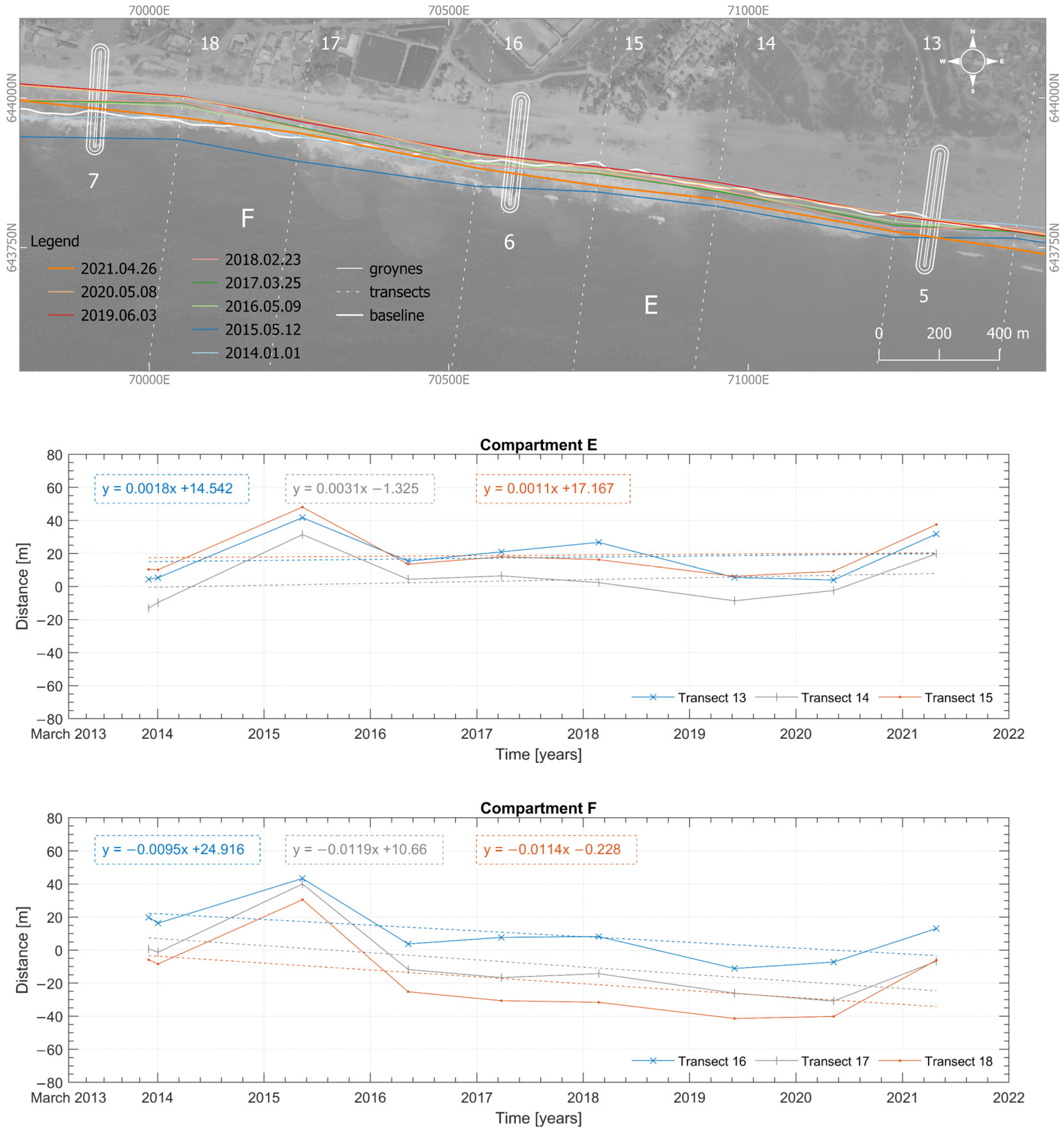
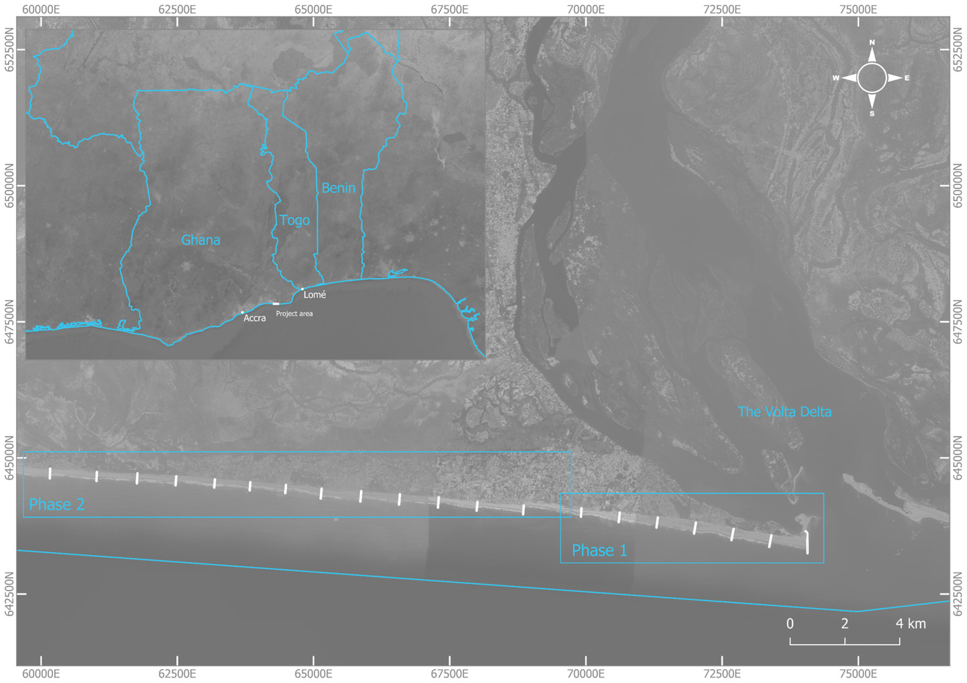
Contrarily to what is observed in the four easternmost compartments, there was no or only little shoreline retreat in late November 2013 in compartments E and F (Figure 9). In fact, for most of the transects considered in the analysis, the shoreline position was little to moderately advanced when compared to the reference. This is attributed to the accumulation of sediments in the updrift compartments of the groyne field, i.e., accumulation against groynes 6 and 7. It should be kept in mind that this is prior to the construction of Phase 2. Conversely, following the completion of the protection works in Phase 2, both compartments which are located immediately downdrift of the Phase 2 project area (Figure 1) started experiencing a sediment supply deficit. This resulted in an overall negative shoreline evolution, especially in compartment F. Although little to moderate, the observed shoreline evolution trend in compartment E remained positive over the period of analysis. The highest observed shoreline advances/retreats have similar orders of magnitude of those observed in the easternmost compartments.

Even though positive and negative fluctuations in the short-term shoreline evolution are observed within the beach compartments in Phase 1 following construction, the overall evolution trend is positive (advance) for the whole Phase 1, except in compartment F. As mentioned earlier, this is attributed to the location of compartment F immediately downdrift of the Phase 2 project area. Therefore, there is some expectation that the newly observed trend may be attenuated or even reversed in the coming years once more sand starts bypassing the groynes in Phase 2.

The shoreline evolution within compartment G (Figure 10), the easternmost in Phase 2, is very similar to that observed in compartment F in Phase 1, i.e., a steady shoreline retreat in the period of analysis. With respect to compartment H (Figure 10), no remarkable shoreline changes can be observed within the period of analysis, except those linked to the artificial beach nourishment works that took place here in March–April 2014.

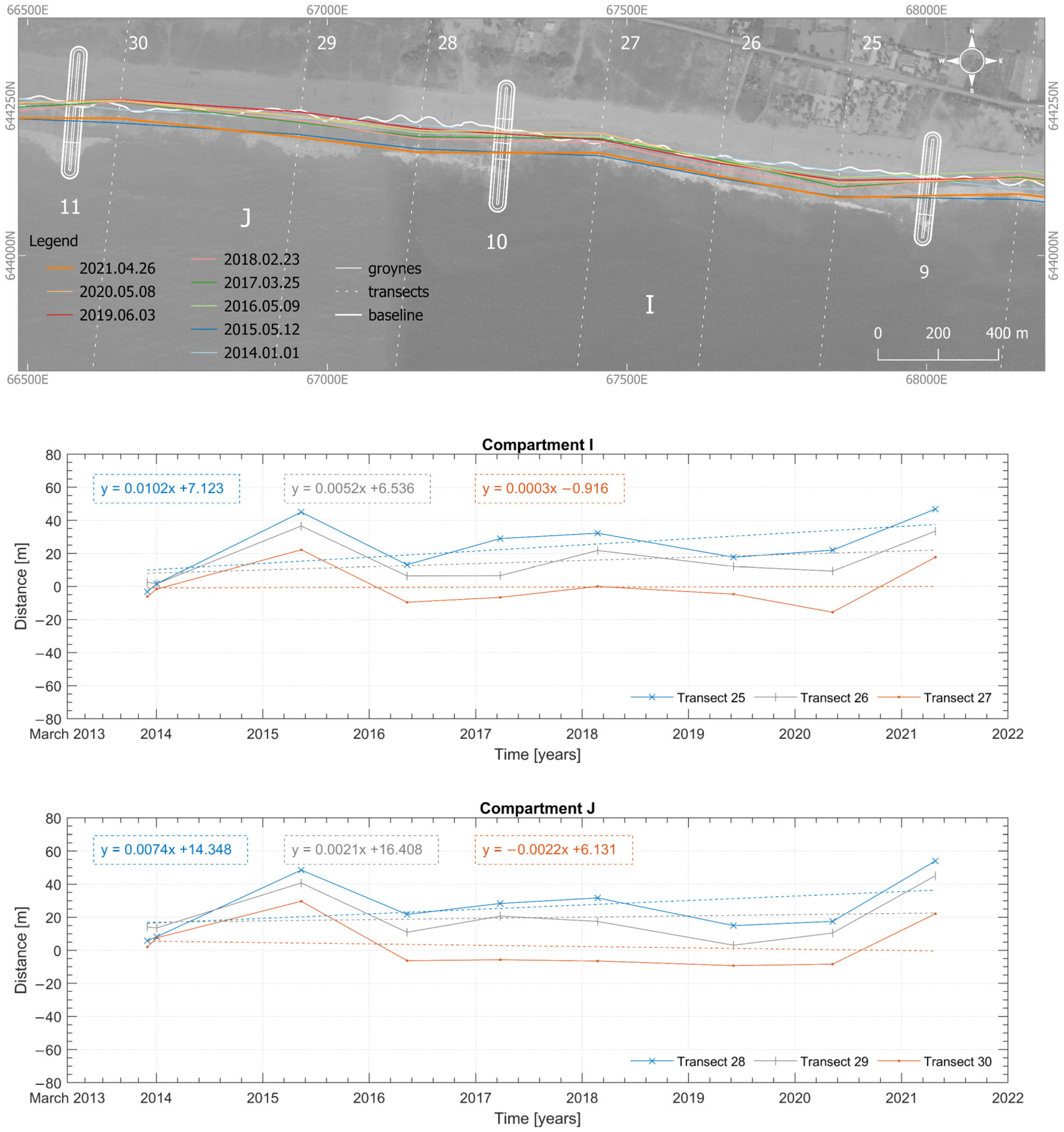
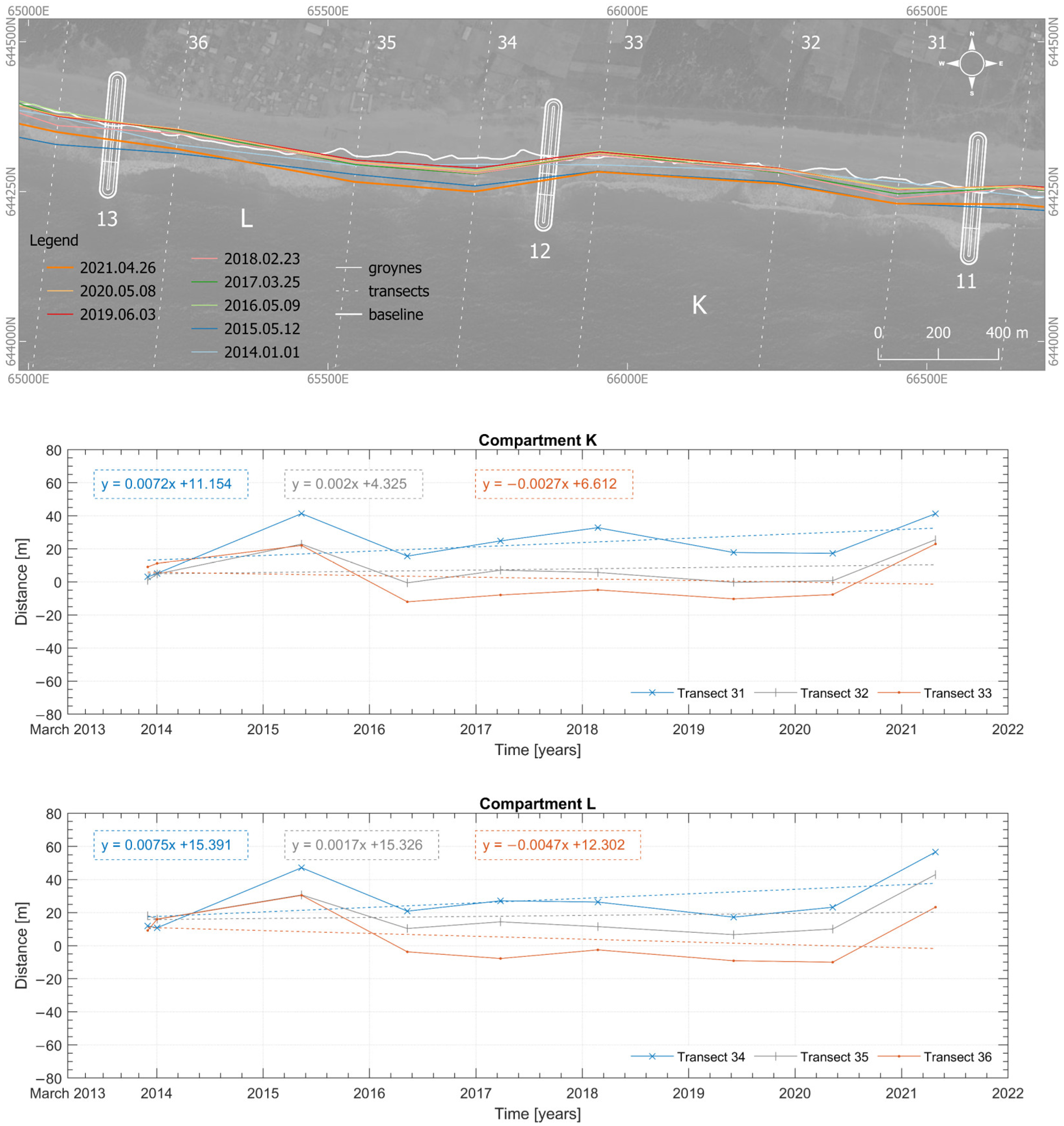
The shoreline evolutions within compartments I and J (Figure 11) and compartments K and L (Figure 11) are all in all similar within the period of analysis, that is, overall positive shoreline evolution with stable to little shoreline retreat trends downdrift of groynes. The orders of magnitude of the positive and negative fluctuations with respect to the reference line is as observed in other beach compartments. The largest positive advances in 2015 are associated with the nourishment works.

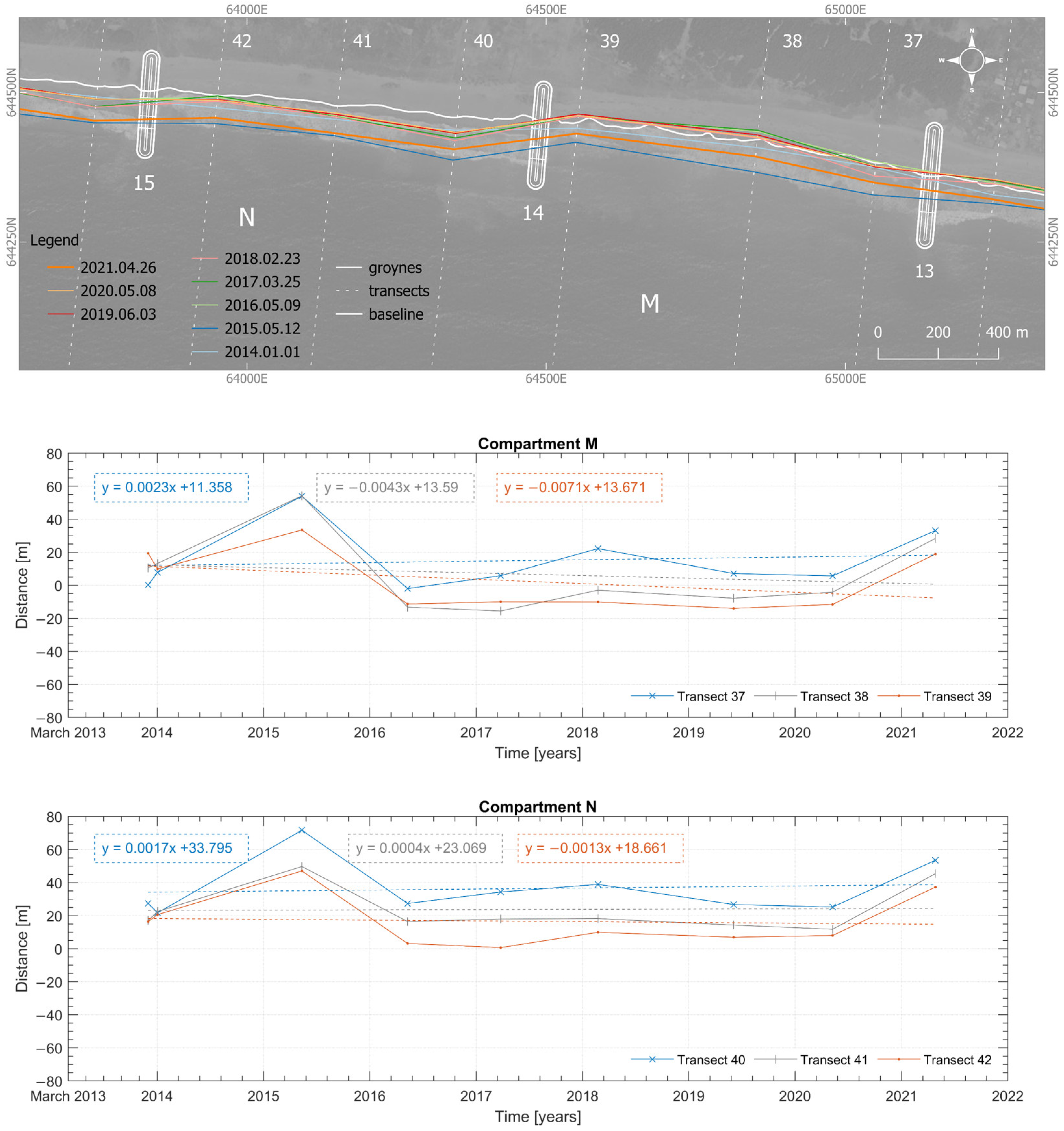
The shoreline within compartments M and N (Figure 13) remains generally stable following the coastal protection works. As noted in other compartments, significant shoreline advances are observed in 2015 following the nourishment works and again in 2021. The largest shoreline retreat (−16 m) in these compartments is observed in 2017 at transect 38 in compartment M. Within compartments M and N, downdrift erosion is more noticeable around groyne 14.

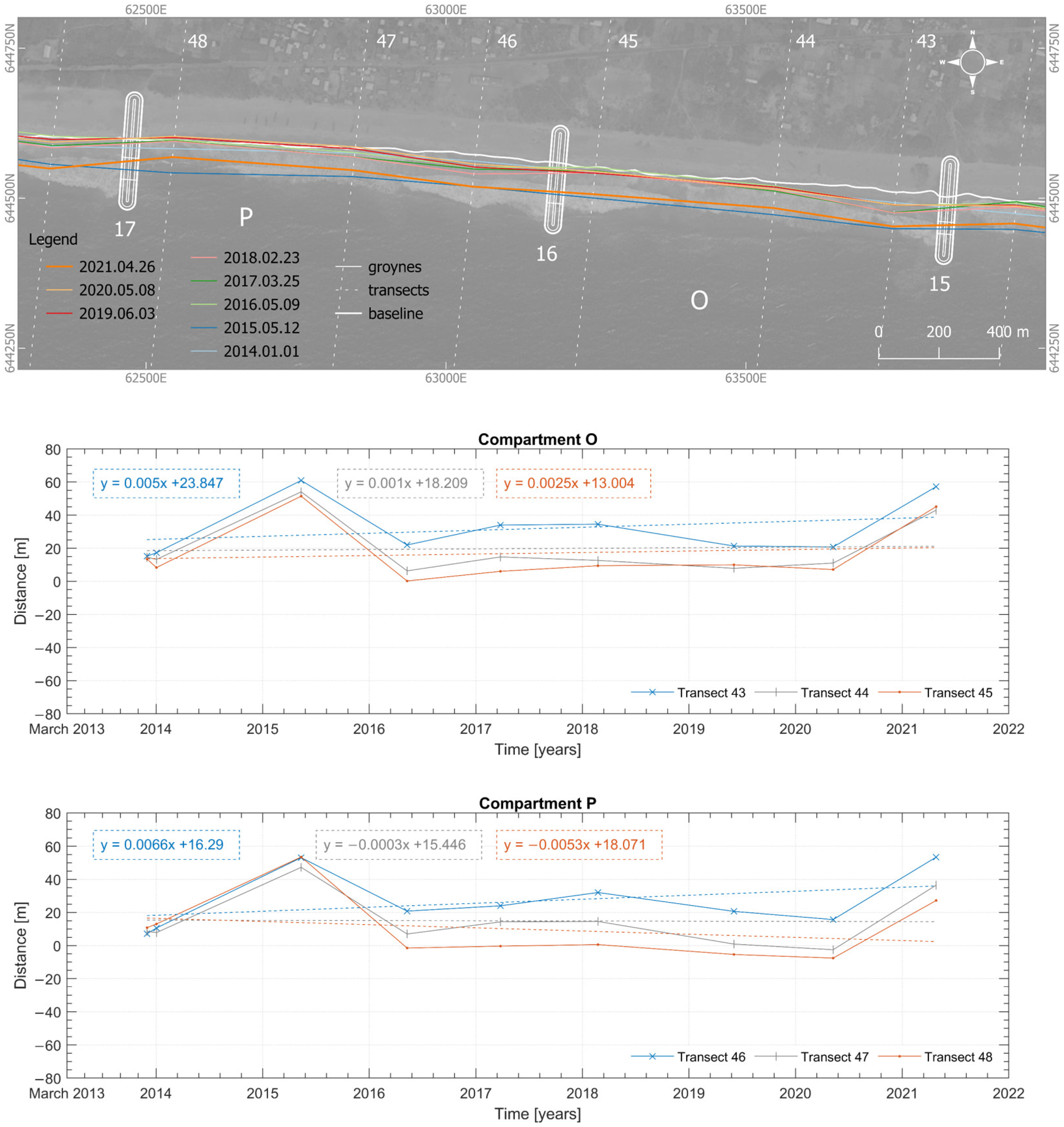
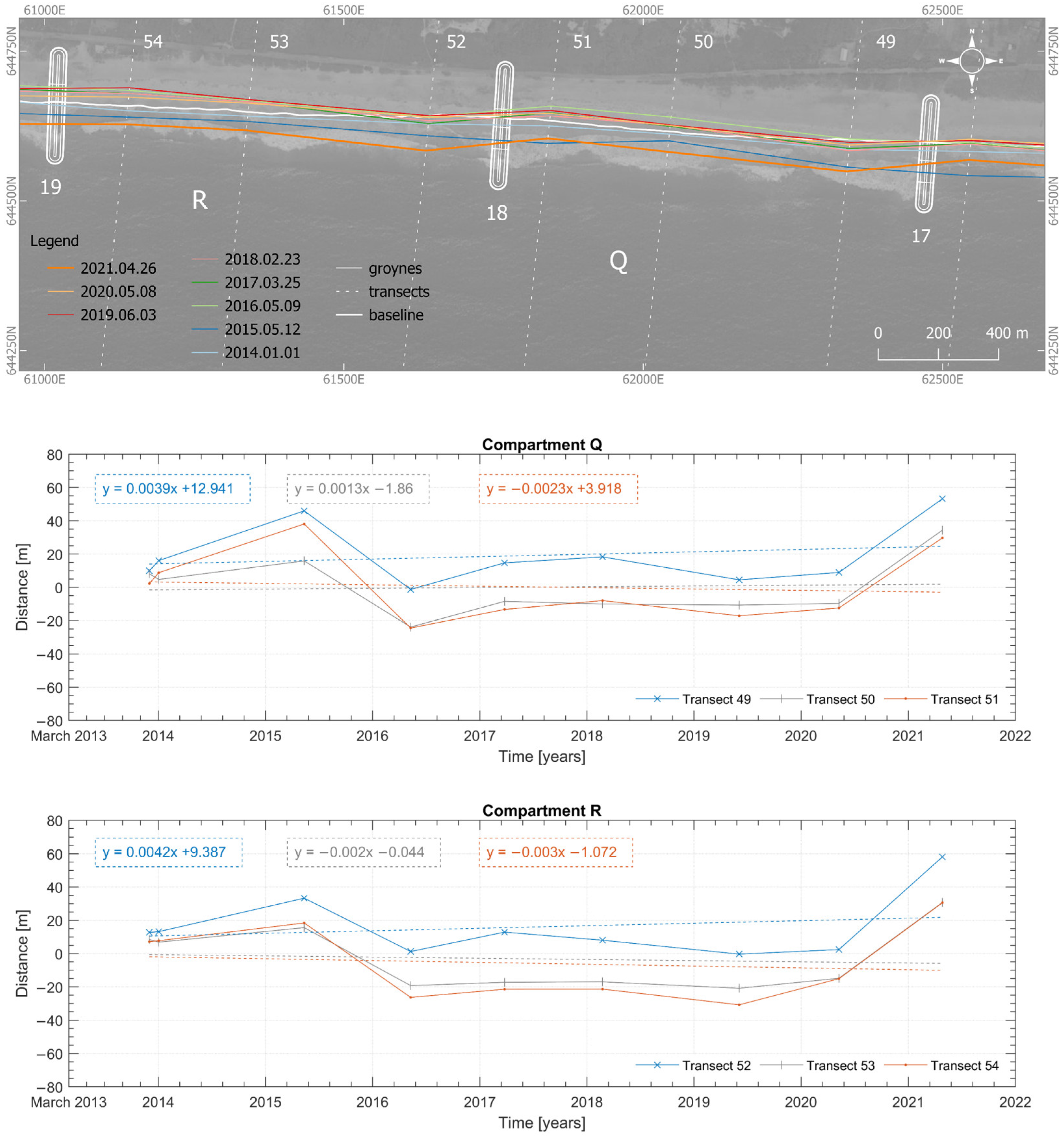
The trends observed in compartments O to S (Figure 14, Figure 15 and Figure 16) indicate that the shoreline position remains stable. Again, the largest shoreline advance occurred in 2015 following the nourishments, to which followed a large shoreline retreat in the year following construction. This is largely attributed to adjustments to the constructed beach profile resulting from the execution method. A significant advance was again observed in 2021.

Unsurprisingly, there is an overall positive trend in the westernmost compartments T (Figure 16) and U (Figure 17), with a steady significant shoreline advance since 2016. The large retreats observed in 2016 are largely attributed to adjustments to the constructed beach profile following construction. Based on the observed evolution, it is possible to state that in 2021 compartments T and U would be very close to their maximum sediment retention capacity. Natural sediment bypass in those compartments would thereby have been mostly re-established. It is anticipated that compartments downdrift will progressively also reach their maximum sediment retention capacity in the coming years.

Table 5. Summary of shoreline evolution trends per compartment along all transects. Red and green colours indicate retreat and advance, respectively; the colour gradation is according to the classification thresholds in Table 3; brackets indicate that a transect is observed to be stable.

	Transects	Trend [m/Year]		Transects	Trend [m/Year]
A	1	+4.2	L	34	+2.7
	2	+6.7		35	+0.6
	3	+5.0		36	−1.7
B	4	+3.6	M	37	+0.8
	5	+5.4		38	−1.6
	6	+5.9		39	−2.6
C	7	+0.9	N	40	+0.6
	8	+5.8		41	(+0.1)
	9	+4.2		42	−2.3
D	10	+3.3	O	43	+1.8
	11	+4.0		44	(+0.4)
	12	+3.0		45	+0.9
E	13	+0.7	P	46	+2.4
	14	+1.1		47	(−0.1)
	15	(+0.4)		48	−1.9
F	16	−3.5	Q	49	+1.4
	17	−4.3		50	(+0.5)
	18	−4.2		51	−0.8
G	19	−8.2	R	52	+1.5
	20	−9.3		53	−0.7
	21	−10.6		54	−1.1
H	22	+2.3	S	55	+2.0
	23	+1.8		56	(+0.3)
	24	−0.6		57	(+0.4)
I	25	+3.7	T	58	+7.2
	26	+1.9		59	+7.8
	27	(+0.1)		60	+7.2
J	28	+2.7	U	61	+7.2
	29	+0.8		62	+5.6
	30	−0.8		63	+6.8
K	31	+2.6		64	+4.0
	32	+0.7
	33	−1.0

presents a summary of the observed trends per transect in each compartment. Trends are classified according to the thresholds in Table 3.

Shoreline advance in all transects is observed in compartments A to E in Phase 1 and compartments I, O, and S to U in Phase 2. This is 46% of the entire project area. Furthermore, all transects in compartments A, B, D, T, and U evidenced significant shoreline advance, meaning the shoreline is advancing within these compartments at a yearly rate of more than +3 m/year on average. The largest advance rate, +7.8 m/year, is observed at the mid-point transect of compartment T. Conversely, transects in compartments F and G represent 11% of the entire project area, which evidenced significant shoreline retreat. The largest retreat rates, −8.2 to −10.6 m/year, are observed in beach compartment G.

In the remainder of the project area, there is evidence of little to moderate shoreline retreat at transects downdrift of groynes, while the other transects evidenced little to moderate shoreline advance. This is only observed in Phase 2 and can be attributed to the groynes being partially impermeable in Phase 2. Since this behaviour is mostly observed in groynes located further downdrift in the Phase 2 project area, it is likely that differences now observed between transects updrift and downdrift of groynes will be progressively attenuated as compartments reach their maximum retention capacity, based on what is already observed in compartments located further updrift (i.e., compartments S, T, and U).

To a greater or lower extent, an adjustment of the shoreline position was invariably observed in the year following the nourishment works. This sort of adjustment is typical in beach nourishment projects constructed by overbuilding, i.e., sand is placed on the beach following a much wider and much steeper beach profile than designed. It should be noted that the variable controlled during construction was the volume of sand deposited in each compartment. The expectation is that natural coastal processes will continue re-shaping the built beach profile towards the design profile.

4.2.2. Analysis of the Coastline Evolution Updrift and Downdrift of a Groyne

The shoreline evolution trends along the transect located updrift or downdrift of groynes are analysed in this section. This analysis focuses on the differences observed downdrift and updrift, as well as the changes in active length (i.e., length of the groyne extending from the shoreline seawards to groyne head) and how these changes may affect the recommended design ratios for groyne fields (e.g., the ratio of spacing between groynes to groyne length). 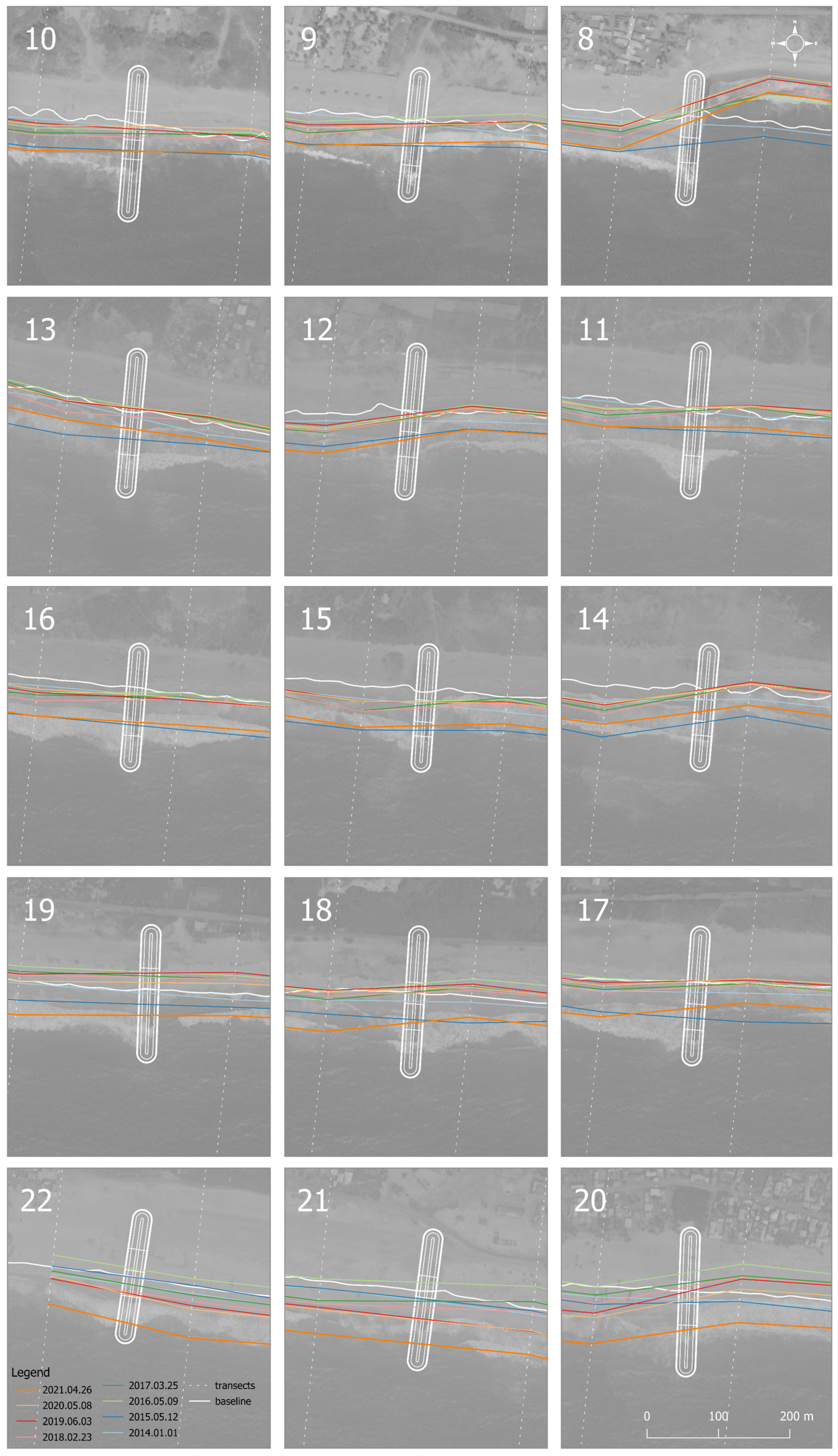Figure 18 and Figure 19 present a plan view of the shoreline positions around groyne locations over the period of analysis in Phase 1 and Phase 2, respectively.

The most noteworthy takeaway in Figure 18 is that there are no important differences between the updrift and downdrift sides of the groynes in Phase 1. Only minor and generally transient differences can be observed. Conversely, the groynes in the Phase 2 project area (Figure 19) show to a higher (e.g., groynes 8, 12, 14, and 20) or lower extent (e.g., groynes 13, 16, 21, and 22) marked differences between the shoreline position at the updrift and downdrift sides. This is attributed to the fact that the groynes in Phase 2 are partially impermeable and are, therefore, expected to experience some temporary leeside erosion before sediment bypass is re-established, as explained earlier. Based on the present analysis, this seems to have happened already at groynes 21 and 22, the westernmost in the entire project area and the most updrift considering the prevailing direction of the longshore drift current, which in Ghana is from the west to the east.

The distances of the extracted shorelines in 2015, 2016, 2020, and 2021 relative to the reference shoreline in March 2013 (baseline), updrift and downdrift of groynes, are presented in

Table 6. Distances of the extracted shorelines in 2015, 2016, 2020, and 2021 relative to the reference shoreline in March 2013 (baseline), updrift and downdrift groynes. Red and green colours indicate retreat and advance, respectively; the colour gradation is according to the classification thresholds in Table 4; brackets indicate that the updrift or the downdrift side is observed to be stable.

Distances [m]
Groyne	Updrift				Downdrift
	2015	2016	2020	2021	2015	2016	2020	2021
2	−7	−35	−16	+22	+9	−12	(−2)	+31
3	−21	(−3)	−33	(+1)	(−2)	(−3)	(+5)	+43
4	(+4)	(−1)	−11	+19	(+1)	(+3)	(+2)	+34
5	+41	+15	(+5)	+31	+13	(+3)	(−1)	+31
6	+43	(+4)	−7	+13	+47	+13	+10	+37
7	+47	−16	−40	−16	+31	−24	−39	−6
8	+59	+20	+25	+56	+22	−34	−63	−40
9	+45	+13	+22	+47	+28	−19	−7	+19
10	+48	+22	+18	+54	+22	−9	−16	+18
11	+41	+15	+17	+41	+30	−6	−8	+22
12	+46	+21	+23	+56	+22	−12	−7	+23
13	+54	(−2)	+6	+33	+30	(−4)	−10	+23
14	+71	+27	+25	+53	+34	−11	−11	+19
15	+60	+22	+21	+57	+47	(+3)	+9	+37
16	+53	+20	+15	+53	+51	(0)	+8	+45
17	+46	(−1)	+9	+53	+53	(−2)	−7	+27
18	+33	(+1)	(+2)	+57	+38	−24	−12	+30
19	+26	−21	(0)	+47	+18	−26	−15	+30
20	+24	(0)	+43	+79	+12	−41	(−5)	+42
21	+10	(−3)	+40	+74	(+3)	−31	+31	+64
22	(−1)	−16	+13	+52	(−2)	−12	+31	+71

. These distances are classified based on the thresholds discussed in Section 3.4 and presented in Table 4. In 2021, leeside erosion is noticeable only downdrift of groynes 7 and 8. For the remainder of the groynes, a moderate to significant advance is observed. Also in 2021, a significant advance (i.e., more than +30 m) is observed updrift of all groynes in Phase 2, whereas at the updrift side of groynes 2 to 6 in Phase 1 the shoreline is stable (updrift of groyne 3) or moderately (groynes 2, 4, and 6) to significantly (groyne 5) advancing. Updrift of groyne 7 in Phase 1, the shoreline is moderately retreating. Even though there are important oscillations of the shoreline position across the period under analysis, the observations around groynes support the discussion in previous sections, i.e., some leeside erosion is observed following construction, slowly attenuated by the sand accumulating inside the beach compartments.

Table 7. Evolution of the active lengths of the groynes across the period of analysis.

Groyne	Baseline (2013)	2013	2014	2015	2016	2017	2018	2019	2020	2021
2	99	136	132	110	135	109	102	118	120	85
3	89	122	115	107	100	98	97	108	110	74
4	73	103	109	81	83	84	82	90	89	58
5	79	82	80	48	70	65	62	77	78	50
6	72	56	58	28	66	62	63	78	75	52
7	59	49	49	15	73	75	78	95	92	63
8	118	-	-	72	119	116	117	130	131	104
9	101	-	-	66	105	92	93	97	95	70
10	124	-	-	87	116	110	106	117	120	86
11	107	-	-	82	113	110	108	114	115	87
12	110	-	-	75	106	101	99	107	102	72
13	106	-	-	68	114	112	100	112	113	82
14	98	-	-	55	100	97	94	101	100	71
15	98	-	-	45	85	80	76	85	84	51
16	104	-	-	51	95	91	86	90	94	55
17	103	-	-	53	105	98	96	104	104	67
18	106	-	-	68	116	106	105	113	109	63
19	90	-	-	69	114	109	106	113	100	54
20	106	-	-	90	133	118	112	106	95	52
21	99	-	-	88	110	84	75	59	59	24
22	82	-	-	81	92	69	60	57	56	17

presents the estimated active lengths of the groynes relative to the baseline and its evolution following construction. The active lengths are used to estimate the ratio of spacing between groynes to length with respect to the reference shoreline position and how this ratio has evolved since construction across the period of analysis. The purpose is to analyse how the initial ratio may have influenced the performance of the groynes.

According to the groynes’ design rules, the recommended spacing to length ratio is in between 1:3 and 1:4. This recommendation was ensured in all compartments (

Table 8. Evolution of the spacing to length ratio from design conditions to observed in 2021.

Compartments	Spacing between Groynes [m]	Spacing to Length Ratio
		Design Conditions	Observed in 2021
A	657	1:3	1:8
B	672	1:3	1:9
C	668	1:3	1:11
D	673	1:3	1:13
E	671	1:4	1:13
F	673	1:4	1:11
G	1030	1:6	1:9
H	824	1:5	1:11
I	685	1:3	1:8
J	687	1:3	1:8
K	681	1:3	1:9
L	700	1:4	1:9
M	628	1:4	1:9
N	628	1:4	1:12
O	623	1:4	1:11
P	681	1:4	1:11
Q	683	1:4	1:11
R	715	1:4	1:13
S	830	1:4	1:16
T	656	1:4	1:27
U	608	1:4	1:35

), except in G and H for the reasons already mentioned.

Following construction, the spacing to length ratio is expected to reduce while sediment accumulates against the groynes, thereby reducing the active length of the groynes. Hence, the sediment retention capacity within a beach compartment slowly reduces. In other words, there is a reduction in the groynes’ efficiency with respect to their capacity to retain more sand with time, because their maximum retention capacity is attained.

The results of the evolution of the spacing to length ratio from the design to 2021 are presented in Table 8. The evolution observed for this ratio shows that it was significantly smaller in 2021 compared to 2013, demonstrating the good performance of the designed groyne field. This observation is noted even in the beach compartments that started with a less favourable condition initially.

5. Conclusions

Satellite remote sensing can provide coastal managers with valuable information on ongoing coastal processes and major trends in coastline evolution, especially in data-poor regions. In this paper, the use of optical satellite images to map changes in shoreline position before and after the implementation of a coastal protection scheme is explored based on a case study located in the Greater Accra Region of Ghana. The case study investigated concerns a project for protecting people and livelihoods in Ada Foah and surrounding villages, which involved the implementation of 22 slope-crested groynes and the placement of 5 million cubic metres of sand (measured at the hopper) as artificial beach nourishment.

The monitoring through satellite remote sensing showed evidence that before implementation of the coastal protection scheme, the overall trend in this coastal stretch was of retreat (–1.6 m/year), which is in line with the average retreat rate of −1 to −2 m/year reported in the literature. Following the project, this trend was reversed, and the coast is now advancing at about +1 m/year.

Satellite-based monitoring of the project area over a period of about 9 years, between 2013 and 2021 (i.e., during construction work and after its completion), allowed for a better understanding of the major trends in coastline evolution following the implementation of the project. For example, apart from a few beach compartments mainly located downdrift of the Phase 2 project area, the shoreline position is experiencing a moderate (i.e., +1 to +3 m/year) to significant (more than +3 m/year) advance rate compared to the reference shoreline in March 2013 (baseline).

Unsurprisingly, given that the prevailing direction of the longshore drift current in Ghana is from the west to the east, the largest advance rates (more than +6 m/year on average) are observed in the westernmost beach compartments, compartments U and T. Significant advance rates are also observed in the easternmost compartments in the Phase 1 project area (i.e., compartments A to E), which may indicate that some of the sediments being removed in beach compartments F and G (the westernmost compartment in Phase 1 and the easternmost compartment in Phase 2, respectively) are being transported and retained further downdrift.

Coastal monitoring in Ada from earth-observing satellites also evidence positive and negative oscillations in the short-term shoreline evolution within the beach compartments over the years. Because the overall trend in this coastal stretch following the coastal protection works is of advancing, is possible to conclude that sediments are being captured within the beach compartments between groynes. Furthermore, it seems that sediment bypass has been re-established in the two westernmost compartments, indicating that these may have reached their maximum sediment retention capacity. This might gradually be observed also in compartments further downdrift. Therefore, monitoring should be continued in the coming years.

Furthermore, the analysis of the shoreline-extracted position based on satellite imagery also proved useful in assessing temporary leeside erosion following construction. For example, the assessment of the evolution of the shoreline position, updrift and downdrift of groynes, allowed a clear identification of the impact of the differences in the permeability of groynes in Phase 1 and in Phase 2. Specifically, while no important differences between the updrift and downdrift sides of the Phase 1 groynes are observed, some differences could be identified in Phase 2. This is because the groynes in Phase 2 are partially impermeable and will therefore experience some temporary leeside erosion before sediment bypass is re-established. This seems to have happened already at the westernmost groynes 21 and 22, as well as in some other groynes in the Phase 2 project area where less difference between the two sides is noticeable. It is, however, too early to draw any conclusion on this.

Finally, monitoring through satellite remote sensing can be used to confirm widely used rules of thumb when designing groyne fields. In this paper, one such rule of thumb—the spacing to length ratio—has been investigated. More specifically, the paper discusses the evolution of this ratio as a predictor for the performance of groyne fields. In the Ada project, this ratio was observed to be reducing with the reduction in the groynes’ active length due to the sedimentation within the beach compartments.

References

1. Kulp, S.A.; Strauss, B.H. New elevation data triple estimates of global vulnerability to sea-level rise and coastal flooding. Nat. Commun. 2019, 10, 4844. [Google Scholar] [CrossRef]
2. Luijendijk, A.; Hagenaars, G.; Ranasinghe, R.; Baart, F.; Donchyts, G.; Aarninkhof, S. The State of the World’s Beaches. Sci. Rep. 2018, 8, 6641. [Google Scholar] [CrossRef] [PubMed]
3. Lo, A.Y.; Liu, S.; Cheung, L.T.O.; Chan, F. Synergies and Trade-Offs Between Sustainable Economic Development and Climate Change Adaptation; GAR2022 Contributing Paper; United Nations Office for Disaster Risk Reduction: Geneva, Switzerland, 2022. Available online: www.undrr.org/GAR2022 (accessed on 8 September 2023).
4. das Neves, L.; Bolle, A.; De Nocker, L. Cost-benefit-analysis of coastal adaptation strategies and pathways. A case study in West Africa. Ocean Coast. Manag. 2023, 239, 106576. [Google Scholar] [CrossRef]
5. Vitousek, S.; Buscombe, D.; Vos, K.; Barnard, P.; Ritchie, A.; Warrick, J. The future of coastal monitoring through satellite remote sensing. Camb. Prisms Coast. Futures 2023, 1, E10. [Google Scholar] [CrossRef]
6. De Schipper, M.A.; de Vries, S.; Ruessink, G.; de Zeeuw, R.C.; Rutten, J.; van Gelder-Maas, C.; Stive, M.J. Initial spreading of a mega feeder nourishment: Observations of the sand engine pilot project. Coast. Eng. 2016, 111, 23–38. [Google Scholar] [CrossRef]
7. Castelle, B.; Bujan, S.; Marieu, V.; Ferreira, S. 16 years of topographic surveys of rip-channelled high-energy meso-macrotidal sandy beach. Sci. Data 2020, 7, 410. [Google Scholar] [CrossRef] [PubMed]
8. Turner, I.L.; Harley, M.D.; Short, A.D.; Simmons, J.A.; Bracs, M.A.; Phillips, M.S.; Splinter, K.D. A multi-decade dataset of monthly beach profile surveys and inshore wave forcing at Narrabeen, Australia. Sci. Data 2016, 3, 160024. [Google Scholar] [CrossRef]
9. Ludka, B.C.; Guza, R.T.; O’Reilly, W.C.; Merrifield, M.A.; Flick, R.E.; Bak, A.S.; Hesser, T.; Bucciarelli, R.; Olfe, C.; Woodward, B.; et al. Sixteen years of bathymetry and waves at San Diego beaches. Sci. Data 2019, 6, 161. [Google Scholar] [CrossRef] [PubMed]
10. Willis, C.P.; Griggs, G.B. Delineating Long-Term Trends in Beach Change, Central California. In California and the World Ocean ‘02: Revisiting and Revising California’s Ocean Agenda; American Society of Civil Engineers: Reston, VA, USA, 2012. [Google Scholar]
11. Hapke, C.J.; Reid, D.; Richmond, B.M.; Ruggiero, P.; List, J. National Assessment of Shoreline Change Part 3: Historical Shoreline Change and Associated Coastal Land Loss Along Sandy Shorelines of the California Coast. U.S. Geological Survey, Open File Report 2006-1219. 2012. Available online: https://pubs.usgs.gov/of/2006/1219/ (accessed on 8 September 2023).
12. Taveira-Pinto, F.; Henriques, R.; Rosa-Santos, P.; Fazeres-Ferradosa, F.; das Neves, L.; Pinto, F.V.C.T.; Sarmento, M.F. Hazard mapping based on observed coastal erosion rates and definition of set-back lines to support coastal management plans in the north coast of Portugal. J. Integr. Coast. Zone Manag. 2022, 22, 225–239. [Google Scholar] [CrossRef]
13. Bolle, A.; das Neves, L.; Rooseleer, J. Coastal protection for Ada, Ghana: A case study. Proc. Inst. Civ. Eng. Marit. Eng. 2015, 168, 125–133. [Google Scholar] [CrossRef]
14. The World Bank. West Africa Coastal Areas Management Program. 2016. Available online: https://www.wacaprogram.org/ (accessed on 8 September 2023).
15. Barbière, J. Coastal Erosion Major Threat to West-Africa. 2012. Available online: http://www.unesco.org/new/en/havana/about-this-office/single-view-havana/news/coastal_erosion_major_threat_to_west_africa/#.Vp9pt_lsOUk (accessed on 13 February 2017).
16. Charuka, B.; Angnuureng, D.B.; Agblorti, S.K.M. Mapping and assessment of coastal infrastructure for adaptation to coastal erosion along the coast of Ghana. Anthr. Coasts 2023, 6, 11. [Google Scholar] [CrossRef]
17. Campbell, M.O. The Sustainability of Coconut Palm Cocos nucifera Linnaeus 1753 Groves in Coastal Ghana. J. Coast. Res. 2006, 22, 1118–1124. [Google Scholar] [CrossRef]
18. Bolle, A.; das Neves, L.; De Nocker, L.; Dastgheib, A.; Couderé, K. A methodological framework of quantifying the cost of environmental degradation driven by coastal flooding and erosion: A case study in West Africa. Int. J. Disaster Risk Reduct. 2021, 54, 102022. [Google Scholar] [CrossRef]
19. Kusimi, J.M.; Dika, J.L. Sea erosion at Ada Foah: Assessment of impacts and proposed mitigation measures. Nat. Hazards 2012, 64, 983–997. [Google Scholar] [CrossRef]
20. Boateng, I. An application of GIS and coastal geomorphology for large scale assessment of coastal erosion and management: A case study of Ghana. J. Coast. Conserv. 2012, 16, 383–397. [Google Scholar] [CrossRef]
21. Allersma, E.; Tilmans, W.M.K. Coastal conditions in West Africa—A review. Ocean Coast. Manag. 1993, 19, 199–240. [Google Scholar] [CrossRef]
22. Jonah, F.E.; Adjei-Boateng, D.; Agbo, N.W.; Mensah, E.A.; Edziyie, R.E. Assessment of sand and stone mining along the coastline of Cape Coast, Ghana. Ann. GIS 2015, 21, 223–231. [Google Scholar] [CrossRef]
23. Boateng, I.; Wiafe, G.; Jayson-Quashigah, P.-N. Mapping Vulnerability and Risk of Ghana’s Coastline to Sea Level Rise. Mar. Geod. 2017, 40, 23–39. [Google Scholar] [CrossRef]
24. Vos, K.; Splinter, K.D.; Harley, M.D.; Simmons, J.A.; Turner, I.L. CoastSat: A Google Earth Engine-enabled Python toolkit to extract shorelines from publicly available satellite imagery. Environ. Model. Softw. 2019, 122, 104528. [Google Scholar] [CrossRef]
Figure 1. Ada Coastal Protection Works, project location, Phase 1 and Phase 2.
Jmse 11 01771 g001
Figure 2. Division of the case study area in beach compartments (identified by letters from A in the east to U in the west) between two adjacent groynes (identified with numbers from 1 in the east to 22 in the west).
Jmse 11 01771 g002
Figure 3. Methodology workflow.
Jmse 11 01771 g003
Figure 4. Examples of observed anomalies in satellite imagery of the case study area in 1985 (left panel), and 2010 (right panel) [source: Google Earth].
Jmse 11 01771 g004
Figure 5. Distances along transects of the extracted shorelines to the reference (March 2013), after artificial nourishment during the study period.
Jmse 11 01771 g005
Figure 6. Distances along transects of the extracted shorelines to the reference (March 2013) during and following construction.
Jmse 11 01771 g006
Figure 7. Groyne compartments A and B (including groynes 1, 2, and 3) and distance to the reference shoreline (2013) per considered transect.
Jmse 11 01771 g007
Figure 8. Groyne compartments C and D (including groynes 3, 4, and 5) and distance to the reference shoreline (2013) per considered transect.
Jmse 11 01771 g008
Figure 9. Groyne compartments E and F (including groynes 5, 6, and 7) and distance to the reference shoreline (2013) per considered transect.
Jmse 11 01771 g009
Figure 10. Groyne compartments G and H (including groynes 7, 8, and 9) and distance to the reference shoreline (2013) per considered transect.
Jmse 11 01771 g010
Figure 11. Groyne compartments I and J (including groynes 9, 10, and 11) and distance to the reference shoreline (2013) per considered transect.
Jmse 11 01771 g011
Figure 12. Groyne compartments K and L (including groynes 11, 12, and 13) and distance to the reference shoreline (2013) per considered transect.
Jmse 11 01771 g012
Figure 13. Groyne compartments M and N (including groynes 13, 14, and 15) and distance to the reference shoreline (2013) per considered transect.
Jmse 11 01771 g013
Figure 14. Groyne compartments O and P (including groynes 15, 16, and 17) and distance to the reference shoreline (2013) per considered transect.
Jmse 11 01771 g014
Figure 15. Groyne compartments Q and R (including groynes 17, 18, and 19) and distance to the reference shoreline (2013) per considered transect.
Jmse 11 01771 g015
Figure 16. Groyne compartments S and T (including groynes 19, 20, and 21) and distance to the reference shoreline (2013) per considered transect.
Jmse 11 01771 g016
Figure 17. Groyne compartment U (including groynes 21 and 22) and distance to the reference shoreline (2013) per considered transect.
Jmse 11 01771 g017
Figure 18. Coastline evolution updrift and downdrift the groynes of Phase 1 with respect to the reference shoreline of 2013 (i.e., baseline). The groyne number is indicated on the top left corner.
Jmse 11 01771 g018
Figure 19. Coastline evolution updrift and downdrift the groynes of Phase 2, against reference shoreline in 2013 (i.e., baseline). The groyne number is indicated on the top left corner.
Jmse 11 01771 g019