The Hydrodynamic Interaction between an AUV and Submarine during the Recovery Process

Abstract

The hydrodynamic interaction between an AUV (Autonomous Underwater Vehicle) and a recovery device, such as a real-scale submarine, is a crucial factor affecting the safe recovery of the AUV. This paper employs the CFD (Computational Fluid Dynamics) method to investigate the hydrodynamic interaction of the AUV and the submarine during the recovery process. Both the AUV and the submarine are considered to be relatively stationary. The results indicate that the submarine has a significant impact on the AUV during the recovery process, with sailing speed and relative positions identified as key influential factors. Due to the influence of the submarine, it can be difficult for the AUV to approach the submarine and be recovered safely. This study provides valuable insights into the hydrodynamic interaction between the AUV and the recovery device, and offers guidance for future submarine recovery operations involving AUVs. By considering the influence of the submarine’s position and motion, as well as other relevant factors, it may be possible to improve the stability, safety, and efficiency of AUV recovery operations.

1. Introduction

Autonomous Underwater Vehicles (AUVs) have gained widespread applications in various fields, including bathymetry, environmental monitoring, underwater operations, and antimine activities, owing to their remarkable benefits [1,2,3]. However, with the increasing demand for AUV utilization, it is crucial to enhance their performance by increasing their underwater operation time, work efficiency, and endurance [4].

The recovery of an AUV after completing its mission is a critical aspect of AUV operation, as it requires energy replenishment, data processing, and maintenance [5,6]. Over the years, researchers have proposed various methods for recovering AUVs, which can be broadly classified into two categories: surface mother-ship recovery and underwater docking recovery [7,8,9]. Surface mother-ship recovery typically involves the AUV returning to a predetermined area and approaching the mother ship for recovery, where it is lifted using cranes and other equipment onboard the surface vessel [10,11,12]. More recently, unmanned surface vehicles (USVs) have been used in the recovery process, providing a flexible and efficient solution for AUV recovery [13]. Underwater docking recovery involves various methods and equipment, including capture rod docking [14], guided docking [15,16], seated docking [17], and docking recovery through the torpedo launch tube of submarines [18,19,20].

The hydrodynamic interaction between the AUV and recovery device is a crucial factor that must be taken into consideration during the recovery process [21,22]. The hydrodynamic interaction can have varying degrees of impact on the recovery process, including issues such as long recovery time, failure of recovery, and even collisions between the AUV and recovery device. As such, it is essential to study the hydrodynamic interaction between the AUV and recovery device to ensure a successful and safe recovery process. This requires taking into account several factors, such as the size and shape of the AUV, the hydrodynamic characteristics of the recovery device, and the surrounding water currents.

The hydrodynamic interaction during the AUV recovery process has indeed garnered the interest of numerous researchers, and significant work has been devoted to understanding this issue. One notable contribution to this field was made by Molland [23,24], who conducted an extensive investigation into the viscous interaction between a pair of ellipsoids in close proximity. This included low-speed wind tunnel experiments and numerical simulations, which considered the effects of various factors, such as the Reynolds number and the transverse distance between the ellipsoids on the drag and side force of a single ellipsoid. The results of this work have enhanced our knowledge of viscous interactions between two objects and provided valuable reference points for basic CFD algorithms. Other researchers, such as Husaini [25], Zhang [26], and Rattanasiri [27], have focused on studying the hydrodynamic interaction between AUV formations. Zhang’s research analyzed a range of factors that might impact the hydrodynamic interaction between AUVs, such as spacing, drift angle, appendages, and formation structure. Rattanasiri’s study, on the other hand, focused on the detailed analysis of the influence of the relative positioning between AUVs on the hydrodynamic interaction, dividing the dominant space around the AUV into seven areas based on drag.

Research on the hydrodynamic issues related to AUV docking has also received significant attention from researchers [28,29]. Wu et al. [30] investigated the docking of AUVs to a cone-shaped dock, considering various factors, such as different velocities, accelerations, dock shapes, gliding modes, cross currents from different directions, and rudder angles, in their simulations. Their findings indicated that an unclosed dock tends to decrease the drag of the AUV, and decelerating at a constant speed is beneficial for successful docking. Additionally, Meng et al. [31,32] conducted extensive research on the underwater docking of AUVs. This included exploring the influence of various docking methods and different structural forms of the docking device on the recovery process, as well as studying the hydrodynamic interaction between the AUV and the docking device when stationary and in motion. Their work has yielded important results, including the observation that installing the docking device in the middle of the submarine provides the best stability and that the AUV’s speed plays a vital role in the recovery process.

The hydrodynamic interaction between submarines and Unmanned Underwater Vehicles (UUVs) has been a focus of research for several years, and notable contributions have been made in this field. Fedor [33] studied the hydrodynamic interaction between a submarine and a much smaller UUV, attempting to identify an area around the submarine where the effect of hydrodynamic interaction on UUV launch and recovery is relatively small. His analysis considered the static situation of the submarine, and his results lacked experimental verification. Leong and Randeni [34,35,36] used CFD methods and captive model experiments to carry out steady-state analysis to estimate the hydrodynamic interaction effects on an AUV operating in proximity to a submarine. They considered the longitudinal and lateral positions of the AUV relative to the submarine and the diameter ratio between the AUV and the submarine. Their results indicated that the force/moment coefficients of the AUV due to hydrodynamic interaction were independent of the Reynolds number at test speeds within the fully turbulent regime, and the interaction effects are minimal around amidships of the submarine. Furthermore, Du [37] analyzed the variation of hydrodynamic coefficients of the AUV moving around a submarine by solving the Reynolds-Averaged Navier–Stokes (RANS) equation. His numerical results showed that the attack angles and sideslip angles of the AUV had a significant influence on hydrodynamic coefficients, while the effect of Reynolds numbers could be ignored.

Past studies on the hydrodynamic interaction between an AUV and submarines have primarily focused on the model size. However, in practical applications, the size of the submarine is significantly larger than that of the AUV. Thus, this paper seeks to address the hydrodynamic interaction between a full-sized submarine and an AUV. The commercial CFD software Siemens PLM STAR-CCM+16.02 was used to carry out this research. The submarine employed in this study was utilized as a recovery device and was magnified by 20 times from the full appendage SUBOFF model. This approach enabled us to capture the effects of a real-world-sized submarine on the hydrodynamic interaction with the AUV. Moreover, to enhance the realism of the simulation, the AUV shape used in this study is flat, unlike the traditional revolving body often used in previous research.

To provide a more comprehensive overview of the research conducted, the remainder of this paper is organized as follows. Section 2 provides an introduction to both the geometric and numerical models utilized in this study. In Section 3, we verify the numerical method employed in our research. Next, in Section 4, we analyze the hydrodynamic interaction between the AUV and submarine when they are relatively stationary, with consideration given to various relative positions and speeds. Finally, we draw conclusions based on our findings in Section 5.

2. Geometric Models and Numerical Methodology

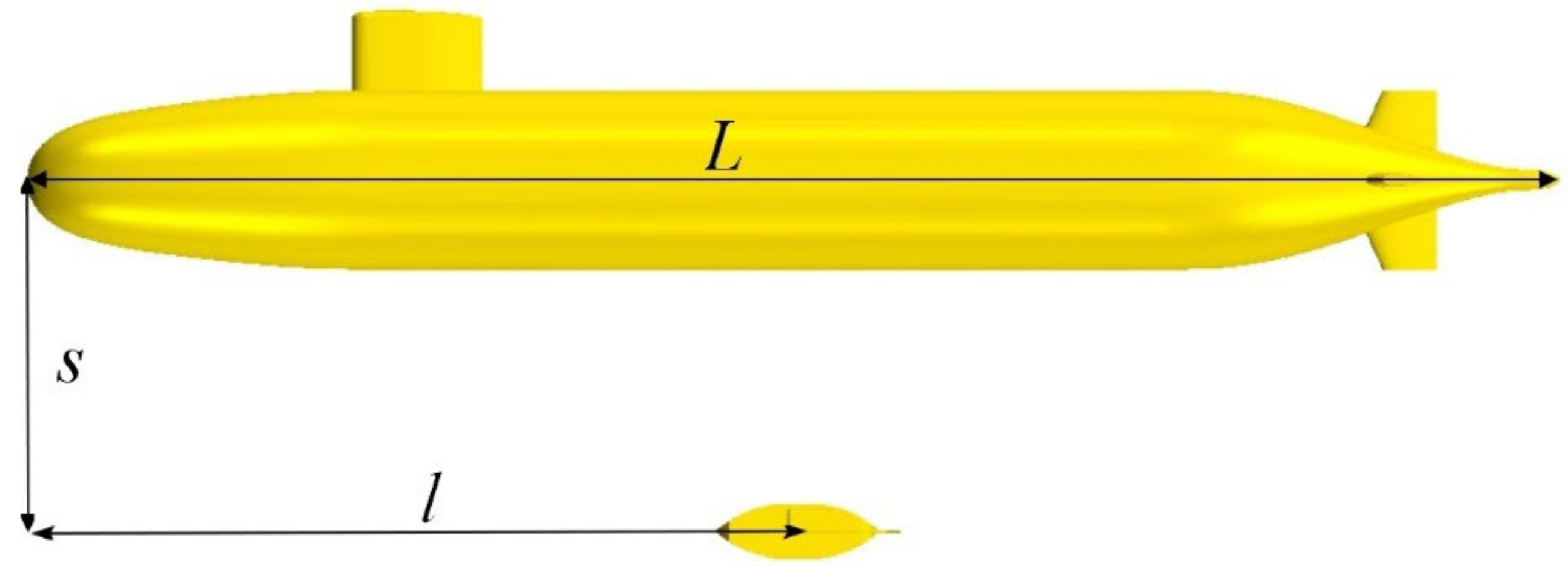
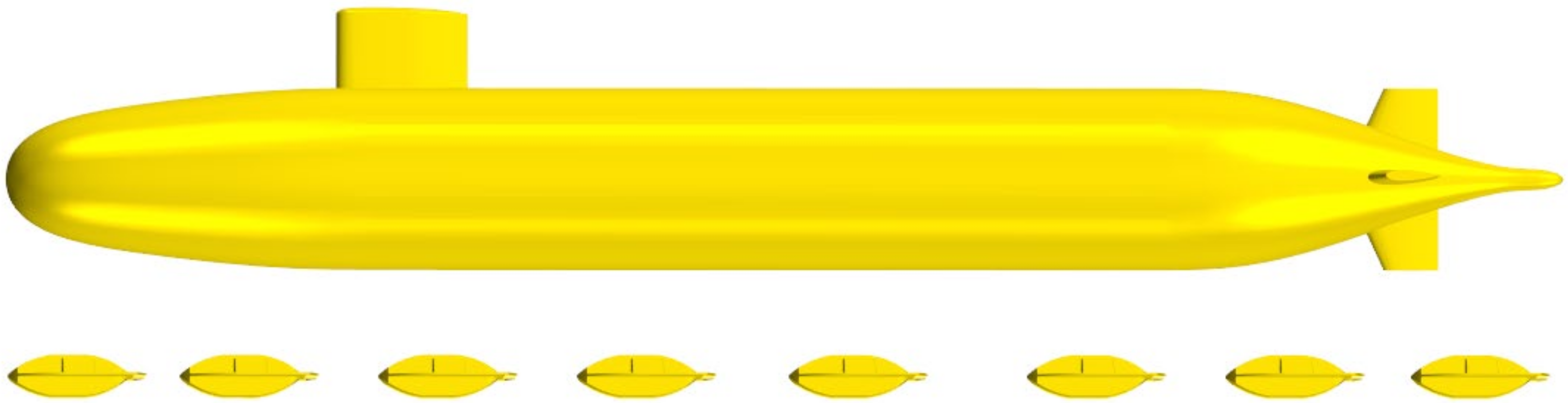
2.1. Geometric Models

The prototype of the submarine in this paper is the SUBOFF AFF-8 developed by DARPA (Defense Advanced Research Projects Agency) [38]. In order to approximate the size of the actual submarine, SUBOFF AFF-8 has been enlarged by 20 times. In addition, the AUV used in this paper is also different from the traditional AUV in the form of revolution. The geometry and main dimensions of SUBOFF and AUV are shown in Figure 1 and

Table 1. The main parameters for the SUBOFF model, the submarine, and AUV (m).

-	Length (m)	Radius/Width (m)	Height (m)
SUBOFF AFF-8	4.356 (LSUBOFF)	0.254 (RSUBOFF)	-
submarine	87.120 (Lsubmarine)	5.080 (Rsubmarine)	-
AUV	1.080 (LAUV)	0.923 (WAUV)	0.307 (HAUV)

, respectively. For convenience, the length of the SUBOFF AFF-8 and submarine are defined as L_SUBOFF and L_submarine, respectively. The length, width, and height of the AUV are defined as L_AUV, W_AUV, and H_AUV, respectively.

2.2. Numerical Methodology

2.2.1. Governing Equations and Numerical Setting

The CFD software utilized in this study is Siemens PLM STAR-CCM+16.02; the Reynolds-Averaged Navier–Stokes (RANS) equations discretized by the finite volume method (FVM) are applied to carry out the numerical simulation. The governing equations for unsteady, three-dimensional, incompressible flow are described below [39,40]:

$$\frac{\mathsf{\partial }{u}_i}{\mathsf{\partial }{x}_i}=0$$

(1)

$$\frac{\mathsf{\partial }{u}_i}{\mathsf{\partial }t}+\frac{\mathsf{\partial }\left(u_i{u}_j\right)}{\mathsf{\partial }{x}_j}=-\frac{\mathsf{\partial }P}{\mathsf{\partial }{x}_i}+\frac{\mathsf{\partial }}{\mathsf{\partial }{x}_j}\left[v\left(\frac{\mathsf{\partial }{u}_i}{\mathsf{\partial }{x}_j}+\frac{\mathsf{\partial }{u}_j}{\mathsf{\partial }{x}_i}\right)\right]-\frac{\mathsf{\partial }\overline{u_i^{’}{u}_j^{’}}}{\mathsf{\partial }{x}_j}$$

(2)

where $u_i$ and $x_i$ denote the velocity component and coordinate component in i direction, respectively; I = (1,2,3). P, v, and $-\overline{u_i^{’}{u}_j^{’}}$ are the static pressure, kinematic viscosity, and the Reynolds stress, respectively. ${\delta }_{ij}$ is the Kronecker delta, and the Reynolds stress is expressed as below:

$$-\overline{u_i^{’}{u}_j^{’}}=v_t\left(\frac{\mathsf{\partial }{u}_i}{\mathsf{\partial }{x}_j}+\frac{\mathsf{\partial }{u}_j}{\mathsf{\partial }{x}_i}\right)-\frac{2}{3}{\delta }_{ij}k$$

(3)

Here, $v_t=C_{\mu }{k}^2/\epsilon$ is the turbulent viscosity, where $C_{\mu }$ is an empirical number $(C_{\mu }=0.09$). k is the turbulent kinetic energy, and $\epsilon$ is the turbulent dissipation rate.

The k-$\epsilon$ turbulent model is applied to close the momentum equation; the two transport equations for k-$\epsilon$ are defined as:

$$\frac{\mathsf{\partial }k}{\mathsf{\partial }t}+\frac{\mathsf{\partial }\left(k{u}_j\right)}{\mathsf{\partial }{x}_j}=\frac{\mathsf{\partial }}{\mathsf{\partial }{x}_j}\left[\left(v+\frac{v_t}{{\sigma }_k}\right)\frac{\mathsf{\partial }k}{\mathsf{\partial }{x}_j}\right]+P_k-\epsilon$$

(4)

$$\frac{\mathsf{\partial }\epsilon }{\mathsf{\partial }t}+\frac{\mathsf{\partial }\left(k{u}_j\right)}{\mathsf{\partial }{x}_j}=\frac{\mathsf{\partial }}{\mathsf{\partial }{x}_j}\left[\left(v+\frac{v_t}{{\epsilon }_k}\right)\frac{\mathsf{\partial }\epsilon }{\mathsf{\partial }{x}_j}\right]+C_{\epsilon 1}{P}_k\frac{\epsilon }{k}-C_{\epsilon 2}\frac{{\epsilon }^2}{k}$$

(5)

In this study, spatial discretization employs second-order schemes for increased numerical accuracy. For temporal discretization, the first-order implicit Euler scheme is adopted, striking a balance between computational efficiency and accuracy in capturing time-dependent flow behavior. To solve the flow equations, a segregated flow solver based on the SIMPLE algorithm is implemented. This algorithm iteratively couples the pressure and velocity components to reach a converged solution. In each simulation, the time step size is determined using the Courant–Friedrichs–Lewy (CFL) condition, determined by CFL = U∆t/∆x, where U represents the characteristic velocity, ∆t is the time step size, and ∆x is the characteristic length scale. The Courant number is calculated for each cell and is typically kept below or equal to 1 for numerical stability. Finally, convergence is considered achieved when the forces acting on the submarine and AUV, the flow field, and the residual values reach a stable state. This indicates that the calculations have reached a reliable and consistent solution.

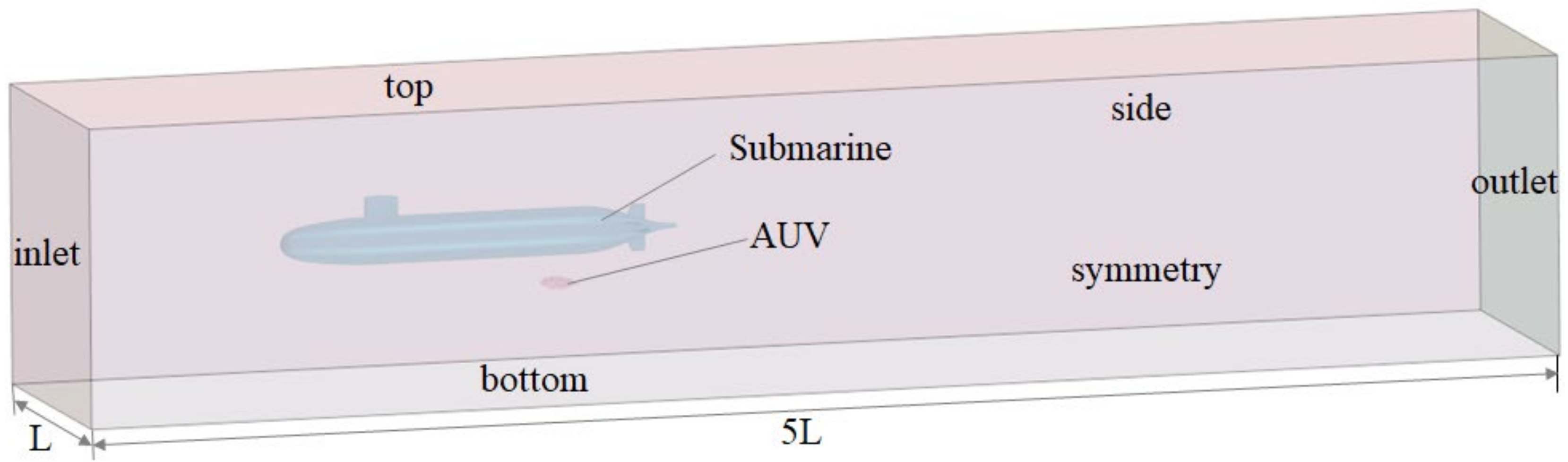
2.2.2. Fluid Domain and Boundary Conditions

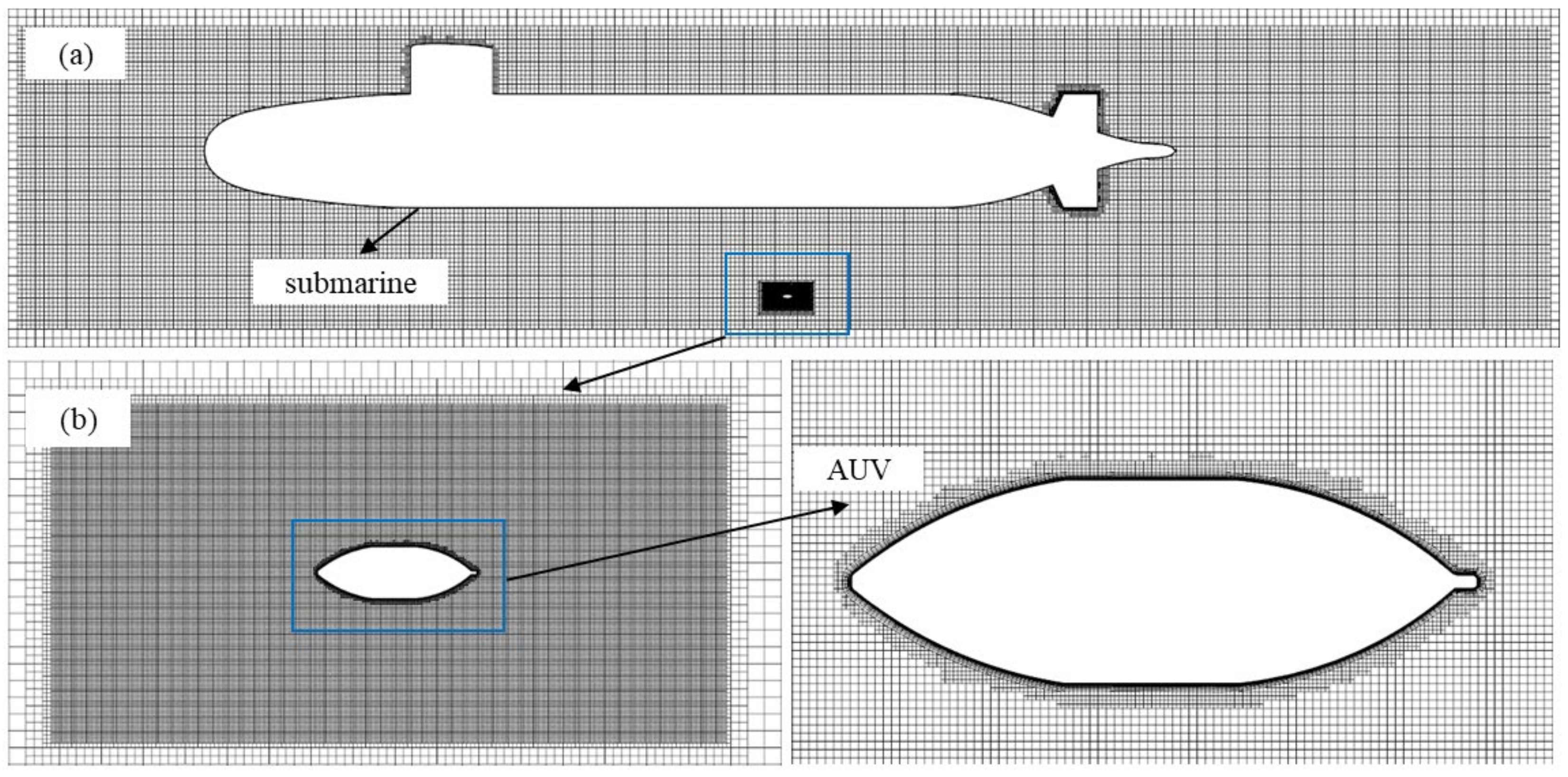
Figure 2 illustrates the schematic of the fluid domain used in our simulation, where the AUV is positioned directly beneath the submarine. As the AUV is much smaller than the submarine, we magnified it ten times for increased clarity. The length of the fluid domain is 5.0 L, with 1.0 L located before the submarine and 3.0 L behind it. The width and height of the fluid domain are both 1.0 L. Our simulation required a sufficiently large fluid domain to prevent any potential backflow from affecting the numerical results. The boundary conditions are shown in Figure 2.

The inlet boundary of the region is specified with a velocity inlet condition, while the outlet boundary is set with a pressure outlet condition. The bottom, side, and top boundaries are treated as velocity inlets, consistent with the velocity inlet boundary. The symmetry plane serves as a symmetric boundary condition. The submarine and AUV are treated as impermeable walls with a no-slip condition. For detailed boundary conditions, please refer to

Table 2. Boundary parameters.

Boundary	Boundary Parameter
Inlet	Velocity Inlet, flow speed = (Uo,0,0) m/s, turbulence intensity 0.01
Outlet	Pressure Outlet, hydrostatic pressure
Bottom/side/top	Same as inlet
Submarine	Impermeability wall with no-slip condition
AUV	Impermeability wall with no-slip condition
Symmetry plane	Symmetry plane

.

2.2.3. Meshing

In this study, to ensure accurate calculations of the flow field and resistance, the mesh set must be able to accurately depict the model’s shape, while also capturing the surrounding flow field and the force and vortex structure of the boundary layer of the hull. Mesh generation in this study was performed using the advanced automatic meshing capabilities of STAR-CCM+, which employs the highly efficient Cartesian cut-cell method. To accurately capture the boundary layer near the surfaces of the submarine and AUV, an orthogonal prism layer was generated. This layer consisted of prismatic cells that gradually increased in thickness by a constant scale factor of 1.1, ensuring proper resolution of the flow behavior. The first layer of the prism layer mesh was specifically placed within the logarithmic region of the boundary layer, targeting the range of 30 < Y+ < 100. This approach helped to accurately model the near-wall flow phenomena. In addition, the trimmer mesh, consisting mostly of hexahedral elements, discretized the majority of the computational domain. The trimmer mesh was chosen for its ability to efficiently represent the complex geometry of the simulation. The total number of meshes employed in the calculations amounted to 6,136,820. Around the AUV, the minimum grid step size was determined to be 0.018 m (L_AUV/242), whereas around the submarine, it was 0.4 m (L_submarine/217.8). Figure 3 shows the meshes of the computational domain, Submarine, and AUV.

3. Reliability of Numerical Models

Before applying any numerical method to carry out a simulation, it is essential to first verify its reliability. In this section, we present two typical experimental results to demonstrate the credibility of our numerical method. The first result involves the pressure distribution on the surface of the SUBOFF in a uniform incoming flow. We compared the simulated results against the corresponding experimental data and found that they were in good agreement, validating the accuracy of our numerical method. The second result involved a pair of similar ellipsoids in proximity at separation-length ratios.

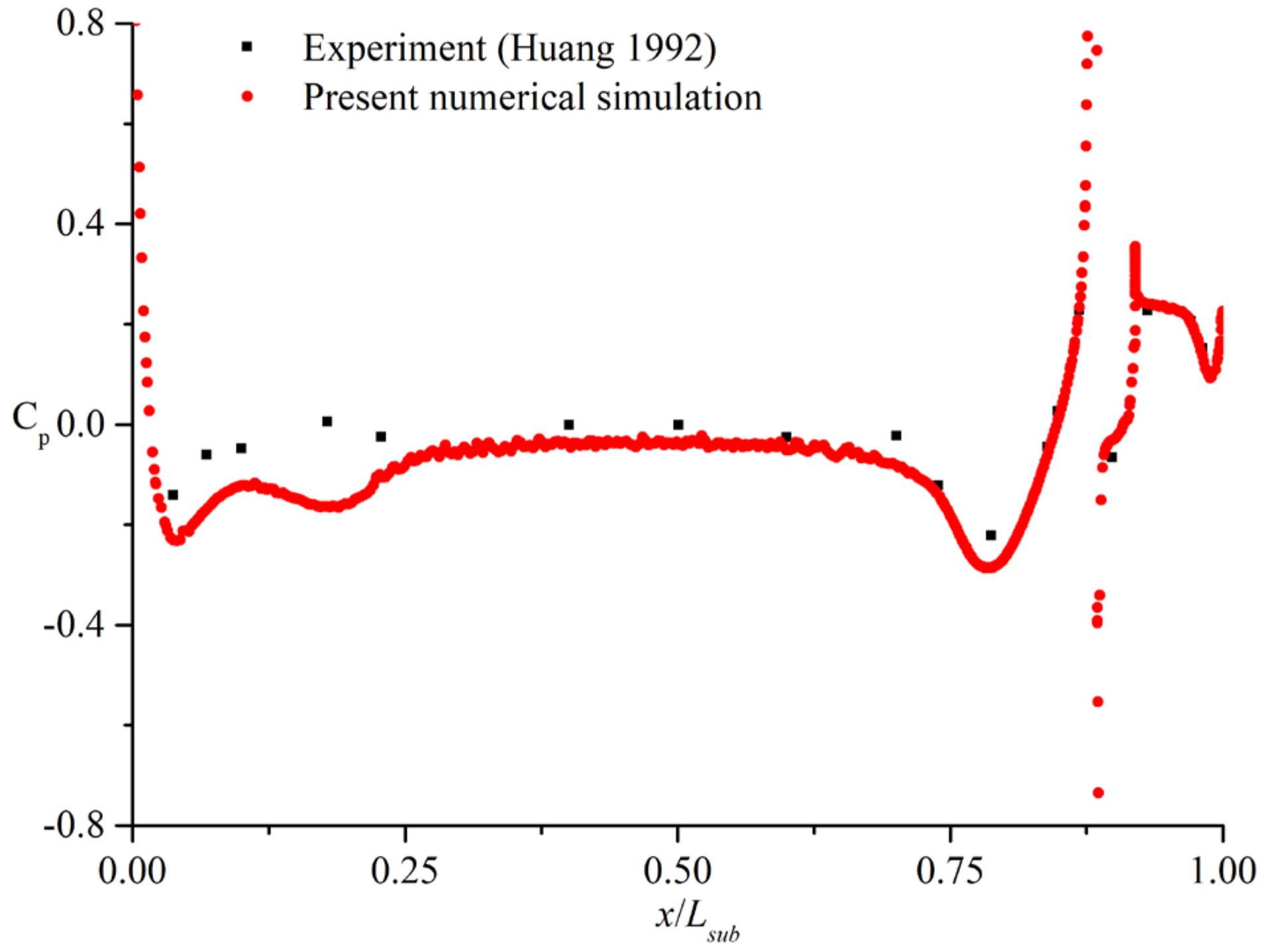
3.1. The Pressure Distribution on the Longitudinal Section and Resistance of the SUBOFF

To verify the mesh independence of our research, we utilized SUBOFF as the research object under the sailing condition of infinite depth with a speed of 5.144 m/s. We then adjusted the mesh base size and defined three distinct mesh sizes: coarse mesh, medium mesh, and fine mesh. The number of meshes under the same base size were 2.582 million, 3.846 million, and 6.823 million, respectively. Based on our calculations, the resistance values under these three mesh conditions were 275.6 N, 280.25 N, and 281.4 N, respectively. Notably, the experimental value is 283.8 N [41]. However, the errors between the calculated results and experimental values under various mesh conditions were all within 5%. Considering both calculation accuracy and efficiency, we determined that the medium mesh was the most suitable for our research. See

Table 3. Resistance results for different mesh numbers.

-	Coarse Mesh	Medium Mesh	Fine Mesh	Experimental Results
Mesh number (Million)	2.582	3.846	6.823	-
Resistance (N)	275.6	280.25	281.4	283.8
Error (%)	2.89	1.25	0.85	-

.

Huang et al. [42] have conducted a lot of work on the DARPA SUBOFF model under various Reynolds numbers, whether drag experiments or flow field measurements. Here, the pressure distributions on the SUBOFF AFF-8 surface when the Reynolds number is 1.2 × 10⁶ are used to verify the reliability of the numerical method. The dimensionless pressure coefficient is defined as

$${\mathrm{C}}_{\mathrm{p}}=\frac{P-P_{\infty }}{\rho U^2/2}$$

(6)

where P_∞ and U are the free-stream static pressure and uniform flow velocity in the velocity inlet, respectively. The C_p on the middle longitudinal section of the SUBOFF AFF-8 model obtained by the numerical simulation is compared with the experimental results [41]. The comparison between the numerical results and experimental results is shown in Figure 4. It can be seen that the results obtained from the numerical simulation have good agreement with the experiment results, which proves the reliability of the numerical methods used in this paper.

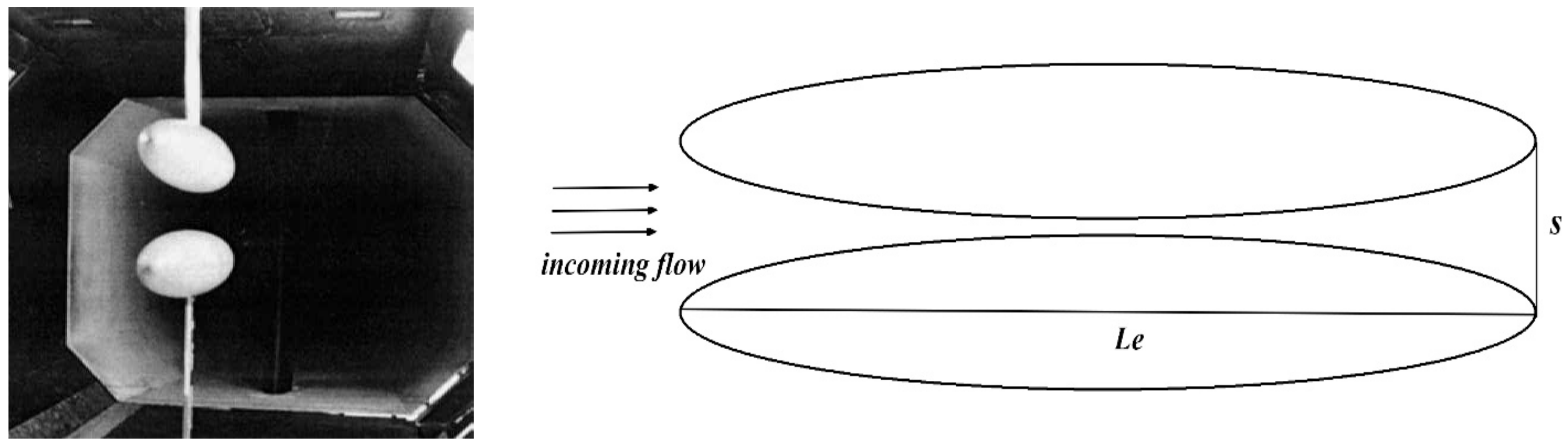
3.2. A Pair of Similar Ellipsoids in Proximity at Separation-Length Ratios

Molland [24,25] has conducted a lot of work on the hydrodynamic interaction between simple structures, such as the resistance change and pressure distribution when two ellipsoids are very close. The experimental photographs and 2D (two-dimensional) schematic of the two similar ellipsoids are shown in Figure 5. As shown in the figure, the model ellipsoids were constructed from glass-reinforced plastic (GRP). They have an overall length of 1200 mm, a maximum diameter of 200 mm, an eccentricity of 0, and a surface area of 0.601 m². The two ellipsoids are exactly the same, the ratio of their long and short axes is 6, and s is defined as the separation between the center lines of the two ellipsoids. Here, the pressure coefficient on the longitudinal section of the above ellipsoid is used to verify the numerical method, where the Reynolds number Is 3.2 × 10⁶ and s/L_e = 0.27 and 0.37.

The results of the numerical simulation and the experiment are shown in Figure 6. It can be seen that there is almost no difference between the two, which further proves the accuracy of the numerical method in this paper.

4. Results Analysis

This section aims to analyze the hydrodynamic interaction when the submarine and AUV remain relatively stationary. Two factors are considered in this analysis: the speed and position of the AUV relative to the submarine. The main focus is on the forces acting on the AUV, with additional important flow field information also presented. As the size of the submarine is significantly larger than that of the AUV, the hydrodynamic interaction has minimal effect on the submarine. Accordingly, this paper chooses to disregard the influence of the submarine on the simulation and analysis.

Figure 7 illustrates the relative position between the AUV and the submarine, with the AUV magnified ten times for better visualization, as was done in Figure 2. The AUV is positioned directly beneath the submarine, as shown. To accurately represent the position of the AUV relative to the submarine, we introduce two additional parameters: s and l. The length of the submarine (L) is 87.12 m, as previously defined. The parameter s represents the vertical distance between the center line of the submarine and the AUV. The parameter l represents the longitudinal distance from the geometric center of the AUV to the forefront of the submarine.

In the following simulation, the position of the AUV relative to the submarine will be dimensionless through the three parameters L, s, and l. In order to fully investigate the hydrodynamic interaction of the AUV at different positions, l/L is taken as 0, 0.1, 0.2, 0.4, 0.6, 0.8, 0.9, and 1.0. And, s/L is taken as 0.20, 0.15, 0.12, 0.10, 0.08, and 0.062. In addition, the influence of velocity has also been considered. The simulations are investigated with five speeds at each position, which are 2.0 kn (1.029 m/s), 3.0 kn (1.543 m/s), 4.0 kn (2.058 m/s), 5.0 kn (2.572 m/s), and 6.0 kn (3.087 m/s).

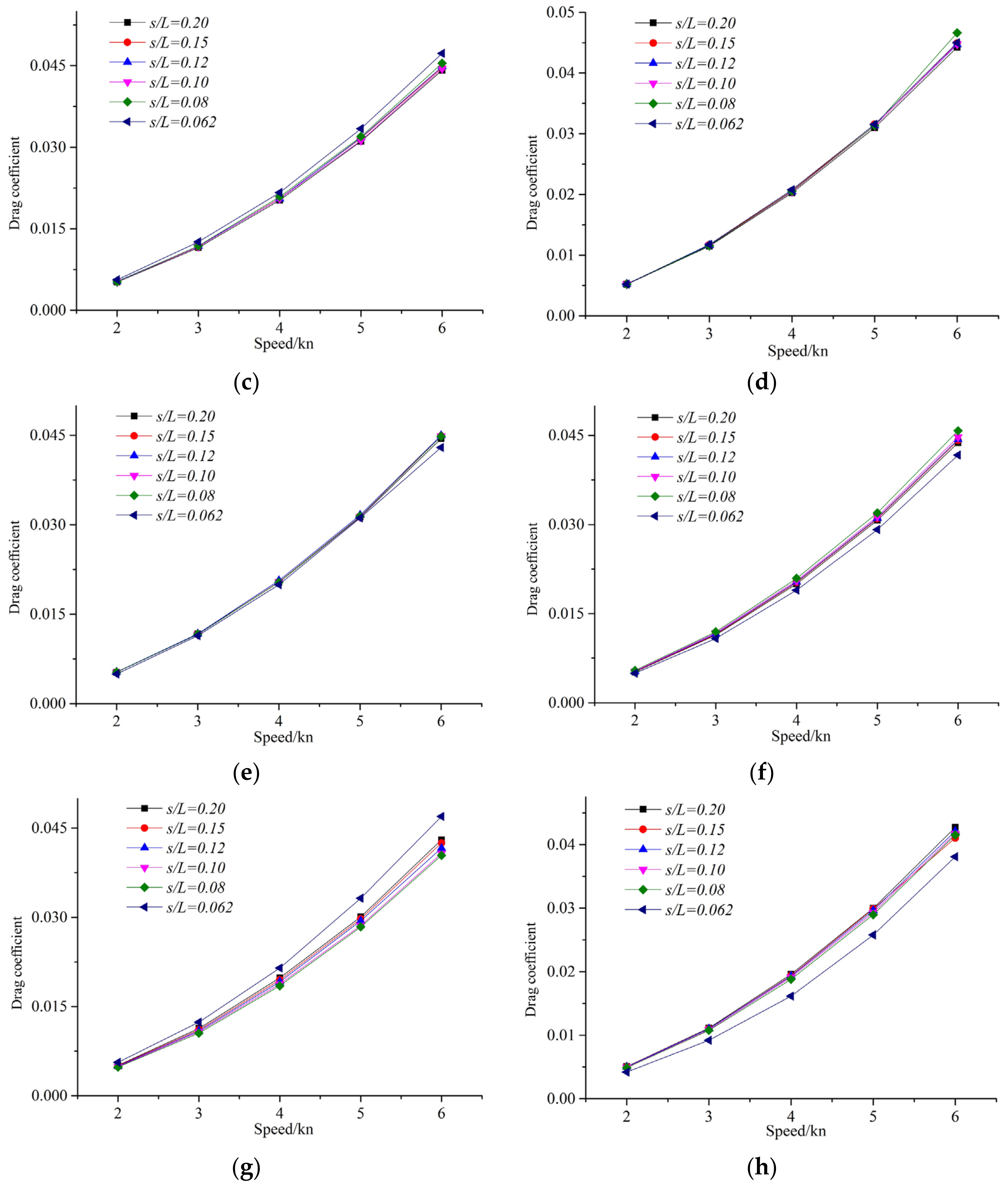
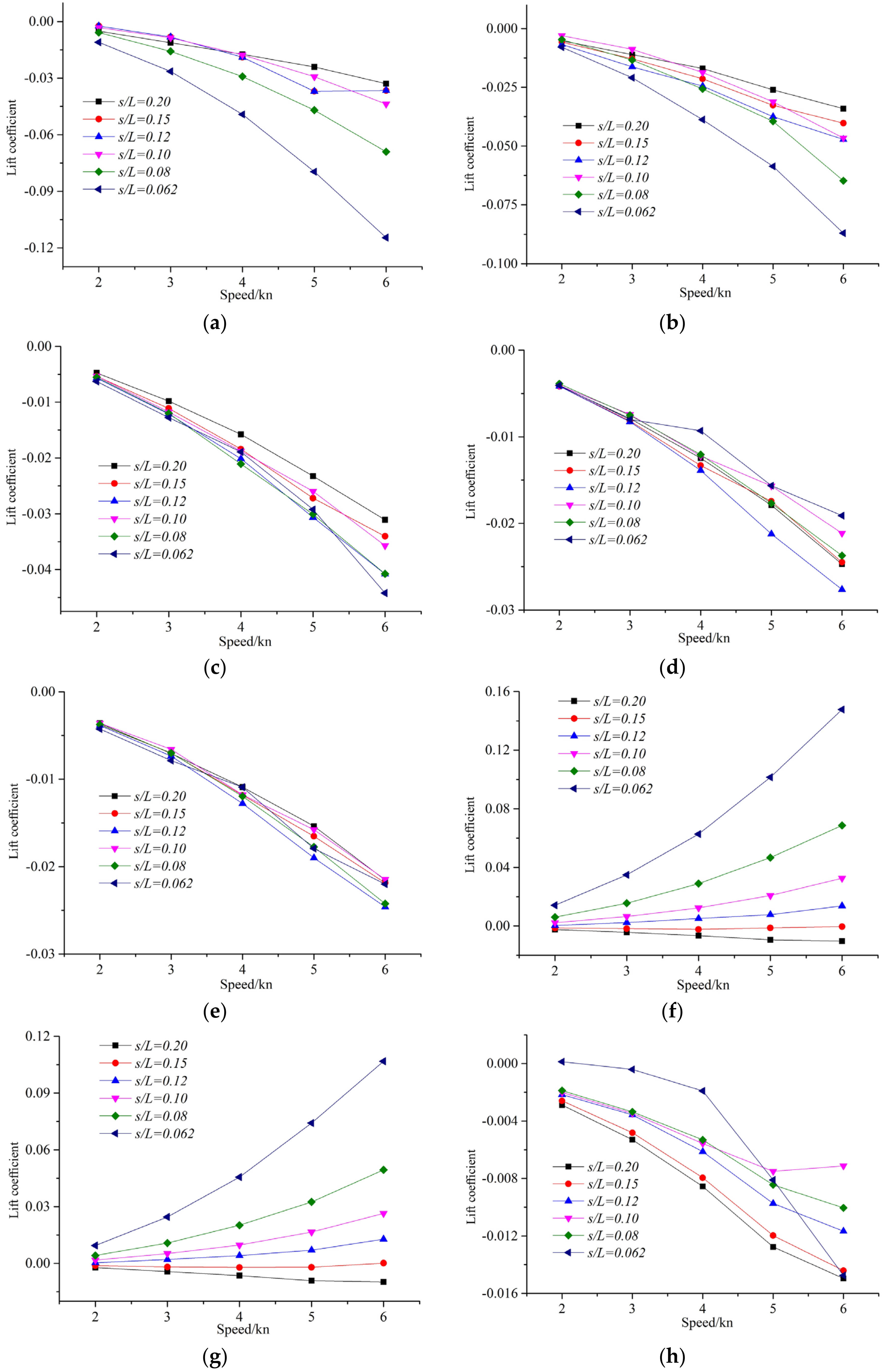
4.1. Results for Drag and Lift

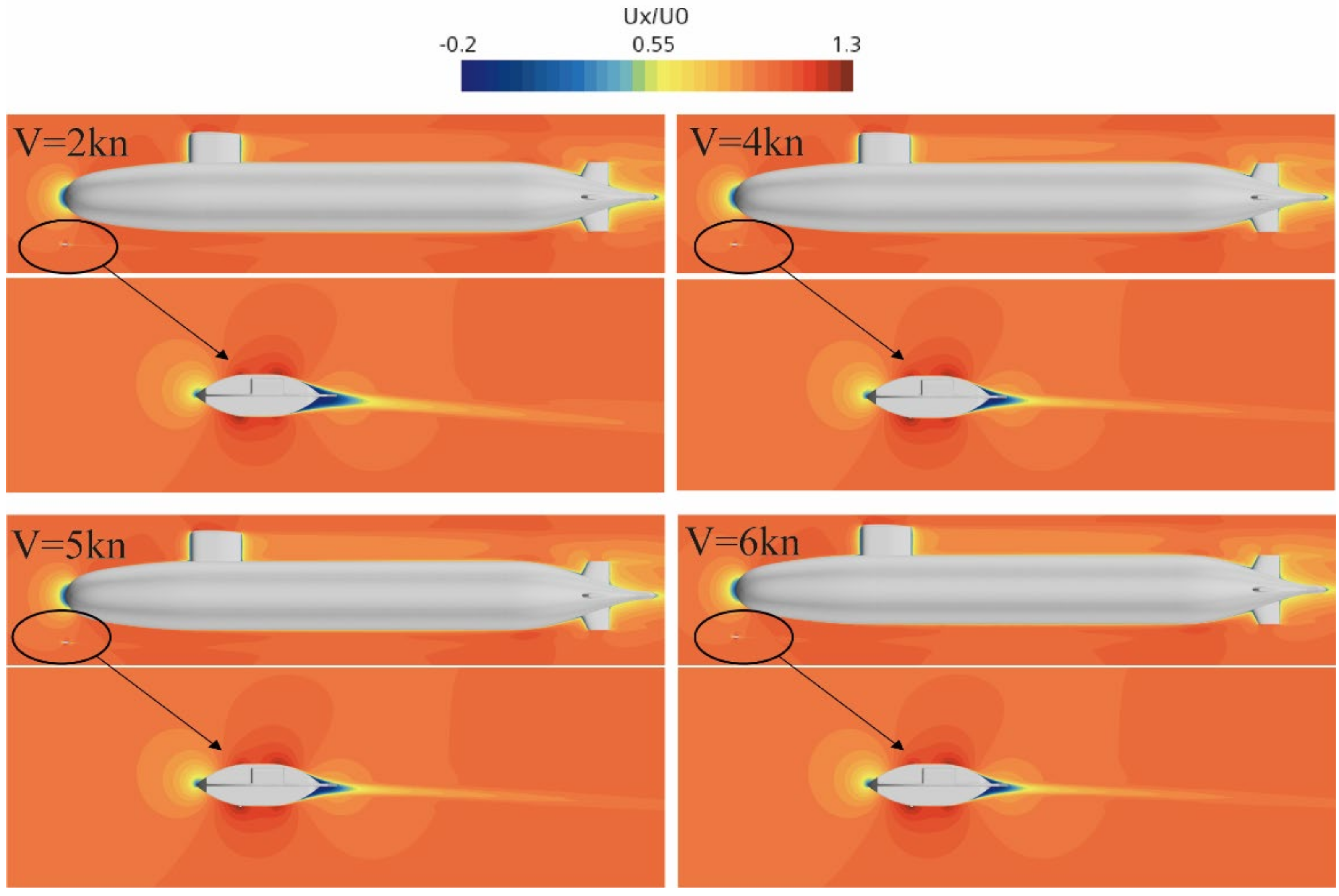
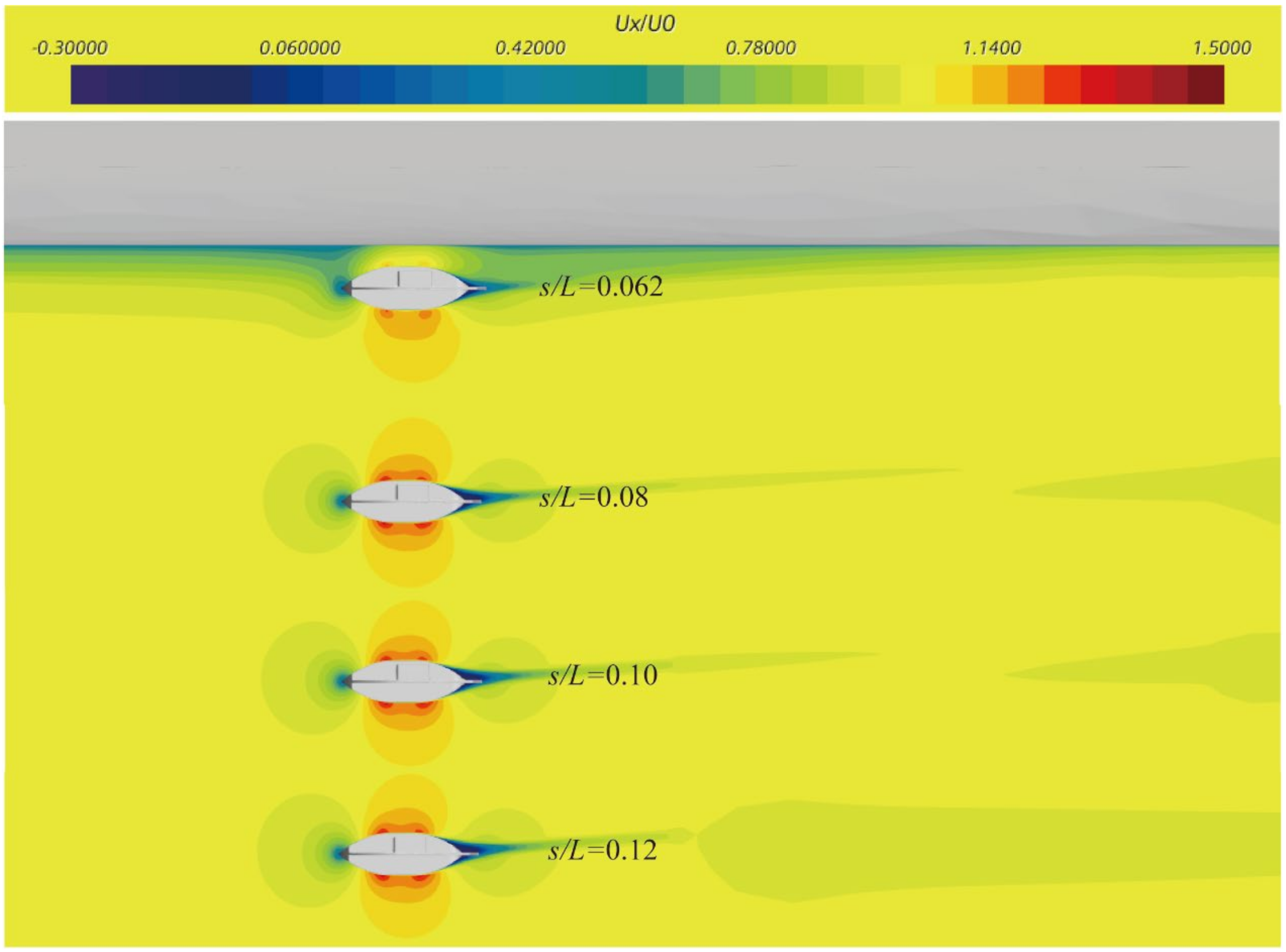
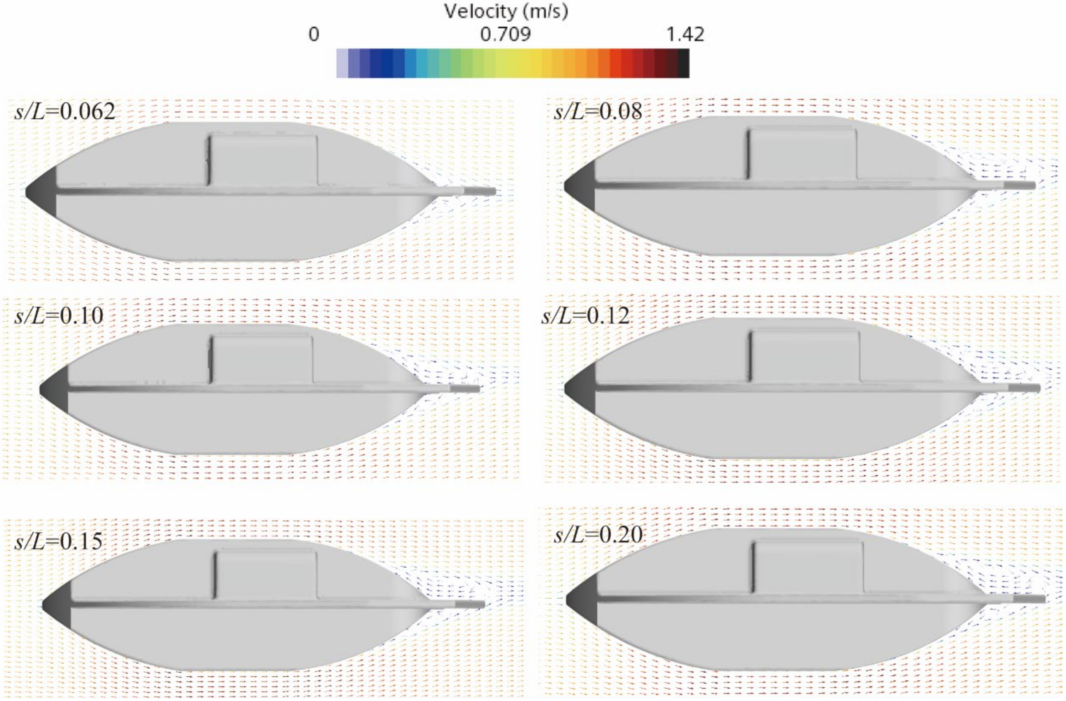
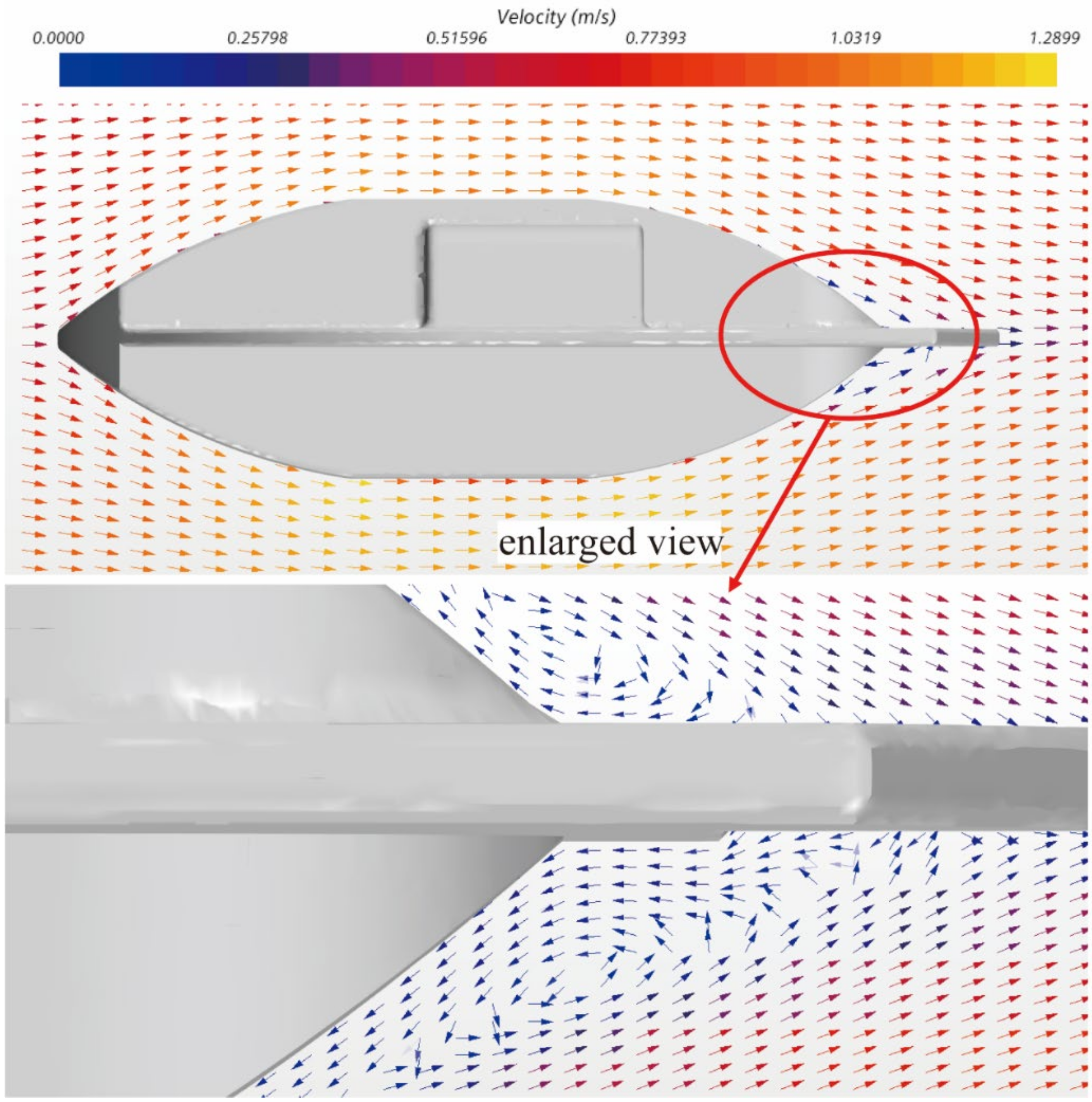
In this study, we selected eight longitudinal positions along the length of the submarine from bow to stern, which are denoted by l/L values of 0, 0.1, 0.2, 0.4, 0.6, 0.8, 0.9, and 1.0, respectively. Additionally, we selected six vertical positions from far to near, which are denoted by s/L values of 0.20, 0.15, 0.12, 0.10, 0.08, and 0.062. As a result, there are 48 positions of the AUV relative to the submarine that are considered in this analysis. The primary objective of this section is to examine the changes in the drag and lift of the AUV with respect to speed at these 48 positions and then compare the influence of the submarine on the AUV at different positions. All of the drag and lift values presented in this section are dimensionless by $0.5\rho U_{}^2{L}_a^2$; ρ is the density of water, which is 997.561 kg/m³. The length of the AUV (L_a) is 1.08 m, as shown in Table 1. Finally, U represents the speed of the AUV.

Figure 8 depicts the changes in drag with respect to speed at different vertical positions of the AUV relative to the submarine, while keeping the longitudinal position fixed. As evident from Figure 8a–h, the drag increases with an increase in speed. However, as the vertical distance between the AUV and the submarine decreases gradually, the drag does not change significantly. This observation suggests that when the AUV and the submarine are relatively stationary, the drag of the AUV is primarily influenced by its speed rather than the presence of the submarine. It is worth noting that when the AUV is positioned in the middle of the submarine, i.e., l/L values of 0.4, 0.6, and 0.8, the drag curves almost fully coincide. On the other hand, when the AUV is located towards the bow or stern of the submarine, the drag curves differ slightly. This difference can be attributed to the significant changes in the shape of the submarine towards its bow and stern resulting in a larger disturbance to the flow field. As the AUV moves closer to the submarine, this disturbance is stronger, thereby altering the drag. However, when the AUV is positioned in the middle of the submarine, where the geometric shape of the submarine remains relatively constant, the flow field is not disturbed, and the drag of the AUV remains nearly unchanged.

The lift, as shown in Figure 9, increases with an increase in speed, similar to drag. However, the lift also exhibits a dependence on the vertical distance between the AUV and the submarine, unlike drag. As the vertical distance decreases, the lift increases, with this trend becoming more apparent as the AUV moves closer to the submarine. Another crucial difference is that the lift properties differ significantly based on the position of the AUV relative to the submarine. When the AUV is located at longitudinal positions l/L = 0, 0.1, 0.2, 0.4, 0.6, and 1.0, the lift is negative, indicating repulsive hydrodynamic interaction between the AUV and the submarine. Moreover, when the AUV is closer to the submarine, the repulsive force becomes stronger. However, at l/L values of 0.8 and 0.9, if the AUV is positioned far away from the submarine, the lift remains negative. But, as the AUV approaches the submarine, the lift becomes positive, indicating attractive hydrodynamic interaction. This attractive force increases rapidly with the increase in speed as the AUV moves closer to the submarine.

Figure 10 presents a comparison of the drag of the AUV at various longitudinal positions relative to the submarine. It is noticeable that when the vertical distance between the AUV and the submarine is significant, i.e., s/L = 0.20, the hydrodynamic interaction has little impact on the drag of the AUV. Consequently, the drag remains practically constant at different longitudinal positions. However, as the AUV moves closer to the submarine, the differences in drag become more pronounced across various positions. It can be observed that the drag of the AUV is highest when it is located at the middle of the submarine, while the drag is lowest when it is located towards the bow. These results indicate that the shape of the submarine has a critical impact on the flow field around the AUV. The changes in the shape of the submarine towards its bow and stern result in a larger disturbance to the flow field, thereby modifying the drag coefficient. However, when the AUV is placed in the middle of the submarine, where the geometric shape of the vessel remains relatively constant, the flow field is not disturbed, resulting in higher drag values.

Figure 11 illustrates a comparison of the lift of the AUV at different longitudinal positions relative to the submarine. It is apparent that the AUV’s lift varies significantly, depending on its position in relation to the submarine. When the AUV is positioned towards the bow and middle of the submarine, i.e., l/L = 0, 0.1, 0.2, 0.4, and 0.6, the lift exhibits a similar trend. In these positions, the lift is always repulsive. Moreover, the magnitude of the lift at the bow of the submarine is larger than that at the middle for the same speed. This indicates that the geometry of the submarine has a critical impact on the lift properties of the AUV. The flow field around the AUV is more disturbed by the presence of the submarine towards its bow than in the middle region, resulting in higher lift values.

When the AUV is positioned towards the stern of the submarine, the situation is different. For l/L = 0.8 and 0.9, the lift exhibits a similar trend, where an increase in speed results in a rapid increase in lift. Additionally, when the AUV is far from the submarine, the lift force is repulsive, while the lift force becomes attractive when the AUV is close to the submarine. However, it can be observed that the lift is always a repulsive force for l/L = 1.0. It is worth noting that the impact of speed on lift is relatively small, and the increase in lift with speed is negligible. Furthermore, the influence of speed decreases as the AUV moves closer to the submarine. These observations highlight the complexity of the flow field around the AUV and submarine system. The intricate geometrical features of the submarine result in an intricate flow pattern, affecting the lift characteristics of the AUV.

4.2. Velocity Field

4.2.1. l/L = 0, s/L = 0.08

In this study, the AUV is much smaller than the submarine, making it more susceptible to flow disruption. Therefore, only the influence of the AUV’s velocity field is analyzed in this section. The distribution of AUV’s velocity field under different conditions is analyzed. Figure 12 illustrates the velocity field distribution when the vertical distance between the AUV and submarine is l/L = 0 and the longitudinal distance s/L = 0.08, with speeds of 2 kn, 4 kn, 5 kn, and 6 kn. The X-axis speed U_x is dimensionless and denoted as U_x/U₀, where U₀ represents the initial sailing speed. The AUV navigates in the flow field of the submarine’s bow area, where the surrounding flow field is disturbed by the submarine. Due to the suction effect created by the submarine, the velocity field on the upper surface of the AUV exhibits asymmetric distribution, while the lower surface is less disturbed, showing a relatively symmetrical velocity field distribution. Low-speed areas appear in the bow and stern regions of the AUV, with high-speed areas present on both the upper and lower surfaces. At different speeds, the low-speed recirculation zone at the stern of the AUV slightly decreases with an increase in speed.

Figure 13 and Figure 14 present the velocity field distribution at different speeds for l/L = 0.6, s/L = 0.062 and l/L = 1.0, s/L = 0.08, respectively. As shown in Figure 13, when the AUV is sailing in the middle of the submarine, the flow field on the upper surface is significantly disrupted by the presence of the submarine. Moreover, as the speed increases, the high-speed flow field area increases. On the other hand, the lower surface of the AUV exhibits relatively low disturbance, showing a relatively symmetrical velocity field distribution. In Figure 14, the AUV is sailing at the stern of the submarine. Here, due to the relatively far position from the wake area of the submarine, the influence on the AUV’s flow field at different speeds is minimal, with negligible changes in the velocity field distribution observed.

4.2.2. s/L = 0.08, V = 2 kn

This study analyzes the velocity field distribution at different longitudinal distances. Specifically, the longitudinal distance between the submarine and AUV is set at s/L = 0.08, while the speed is 2 kn. Figure 15 shows the longitudinal position diagram of the AUV. As the AUV is much smaller than the submarine, an enlarged view of the velocity field distribution is presented in Figure 16 to provide a clearer visualization of the flow field.

The velocity field surrounding the AUV is significantly influenced by the presence of the submarine, causing disturbances in the flow field. The distribution of velocity fields under different conditions reveals that low-speed reflux zones appear at the bow and stern regions of the AUV, with high-speed zones appearing on both the upper and lower surfaces. The velocity field distribution on the upper surface of the AUV appears asymmetric when l/L = 0, 0.1, and 0.2, while the distribution on the lower surface is relatively symmetrical. In contrast, the velocity field distribution on both the upper and lower surfaces of the AUV is symmetric when l/L = 0.4 and 0.6. At l/L = 0.8, the velocity field distribution on the upper surface of the AUV is symmetrical, while it becomes asymmetric on the lower surface. In addition, when the AUV approaches the stern area of the submarine (l/L = 0.9), the low-speed areas on both the upper and lower surfaces increase due to the interference of the stern rudder. When l/L = 1.0, since the AUV is further away from the submarine, it is less affected, and the distribution of velocity fields on both the upper and lower surfaces is basically symmetrical.

4.2.3. l/L = 0.6, V = 2 kn

In this study, the velocity field distribution at different vertical distances has been analyzed. To provide a clearer visualization of the flow patterns under different conditions, Figure 17 presents an enlarged view of the velocity field distribution at different vertical positions. As shown in Figure 16, all conditions have been presented in one diagram for ease of comparison. When s/L = 0.062, it can be observed that the flow field on the upper surface and bow and stern areas of the AUV is significantly disturbed due to the adsorption effect of the submarine, resulting in a low-speed zone. This effect is caused by the submarine’s interference with the surrounding water flow, leading to an uneven velocity field distribution. However, when the longitudinal distance between the submarine and AUV is further increased to s/L = 0.08, 0.10, and 0.12, the AUV is far away from the submarine, and the influence of the submarine on the surrounding flow field is negligible. Consequently, the flow field surrounding the AUV is basically unaffected by the presence of the submarine, resulting in a more stable velocity field distribution.

Figure 18 depicts the velocity vectors of the AUV at different vertical positions when l/L = 0.6 and V = 2 kn. The analysis indicates that when s/L = 0.062, the adsorption effect of the submarine causes the low-speed reflux area at the stern of the AUV to be smaller compared to other conditions. Conversely, when s/L = 0.08, 0.10, 0.12, 0.15, and 0.20, the AUV is less affected by the submarine, leading to a relatively large low-speed reflux zone. To visualize the vortex structure of the velocity vector affected by the submarine more clearly, Figure 19 presents an enlarged view of the aft region of the AUV under the s/L = 0.062 condition. As shown in Figure 18, a reflux zone appears at the stern area of the AUV, accompanied by the formation of vortex structures. This observation further confirms the effect of the submarine’s presence on the flow field surrounding the AUV.

4.3. Pressure s/L = 0.08, V = 2 kn

Figure 20 illustrates the pressure distribution of the AUV under different vertical distances, with s/L = 0.08 and V = 2 kn. Observations indicate that the high-pressure region of the AUV primarily appears in the bow area and the shape transition region of the upper surface. The AUV is significantly disrupted when it enters the bow flow field area of the submarine. Therefore, as l/L increases from 0 to 0.8, the AUV gradually moves away from the bow area, and the range of the high-pressure area gradually decreases. Furthermore, at l/L = 0.9 and 1.0, the high-pressure range increases near the stern rudder area due to the interference of the submarine’s stern rudder. The AUV experiences increasing pressure levels in this area, which can affect its overall stability and maneuverability.

5. Conclusions

The research background of this paper is based on the interference of the AUV by the mother ship during the recycling process. The AUV remains relatively stationary with the mother ship during the recovery process. The AUV sails at different vertical positions and longitudinal positions relative to the mother ship. And, the optimal position for the AUV to be least affected by the mother ship during the recovery process was obtained. The details are as follows:

(1)

When the vertical distance between the AUV and submarine changes, the resistance has little change, but when the speed changes, the resistance changes significantly.

(2)

When approaching the bow and stern area of the submarine, the AUV is more susceptible to interference, while in the parallel middle section, it is less susceptible to interference because the shape of the bow and stern of the submarine changes greatly, and the flow field disturbance is obvious.

(3)

The lift increases as the vertical distance between the AUV and the submarine decreases, and the closer it approaches the submarine, the more significant the change in lift. And, when the AUV is in different longitudinal positions on the submarine, when the lift is negative, there is a repulsive effect between the submarine and the AUV. When the lift is positive, the submarine exhibits an upward suction effect on the AUV.

(4)

The velocity and pressure fields of the AUV are affected by the submarine when sailing at different positions. At the mid-longitudinal position of the submarine, the impact is minimal, and it is the best position for recovery.

(5)

This paper focuses on the interference effects of the AUV and submarine when they remain relatively stationary. Further research is needed to investigate the interference effects of oblique motion recovery and non-relative static recovery.

In conclusion, the AUV moving through the water generates a resistance force due to the viscosity of the fluid. The submarine must, therefore, accelerate slowly during the recovery process. The movement of the submarine can cause disturbances in the surrounding fluid flow field. These disturbances may affect the motion of the AUV, causing it to move erratically or become unstable. Therefore, careful consideration must be given to the position and motion of the submarine during the recovery process.

References

1. Nicholson, J.W.; Healey, A.J. The present state of autonomous underwater vehicle (AUV) applications and technologies. Mar. Technol. Soc. J. 2008, 42, 44–51. [Google Scholar] [CrossRef]
2. Wang, H.J.; Long, X.; Li, J.; Zhou, H.N. Design, construction of a small unmanned underwater vehicle. In Proceedings of the 2013 MTS/IEEE OCEANS-Bergen, Bergen, Norway, 10–14 June 2013; pp. 1–6. [Google Scholar]
3. Nouri, N.M.; Zeinali, M.; Jahangardy, Y. AUV hull shape design based on desired pressure distribution. J. Mar. Sci. Technol. 2016, 21, 203–215. [Google Scholar] [CrossRef]
4. Yan, K.; Wu, L. A survey on the key technologies for underwater AUV docking. Robot 2007, 29, 267–273. [Google Scholar]
5. Zhang, W.; Wu, W.; Teng, Y.; Li, Z.; Yan, Z. An underwater docking system based on UUV and recovery mother ship: Design and experiment. Ocean Eng. 2023, 281, 114767. [Google Scholar] [CrossRef]
6. Szczotka, M. AUV launch & recovery handling simulation on a rough sea. Ocean Eng. 2022, 246, 110509. [Google Scholar]
7. Fan, S.; Liu, C.; Li, B.; Xu, Y.; Xu, W. UUV docking based on USBL navigation and vision guidance. J. Mar. Sci. Technol. 2019, 24, 673–685. [Google Scholar] [CrossRef]
8. Page, B.R.; Mahmoudian, N. Simulation-driven optimization of underwater docking station design. IEEE J. Ocean. Eng. 2019, 45, 404–413. [Google Scholar] [CrossRef]
9. Zhang, W.; Jia, G.; Wu, P.; Yang, S.; Huang, B.; Wu, D. Study on hydrodynamic characteristics of AUV launch process from a launch tube. Ocean Eng. 2021, 232, 109171. [Google Scholar] [CrossRef]
10. Brizzolara, S.; Chryssostomidis, C. Design of an Unconventional ASV for Underwater Vehicles Recovery: Simulation of the motions for operations in rough seas. In Proceedings of the ASNE International Conference on Launch and Recovery, Linthicum, MD, USA, 14–15 November 2012. [Google Scholar]
11. Sarda, E.I. Automated Launch and Recovery of an Autonomous Underwater Vehicle from an Unmanned Surface Vessel; Florida Atlantic University: Boca Raton, FL, USA, 2016. [Google Scholar]
12. Bai, G.; Gu, H.; Zhang, H.; Meng, L.; Tang, D. V-shaped wing design and hydrodynamic analysis based on moving base for recovery AUV. In Proceedings of the 2018 WRC Symposium on Advanced Robotics and Automation (WRC SARA), Beijing, China, 16 August 2018; pp. 320–325. [Google Scholar]
13. Palomeras, N.; Vallicrosa, G.; Mallios, A.; Bosch, J.; Vidal, E.; Hurtos, N.; Carreras, M.; Ridao, P. AUV homing and docking for remote operations. Ocean Eng. 2018, 154, 106–120. [Google Scholar] [CrossRef]
14. Meng, L.; Lin, Y.; Gu, H.; Bai, G.; Su, T.C. Study on dynamic characteristics analysis of underwater dynamic docking device. Ocean Eng. 2019, 180, 1–9. [Google Scholar] [CrossRef]
15. Li, Y.; Jiang, Y.; Cao, J.; Wang, B.; Li, Y. AUV docking experiments based on vision positioning using two cameras. Ocean Eng. 2015, 110, 163–173. [Google Scholar] [CrossRef]
16. Lin, M.; Yang, C. Auv docking method in a confined reservoir with good visibility. J. Intell. Robot. Syst. 2020, 100, 349–361. [Google Scholar] [CrossRef]
17. Vu, M.T.; Choi, H.S.; Nhat, T.Q.M.; Nguyen, N.D.; Lee, S.D.; Le, T.H.; Sur, J. Docking assessment algorithm for autonomous underwater vehicles. Appl. Ocean Res. 2020, 100, 102180. [Google Scholar] [CrossRef]
18. Hardy, T.; Barlow, G. Unmanned Underwater Vehicle (UUV) deployment and retrieval considerations for submarines. In Proceedings of the International Naval Engineering Conference and Exhibition 2008, Hamburg, Germany, 13 April 2008. [Google Scholar]
19. Mawby, A.; Wilson, P.; Bole, M.; Fiddes, S.P.; Duncan, J. Manoeuvring Simulation of Multiple Underwater Vehicles in Close Proximity; SEA (Group) Ltd.: Frome, UK, 2010. [Google Scholar]
20. Kim, J.; Lee, G. A study on the UUV docking system by using torpedo tubes. In Proceedings of the 2011 8th International Conference on Ubiquitous Robots and Ambient Intelligence (URAI), Incheon, Republic of Korea, 23–26 November 2011; pp. 842–844. [Google Scholar]
21. Meng, L.; Lin, Y.; Gu, H.; Su, T.C. Study on dynamic docking process and collision problems of captured-rod docking method. Ocean Eng. 2019, 193, 106624. [Google Scholar] [CrossRef]
22. Yang, Q.; Liu, H.; Yu, X.; Zhang, W.; Chen, J. Attitude constraint-based recovery for under-actuated AUVs under vertical plane control during the capture stage. Ocean Eng. 2023, 281, 115012. [Google Scholar] [CrossRef]
23. Molland, A.F.; Utama, I.K.A.P. Wind Tunnel Investigation of a Pair of Ellipsoids in Close Proximity; University of Southampton: Southampton, UK, 1997. [Google Scholar]
24. Molland, A.F.; Utama, I.K.A.P. Experimental and numerical investigations into the drag characteristics of a pair of ellipsoids in close proximity. Proc. Inst. Mech. Eng. Part M J. Eng. Marit. Environ. 2002, 216, 107–115. [Google Scholar] [CrossRef]
25. Husaini, M.; Samad, Z.; Arshad, M.R. CFD simulation of cooperative AUV motion. Indian J. Mar. Sci. 2009, 38, 346–351. [Google Scholar]
26. Zhang, D.; Chao, L.; Pan, G. Analysis of hydrodynamic interaction impacts on a two-AUV system. Sh. Offshore Struct. 2019, 14, 23–34. [Google Scholar] [CrossRef]
27. Rattanasiri, P.; Wilson, P.A.; Phillips, A.B. Numerical investigation of a fleet of towed AUVs. Ocean Eng. 2014, 80, 25–35. [Google Scholar] [CrossRef]
28. Mitra, A.; Panda, J.P.; Warrior, H.V. Experimental and numerical investigation of the hydrodynamic characteristics of Autonomous Underwater Vehicles over sea-beds with complex topography. Ocean Eng. 2020, 198, 106978. [Google Scholar] [CrossRef]
29. Zhang, W.; Zeng, J.; Yan, Z.; Wei, S.; Tian, W. Leader-following consensus of discrete-time multi-AUV recovery system with time-varying delay. Ocean Eng. 2021, 219, 108258. [Google Scholar] [CrossRef]
30. Wu, L.; Li, Y.; Su, S.; Yan, P.; Qin, Y. Hydrodynamic analysis of AUV underwater docking with a cone-shaped dock under ocean currents. Ocean Eng. 2014, 85, 110–126. [Google Scholar] [CrossRef]
31. Meng, L.; Lin, Y.; Gu, H.; Su, T.C. Study on the mechanics characteristics of an underwater towing system for recycling an Autonomous Underwater Vehicle (AUV). Appl. Ocean Res. 2018, 79, 123–133. [Google Scholar] [CrossRef]
32. Meng, L.S.; Lin, Y.; Gu, H.T.; Su, T.C. Study of the Dynamic Characteristics of a Cone-Shaped Recovery System on Submarines for Recovering Autonomous Underwater Vehicle. China Ocean Eng. 2020, 34, 387–399. [Google Scholar] [CrossRef]
33. Fedor, R. Simulation of a Launch and Recovery of an UUV to an Submarine; KTH Royal Institute of Technology: Stockholm, Sweden, 2009. [Google Scholar]
34. Leong, Z.Q.; Saad, K.; Ranmuthugala, S.D.; Duffy, J.T. Investigation into the hydrodynamic interaction effects on an AUV operating close to a submarine. In Proceedings of the Pacific 2013 International Maritime Conference, Sydney, Australia, 7–9 October 2013; pp. 1–11. [Google Scholar]
35. Leong, Z.Q.; Ranmuthugala, D.; Penesis, I.; Nguyen, H. Quasi-static analysis of the hydrodynamic interaction effects on an autonomous underwater vehicle operating in proximity to a moving submarine. Ocean Eng. 2015, 106, 175–188. [Google Scholar] [CrossRef]
36. Leong, Z.Q.; Ranmuthugala, D.; Forrest, A.L.; Duffy, J. Numerical investigation of the hydrodynamic interaction between two underwater bodies in relative motion. Appl. Ocean Res. 2015, 51, 14–24. [Google Scholar]
37. Du, X.; Zheng, Z.; Guan, S. Numerical Calculation of Hydrodynamic Interactions of Submarine Flow on AUV. In Proceedings of the OCEANS-MTS/IEEE Kobe Techno-Oceans (OTO), Kobe, Japan, 28–31 May 2018; pp. 1–5. [Google Scholar]
38. Groves, N.C.; Huang, T.T.; Chang, M.S. Geometric Characteristics of DARPA SUBOFF Models (DTRC Model Nos 5470 and 5471); David Taylor Research Center: Bethesda, MD, USA, 1989. [Google Scholar]
39. Menter, F.R. Two-equation eddy-viscosity turbulence models for engineering applications. AIAA J. 1994, 32, 1598–1605. [Google Scholar] [CrossRef]
40. Larsson, L.; Raven, H. Ship Resistance and Flow; Society of Naval Architects and Marine Engineering: New York, NY, USA, 2010. [Google Scholar]
41. Liu, H.; Huang, T.T. Summary of DARPA SUBOFF Experimental Program Data; Naval Surface Warfare Center Carderock Div: Bethesda, MD, USA, 1998. [Google Scholar]
42. Huang, T.; Liu, H.L.; Groves, N.; Forlini, T.; Blanton, J.; Gowing, S. Measurements of flows over an axisymmetric body with various appendages in a wind tunnel: The DARPA SUBOFF experimental program. In Proceedings of the 19th Symposium on Naval Hydrodynamics, Seoul, Republic of Korea, 23–28 August 1992; pp. 312–346. [Google Scholar]
Figure 1. Schematic of simulation mode; (a) SUBOFF AFF-8; (b) AUV (Top view); (c) AUV (Side view).
Jmse 11 01789 g001
Figure 2. Schematic of fluid domain.
Jmse 11 01789 g002
Figure 3. Mesh refinement of the computational domain; (a) Overall meshes; (b) Local mesh refinement of the AUV.
Jmse 11 01789 g003
Figure 4. Pressure coefficients on the middle longitudinal section of the SUBOFF AFF-8 model [42].
Jmse 11 01789 g004
Figure 5. The experimental photographs (left) and 2D schematic (right) of a pair of ellipsoids in proximity.
Jmse 11 01789 g005
Figure 6. The pressure coefficient on the longitudinal section of the above ellipsoid: (a) s/Le = 0.27, (b) s/Le = 0.37 [23].
Jmse 11 01789 g006
Figure 7. The schematic of the relative position of the AUV and submarine.
Jmse 11 01789 g007
Figure 8. The dimensionless drag of the AUV in different vertical positions: (a) l/L = 0, (b) l/L = 0.1, (c) l/L = 0.2, (d) l/L = 0.4, (e) l/L = 0.6, (f) l/L = 0.8, (g) l/L = 0.9, (h) l/L = 1.0.
Jmse 11 01789 g008aJmse 11 01789 g008b
Figure 9. The dimensionless lift of the AUV in different vertical positions: (a) l/L = 0, (b) l/L = 0.1, (c) l/L = 0.2, (d) l/L = 0.4, (e) l/L = 0.6, (f) l/L = 0.8, (g) l/L = 0.9, (h) l/L = 1.0.
Jmse 11 01789 g009
Figure 10. The dimensionless drag of the AUV in different longitudinal positions: (a) s/L = 0.2, (b) s/L = 0.15, (c) s/L = 0.12, (d) s/L = 0.10, (e) s/L = 0.08, (f) s/L = 0.062.
Jmse 11 01789 g010
Figure 11. The dimensionless lift of the AUV in different longitudinal positions: (a) s/L = 0.2, (b) s/L = 0.15, (c) s/L = 0.12, (d) s/L = 0.10, (e) s/L = 0.08, (f) s/L = 0.062.
Jmse 11 01789 g011
Figure 12. Velocity field distribution with different speeds at l/L = 0, s/L = 0.08.
Jmse 11 01789 g012
Figure 13. Velocity field distribution with different speeds at l/L = 0.6, s/L = 0.062.
Jmse 11 01789 g013
Figure 14. Velocity field distribution with different speeds at l/L = 1.0, s/L = 0.08.
Jmse 11 01789 g014
Figure 15. Longitudinal position diagram of the AUV.
Jmse 11 01789 g015
Figure 16. Enlarged view of velocity field distribution at different longitudinal positions.
Jmse 11 01789 g016
Figure 17. Enlarged view of velocity field distribution at different vertical positions.
Jmse 11 01789 g017
Figure 18. Velocity vectors of AUV at different vertical positions.
Jmse 11 01789 g018
Figure 19. Enlarged view of velocity vectors of AUV at l/L = 0.6, s/L = 0.062, and V = 2 kn.
Jmse 11 01789 g019
Figure 20. Pressure distribution.
Jmse 11 01789 g020