
A Package of Script Codes, POSIBIOM for Vegetation Acoustics: POSIdonia BIOMass

Faculty of Fisheries, Main Campus, Akdeniz University, 07050 Antalya, Turkey
J. Mar. Sci. Eng. 2023, 11(9), 1790; https://doi.org/10.3390/jmse11091790
Submission received: 16 August 2023
/
Revised: 9 September 2023
/
Accepted: 12 September 2023
/
Published: 13 September 2023
(This article belongs to the Special Issue Advanced Remote Sensing Engineering Applied in the Environmental Monitoring of the Coasts)
Abstract
:Macrophytes and seagrasses play a crucial role in a variety of functions in marine ecosystems and respond in a synchronized manner to a changing climate and the subsequent ecological status. The monitoring of seagrasses is one of the most important issues in the marine environment. One rapidly emerging monitoring technique is the use of acoustics, which has advantages compared to other remote sensing techniques. The acoustic method alone is ambiguous regarding the identities of backscatterers. Therefore, a computer program package was developed to identify and estimate the leaf biometrics (leaf length and biomass) of one of the most common seagrasses, Posidonia oceanica. Some problems in the acoustic data were resolved in order to obtain estimates related to problems with vegetation as well as fisheries and plankton acoustics. One of the problems was the “lost” bottom that occurred during the data collection and postprocessing due to the presence of acoustic noise, reverberation, interferences and intense scatterers, such as fish shoals. Another problem to be eliminated was the occurrence of near-bottom echoes belonging to submerged vegetation, such as seagrasses, followed by spurious echoes during the survey. The last one was the recognition of the seagrass to estimate the leaf length and biomass, the calibration of the sheaths/vertical rhizomes of the seagrass and the establishment of relationships between the acoustic units and biometrics. As a result, an autonomous package of code written in MATLAB was developed to perform all the processes, named “POSIBIOM”, an acronym for POSIdonia BIOMass. This study presents the algorithms, methodology, acoustic–biometric relationship and mapping of biometrics for the first time, and discusses the advantages and disadvantages of the package compared to the software dedicated to the bottom types, habitat and vegetation acoustics. Future studies are recommended to improve the package.
1. Introduction
Aquatic macrophytes (algae, grasses, etc.) are an important component that plays a crucial role in various ways in aquatic ecosystems [1,2,3]. Considering the volume and surface area of marine systems, algae and seagrasses provide significant contributions, primarily consisting of oxygen production and carbon absorption/emission as part of the ocean–atmosphere interactions. Besides microscopic algae and photosynthetic bacteria, most marine macrophytes can reveal the level of a marine ecosystem’s health and ecological status. Some of them are indicators of pollution, while others are indicators of a pristine environment [4,5]. Unlike algae, seagrasses are associated with sediments (benthic system) by their below-ground parts (rhizomes and roots) [6] and with the pelagic system by their above-ground parts (sheaths and leaves) [5].
One of the most common seagrasses is Posidonia, a phanerogam species that occurs in nutrient-poor marine environments, where it can form abundant stands. Posidonia is a coastal species that is distributed worldwide in subtropical and temperate waters from Indo-Pacific Ocean (Australia) to Atlantic Ocean (Mediterranean Sea) systems [7,8]. Posidonia is highly sensitive to pollution, climate change, global warming, biogeochemical cycling, anthropogenic impacts, water movements, etc. [9,10,11]. Its biometric characteristics respond rapidly to global or local events, allowing scientists to monitor the health of marine systems. Like other seagrasses, Posidonia species can provide many useful habitats for other organisms under its canopies [4,12,13,14,15]. One of the most common Posidonia species is Posidonia oceanica (Linnaeus) Delile, 1813, which is an endemic species found in the Mediterranean Sea and extending to the near shore of the eastern Atlantic Ocean [16]. Most (25–30%) Mediterranean coasts are inhabited by P. oceanica [6].
Like other seagrasses (angiosperms), Posidonia oceanica (Mediterranean meadow) is a prominent component in the zonal classification in the Mediterranean Sea, often forming the boundary between the infralittoral and the circalittoral zones of the benthic environment [1,3,5,17,18]. Therefore, its positioned to act as a coastal engineer and interior architect in coastal environments due to its following functions [19,20]: in addition to being an ecological indicator, Posidonia oceanica also plays crucial roles in sediment stability and biogeochemical cycling, oxygen production, carbon emission/absorption, blue carbon sequestration, habitat/shelter and food niches for its interacting organisms, spawning and nursery grounds, competition with invasive macrophytes, the protection of prey from predators and the expansion of its habitat range [14,21,22,23,24,25,26,27,28,29,30]. Monitoring seagrass dynamics is an important tool for observing the species under the prevailing environment and for documenting acute or chronic changes derived from allochthonous and autochthonous sources in the marine ecosystems. Consequently, this knowledge is used by ecosystem modelers, ecologists, environmentalists, biologists, coastal engineers and managers and species managers and protectors [31,32,33].
Compared to fish and zooplankton acoustics, vegetation acoustics have not received significant attention from researchers. Destructive sampling methods (SCUBA sampling to collect the seagrass) are generally not desired for sampling meadows that are under protection [34,35,36]. Therefore, many studies have been proposed to apply nondestructive methods, such as remote sensing systems, to study sensitive and vulnerable seagrasses and macrophytes [37]. There are a variety of remote sensing techniques, including satellites (especially Sentinel 2), video cameras and acoustics [38,39,40,41,42,43,44]. Each technique has some limitations in quantifying seagrasses accurately. Visual techniques (satellites and video cameras) are limited by requirements for suitable atmospheric and water conditions [45,46,47]. These techniques have been mainly used for estimating the coverage and mapping of different habitats, e.g., [48,49]. Compared to these techniques, the acoustic method has the advantages of being faster, more accurate, simpler and less costly, and does not require clear sea conditions to collect data [2,50], but suffers from serious problems associated with real-bottom detection, the removal of spurious scatterers and sea-truthing of the targets [51]. Acoustic methods are evolving to develop functions like other remote techniques. Acoustics methods are generally open and flexible in terms of verifying the identities of scatterers and have been developed for a variety of echosounder systems. Consequently, their sampling resolution can be adapted to targets of different sizes and material properties. Echosounder techniques can be used in a wide variety of applications. Examples include measuring vegetation of different sizes, material properties and orientations. Deployments can include towing a transducer body at fixed depths, undulating the transducer (tow-yoing) or deployment on autonomous vehicles to enable sound penetration to greater depths. Environmentally, acoustic techniques can work well in both calm and rough seas, in clear and turbid waters, in clear and cloudy weather, at a variety of depths, in different environments (rivers, reservoirs, lakes, seas and coastal waters/estuaries), etc., as compared to other techniques based on optical techniques, i.e., satellite, camera, video, LIDAR, etc. As a summary of the advantages provided by acoustics for studies on seagrasses, this approach allows for the quantification of seagrass densities and morphometries, flexible statistical approaches for target identification and a high sampling resolution (vertical and horizontal). Recently, in/ex situ acoustic studies have been reported to relate the biometrics of seagrasses to the elementary distance sampling unit (EDSU) [52]. Examples include Depew et al. [53], who focused on Cladophora sp.; Monpert et al. [54], who focused on P. oceanica and Zostera marina; Llorens-Escrich et al. [55] working on P. oceanica; Shao et al. [56] working on Saccharina japonica; and Minami et al. [57] studying Sargassum horneri. There have also been some studies calibrating acoustic data with the biometrics of two seagrasses, P. oceanica and Cymodocea nodosa [58,59,60,61], and identifying the seagrasses, P. oceanica and C. nodosa [62].
As with other remote sensing techniques, acoustic data alone are inherently ambiguous as to the identity of the target species. The mapping of macrophytes can be performed with software developed by BioSonics Company for submerged vegetation (EcoSAV: echo submerged aquatic vegetation, visual habitat and visual aquatic). Other methods of vegetation acoustics have been developed based on algorithms for the classification of bottom types [63,64,65,66]. These are OTCView, Echoplus, BioSonics VBT (visual bottom typer) and EchoView [67,68,69,70]. While the acoustic reflectivity of aquatic vegetation, which has an acoustic impedance of 1.026 compared to seawater [71], is known and has been used to detect submerged aquatic vegetation (SAV) [72], the basis of this phenomenon has not yet been found to solve the associated problems. The other detection factor is the acoustic frequency used in vegetation acoustic studies. Although the most effective frequency for these techniques is 420 kHz, 200 kHz has also been effective for vegetation [73].
The objective of the present study is to rapidly monitor and estimate the biometry of P. oceanica using the acoustic technique. Regarding its ecological importance and function, Mediterranean meadows respond faster to environmental changes compared to other organisms. Therefore, the dynamics of the leaf biomass, length and coverage on the ground must be measured rapidly. Other remote techniques and most acoustic software are currently limited to estimates of coverage. In general, acoustic techniques intended for fisheries or vegetation estimates have some problems to be overcome, in addition to the ground-truthing of the identities of the scatterers [60,61,62]. The present study aims to solve these challenges: (1) detect and discriminate the Mediterranean seagrass meadow; (2) estimate the leaf biomass for future research. The presence of nonseagrass targets on the seabed can cause significant problems during the acoustic postprocessing, including false targets, background noise, artificially generated noise, reverberation, dead zones, interference, “lost” bottoms (wrongly estimated bottoms, too deep bottoms and ones out of the range of sound penetration due to the frequency limit depending on the source level). In some cases, commercial software and computer scripts require manual intervention to recover ‘lost’ bottoms, which can be time consuming. This study is the first attempt at considering the issues surrounding acoustic data postprocessing aimed to estimate the biometrics of P. oceanica, and presents an autoself (no frequent intervention) and easy-to-use package of script codes to solve the problems during the estimation, with advantages and disadvantages of the codes being compared to other software.
2. Materials and Methods
Raw acoustic data (*.dt4) used for the present study were collected with a Biosonics DT-X digital scientific echosounder, which had a split-beam transducer in the shape of a circle with a beamwidth (θ) of 6.8°, operating at 206 kHz using the “Visual Acquisition” software package (v. 6.3.1.10980, BioSonics Inc., Seattle, WA, USA). The pulse width (pulse length, pulse duration, τ) was set to 0.1 ms (highly recommended for seagrass studies) [60], the ship speed was set to be no more than 5 knots, and the bottom was set to be no deeper than 50–60 m. The transducer was mounted at a depth of 2.5 m looking down on the starboard side of the R/V Akdeniz Su [74,75]. Different seagrass-covered bottom types were encountered during the surveys at various sampling locations and months, namely, rock, sand, mud and matte (mat) [5,18].
Three main script codes were written in MATLAB (vers. 2021a, MathWorks Inc.) to run autonomously after all the user settings were completed to correct the bottom depth, to remove spurious weak and strong scatterers other than Posidonia oceanica and to sort the species in terms of their vertical rhizome and sheath. To evaluate the removal of the errors in the package, approximately 4000 acoustic files (300–9000 pings, 4500 pings per file on average) derived from two different projects [74,75] were subjected to the codes. Three main codes were then run as follows: “AbdezdeR1”, “AbemsiR1” and “SheathFinder1”; they were used to estimate the final biomass data (see Mutlu and Balaban [58] for the description of the abbreviations of the algorithm names). There were several auxiliary scripts and acoustic data associated with the three main codes. All three codes ran under one script as the main menu and manager to access them. The script was named “POSIBIOM” as an acronym for POSIdonia BIOMass. The present study was inspired by the algorithm ‘SheathFinder’ [58]. However, that algorithm was not a package, was not easy to use and was debugged to estimate real-bottom echoes. Therefore, all algorithms were heavily revised and completely modified for the present study. At present, only acoustic data collected with the BioSonics Inc. echosounders could be used for the POSIBIOM, as I am currently a BioSonics echosounder user. To run the scripts, the data (*.dt4) were converted into a comma-separated value (CSV) spreadsheet using the commercial postprocessing program “Visual Analyzers” (v. 4.1.2.42, Biosonics Inc.). During the postprocessing, the settings were configured to obtain output data with a vertical resolution of count-to-count (equivalent to ~one-eighth of the pulse width in cm, depending on the seasonal sound speed) and a horizontal resolution of ping-to-ping. The processes were repeated to acquire the stratified data, including the seagrass from the uneven (not flat) bottom up to a stratum number of 249 (this was the last number allowed by the Visual Analyzer program). This could be performed once for the flat bottom to obtain count-to-count vertical resolution data. This was important to determine the accuracy and precision of the vertical resolution of the leaf length and, therefore, the biomass. However, this process is time consuming. It would be helpful and faster for the data processing if the scripts (POSIBIOM) could read the collected data file directly from BioSonics. In order for POSIBIOM to be a professional software, the package would require to be coded in the programming language ‘C’ from MATLAB using its appropriate tool.
The POSIBIOM acted as a manager to load input files (acoustic and shoreline files, Marine Region [76]), start each of the three analyses and display the results of the seagrass biomasses and leaf lengths (Figure A1).
2.1. Algorithm of ‘Lost’ Bottom (AbdezdeR1)
The algorithm was written in a file called “AbdezdeR1” (see Mutlu and Balaban [58] for a description of the acronym). The correction for the lost bottom was based on a root of the adjacent bottom angles and depths. The real bottom recovery configuration was highly flexible during processing. The corrected lost bottom was reconstructed with the following three successive methods, namely, “chirping”, “running average” and “filling gap”. All the methods were developed for the present study. The algorithm would then estimate the dead zone using three methods; one method to estimate the dead zone was developed during the present study and the other two methods were described by EchoView [77] and Mello and Rose [78]. The algorithm had some options to automatically alert the user in some cases to correct the bottom before the analyses (Figure A2) and for a final check of the bottom correction after the analyses (Table S1). The algorithm could also be useful for other purposes (e.g., fishery acoustics and partly plankton acoustics).
2.1.1. Real Bottom Recovery
False bottom detection refers to the sudden change of the bottom angle in successive pings. The angle to search for the false bottom (second echo of the bottom, shear of the returned echo with the next pulse in the water column) was followed within a certain bottom window of the successive real bottom depth. There were some flexible options to consider the depth deviations depending on the steepness of the real bottom. In addition, the surface, volume and bottom reverberations were taken into account in the process of finding the real bottom with the algorithm. Furthermore, an additional prompt of an autonomous option (Figure A2) would appear when necessary in the case of the existence of an incorrectly estimated bottom at the first ping. Additionally, another subcall was executed to track the real bottom between the last ping of the previous input file and the first ping of the next file. In the process, the script would first determine the total lost bottom in the next-to-next form of a block or single-ping range. Therefore, the algorithm searched for the lost bottom in a narrow range for the wide block range lost bottom and would then slowly increase the range to search for the next lost bottom in a “spider web” fashion.
Of the three correction methods above:
- (i)
- “Chirping” relates to the Sv of the bottom echo having priority over the next two bottom correction methods. This method worked well in cases where there was a clear bottom echo in the underestimated bottom portion of the data.
- (ii)
- The “running average” would be automatically called on for by the processor when there was no clear (weak) bottom echo. This method worked by correcting the lost bottom between the previous and next corrected bottom depths and angles.
- (iii)
- The “fill gap” would then be used to correct the bottom. In some cases, when there was no bottom echo (a gap) due to the occurrence of surface or volume reverberations or intense fish shoals, the bottom echo would disappear. Before filling the gap, the method would check the depths and angles.
All three methods ran automatically with respect to their specific cases. In some cases, such as bottom depths close to the transducer’s near field, the correction could not be performed well. This action was not very fast due to many unexpected factors in the acoustic data of the ranging pings of the lost bottoms in the unicycle or multicycle. Therefore, some manual and automatic auxiliary options were added to the range and cycle control methods. The more the Visual Analyzer program fixed the correct bottoms, the less time it would take to solve the methods.
In summary, the algorithm proceeded stepwise as follows:
- (i)
- The data loaded from file to file were converted into an extended echogram of Sv on depth (Y-axis) vs. ping (X-axis);
- (ii)
- The bottom line estimated with the Visual Analyzer program was then plotted on the echogram;
- (iii)
- The bottom angle in degrees was calculated between pings (optional to use the horizontal distance depending on the ping rate, since the GPS transmitted the position every second), taking into account the bottom depth differences;
- (iv)
- The depth and angle differences in successive pings were plotted as a basic bottom estimation algorithm;
- (v)
- Taking into account the differences (default bottom angle > 80 degrees with tolerance together) in the algorithm, the misestimated bottom depth (green line) was plotted on the echogram;
- (vi)
- After all the settings and conditions (Table S1) were checked and entered in the menu and the run was started, the algorithm would estimate the real bottom depth within the horizontal differences in the single or block area, which was recognized as the “lost” bottom from the first ping;
- (vii)
- To find the real bottom, the three methods above were first ordered in “chirping”, “running average” and “fill gap”;
- (viii)
- The chirping had a range from −46 dB to −5 dB of the Sv by the depth per single ping or blocked (segregated) ping estimated as the “lost” bottom, taking into account the real bottom depth around the pings of the “lost” bottom by ranging the pings back and forth one by one;
- (ix)
- If there was no bottom echo, the program proceeded to the next method (running average); similar tracking by chirping to the correct bottom would be applied to this method by increasing the factor of the running average until the bottom was fixed for the lost bottom. If the range was too long and the difference in the estimated real bottom was highly variable for the bottom within the range, the method would pass to the last method (filling gap);
- (x)
- Similar to the previous lost bottom search methods, the filling gap was highly dependent on the range of the lost bottom and the range was kept very short. Overall, the priority, preference and frequency of the use of the methods decreased from the first to the last;
- (xi)
- There were auxiliary submethods and options controlled by the user to recover the real bottom among the “lost” bottoms (Table S1);
- (xii)
- After the real bottom was recovered for a ping, the algorithm was assured to process the next pings regardless of the previous pings corrected. In the menu, all settings reset by the user were interactive;
- (xiii)
- All files for the process were finished, followed by the estimation of the dead zone, and then the algorithm would call for the next data file.
2.1.2. Dead Zone Estimates
After completing the correction for the entire data file, three different equations were used to estimate the total dead zone (TDZ), which consisted of the flat and angled bottom dead zones, independent of the side lobe effects.
The first equation (Equations (1) and (2)) was established with the present study and was based on the vertical distance (Vd, from transducer to bottom) and the horizontal distance (Hd) estimated from the successive geographical distances or pings (Rp, Rc and Rn, selecting the shallowest distance, Rp or Rn referring to Rc) using the echosounder parameters (Figure 1). However, the GPS would report the same geographic coordinates if the echosounder ping rate was more than 1 per second. In this case, β could be 90 degrees (Figure 1), so the estimated angle could be set to zero degrees. This problem was considered in another dead zone solution in Equation (4) [77]. Therefore, the dead zone estimated with Equations (1) and (2) changed to the horizontal distance based on the ping instead of the geographical distance. This equation was mandatory in the dead zone estimation algorithm.
Total dead zone, TDZ = dead zone of flat bottom (DZ) in m + dead zone of angled bottom (DZ1) in m
where τ is the pulse width (msec), c is the sound velocity (m/s), in degrees, Hd is the horizontal distance based on either the geographic distance (m) or ping and Vd is the vertical distance (m) based on range, R (not real bottom).
The second method (Equation (3)) was used and provided by EchoView [77]. This equation was optional for estimating the dead zone.
where d is the shortest distance (actually TSD) to the bottom in the acoustic beam; here, the shortest distance (Rn) between successive pings (m), q = the slope of the bottom in degrees; τ is the pulse width (s) and c is the speed of sound (m/s).
The third method (Equation (4)) for estimating the dead zone was developed by Mello and Rose [78]. This equation was optional for estimating the dead zone.
where d is the bottom depth (m), θ = α/2 in degrees (α is the acoustic beam angle), τ is the pulse width (msec) and c is the sound velocity (m/s).
All estimates could be similar, especially when using Equations (1)–(3).
2.2. Algorithm of Noise and Reverberation (AbemsiR1)
Overall, the determination and removal of noise, interference and reverberations were performed following the signal-to-noise ratio (SNR) procedure described by De Robertis and Higginbottom [79].
The SNR estimates in the present study were based on three different algorithms that slightly modified the procedure in a script, AbemsiR1 (see Mutlu and Balaban [58] for a description of the abbreviation). Two different measurements were required for the present study: fundamental reference data in priority to the SNR solution and natural background noise, including electrical and physical ambient noise, changes in time and space. Therefore, at least one measurement for each of the two types of noise is recommended during an acoustic survey. During the survey with a research vessel, some other acoustic instruments were used for the measurement of other parameters, such as water currents, bottom depth, fishing net depth, etc. Such instruments could interfere with the echoes of the survey echosounder and are classified as artificial noise generators. In addition, interference could occur due to biological sound sources and the shearing of the echo returned from the bottom with the echo (pulse) of the next ping. Both noise measurements could be determined using the listening mode of the echosounder by using it as a hydrophone. During the present study, one noise measurement was performed with the depth sounder, fish finder or other acoustic device (e.g., ADCP) of the research vessel turned off (Figure S1a), and the next measurement was performed with the device turned on (Figure S1b).
Three methods for removing background noise (b), interference (i) and reverberation types (surface, volume and bottom) € were conditionally applied with some additional operating ranges (Table S2) between measured (MSNR) [79] and expected (ESNR) data (e.g., in Figure S1) as follows:
- (i)
- If MSNRb > ESNRb, discard the data;
if not, set ESNRb in the acoustic data for the corresponding depth, instead of −999, as suggested by De Robertis and Higginbottom [79];
- (ii)
- If MSNRir > ESNRir, remove the data;
if not, do nothing;
- (iii)
- If MSNRir/MSNRb > an automatically estimated criterion value between the ratios for each acoustic data file, remove the data;
if not, change nothing (this option is a useful tool for detecting air bubbles generated by SCUBA divers).
The expected SNR (ESNR) versus water column depth was estimated using a logarithmic regression between the acoustic data (Sv) without time-varied gain (TVG, one-way transmission loss, TL = 20logR + 2Rα, where R is the range in m and α is the absorption coefficient in dB/m) and depth for both background noise (Figure 2a) and interference (Figure 2b).
Briefly, the algorithm was described step by step as follows:
The SNR method described by De Robertis and Higginbottom [79] was applied to the output of the “lost” bottom algorithm:
- (i)
- Considering the inherent occurrence of natural and artificial noises (noise, reverberation and interference), the solution of the described method was modified by referring to the measured noises as a base of the background threshold for each season;
- (ii)
- Both the measured noise and the study acoustic data were subjected to the described SNR method to estimate the unwanted noise through the water column;
- (iii)
- Noise was removed or replaced using the three cases above;
- (iv)
- Case iii would estimate a criterion threshold that was automatically calculated specifically for each acoustic data file containing different reverberations and interferences in terms of their distribution.
2.3. Algorithm of “SheathFinder” and Leaf Length and Biomass (Sheathfinder1 and 2)
This script consisted of sections of the simultaneous removal of weak and strong scatterers and the simultaneous calibration and fixation of the leaf and sheaths or vertical rhizomes of Posidonia oceanica (Figure 3). All processes were performed visually using the calibration file. The visual calibration file was required before moving on to the next real process to estimate the biometrics. The calibration file had a section with the meadow (Figure 3d,e). In some temporal cases, the vertical rhizome and the sheath could be too short for detection or within the dead zone [5]. In these months, filtering continued until leaf parts near the sheaths disappeared from the enhanced echogram.
After the fixation of the sheaths, the algorithm searched upward from count-to-count to determine the leaves until there were a few gaps between the successive counts. The rule of thumb for the determination was that the volume backscattering strength had to be in a decreasing trend from the bottom to the top of the blades.
After the search above the dead zone was completed, this height would read the leaf length with an accuracy of one-eighth of the pulse width, depending on the number of layers entered into the Visual Analyzer program. Then, strong scatterers such as fish were removed from each blade and the EDSUs (Sv: volume backscatter in dB/m3; Sa: area backscatter in dB/m2) were calculated according to the methods proposed by Simmonds and MacLennan [52]. In addition, the algorithm discarded echoes without sheathes and categorized them as false leaves (Figure 3e).
After processing the acoustic data of a file, the leaf biomass was evaluated using different EDSUs in relation to the temporal biometrics of the meadow [60]. Among the six different temporal relationships [60], the algorithm would choose the right month that matched the month of the acoustic data over the yearday. It chose the closest month if the yearday of the data was outside of the six months.
Methodologically, each script needed an input file or data produced as an output file in the MATLAB format (*.mat) using the previous script through “AbdezdeR1” to “Sheathfinder2”. Initially, “AbdezdeR1” only needed output files in the CSV format, processed by the “Visual Analyzer” program, since the POSIBIOM package could not directly read file.dt4 in the current state.
In short, the algorithm used, which was the simplest compared to the other two, was described step by step, as shown in Figure 3:
- (i)
- The algorithm used the output file of “Noise Removal” as the input file;
- (ii)
- The algorithm setting to first remove weak and strong scatterers and then to fix the sheath + vertical rhizome (all data based on Sv) above the dead zone was visually calibrated by referring to a file containing a clear P. oceanica section;
- (iii)
- According to each setting above, the program first removed weak and then strong scatterers, and then scanned ping-to-ping data of the water column to the bottom to check the availability of sheaths + vertical rhizomes above the dead zone;
- (iv)
- After completing the scanning, the algorithm fixed real P. oceanica to estimate the leaf of each ping;
- (v)
- The leaf was estimated by checking the decreasing order of the Sv of the count-to-count (pixel) data from the sheaths or vertical rhizomes to the leaf tip, where the next few Sv increased (representing a school of fish) or were zero (free of a strong scatter);
- (vi)
- The pixels of the fixed ping of the leaf were checked for strong scatterers that broke a rule of a decreasing order of Sv along the leaf height;
- (vii)
- The strong scatterers were removed from the leaf;
- (viii)
- Sv was estimated by averaging all Sv of the leaf;
- (ix)
- Sa was calculated by summing the height-wise Sv of the leaf;
- (x)
- The leaf or canopy height was the distance from the top to the bottom of the leaf to the sheaths;
- (xi)
- The Sv and Sa of each ping were converted to absolute biomass (g/m2) using the seasonal (annual data) acoustic–biomass relationships estimated by Mutlu and Olguner ([60]).
The package was installed according to the window size based on the resolution of the user’s monitor or display.
3. Results
In addition to the opening/loading of data files (acoustic data in *.CSV to *.mat) and auxiliary files (baseline or coast map in the *.bln to *.mat format, reference noise in *.CSV, sheath calibration in *.mat and coast blanking in *.bln to *.mat), a main menu for controlling all the processes was configured in a window called POSIBIOM (Figure 4).
3.1. Flowchart of POSIBIOM
The diagram shows the flow chart for completing all the analyses (Figure 4). There was also an option called “Tools” to plot the results for the leaf length and biomass distribution in a contour or line format on the map.
To load acoustic or other data, opening in “File” was associated with Microsoft Windows, embedded in MATLAB. For each analysis, the opening of the files was specifically called from the menu (Figure 4). Files for the “Lost Bottom” analysis were opened in the “*.CSV” format, the output of the Visual Analyzer program. The following analyses used the “*.mat” format as the output of the previous successive analysis.
The output files were saved in a folder called “AbdezdeOut” created with the package under the folder where the user would open the data for the “Lost Bottom” analysis. The next analyses saved the output to a folder called “AbemsiOut” and “PosiBiom” for the “Noise and Reverberation” and “SheathFinder and Leaf and Biomass” algorithms, respectively, in the manner described above. In other words, the previous output files became input files for the next analysis. The output file of the last analysis (Figure 4) was in the “*.xls*” format for users to utilize the data for their different purposes.
3.2. Lost Bottom and Dead Zone
This algorithm was designed to correct the lost bottom and then to estimate the dead zone depth using three different equations (Equations (1)–(4)). After opening a single or multiple input data files that the user wanted to process (Figure 4), the algorithm also needed to open a shoreline file from the “Base Line for Map” before starting the analysis by clicking “Lost Bottom” in the “Analyses” menu in POSIBIOM (Figure S2).
After commencing the analysis, the algorithm would start to read each of the files sorted in alphabetical order from A to Z (Figure 5), and then a window would appear to control the analysis (Figure A3) and to acquire information about the acoustic data and the sonar configuration during the sampling (Figure 5, Table A1). After all the settings (transducer depth, calibration offset, types of dead zone estimates, saving, etc., Table S1) were applied in the window, the analysis continued by pressing the START button (Figure 5). The description of each option in Figure 5 is presented in Table S1 with its functions, case of use, recommendations and possible drawbacks.
During the “Lost Bottom” process, the enhanced echogram would first appear in pings vs. depth for unprocessed acoustic data, with the estimated lost bottom markers in a green lineation (Figure S3a). These lineations were based on the algorithm of the bottom angle and bottom depth in the adjacent real bottoms (Figure S3b, the figure appearance is optional because of some cases, such as No. 23, in Table S1). As the analysis progressed, the bottom depth correction would start from the beginning to the end of the pings (Figure S3c, the figure appearance is optional because of some cases, such as No. 23, in Table S1). If there were any spurious scatterers through the water column in front of the bottom, the processing would clean them up to reach the bottom. Nevertheless, the original acoustic data were saved in the output file. After the lost bottom analysis finished, the algorithm would estimate the dead zone depths using the equations selected by the user, and then the final enhanced echogram would appear on the screen. If the user checked the “save P” option, the final echogram would be saved in the *.jpeg format (*, input filename). If the user checked the “save F” option, the final results with the variables necessary for the next analysis would be saved in the “AbdezdeOut” folder as a *.mat file (*, input filename). Finally, the corrected bottom depth was plotted in line on a map after the correction rate info appeared on a 3D plot for the user to check to see the uncorrected and corrected bottom depths (Figure S3e,e’, respectively).
From this example in Figure S3, the results showed a significant correction rate when comparing the plot in Figure S3e with that in Figure S3e’. Overall, the goodness of correction was estimated as a percentage of more than 95 after all the files (approximately 4000 files belonging to different seasons and years) were analyzed using “Lost Bottom”. The plots in Figure S3d,e were reset every 100 files processed, and the analysis required the user to press START to continue with the next files.
3.3. Noise, Reverberation and Interference
This algorithm was designed to remove natural background noise, reverberations and interference (artificial noise) using three different conditional functions based on the SNR (Figure 6). After opening a single or multiple input data files that the user wanted to process (Figure 4), the algorithm also needed to open a coast file from “Base Line for Map” in the main menu, and needed two different noise files, as described in Figure S1, Figure 2 and Figure 4, before the analysis. The analysis was started by clicking on “Noise” in “Analyses” in the POSIBIOM menu (Figure S2). This algorithm first performed a subcall in conjunction with “Noiseback1” to estimate the expected signal-to-noise ratio (ESNR) for the background noise and interferences (Figure 2).
The “Noise & Reverberation” algorithm was achieved depending on the configuration that the user performed to flexibly configure the options, in particular for the reverberations enhanced at the surface and water column (volume reverberations) (Figure 7a). The surface reverberations were caused by the wavy sea, strong winds that would roll the ship and the speed of its propulsion when stopped.
The interference displayed different patterns depending on the bottom depth and the pulse width, ping rate and frequency of the ship’s and researcher’s echosounders.
The menu required the entry of an approximate maximum seagrass canopy height and the depth of the transducer installed during the survey; if no entry was input, the default values would appear (Figure 6 and Table S2).
Upon the completion of “Noiseback1”, the program called a subroutine called “Sheatfinder2” to begin the process of removing spurious echoes, such as noise and reverberations. The subroutine displayed the initial output data processed using “Lost Bottom” in an enhanced echogram (Figure 7a) and the bottom depth and average dead zone line estimated with the methods the user checked in (option numbers 26–28 in Figure 6). If a method was not checked by the user during the “Lost Bottom” processing, the method option was automatically disabled in the “Noise and Reverberation” analysis (Figure 6). The algorithm would start to fix the noise and reverberations for removal after the trace of three conditions (Figure 7b,c) between the measured and expected SNR. Then, the output file with the variables (Figure 7d) necessary for the next analysis, “SheathFinder, Leaf and Biomass”, was saved in the “*.mat” format in a folder, “AbemsiOut” under folder “AbdezdeOut”, if the user wanted to save the outputs (Figure 6, function n. 31).
The noise, especially the interferences, had different patterns that extended down in time and space. This situation would create a lot of negative and spurious sources, such as false acoustic characteristics, similar to those of the sheaths and the vertical rhizomes. Moreover, there were other reverberations other than those generated by the ship’s propulsion, for example, those generated by SCUBA divers as a study purpose within the beam of the transducer. During the analysis, both unrecovered and unfixed noise and reverberations were removed in the next analysis, “SheathFinder, Leaf & Biomass”, and the echoes through the canopy height were retained until the next analysis.
3.4. Leaf and Biomass Estimation
The recognition of the different characteristics of P. oceanica in the algorithm was performed based on the descriptions of the experimental results obtained by Mutlu and Olguner [60]. After removing the spurious echoes from the acoustic data, the algorithm provided an opportunity for a visual calibration to fix the seagrass (Figure 3). Therefore, this algorithm would be beneficial for users who are not very familiar with the acoustical theory. For the calibration, three sliders were available to guide the users with each of the color scales specific to each slider to remove weak and strong scatterers and to fix the leaves and sheaths or vertical rhizomes, respectively (Table S3 and Figure 3 and Figure 8). The user only needed to load a file containing the seagrass from the main menu, POSIBIOM (Figure 4). Before starting the analysis, both the acoustic and calibration data files had to be opened (Figure 4). At the same time, the coast file was needed to plot the results on a map.
Compared to the other algorithms (Figure 5 and Figure 6), the present algorithm was the easiest and simplest to use graphically (Figure 8). There were some options to save or plot the estimated results (leaf biomass and length) based on the different EDSUs. Overall, the biomass estimate based on Sv was plotted on a map on the colored trackline (Figure A4c,d). For the contour or line plots, another option called ‘Tools’ was added to the main menu with some more graphical properties.
During the analysis, the biomass was estimated using a combination of Sv and Sa with eight equations formulated by Mutlu and Olguner [60]. Tapping the “Results Table” button would cause the results to flow down ping-to-ping, but this option slowed down the analysis. The algorithm stored the results consisting of three different estimates of biomass, including other informative variables (file name, geographic coordinates and yearday) informing time in the format of Julian decimal day + (hrs/24 + min/(24 * 60) + s/(24 * 60 * 60), bottom depth, dead zone depth, canopy height (leaf height), the biomasses (based on Sv, Sa in “Cut” experiment, Sa in “Leaf” experiment [60]) and month range, of which equation was used to estimate the biometrics (Figure 9).
During the analysis, the algorithm started to scan structures, such as the sheaths or the vertical rhizomes of the seagrass from ping-to-ping, depending on the vertical resolution analyzed with the “Visual Analyzer” program (Figure 9a). The green scanning vertical line would move slower when sheaths were detected than when sheaths were absent in the ping. There were two theories applied to remove the false seagrass; one was the presence/absence of sheaths and the other was structure, such as whether the sheaths possessed real leaves or not, as described in the Materials and Methods Section.
After scanning the sheaths and leaves, strong scatterers, such as individual fish, among the leaves were removed according to the range of the expected threshold of Posidonia [60]. In the next step, the biomass estimates of the leaves were regressed with seasonal equations according to the current sampling month [60], followed by saving the output data in a format “*.xls*” The variable names were in the order of each column as follows: geographic coordinates (latitude and longitude), yearday, bottom depth, canopy top depth, leaf height (canopy height due to the orientation of leaves standing on the bottom; right, semiflat and flat position, [62]) and three different successive biomasses (g/m2) estimated with Sv and Sa (“cut experiment”) and leaf calibration (“leaf experiment”) [60]. There was an auxiliary script, namely, “PosiDrwTool”, in the “Tools” of the main menu, POSIBIOM, to draw the distribution of the estimates in a trackline or contour format (Figure A4).
Details of the advantages and disadvantages with limitations of the package were as follows:
3.5. Advantages of the Package
- (i)
- The package was simple and easy to use and was not a destructive method for protected seagrasses;
- (ii)
- Users with little knowledge of acoustics could use the package;
- (iii)
- The package solved one of the commonly important postprocessing problems (bottom depth correction) by correcting misestimated bottoms;
- (iv)
- The package identified spurious scatterers through the water column and bottom other than the targeted seagrass;
- (v)
- Removed unwanted noise, reverberations and interference using subcalls of the modified SNR;
- (vi)
- Removal of strong and weak scatterers among the seagrass;
- (vii)
- Most of the algorithms ran autonomously without user intervention;
- (viii)
- The package could distinguish P. oceanica without the need to sea-truth the scatterers;
- (ix)
- No further destructive sampling was required;
- (x)
- The package could separate the sheaths–vertical rhizomes from the leaves;
- (xi)
- The package worked well for the extraction of P. oceanica found on different substrata;
- (xii)
- The relative biomass was converted to the absolute biomass of the leaves, regarding the seasonal–EDSU–biomass relation by using different equations of the in/ex situ experiments;
- (xiii)
- As for many programs, the package plotted the distribution of the results (leaf biomass and canopy).
3.6. Disadvantages (Troubleshooting/Negatives) of the Package
- (i)
- The package was only associated with acoustic data collected with the BioSonics echosounder;
- (ii)
- The package could not read line acoustic data and required a postprocessor belonging to BioSonics;
- (iii)
- Bottom recovery was not possible in the case of strong volume reverberations, especially produced by SCUBA divers;
- (iv)
- A cyclic solution that took time to complete bottom correction could occur during a ping solution of an incorrectly estimated bottom;
- (v)
- The deletion of the first pings may be necessary if the first pings had no bottom echo or the first echo was incorrectly estimated with the postprocessor;
- (vi)
- Bottom recovery was achieved at 90–95%, which biased seagrass detection;
- (vii)
- The accuracy and precision of the leaf biomass and canopy height depended on the vertical resolution of the data obtained with the postprocessor, which took time to convert raw data to the CSV format;
- (viii)
- The package did not allow for measurements of the true leaf length, but only canopy height;
- (ix)
- Leaf biomass estimation depended only on the conversion equations performed for a bottom depth of 15 m, where the biometry of P. oceanica was highly variable compared to other depths, regardless of shallower or deeper depths;
- (x)
- Almost 7–8 equations [60] for the conversions were used to display the results in the “Results Table”, but three of them were saved in the output file;
- (xi)
- The package results were limited with estimates of biomass, height and canopy cover. Vertical rhizome + sheath length could be measured. Other biometrics (shoot density, number of leaves per shoot, leaf type, internode distance, leaf width, etc.) could not be estimated;
- (xii)
- False seagrass could be detected using the package, but was then eliminated due to the package;
- (xiii)
- Some large macrophytes (algae; Caulerpa prolifera) could be insignificantly misclassified as P. oceanica due to the occurrence of negligible cases when the bottom echo was not perfectly removed;
- (xiv)
- Effect of significant epiphytes on leaves could not be removed from the leaf echo.
3.7. Preliminary Demonstration of Results from Each Algorithm
As a result of the three algorithms, the following remarks could be determined for each algorithm:
The “Lost Bottom and Dead Zone” algorithm efficiently estimated the true bottom depth to recover the depth incorrectly estimated with the “Visual Analyzer” program (Figure 10). Overall, the bottom correction efficiency was approximately >90% between the misestimated and estimated bottom depths. The vertical green lines with positive depths expressed the estimated bottom depth (Figure 10b) and the lines with negative depths expressed the underestimated depth, referring to the real bottom depths around the adjacent tracklines (Figure 10a,c). Overestimated depths were inferred from the case of a strong occurrence of volume reverberations, such as the bubbles exhausted by a SCUBA diver’s regulator. Therefore, the algorithm overestimated the bottom depth, followed by the dead zone estimates.
Regarding the “Noise, Reverberation and Interference” algorithm, the modified SNR applied to the data of the present study was well associated with the algorithm, which was highly selective to determine and remove background noise and interference (Figure 11a–c). This removal was very important to obtain a clear water column to reach the seagrass by detecting the different structures and strengths of the noise and interferences. During the clearance, some scatterers, such as the vertical rhizome + sheaths of the seagrass, were often encountered in the acoustic data (Figure 11a–c). The algorithm was more effective at detecting and removing surface and bottom reverberations (Figure 7) than volume reverberations (Figure 11d). The algorithm was also useful for studying zooplankton acoustics after removing background noise and interferences. In particular, interferences near or on the bottom looked like a structure of the vertical rhizomes of the seagrass, therefore, removing such structures would lead to a correct estimation and detection of the seagrass.
As a preliminary result of the “Leaf and Biomass Estimation” algorithm, Figure 12 shows the spatiotemporal distribution of the leaf biomass and length averaged over the acoustic sampling area for different seasons of 2011–2012. The distributions were estimated by interpolating the data per ping, instead of the line plot, which was optional for users. There were different spatial distribution aspects (Figure 12). This could depend on the temporal biological dynamics of P. oceanica [5] to be detected by the acoustics of their sheaths. The spatiotemporal distribution estimated with the acoustics (Figure 12) was found to be in good agreement with that estimated with SCUBA sampling (Figure A5). Considering the quantitative comparison between the acoustic and SCUBA estimates, the acoustic estimates (Figure 12) were slightly lower than the SCUBA estimates (Figure A5). There were some reasons for such differences in the estimates depending on the cases as follows: (i) the detection with the echosounder depended on the strength of the rhizomes + sheaths, which could be below the dead zone; (ii) some deep parts (which could have the weightiest part) of the leaf bundle, which could not be discarded when the condition was as outlined in case I; (iii) the equations [60] applied to estimate the absolute biomass using the acoustic relative biomass were derived from samples of P. oceanica inhabiting only a bottom depth of 15 m, which induced high variability in the biometrics of P. oceanica [5]; and (iv) there were differences in the estimates obtained from the equations tested in two different empirical studies (the “leaf” and “cut” experiments) [60]. The seasonal equations that correlated with the absolute biomass estimated in the “Leaf” experiment were comparatively more robust and reliable than those estimated in the “Cut” experiment.
4. Discussion
The present study discussed the advantages and disadvantages of the algorithm POSIBIOM in comparison to other commercial acoustic software to estimate the bottom type and vegetation, since the POSIBIOM is a production of the first study for Posidonia oceanica and its biometrics. Some scripts of the algorithm were related to the solution of general acoustical problems (e.g., lost bottom correction and noise and reverberation removal) during the postprocessing of the acoustical data intended for other studies, such as fishery acoustics. Commercial and professional software are available for such problems. In some cases, a manual intervention is needed to correct the bottom, even if they have many functions for this matter. The mapping of macrophytes can be conducted with software developed for submerged vegetation (Echo Submerged Aquatic Vegetation; EcoSAV, Visual Habitat and Visual Aquatic) by the company BioSonics. Other methods of vegetation acoustics have been developed based on algorithms to classify bottom types [63,64,65,66], they are OTCView, Echoplus, BioSonics VBT (Visual Bottom Typer) and EchoView [67,68,69,70]. However, previous studies on vegetation acoustics have been limited to the assessment of the percentage coverage and canopy height of seagrasses (e.g., van Rein et al. [50]; Lee and Lin [80]) due to the limitations of echosounder parameters [81]. Unlike POSIBIOM, there was an overall maximum bottom depth constraint with a depth value entered into the software to remove seagrasses or macrophytes at greater depths. There were two attempts to calibrate the acoustic data to estimate seagrass biometrics by developing a nonprofessional algorithm; one was based on data from the VBT process [59] and the other was based on “SheathFinder” to fix the sheaths/vertical rhizomes [58]. In the present study, the nonprofessional algorithms [58] were completely and significantly modified and revised to be used professionally for seagrass studies.
Regarding the POSIBIOM package, one benefit was that it avoided the use of destructive methods to study meadows under protection [34,35,36]. Moreover, the previous remote sensing techniques only provided the coverage and mapping of the different habitats (e.g., [48,49]). Compared to these techniques, the acoustic method was faster, more accurate, provides data that were easier to ground-truth [2,50] and was amenable to algorithm development to remove spurious scatterers [51]. Another issue was the detection of seagrass using the acoustic frequency. The seagrass was well detected with a frequency of 206 (200) kHz to assess biomass variables, although a higher frequency (420 kHz, Biosonics Inc.) is recommended to study the acoustics of seagrass and vegetation. Quintino et al. [82] recommended 50 kHz to study soft-bottom classifications, but 200 kHz is very effective for the classification of bottom types, including seagrass.
In practice, vegetation acoustical data were not easier to process than fish acoustics. Fish acoustics had to overcome many problems during processing [52]. In many cases, the macrophytes and seagrasses had unstable relationships, especially with oscillations between the EDSUs and biometrics in time and space [60,61]. These relationships biased the estimates alongside the other scatterers, such as epiphytes on the leaves and fishes among the seagrasses [35,59,61]. The meadow showed inconsistent linear relationships in some seasons [60] when its biological and physiological activities were intensified [83]. Another seagrass, C. nodosa, produced more stable relationships in time than P. oceanica [60,61]. POSIBIOM considered these matters to estimate the biomass by using three different equations of relationships established in each season [60]. However, no flowers (only one flower was found) and no seeds of the meadow were found during all the surveys of the present study. The flowers and seeds, which are common in the western Mediterranean [84,85], would change the acoustic characteristics of the meadow in other parts of the Mediterranean coasts. The main factor causing the variation in the estimates was the strength and magnification of the physiological activities of the meadow, calcification, oxygen gas release, beam pattern (orientation), age/type (juvenile, middle and adult leaves) and hardness of the leaves and the bottom depth of the occurrence of the meadow [60,61,62,86,87,88,89,90]. The relationships used in the present study were established through an in/ex situ study at a bottom depth of 15 m for each season. The 15 m was a critical range with its inconsistent biometrics, with high variations between shallow and deep Posidonia [5,18]. Fish removal was standardized according to the results of the acoustic ranges of the meadows, but possible significant epiphytes could be disregarded for removal. This required SCUBA sampling to assess the acoustic contribution to the EDSUs of the meadow foliage by solving the forward model solution [60]. This was not a practical way to obtain unambiguous biomass estimates, with frequent SCUBA sampling being a destructive method. Mutlu and Olguner [61] estimated the contribution of a calcareous alga, Pneophyllum fragile, to the EDSUs of C. nodosa leaves, and the contributions remained below the threshold of the leaves depending on the abundance (ind/m2) of alga. Another calcareous alga, Hydrolithon boreale, recently occurred on leaves of P. oceanica in the present study, and its abundances were found to be low compared to that of C. nodosa [35,61].
The POSIBIOM could be the best system currently available for biometric estimates regarding the above issues, though some improvements would be needed during next studies to reduce possible drawbacks. There were some biases in the biomass and bottom coverage estimates compared to the SCUBA estimates (Figure 12 and Figure A5). This could be due to the misestimation of the bottom recovery for coverage and the equations set at 15 m for the biomass [60]. A bottom depth of 15 m was found to be a critical depth for the occurrence of high variations in biometrics [5,18]. Disadvantages/troubleshooting were discussed for each algorithm in Tables S1–S3.
In practice, seagrass, especially P. oceanica, which inhabits 30–35% of the Mediterranean coastal area, is a key and protected species for the entire Mediterranean Sea. Besides its ecological functions and niches mentioned in the introduction of the present study, the Mediterranean seagrass is an important oxygen producer, source of blue carbon, ecological indicator and fast responder to ecological internal changes, marine–atmosphere interactions and pollution. Destructive sampling methods, such as SCUBA, are not highly recommended to collect the shoots of seagrasses. POSIBIOM represented a better approach to monitor leaf biomasses, canopy heights and coverages and patch sizes on the bottom in time and space without the need to sea-truth the submerged vegetative scatters as compared to other sampling techniques. The package and the acoustic techniques were based on the ability to design and change the sampling layout with higher horizontal and vertical sampling resolutions during the field work when the package was used immediately to acquire results after a file sampling was completed. All information obtained from the package could provide ecosystem managers with results that could be used to take precautions and use vegetation or macrophyte ecological indices to obtain the immediate status of the environment.
The following recommendations require consideration to improve the package with future research:
- (i)
- The algorithm should read acoustic data from echosounders produced by other companies in addition to BioSonics;
- (ii)
- A way could be developed to read the acoustic line data directly without the need to postprocess it first;
- (iii)
- The debugs of the package could be corrected as the feedback is performed by the users who would use the package in the C computer language;
- (iv)
- Adapt the algorithm to operate with multiple frequencies when the data are collected, and then the algorithm could be modified and configured accordingly;
- (v)
- The experiments should be repeated to establish the relationships between the EDSUs and the biometrics at different bottom depths other than 15 m;
- (vi)
- Leaf types should also be considered seasonally in the relationship equations;
- (vii)
- Mapping of the results should be considered to be integrated into different types of coastal maps;
- (viii)
- An algorithm of the bottom classifier (hard and soft substrates) could be added to the package through a method ratioing the first bottom echo to the second bottom echo using a proper statistical solution;
- (ix)
- Finally, the software of the package could be hardware connected to the echosounder, which currently requires too much work associated with the electronic integration.
5. Conclusions
One of the coastal ecological indicators to obtain the immediate status of the marine environment is seagrass, especially Posidonia oceanica in the Mediterranean Sea. Biometrics of the species were estimated using the fastest technology and method, bioacoustics with a developed package called POSIBIOM. Among the biometrics [5,18], the species identification and estimation of leaf biomasses and canopy heights were achieved with the package by covering a large area sampled with a precise horizontal resolution (interacoustic trackline distance) in a short time. POSIBIOM also addressed some general problems in acoustic data that needed to be solved for near-bottom fisheries and plankton acoustics. The present study for the first time described acoustic estimates of leaf biomasses of P. oceanica in relation to seasonal biometrics. The seagrass was detected at a frequency of 200 kHz and higher (e.g., 420 kHz) [60]. For the package, an experimental bottom depth of 15 m was found to have a higher variation of biometrics than shallower and deeper depths, as SCUBA sampling showed similar variations [60,62]. The package could be improved by considering the drawbacks and recommendations identified in the present study, as well as contributions and new experiments carried out with feedback from researchers.
Supplementary Materials
The following supporting information can be downloaded at: https://www.mdpi.com/article/10.3390/jmse11091790/s1, Figure S1. acoustic data measurements on the enhanced echogram during the listening mode of the echosounder when the ship’s echosounder was off (a) and on (b). Figure S2. the procedure to start the “Lost Bottom” analysis; (a) loading the coastline for the map and (b) starting the analysis. Figure S3. graphical output of the Lost Bottom analysis. (a) Enhanced echogram before the start of the analysis (green vertical lines denote the fixed lost bottom), (b) an algorithm to determine the detection of the lost bottom in terms of the bottom angle and depth (blue vertical line is bottom angle and red line is bottom depth), (c) correction in progress after the start of the analysis (red vertical lines to be corrected in progress), (d) bottom depth on the coastal map after the correction was completed, (e) uncorrected bottom depth in 3D plot (vertical lines denote the lost bottom and (e’) corrected bottom depth in 3D after the end of the analysis. Table S1. quick guide to using a “Lost Bottom” algorithm with function, case, recommendation and troubleshooting/negative for each option with numbers (see Figure 5 for numbers). Table S2. quick guide to the use of a “Noise & Reverberation” algorithm with function, case, recommendation and troubleshooting/negative for each option with numbers (see Figure 6 for numbers). Table S3. quick guide to using an algorithm of “SheathFinder & Leaf and Biomass” with function, case, recommendation and troubleshooting/negative for each option with numbers (see Figure 8 for numbers).
Funding
This research was funded by TÜBİTAK (The Scientific Technology and Research Council of Turkey), grant no: 110Y232 and 117Y133.
Institutional Review Board Statement
Not applicable.
Informed Consent Statement
Not applicable.
Data Availability Statement
Not applicable.
Acknowledgments
The present study was carried out within the frameworks of two projects (grant no: 110Y232 and 117Y133) funded by TÜBİTAK (The Scientific Technology and Research Council of Turkey). I thank the researchers and scholars of the projects and the crew of the R/V “Akdeniz Su” for their assistance on board and in the laboratory. I thank Mark C. Benfield (LSU College of the Coast and Environment, USA) and Alison Margaret Kideys for editing the English of the manuscript, and the three anonymous reviewers for their constructive comments.
Conflicts of Interest
The author declares no conflict of interest.
Appendix A
Figure A1.
Coastline file downloaded from Marine Region [76] and then converted to SURFER (Golden Software) and MATLAB (MathWorks Inc.) formats. Each colored area is a large sector described with polygons (13 polygons) consisting of polygons of the islands to be used for mapping and blanking data outside the islands, as formatted by Marine Region [76]. 1. Gibraltar Straits; 2. Alboran Sea; 3. Balearic Sea; 4. West Mediterranean Sea; 5. Ligurian Sea; 6. Tyrrhenian Sea; 7. Adriatic Sea; 8. Ionian Sea; 9. East Mediterranean Sea; 10. Aegean Sea; 11. Sea of Marmara; 12. Black Sea; 13. Azov Sea.

Figure A2.
Automatic appearance of the option in the case of the existence of a false bottom at the first ping due to volume or surface reverberations or interferences.
Figure A2.
Automatic appearance of the option in the case of the existence of a false bottom at the first ping due to volume or surface reverberations or interferences.

Figure A3.
Screenshot of the Lost Bottom analysis during processing. Two numbers in the center of the left panel are optional if the “Figure on/off” function is enabled.
Figure A3.
Screenshot of the Lost Bottom analysis during processing. Two numbers in the center of the left panel are optional if the “Figure on/off” function is enabled.


Table A1.
Echosounder parameters during data acquisition and * Visual Analyzer configuration parameters during postprocessing (see Figure 5).
Table A1.
Echosounder parameters during data acquisition and * Visual Analyzer configuration parameters during postprocessing (see Figure 5).
| Info Variables | Description |
|---|---|
| Alpha | Absorption coefficient |
| Ping rate | Pulse rate per second |
| PW | Pulse width |
| C | Sound speed |
| Threshold | Minimum data collection threshold |
| Tot ping no * | Total number of pings |
| Strata * | Number of stratum (vertical resolution) |
| Report No * | Number of reporting data (horizontal resolution) |
| Beam width | Angle of main lobe of beam |
Figure A4.
Tools menu to load files (a), to configure the plot of the map, e.g., here biomass (g/m2), in contour (b,c) or leaf length (m) in trackline (d) depending on the maximum value set by the user. When selecting the contour plot, some entries appeared to configure the interpolation to create the grid (Xspace (longitude) versus Yspace (latitude)), the interpolation type and the saving of the figure (b,c) and when selecting the line plot (b,d), an entry only for the line width. The data were an example from July 2011 (c,d).

Figure A5.
Posidonia oceanica: leaf biomass (kg/m2) (left panel) and mean leaf length (cm, maximum circle is 46 cm of leaf length) (right panel) estimated from SCUBA sampling in December 2011 (a), January 2012 (b), April 2012 (c) and July 2011 (d) for comparison with acoustic estimates (see Figure 12 for comparison). (+: SCUBA sampling stations.).

References
- Colantoni, P.; Gallignani, P.; Fresi, E.; Cinelli, F. Patterns of Posidonia oceanica (L.) DELILE Beds around the Island of Ischia (Gulf of Naples) and in adjacent waters. Pszni Mar. Ecol. 1982, 3, 53–74. [Google Scholar] [CrossRef]
- Brown, C.J.; Smith, S.J.; Lawton, P.; Anderson, J.T. Benthic habitat mapping: A review of progress towards improved understanding of the spatial ecology of the seafloor using acoustic techniques. Estuar. Coast. Shelf Sci. 2011, 92, 502–520. [Google Scholar] [CrossRef]
- Pal, D.; Hogland, W. An overview and assessment of the existing technological options for management and resource recovery from beach wrack and dredged sediments: An environmental and economic perspective. J. Environ. Manag. 2022, 302, 113971. [Google Scholar] [CrossRef]
- Boudouresque, C.F.; Meinesz, A. Découverte de l’herbier de Posidonies. Cahier Parc. Nation. Port-Cros. 1982, 4, 1–79. [Google Scholar]
- Mutlu, E.; Olguner, C.; Gökoğlu, M.; Özvarol, Y. Seasonal growth dynamics of Posidonia oceanica in a pristine Mediterranean gulf. Ocean. Sci. J. 2022, 57, 381–397. [Google Scholar] [CrossRef]
- Vacchi, M.; De Falco, G.; Simeone, S.; Montefalcone, M.; Morri, C.; Ferrar, M.; Bianchi, C.N. Biogeomorphology of the Mediterranean Posidonia oceanica seagrass meadows. Earth Surf. Proc. Land. 2017, 42, 42–54. [Google Scholar] [CrossRef]
- Spalding, M.; Taylor, M.; Ravilious, C.; Short, F.; Green, E. The distribution and status of seagrasses. In World Atlas of Seagrasses; Green, E.P., Short, F., Eds.; University California Press: Berkeley, CA, USA, 2003; pp. 5–26. [Google Scholar]
- Aires, T.; Marbà, N.; Cunha, R.L.; Kendrick, G.A.; Walker, D.I.; Serrão, E.A.; Duarte, C.M.; Arnaud-Haond, S. Evolutionary history of the seagrass genus Posidonia. Mar. Ecol. Prog. Ser. 2011, 421, 117–130. [Google Scholar] [CrossRef]
- Bianchi, C.N.; Morri, C.; Chiantore, M.; Montefalcone, M.; Parravicini, V.; Rovere, A. Mediterranean Sea biodiversity between the legacy from the past and a future of change. In Life in the Mediterranean Sea: A Look at Habitat Changes; Science, N., Ed.; Stambler N. Publishers: New York, NY, USA, 2012; pp. 1–55. [Google Scholar]
- Planton, S.; Lionello, P.; Artale, V.; Aznar, R.; Carrillo, A.; Colin, J.; Congedi, L.; Dubois, C.; Elizalde, A.; Gualdi, S.; et al. The climate of the Mediterranean region in future climate projections. In The Climate of the Mediterranean Region, from the Past to the Future; Lionello, P., Ed.; Elsevier: Amsterdam, The Netherlands, 2012; pp. 449–502. [Google Scholar]
- Pergent, G.; Bazairi, H.; Bianchi, C.N.; Boudouresque, C.F.; Buia, M.C.; Calvo, S.; Clabaut, P.; Harmelin-Vivien, M.; Mateo, M.A.; Montefalcone, M.; et al. Climate change and Mediterranean seagrass meadows: A synopsis for environmental managers. Mediterr. Mar. Sci. 2014, 15, 462–473. [Google Scholar] [CrossRef]
- Bernier, P.; Guidi, J.-B.; Biittcher, M.E. Coastal progradation and very early diagenesis of ultramafic sands as a result of rubble discharge from asbestos excavations (northern Corsica, western Mediterranean). Mar. Geol. 1997, 144, 163–175. [Google Scholar] [CrossRef]
- Peirano, A.; Damasso, V.; Montefalcone, M.; Morri, C.; Bianchi, C.N. Effects of climate, invasive species and anthropogenic impacts on the growth of the seagrass Posidonia oceanica (L.) Delile in Liguria (NW Mediterranean Sea). Mar. Pollut. Bull. 2005, 50, 817–822. [Google Scholar] [CrossRef]
- de Mendoza, F.P.; Fontolan, G.; Mancini, E.; Scanu, E.; Scanu, S.; Bonamano, S.; Marcelli, M. Sediment dynamics and resuspension processes in a shallow-water Posidonia oceanica meadow. Mar. Geol. 2018, 404, 174–186. [Google Scholar] [CrossRef]
- Bonamano, S.; Piazzolla, D.; Scanu, S.; Mancini, E.; Madonia, A.; Piermattei, V.; Marcell, M. Modelling approach for the evaluation of burial and erosion processes on Posidonia oceanica meadows. Estuar. Coast. Shelf Sci. 2021, 254, 107321. [Google Scholar] [CrossRef]
- Mateo-Ramírez, Á.; Marina, P.; Martín-Arjona, A.; Bañares-España, E.; García Raso, J.E.; Rueda, J.L.; Urra, J. Posidonia oceanica (L.) Delile at its westernmost biogeographical limit (northwestern Alboran Sea): Meadow features and plant phenology. Oceans 2023, 4, 27–48. [Google Scholar] [CrossRef]
- Mutlu, E.; Olguner, C.; Özvarol, Y.; Gökoğlu, M. Spatiotemporalbiometrics of Cymodocea nodosa in a western Turkish Mediterranean coast. Biologia 2022, 77, 649–670. [Google Scholar] [CrossRef]
- Mutlu, E.; Duman, G.S.; Karaca, D.; Özvarol, Y.; Şahin, A. Biometrical Variation of Posidonia oceanica with different bottom types along the entire Turkish Mediterranean coast. Ocean Sci. J. 2023, 58, 9. [Google Scholar] [CrossRef]
- Lawton, J.H. What do species do in ecosystems? Oikos 1994, 71, 367–374. [Google Scholar] [CrossRef]
- Ingrosso, G.; Abbiati, M.; Badalamenti, F.; Bavestrello, G.; Belmonte, G.; Cannas, R.; Benedetti-Cecchi, L.; Bertolino, M.; Bevilacqua, S.; Bianchi, C.N.; et al. Mediterranean Bioconstructions Along the Italian Coast. Adv. Mar. Biol. 2018, 79, 61–136. [Google Scholar]
- Edgar, G.J.; Shaw, C. The production and trophic ecology of shallow-water fish assemblages in southern Australia. 3. General relationships between sediments, seagrasses, invertebrates and fishes. J. Exp. Mar. Biol. Ecol. 1995, 194, 107–131. [Google Scholar] [CrossRef]
- Buia, M.C.; Gambi, M.C.; Zupo, V. Structure and functioning of Mediterranean seagrass ecosystems: An overview. Biol. Mar. Mediterr. 2000, 7, 167–190. [Google Scholar]
- Mazzella, L.; Scipione, M.B.; Buia, M.C. Spatio-temporal distribution of algal and animal communities in a Posidonia oceanica (L.) Delile meadow. Mar. Ecol. 1989, 10, 107–129. [Google Scholar] [CrossRef]
- Francour, P. Fish assemblages of Posidonia oceanica beds at Port-Cros (France, NW Mediterranean): Assessment of composition and long-term fluctuations by visual census. Mar. Ecol. 1997, 18, 157–173. [Google Scholar] [CrossRef]
- Dauby, P.; Bale, A.J.; Bloomer, N.; Canon, C.; Ling, R.D.; Norro, A.; Robertson, J.E.; Simon, A.; Théate, J.M.; Watson, A.J.; et al. Particle fluxes over a Mediterranean seagrass bed: A one-year sediment trap experiment. Mar. Ecol. Prog. Ser. 1995, 126, 233–246. [Google Scholar] [CrossRef]
- Mateo, M.A.; Sanchez-Lizaso, J.L.; Romero, J. Posidonia oceanica “banquettes”: A preliminary assessment for an ecosystem carbon and nutrient budget. Mar. Ecol. Prog. Ser. 2003, 151, 43–45. [Google Scholar] [CrossRef]
- Guala, I.; Simeone, S.; Buia, M.C.; Flagella, S.; Baroli, M.; De Falco, G. Posidonia oceanica ‘banquette’ removal: Environmental impact and management implications. Biol. Mar. Mediterr. 2006, 13, 149–153. [Google Scholar]
- Fonseca, M.S.; Koehl, M.A.R.; Kopp, B.S. Biomechanical factors contributing to self-organization in seagrass landscapes. J. Exp. Mar. Biol. Ecol. 2007, 340, 227–246. [Google Scholar] [CrossRef]
- Den Hartog, C. Structure, function, and classification in seagrass communities. In Seagrass Ecosystems: A Scientific Perspective; McRoy, C.P., Helfferich, C., Eds.; Marcel Dekker: New York, NY, USA, 1977; pp. 89–121. [Google Scholar]
- Catucci, E.; Scardi, M. Modeling Posidonia oceanica shoot density and rhizome primary production. Sci. Rep. 2020, 10, 16978. [Google Scholar] [CrossRef] [PubMed]
- Marba, N.; Duarte, C.M.; Holmer, M.; Martinez, R.; Basterretxea, G.; Orfila, A.; Jordi, A.; Tintore, J. Effectiveness of protection of seagrass (Posidonia oceanica) populations in Cabrera national park (Spain). Environ. Conserv. 2002, 29, 509–518. [Google Scholar] [CrossRef]
- Orth, R.; Carruthers, T.; Dennison, W.; Duarte, C.; Fourqurean, J.; Heck, K.L.; Hughes, A.R.; Kendrick, G.A.; Kenworthy, W.J.; Olyarnik, S.; et al. A global crisis for seagrass ecosystems. Bioscience 2006, 56, 987–996. [Google Scholar] [CrossRef]
- Gobert, S.; Sartoretto, S.; Rico-Raimondino, V.; Andral, B.; Chery, A.; Lejeune, P.; Boissery, P. Assessment of the ecological status of Mediterranean French coastal waters as required by the water framework directive using the Posidonia oceanica rapid easy index: PREI. Mar. Pollut. Bull. 2009, 58, 1727–1733. [Google Scholar] [CrossRef] [PubMed]
- Pergent, G.; Pergent-Martini, C.; Boudouresque, C.F. Utilisation de l’herbier a Posidonia oceanica comme indicateur biologique de la qualite du milieu littoral en Mediterranee: Etat des connaissances. Mesogee 1995, 54, 3–27. [Google Scholar]
- Mutlu, E.; Karaca, D.; Duman, G.S.; Şahin, A.; Özvarol, Y.; Olguner, C. Seasonality and phenology of an epiphytic calcareous red alga, Hydrolithon boreale, on the leaves of Posidonia oceanica (L) Delile in the Turkish water. Environ. Sci. Pollut. Res. 2023, 30, 17193–17213. [Google Scholar] [CrossRef]
- Gobert, S.; Lefebvre, L.; Boissery, P.; Richir, J. A non-destructive method to assess the status of Posidonia oceanica meadows. Ecol. Indicat. 2020, 119, 106838. [Google Scholar] [CrossRef]
- McGonigle, C.; Grabowski, J.H.; Brown, C.J.; Weber, T.C.; Quinn, R. Detection of deep water benthic macroalgae using image-based classification techniques on multibeam backscatter at Cashes Ledge, Gulf of Maine, USA. Estuar. Coast. Shelf Sci. 2011, 91, 87–101. [Google Scholar] [CrossRef]
- Jaubert, J.M.; Chisholm, J.R.M.; Minghelli-Roman, A.; Marchioretti, M.; Morrow, J.H.; Ripley, H.T. Re-evaluation of the extent of Caulerpa taxifolia development in the northern Mediterranean using airborne spectrographic sensing. Mar. Ecol. Prog. Ser. 2003, 263, 75–82. [Google Scholar] [CrossRef]
- Robinson, K.A.; Ramsay, K.; Lindenbaum, C.; Frost, N.; Moore, J.; Wright, A.P.; Petrey, D. Predicting the distribution of seabed biotopes in the southern Irish Sea. Continent. Shelf Res. 2011, 31, 120–131. [Google Scholar] [CrossRef]
- Mielck, F.; Bartsch, I.; Hass, H.C.; Wölfl, A.-C.; Bürk, D.; Betzler, C. Predicting spatial kelp abundance in shallow coastal waters using the acoustic ground discrimination system RoxAnn. Estuar. Coast. Shelf Sci. 2014, 143, 1–11. [Google Scholar] [CrossRef]
- Noiraksar, T.; Sawayama, S.; Phauk, S.; Komatsu, T. Mapping Sargassum beds off the coast of Chon Buri Province, Thailand, using ALOS AVNIR-2 satellite imagery. Bot. Mar. 2014, 57, 367–377. [Google Scholar] [CrossRef]
- Randall, J.; Hermand, J.-P.; Ernould, M.-E.; Ross, J.; Johnson, C. Measurement of acoustic material properties of macroalgae (Ecklonia radiata). J. Exp. Mar. Biol. Ecol. 2014, 461, 430–440. [Google Scholar] [CrossRef]
- Randall, J.; Johnson, C.R.; Ross, J.; Hermand, J.-P. Acoustic investigation of the primary production of an Australian temperate macroalgal (Ecklonia radiata) system. J. Exp. Mar. Biol. Ecol. 2020, 524, 151309. [Google Scholar] [CrossRef]
- Ware, S.; Anna-Leena, D. Challenges of habitat mapping to inform marine protected area (MPA) designation and monitoring: An operational perspective. Mar. Pol. 2020, 111, 103717. [Google Scholar] [CrossRef]
- Vis, C.; Hudon, C.; Carignan, R. An evaluation of approaches used to determine the distribution and biomass of emergent and submerged aquatic macrophytes over large spatial scales. Aquat. Bot. 2003, 77, 187–201. [Google Scholar] [CrossRef]
- Hossain, M.S.; Mazlan, H. Potential of Earth Observation (EO) technologies for seagrass ecosystem service assessments. Inter. J. Appl. Earth Observ. Geoinform. 2019, 77, 15–29. [Google Scholar] [CrossRef]
- McCarthy, E.; Sabol, B. Acoustic characterization of submerged aquatic vegetation: Military and environmental monitoring applications. In Proceedings of the Oceans 2000 MTS/IEEE Conference and Exhibition, Providence, RI, USA, 11–14 September 2000; pp. 1957–1961. [Google Scholar]
- Fakiris, E.; Zoura, D.; Ramfos, A.; Spinos, E.; Georgiou, N.; Ferentinos, G.; Papatheodorou, G. Object-based classification of sub-bottom profiling data for benthic habitat mapping. Comparison with sidescan and RoxAnn in a Greek shallow-water habitat. Estuar. Coast. Shelf Sci. 2018, 208, 219–234. [Google Scholar] [CrossRef]
- Dimas, X.; Fakiris, E.; Christodoulou, D.; Georgiou, N.; Geraga, M.; Papathanasiou, V.; Orfanidis, S.; Kotomatas, S.; Papatheodorou, G. Marine priority habitat mapping in a Mediterranean conservation area (Gyaros, South Aegean) through multi-platform marine remote sensing techniques. Front. Mar. Sci. 2022, 9, 953462. [Google Scholar] [CrossRef]
- van Rein, H.; Brown, C.J.; Quinn, R.; Breen, J.; Schoeman, D. An evaluation of acoustic seabed classification techniques for marine biotope monitoring over broad-scales (>1 km2) and meso-scales (10 m2 − 1 km2). Estuar. Coast. Shelf Sci. 2011, 93, 336–349. [Google Scholar] [CrossRef]
- Urick, R.J. Principles of Underwater Sound, 3rd ed.; Peninsula: Newport Beach, CA, USA, 2013. [Google Scholar]
- Simmonds, J.; Maclennan, D. Fisheries Acoustics: Theory and Practice, 2nd ed.; Blackwell Publishing: Hoboken, NJ, USA, 2005; p. 456. [Google Scholar]
- Depew, D.C.; Stevens, A.W.; Smith, R.E.H.; Hecky, R.E. Detection and characterization of benthic filamentous algal stands (Cladophora sp.) on rocky substrata using a high-frequency echosounder. Limnol. Oceanogr. Methods 2009, 7, 693–705. [Google Scholar] [CrossRef]
- Monpert, C.; Legris, M.; Noel, C.; Zerr, B.; Caillec, J.M.L. Studying and modeling of submerged aquatic vegetation environments seen by a single beam echosounder. In Proceedings of the Meetings on Acoustics: Acoustical Society of America, Edinburgh, UK, 2–6 July 2012; Volume 17, p. 070044. [Google Scholar] [CrossRef]
- Llorens-Escrich, S.; Tamarit, E.; Hernandis, S.; Sánchez-Carnero, N.; Rodilla, M.; Pérez-Arjona, I.; Moszynski, M.; Puig-Pons, V.; Tena-Medialdea, J.; Espinosa, V. Vertical configuration of a side scan sonar for the monitoring of Posidonia oceanica meadows. J. Mar. Sci. Engineer. 2021, 9, 1332. [Google Scholar] [CrossRef]
- Shao, H.; Minami, K.; Shirakawa, H.; Kawauchi, Y.; Matsukura, R.; Tomiyasu, M.; Miyashita, K. Target strength of a common kelp species, Saccharina japonica, measured using a quantitative echosounder in an indoor seawater tank. Fish. Res. 2019, 214, 110–116. [Google Scholar] [CrossRef]
- Minami, K.; Kita, C.; Shirakawa, H.; Kawauchi, Y.; Shao, H.; Tomiyasu, M.; Iwahara, Y.; Takahara, H.; Kitagawa, T.; Miyashita, K. Acoustic characteristics of a potentially important macroalgae, Sargassum horneri, for coastal fisheries. Fish. Res. 2021, 240, 105955. [Google Scholar] [CrossRef]
- Mutlu, E.; Balaban, C. New algorithms for the acoustic biomass estimation of Posidonia oceanica: A study in the Antalya gulf (Turkey). Fresen. Environ. Bull. 2018, 27, 2555–2561. [Google Scholar]
- Olguner, C.; Mutlu, E. Acoustic estimates of leaf height and biomass of Posidonia oceanica meadow in Gulf of Antalya, the eastern Mediterranean. COMU. J. Mar. Sci. Fish. 2020, 3, 79–94. [Google Scholar] [CrossRef]
- Mutlu, E.; Olguner, C. Acoustic scattering properties of seagrass: In/ex situ measurements of Posidonia oceanica. Medit. Mar. Sci. 2023, 24, 272–291. [Google Scholar] [CrossRef]
- Mutlu, E.; Olguner, C. Acoustic scattering properties of a seagrass, Cymodocea nodosa: In-situ measurements. Bot. Mar. 2023. under revision. [Google Scholar]
- Mutlu, E.; Olguner, C. Density-depended acoustical identification of two common seaweeds (Posidonia oceanica and Cymodocea nodosa) in the Mediterranean Sea. Thalassas 2023. [Google Scholar] [CrossRef]
- Bakiera, D.; Stepnowski, A. Method of the sea bottom classification with a division of the first echo signal. In Proceedings of the XIIIth Symposium on Hydroacoustics, Gdynia-Jurata, Poland, 12–16 May 1996; pp. 55–60. [Google Scholar]
- Bezdek, J.C. Pattern Recognition with Fuzzy Function Algorithms; Plenum Press: New York, NY, USA, 1981; pp. 43–93. [Google Scholar]
- Burczynski, J. Bottom Classification; BioSonics Inc.: Seattle, WA, USA, 1999; 14p. [Google Scholar]
- Stepnowski, A.; Moszynski, M.; Komendarczyk, R.; Burczynski, J. Visual real-time Bottom Typing System (VBTS) and neural networks experiment for seabed classification. In Proceedings of the 3rd European Conference on Underwater Acoustics Heraklion, Crete, Greece, 24–28 July 1996; pp. 685–690. [Google Scholar]
- Chivers, R.C. New acoustic processing for underway surveying. Hydrogr. J. 1990, 56, 9–17. [Google Scholar]
- Orlowski, A. Application of multiple echoes energy measurements for evaluation of sea bottom type. Oceanologia 1984, 19, 61–78. [Google Scholar]
- Pouliquen, E.; Lurton, X. Sea-bed identification using echo-sounder signals. In Proceedings of the European Conference on Underwater Acoustics, Luxembourg, 14–18 September 1992; Elsevier Applied Science: London, UK; New York, NY, USA, 1992; pp. 535–539. [Google Scholar]
- Tegowski, J. Acoustical classification of the bottom sediments in the southern Baltic Sea. Quat. Int. 2005, 130, 153–161. [Google Scholar] [CrossRef]
- Kruss, A.; Blondel, P.; Tegowski, J. Acoustic properties of macrophytes: Comparison of single-beam and multibeam imaging with modeling results. In Proceedings of the 11th European Conference on Underwater Acoustics, Edinburgh, UK, 2–6 July 2012; pp. 168–175. [Google Scholar]
- Maceina, M.J.; Shireman, J.V. The use of a recording fathometer for determination of distribution and biomass of hydrilla. J. Aquat. Plant Manag. 1980, 18, 34–39. [Google Scholar]
- Winfield, I.; Onoufriou, C.; O’Connel, M.; Godlewska, M.; Ward, R.; Brown, A.; Yallop, M. Assessment in two shallow lakes of a hydroacoustic system for surveying aquatic macrophytes. Hydrobiologia 2007, 584, 111–119. [Google Scholar] [CrossRef]
- Mutlu, E.; Balaban, C.; Gokoglu, M.; Ozvarol, Y.; Olguner, M.T. Acoustical Density-Dependent Calibration of the Dominant Sea Meadows and Seagrasses and Monitoring of Their Distribution; TUBITAK, Ankara, TUBITAK Project Final Report 110Y232; The Scientific and Technological Research Council of Turkey (TÜBİTAK): Ankara, Turkey, 2014; p. 368. [Google Scholar]
- Mutlu, E.; Özvarol, Y.; Şahin, A.; Duman, G.S.; Karaca, D. Acoustical Determination of Biomass Quantities and Monitoring of Distribution of Posidonia oceanica Meadows on the Turkish Entire Coasts in the Eastern Mediterranean; TUBITAK, Ankara, TUBITAK Project Final Report, 117Y133; The Scientific and Technological Research Council of Turkey (TÜBİTAK): Ankara, Turkey, 2020; p. 190. [Google Scholar]
- Marine Region. Available online: https://marineregions.org/ (accessed on 8 March 2023).
- EchoView. Available online: https://support.echoview.com/WebHelp/RH8_Popups/Phenomena/Acoustic_beam_dead_zone_referenced.htm#:~:text=The%20deadzone%20is%20an%20area,areas%20with%20steep%20bottom%20topography (accessed on 28 December 2022).
- Mello, L.G.S.; Rose, G.A. The acoustic dead zone: Theoretical vs. empirical estimates, and its effect on density measurements of semi-demersal fish. ICES J. Mar. Sci. 2009, 66, 1364–1369. [Google Scholar] [CrossRef]
- De Robertis, A.; Higginbottom, I. A post-processing technique to estimate the signal-to-noise ratio and remove echosounder background noise. ICES J. Mar. Sci. 2007, 64, 1282–1291. [Google Scholar] [CrossRef]
- Lee, W.S.; Lin, C.Y. Mapping of tropical marine benthic habitat: Hydroacoustic classification of coral reefs environment using single-beam (RoxAnn™) system. Continen. Shelf Res. 2018, 170, 1–10. [Google Scholar] [CrossRef]
- Lurton, X. An Introduction to Underwater Acoustics; Springer: Berlin/Heidelberg, Germany, 2002. [Google Scholar]
- Quintino, V.; Freitas, R.; Mamede, R.; Ricardo, F.; Rodrigues, A.M.; Mota, J.; Pe’rez-Ruzafa, A.; Marcos, C. Remote sensing of underwater vegetation using single-beam acoustics. ICES J. Mar. Sci. 2010, 67, 594–605. [Google Scholar] [CrossRef]
- Canals, M.; Ballesteros, E. Production of carbonate particles by phytobenthic communities on the Mallorca-Menorca shelf, northwestern Mediterranean Sea. Deep-Sea Res. Part II 1997, 44, 611–629. [Google Scholar] [CrossRef]
- Terrados, J.; Medina-Pons, F.J. Inter-annual variation of shoot density and biomass nitrogen and phosphorus content of the leaves and epiphyte load of the seagrass Posidonia oceanica (L.) Delile off Mallorca Western Mediterranean. Sci. Mar. 2011, 75, 61–70. [Google Scholar] [CrossRef]
- Sghaier, Y.R.; Zakhama-Sraieb, R.Y.M.; Charfi-Cheikhrouha, F. Patterns of shallow seagrass (Posidonia oceanica) growth and flowering along the Tunisian coast. Aquat. Bot. 2013, 104, 185–192. [Google Scholar] [CrossRef]
- Mavko, G.; Mukerji, T.; Dvorkin, J. The Rock Physics Handbook; Cambridge University Press: Cambridge, UK, 1998. [Google Scholar]
- Merriam, C.O. Depositional History of Lower Permian (Wolfcampian-Leonardian) Carbonate Buildups, Midland Basin, Upton County, Texas. Master’s Thesis, Texas A&M University, College Station, TX, USA, 1999. [Google Scholar]
- Aleman, P.B. Acoustic Impedance Inversion of Lower Permian Carbonate Buildups in the Permian Basin, Texas. Master’s Thesis, The Office of Graduate Studies of Texas A&M University, College Station, TX, USA, 2004. [Google Scholar]
- Mateo, M.A.; Romero, J.; Perez, M.; Littler, M.M.; Littler, D.S. Dynamics of millenary organic deposits resulting from the growth of the Mediterranean seagrass Posidonia oceanica. Estuar. Coast. Shelf Sci. 1997, 44, 103–110. [Google Scholar] [CrossRef]
- Enriquez, S.; Schubert, N. Direct contribution of the seagrass Thalassia testudinum to lime mud production. Nat. Commun. 2004, 5, 3835. [Google Scholar] [CrossRef]
Figure 1.
Schematic configuration (solid line) and projection (grey dashed line) of successive pings (Rp: previous range; Rc: current range; Rn: next range) by the transducers to estimate the dead zone. θ, beam angle; τ, pulse width; β, angle of bottom slope; Hd, horizontal distance to previous or next ping; Vd, vertical distance to bottom depth referring to previous or next ping. DZ is the dead zone height of the flat bottom and DZ1 is the height of the angled bottom referred to as Rc. The shortest distance here was Rn for the present study and TSD in Equation (4) for the EchoView method.
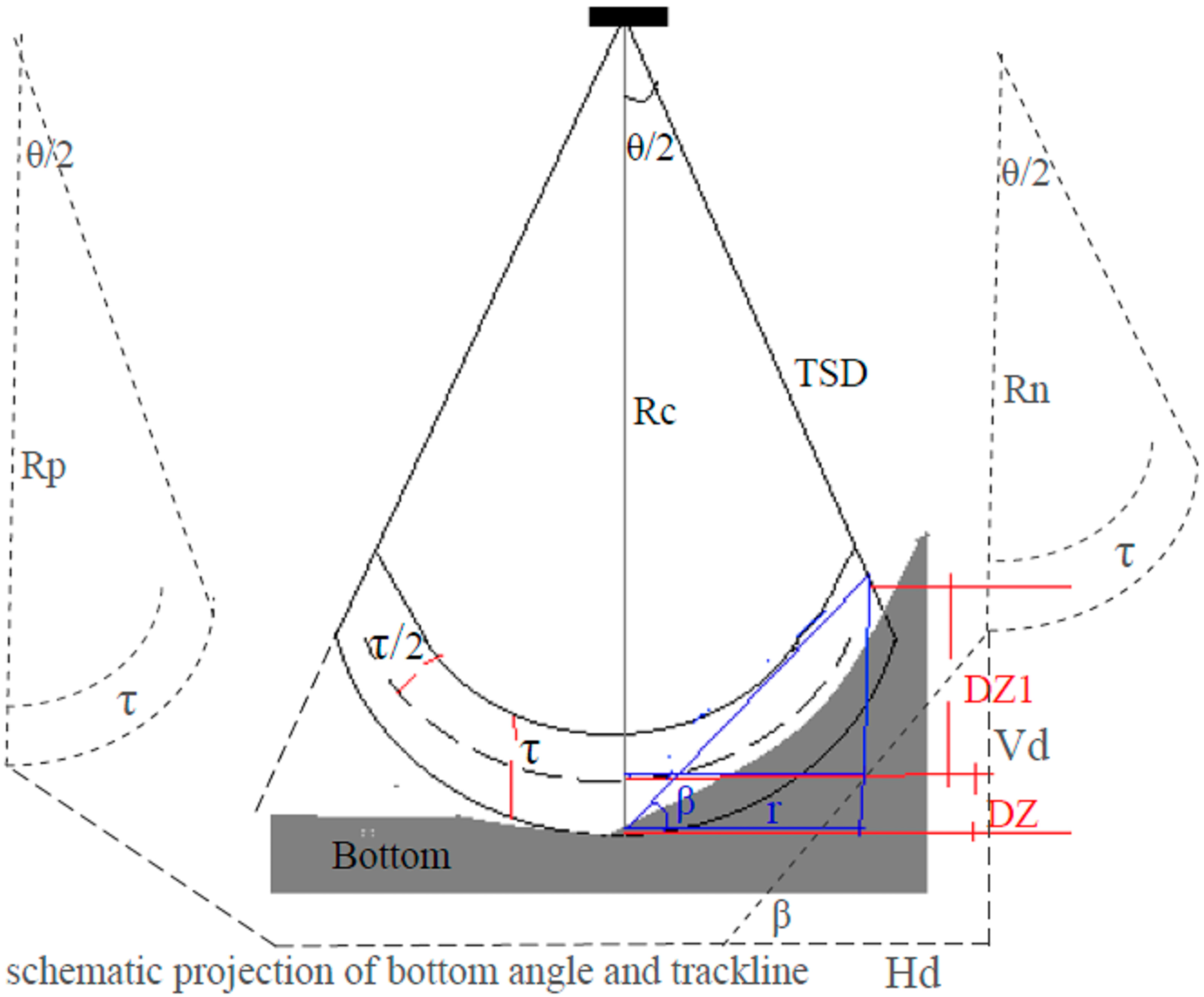
Figure 2.
Acoustic data profile versus depth (see Figure S1) for estimates of expected SNRb (a) and SNRir (b). The red line indicates Sv without TVG, the blue line indicates Sv with TVG and the green line indicates the regression curve.
Figure 2.
Acoustic data profile versus depth (see Figure S1) for estimates of expected SNRb (a) and SNRir (b). The red line indicates Sv without TVG, the blue line indicates Sv with TVG and the green line indicates the regression curve.

Figure 3.
An example file or data for the calibration of the meadow; raw data (a), removal of weak scatterers (b), removal of strong scatterers (c), removal and filtering of leaves (red continuous line denotes the ground and green the dead zone) (d) and vertical rhizomes and sheaths (e) on the enhanced echogram.


Figure 4.
Sequence of estimation of leaf length and biomass of the meadow in the main menu, POSIBIOM (a) and detailed flowchart of POSIBIOM (b). Numbers in the chart denote sequence of the processing. Dashed line denotes subcalls (algorithms) executed in linkage to main menu, POSIBIOM.
Figure 4.
Sequence of estimation of leaf length and biomass of the meadow in the main menu, POSIBIOM (a) and detailed flowchart of POSIBIOM (b). Numbers in the chart denote sequence of the processing. Dashed line denotes subcalls (algorithms) executed in linkage to main menu, POSIBIOM.


Figure 5.
Graphical menu for control, configuration and information of “Lost Bottom” (see Table S1 for the actions of each coded option and function with numbers).
Figure 5.
Graphical menu for control, configuration and information of “Lost Bottom” (see Table S1 for the actions of each coded option and function with numbers).

Figure 6.
Graphical menu for control, configuration and information of “Noise & Reverberation” (see Table S2 for actions of each coded option and function with numbers).
Figure 6.
Graphical menu for control, configuration and information of “Noise & Reverberation” (see Table S2 for actions of each coded option and function with numbers).

Figure 7.
Graphical outputs of the “Noise & Reverberation” analysis. (a) Enhanced echogram before the start of the analysis, (b) an algorithm to figure out the detection of the total noise, spurious echoes (optional), (c) the SNR for each background natural and artificial noise (optional) and (d) removed noise and reverberations; in this example, the configuration needed to be optimized to remove the total reverberations.

Figure 8.
Graphical menu for control, settings and info menu of “SheathFinder & Leaf and Biomass” (see Table S3 for actions of each coded option and function with numbers).
Figure 8.
Graphical menu for control, settings and info menu of “SheathFinder & Leaf and Biomass” (see Table S3 for actions of each coded option and function with numbers).


Figure 9.
Fixation and estimation of seagrass leaves during the analysis of acoustic data with “SheathFinder& Leaf and Biomass”; (a) scanning of sheaths or vertical rhizomes with green vertical line to determine false or real seagrass, (b) estimation of seagrass after the analysis of the current file was finished (green line denotes the canopy height) and (c) results table when checking the option (option no. 25 in Figure 8).


Figure 10.
Three-dimensional demonstration (latitude, longitude and depth) of the efficiency of the algorithm “Lost Bottom and Dead Zone” in recovering the real bottom and depth with the dead zone estimates in July 2011 (a), September 2011 (b), January 2012 (c) and April 2012 (d). The black line shows the bottom depth estimated with the Visual Analyzer program, and the green line shows the bottom depth corrected with the algorithm of this study. Vertical lines indicate errors with overestimates and underestimates on the acoustic trackline.

Figure 11.
Removal of background noise; different patterns of interferences. (a–c) Original data and (a’–c’) removal of interferences, respectively. Removal of background noise and reverberations; different patterns of surface and volume reverberations produced by SCUBA divers, (d) original data and (d’) removal of reverberations.


Figure 12.
Interpolated estimate of leaf biomass distribution (g/m2) in July 2011 (a), December 2011 (b), January 2012 (d) and April 2012 (e), and meters of leaf length in December 2011 (c) and April 2012 (f). X label (longitude); Y label (latitude).
Figure 12.
Interpolated estimate of leaf biomass distribution (g/m2) in July 2011 (a), December 2011 (b), January 2012 (d) and April 2012 (e), and meters of leaf length in December 2011 (c) and April 2012 (f). X label (longitude); Y label (latitude).


Disclaimer/Publisher’s Note: The statements, opinions and data contained in all publications are solely those of the individual author(s) and contributor(s) and not of MDPI and/or the editor(s). MDPI and/or the editor(s) disclaim responsibility for any injury to people or property resulting from any ideas, methods, instructions or products referred to in the content. |
© 2023 by the author. Licensee MDPI, Basel, Switzerland. This article is an open access article distributed under the terms and conditions of the Creative Commons Attribution (CC BY) license (https://creativecommons.org/licenses/by/4.0/).
Share and Cite
MDPI and ACS Style
Mutlu, E. A Package of Script Codes, POSIBIOM for Vegetation Acoustics: POSIdonia BIOMass. J. Mar. Sci. Eng. 2023, 11, 1790. https://doi.org/10.3390/jmse11091790
AMA Style
Mutlu E. A Package of Script Codes, POSIBIOM for Vegetation Acoustics: POSIdonia BIOMass. Journal of Marine Science and Engineering. 2023; 11(9):1790. https://doi.org/10.3390/jmse11091790
Chicago/Turabian StyleMutlu, Erhan. 2023. "A Package of Script Codes, POSIBIOM for Vegetation Acoustics: POSIdonia BIOMass" Journal of Marine Science and Engineering 11, no. 9: 1790. https://doi.org/10.3390/jmse11091790
Note that from the first issue of 2016, this journal uses article numbers instead of page numbers. See further details here.