Artificial Neural Network-Based Prediction of the Extreme Response of Floating Offshore Wind Turbines under Operating Conditions

Abstract

The development of floating offshore wind turbines (FOWTs) is gradually moving into deeper offshore areas with more harsh environmental loads, and the corresponding structure response should be paid attention to. Safety assessments need to be conducted based on the evaluation of the long-term extreme response under operating conditions. However, the full long-term analysis method (FLTA) recommended by the design code for evaluating extreme response statistics requires significant computational costs. In the present study, a power response prediction method for FOWT based on an artificial neural network algorithm is proposed. FOWT size, structure, and training algorithms from various artificial neural network models to determine optimal network parameters are investigated. A publicly available, high-quality operational dataset is used and processed by the Inverse First Order Reliability Method (IFORM), which significantly reduces simulation time by selecting operating conditions and directly yielding extreme response statistics. Then sensitivity analysis is done regarding the number of neurons and validation check values. Finally, the alternative dataset is used to validate the model. Results show that the proposed neural network model is able to accurately predict the extreme response statistics of FOWT under realistic in situ operating conditions. A proper balance was achieved between prediction accuracy, computational costs, and the robustness of the model.

1. Introduction

FOWT has consistently advanced in recent years, bringing with it not only more environmentally friendly engineering applications but also financial rewards and scientific advancements [1]. China, Japan, Portugal, Norway, and the UK will make up the top five markets for floating wind projects as of 2022 [2]. Since most wind energy is found in deep water, FOWT technology is advancing quickly [3]. Tension leg platform (TLP), Spar, semi-submersible (Semi), and barges are the three primary types of floating wind foundations now in use [4]. However, as offshore development activities move further out into the ocean, FOWT will produce stronger structural vibrations when subjected to more demanding environmental loads, which could cause instability issues and significant fatigue damage to the FOWT structure and anchor cables [5]. The motion response of a FOWT happens in six degrees of freedom (6DOF), which presents difficult design and evaluation problems [6]. Effectively lowering the likelihood of accidents in the system is real-time or advance prediction of the dynamic response of the FOWT system, which provides early warning of risky circumstances.

It is necessary to calculate the structure’s long-term severe reaction or loading for a specific recurrence period (once every 20 or 50 years) for any form of offshore structure, including the FOWTs [7]. The approach known as Full Long-term Analysis (FLTA) is thought to be the most accurate one for determining how maritime constructions will react to extremely high loads [8]. However, FLTA mandates simulation computations for at least 3000 different environmental scenarios, even if only a small number of them significantly affect how the structure responds. The Inverse First-Order Reliability Method (IFORM) is a well-liked technique to evaluate the ultimate loads of maritime structures with multidimensional variables and complicated nonlinear systems in order to minimize the number of simulations. IFORM was used to evaluate an oil tanker’s dependability in various sea situations [9]. It does not take a lot of calculations to estimate the joint long-term probability distributions of various FOWT severe loads using the IFORM [10]. IFORM is also featured among the dependability techniques outlined and assessed for the design of ships and offshore buildings [11].

The FOWT is a strongly nonlinear system, and its dynamic response is usually forecasted using a time-domain coupled analysis method. This method is computationally intensive, inefficient, requires expensive storage space and computer time, and is inconvenient for quickly obtaining the system response or forecasting ahead of time. In order to obtain the extreme response of FOWT quickly, some researchers have improved the time-domain coupling analysis method [12]. Research is being done on simplified and equivalent wave condition approaches that can decrease the number of computational conditions and increase the computational effectiveness of time domain evaluation methods [13,14]. Additionally, real-time simulation methods are employed to track how the FOWT’s structural performance responds to varied wind and wave loads [15,16]. Although the computational effectiveness or reaction times of these systems have increased, they are still unable to accommodate the need for brief delays in actual use.

Some researchers have used artificial neural networks in the discipline of marine engineering as a result of the development of big data and artificial intelligence [17]. The ANN algorithm, which has great computational efficiency and produces precise results, simply has to concentrate on the significant nonlinear relationship between the inputs and outputs. As a result, it is frequently utilized. An enhanced radial basis function (RBF) neural network strategy is provided for torque management of the FOWT system at speeds lower than the rated wind speed. This approach targets the external disturbances and nonlinear uncertain dynamic systems of the FOWT due to the proximity to load centers and strong wave coupling [18]. Artificial neural network-based fuzzy logic control enhances the dynamic behavior of the FOWT platform and boosts its stability under a variety of wind and wave situations [19]. An intelligent damage detection framework on FOWT was created using a multi-scale deep convolutional neural network model. The framework’s performance is at least 10% better than the diagnostic precision attained with the majority of popular industrial-grade diagnostic tools [20]. The results demonstrate the possibility of including artificial neural networks in the mooring design process. Artificial neural networks were used to simulate the time course of FOWT mooring tension in a range of irregular wave sea conditions [21].

As a result of their high inference accuracy, flexibility, resilience, fault tolerance, adaptability, scalability, generalization, and extrapolation capabilities in several successful applications, artificial neural network-based models have generally been shown to be more accurate in prediction [22]. In research fields including FOWT behavioral control, fault analysis, generating power prediction, and dynamics modeling, machine learning is presently being employed more. There are, however, few techniques for accurately forecasting the FOWT systems’ severe dynamic response values. As a result, a model for predicting extreme responses for FOWT enterprises is built in this research using artificial neural networks. To improve the accuracy of predicting FOWT extreme responses, the performance of shallow and deep ANN models with various dimensions is investigated, as is the impact of various network structures and the use of various training algorithms on ANN model performance and computational complexity. Artificial neural networks require a lot of input data to be trained, and the quality and quantity of that data directly impact the training outcomes. So, by processing marine environmental data from the TRL+ National Research Program (Spain) using IFORM, a sizable amount of training data was acquired. Additionally, a sensitivity study was carried out to look at the impact of changing the validation check values or the number of neurons on the model’s ability to predict outcomes accurately. In order to explore the generated ANN model’s generalizability and accuracy, the forecasting model’s dependability was also confirmed.

2. Methodology

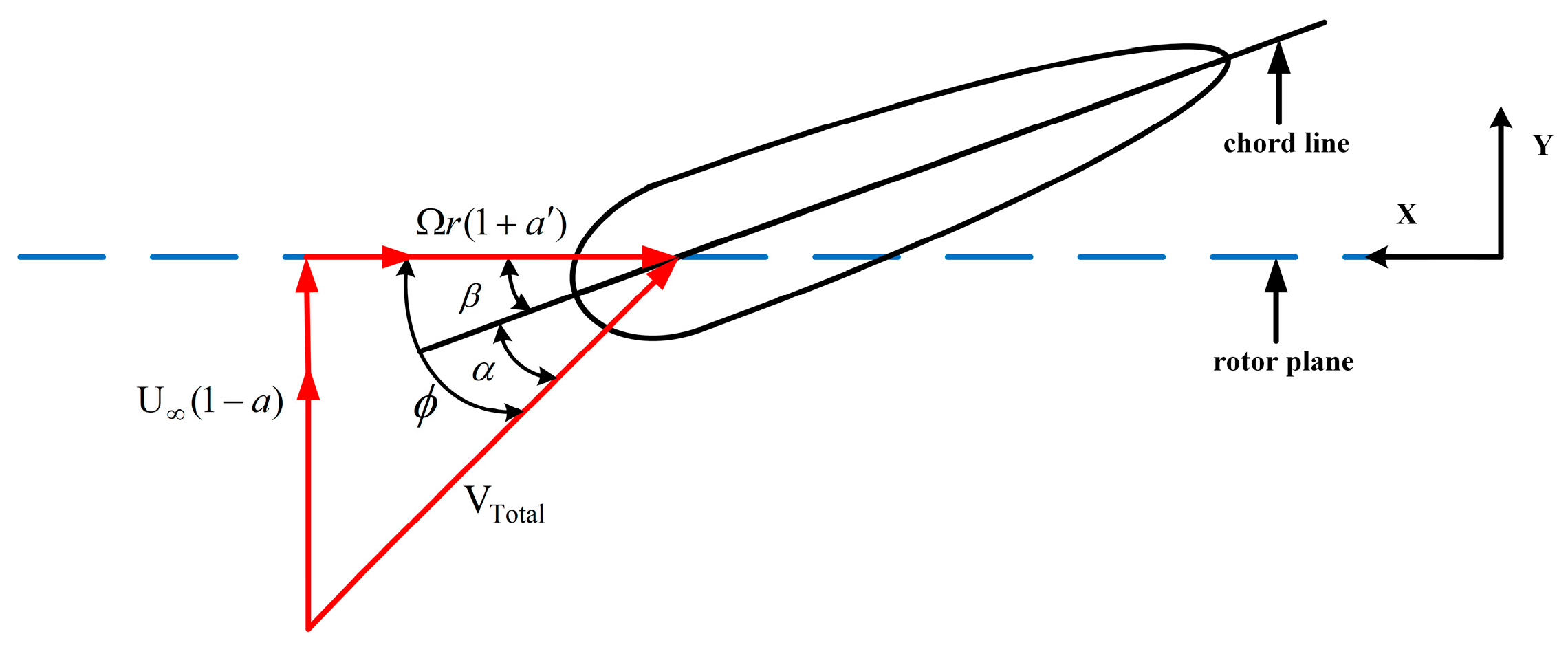
2.1. Aerodynamic Load

The Blade Element Momentum Theory (BEM), which consists of the momentum theory and the blade element theory, is one of the primary techniques for estimating the aerodynamic stresses on wind turbine blades. According to the blade element hypothesis, the blade is divided into foliation units that are all infinitely thin and independent of one another [23]. Figure 1 shows an illustration of an airfoil with the speeds and angles that define the forces acting on the element as well as the induced speeds brought on by the effect of the wake. Mathematical modeling of aerodynamic loads will be undertaken by AeroDyn [24].

The two components of the local velocity vector yield the angle of inflow [25].

$$\tan \phi =\frac{U_{\infty }(1-a)}{\Omega (1+a^{\prime })}=\frac{(1-a)}{(1+a^{\prime }){\lambda }_r}$$

(1)

where $\phi$ denotes the angle of incidence; $U_{\infty }$ the speed of the entering wind at infinity; $a$ the axial induction factor, and $a^{\prime }$ the tangential induction factor; $\Omega$ stands for the wind turbine’s angular velocity; $r$ for its foliation to hub center distance; and ${\lambda }_r$ for its regional tip speed ratio.

By incorporating the vane’s aerodynamic properties throughout the radius, the wind turbine’s aerodynamic properties are determined. Figure 2 depicts the resulting aerodynamic forces on the element and its parts, both perpendicular to the rotor plane and parallel to it. The axial thrust $\mathrm{d}T$ and torque $\mathrm{d}Q$ on a blade element micro-segment with distance $r$ from the leaf root and thickness $\mathrm{d}r$ are as follows [26,27]:

$$\mathrm{d}T=\frac{1}{2}B\rho c{v}_0^2(C_L\cos \phi +C_D\sin \phi )\mathrm{d}r$$

(2)

$$\mathrm{d}Q=\frac{1}{2}B\rho c{v}_0^2(C_L\sin \phi -C_D\cos \phi )\mathrm{d}r$$

(3)

In this equation, $B$ stands for the number of blades, $\rho$ for air density, $c$ for air density, $v_0$ for relative incoming velocity, $C_L$ for lift coefficient, $\phi$ for incidence angle, and $C_D$ for drag coefficient.

The relationship between the forces and moments acting on the wind turbine and the momentum and angular momentum is established by the momentum theory, which assumes that the loss of pressure or momentum in the plane of the wind turbine is caused by the work done by the airflow in the plane of the wind turbine on the blade element. The following describes the axial thrust $\mathrm{d}T$ and torque $\mathrm{d}M$ on a micro-segment of the vane located at a point $r$ away from the vane’s root and having a thickness $\mathrm{d}r$ [26,27].

$$\mathrm{d}T=4\pi \rho v_1^{2}a(1-a)r\mathrm{d}r$$

(4)

$$\mathrm{d}Q=4\pi \Omega v_1^{}b(1-a)r^3\mathrm{d}r$$

(5)

In this scenario, $v_1$ denotes the entering velocity, $a$ the axial induction factor, and $b$ the tangential induction factor. The iterative technique may be used to calculate the force, torque, and power operating on the wind turbine’s wind wheel in conjunction with the Blade Element Theory and momentum theory.

2.2. Hydrodynamic Load

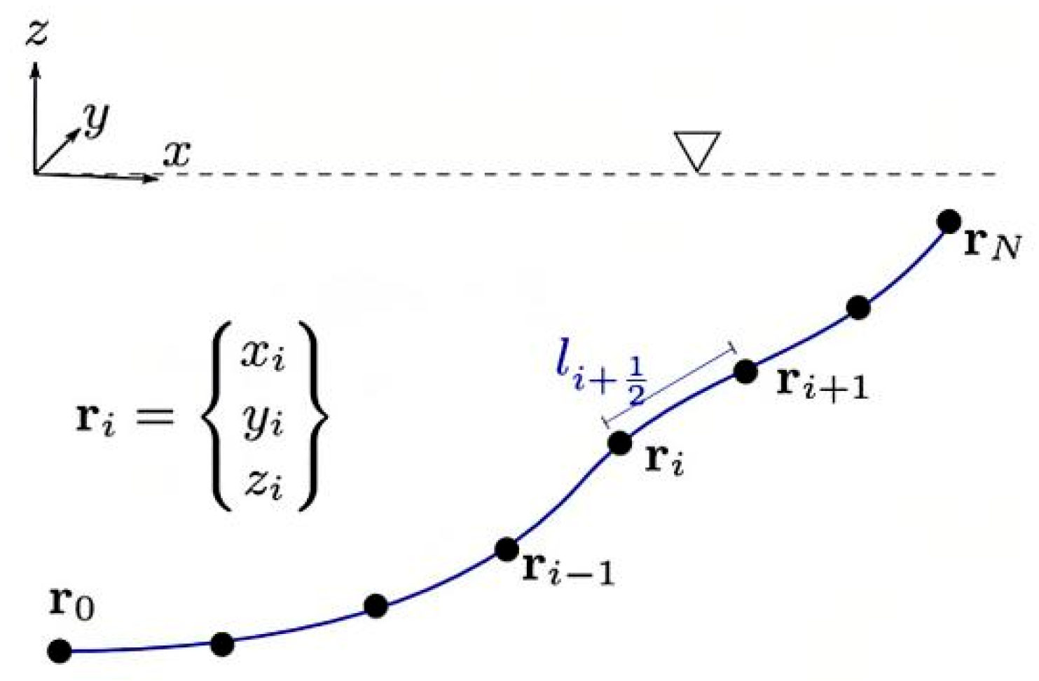
In particular, the 3D potential flow theory is utilized to solve for the wave stresses on the floating foundation for large-scale constructions ($D/L>0.2$, $D$ represents the diameter of the circular member, and $L$ signifies the wavelength) [28], as illustrated in Equation (6). For small-scale structures ($D/L<0.2$), Morrison’s equations are used to solve the wave loads for slender structures, as shown in Equation (7) [29]. Mathematical modeling of hydrodynamic loads will be undertaken by HydroDyn [30].

$$F_i^h(t)=F_i(t)-{\displaystyle {\int }_0^t{K}_{ij}(t-\tau ){\dot{\xi }}_j(\tau )d\tau }-A_{ij}{\ddot{\xi }}_j+\rho g{V}_0{\delta }_{i3}-C_{ij}^h{\xi }_j$$

(6)

where $F_i(t)$ is diffraction force, $-{\displaystyle {\int }_0^t{K}_{ij}(t-\tau ){\dot{\xi }}_j(\tau )d\tau }-A_{ij}{\ddot{\xi }}_j$ is radiation force and $\rho g{V}_0{\delta }_{i3}-C_{ij}^h{\xi }_j$ is hydrostatic force.

$$dF(t)=\rho A\dot{u}+\rho A{C}_m(\dot{u}-{\ddot{\xi }}_j)+\frac{\rho }{2}D{C}_d(u-{\dot{\xi }}_j)\left|u-{\dot{\xi }}_j\right|$$

(7)

where $A$ represents the cross-sectional area of the elongated structure, $D$ represents the diameter, $\rho$ represents the seawater density, $u$ represents the velocity of the wave mass, $C_m$ represents the added mass, $C_d$ represents the drag coefficient, and $\xi$ is the amplitude of the wave height.

2.3. Mooring Load

As shown in Figure 3, the lumped mass method discretizes the mooring anchor chain into $n$ segments of uniformly equal length with massed nodes and massless spring damping, which are connected through $n+1$ nodes to form the mooring anchor chain [31]. The mathematical modeling of the lumped mass method will be undertaken by MoorDyn [32].

This technique has the benefit of accounting for the cable’s self-weight and buoyancy as well as the dynamic impacts of current drag and inertia forces. The publication provides a thorough explanation of how the equations were derived [33], and only the dynamic equations of each node are given here as follows:

$$(m_i+a_i){\ddot{r}}_l=F_{T_{i+1/2}}-F_{T_{i-1/2}}+C_{{}_{i+1/2}}-C_{{}_{i-1/2}}+W_i+F_B+F_{D_{pi}}+F_{D_{qi}}$$

(8)

where $m_i$ and $a_i$ stand for the mass and added mass of each node, respectively; $F_{T_{i+1/2}}-F_{T_{i-1/2}}+C_{i+1/2}-C_{i-1/2}$ for the internal stiffness and damping force; $W_i+F_B$ for gravity and the force of contact with the seafloor; and $F_{D_{pi}}+F_{D_{qi}}$ for the drag force at each node.

3. Numerical Simulations of FOWT Loads

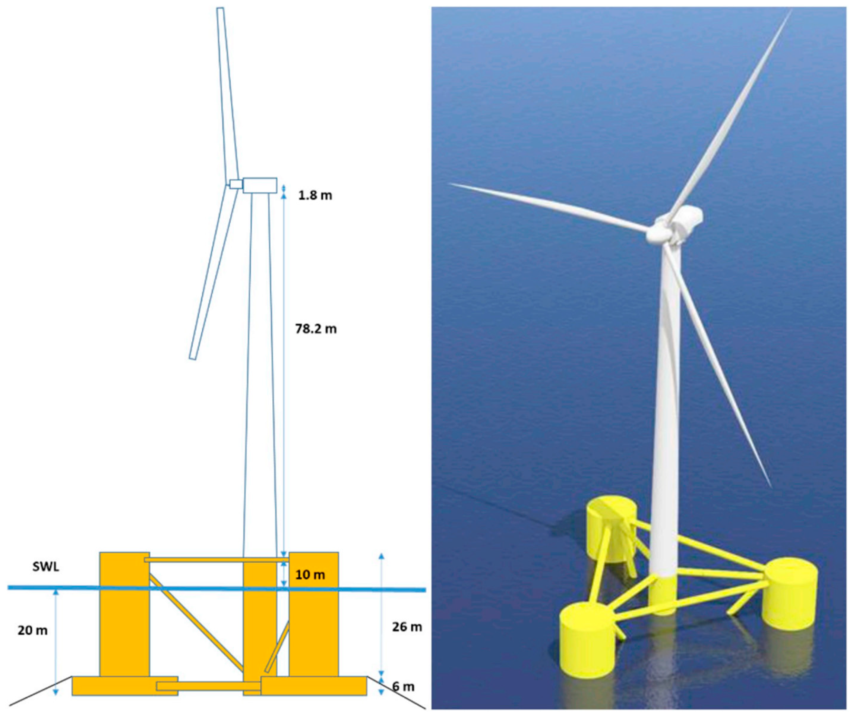
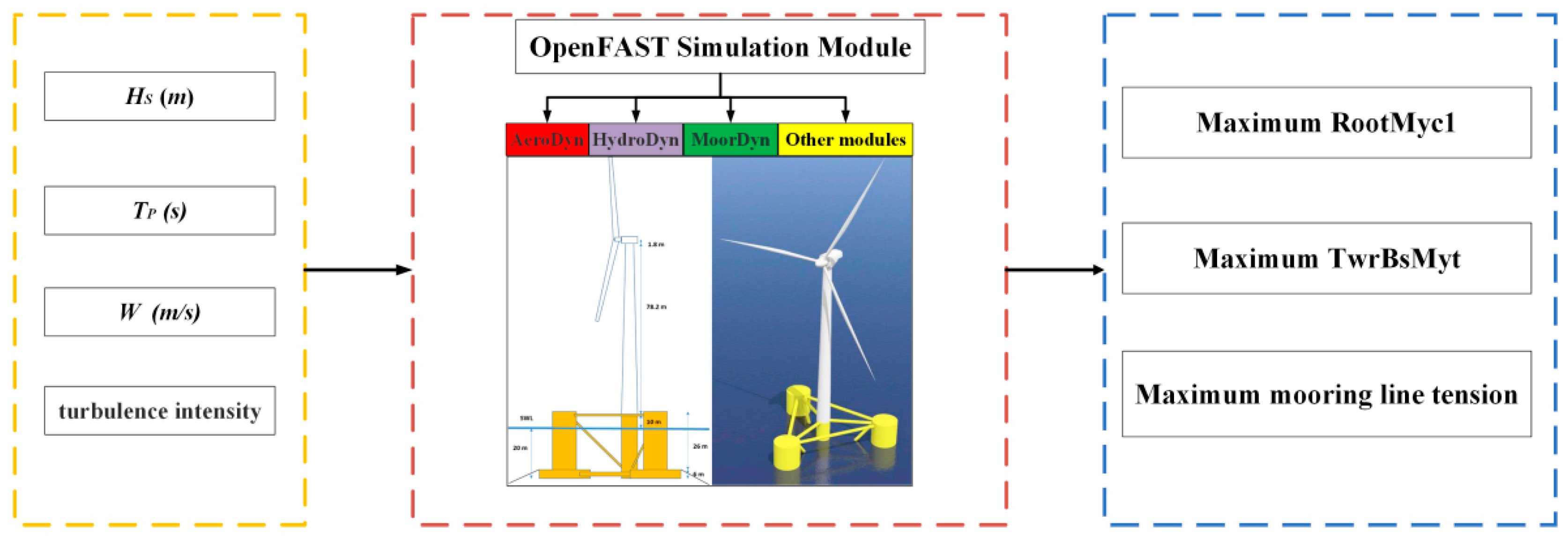
3.1. Description of the FOWT Model

The NREL 5MW horizontal axis wind turbine model is depicted in Figure 4. It was developed using data from numerous wind power research and development projects and is now widely used in the field of research pertaining to wind power. Table 1 lists the key wind turbine parameters.

Semi-submersible FOWTs will be the focus of future development due to their short draft and outstanding stability, according to the U.S. Offshore Wind Technology Market Report [3]. The support platform, as seen in Figure 4, primarily consists of a central column, three offset outside columns, and several thin supports. The primary characteristics of the DeepCwind semi-submersible platform are listed in

Table 2. DeepCwind semisubmersible platform, data are from [36].

Platform Properties	Value
Platform draft	20.0 m
Centerline spacing between offset columns	50.0 m
Length of upper columns	26.0 m
Length of base columns	6.0 m
Diameter of main column	6.5 m
Diameter of offset (upper) columns	12.0 m
Diameter of base columns	24.0 m
Diameter of pontoons and cross braces	1.6 m

. The three mooring anchor chains are evenly spaced along the axial direction of the middle short columns, and one end of each mooring chain is connected to the edge short columns through the guide holes and anchored to the seabed at the other end. The mooring anchor chain uses a suspension chain line type to provide the restoring force. In this study, more information on the mooring chain is provided [35].

Table 1. Main parameters of NREL 5MW wind turbine, data are from [36].

Turbine Properties	Value
Rotor configuration	Upwind, 3 Blades
Cut-in wind speed	3 m/s
Rated wind speed	11.4 m/s
Cut-out wind speed	25 m/s
Rotor mass	110,000 kg
Nacelle mass	240,000 kg
Tower mass	347,460 kg

Table 1. Main parameters of NREL 5MW wind turbine, data are from [36].

Turbine Properties	Value
Rotor configuration	Upwind, 3 Blades
Cut-in wind speed	3 m/s
Rated wind speed	11.4 m/s
Cut-out wind speed	25 m/s
Rotor mass	110,000 kg
Nacelle mass	240,000 kg
Tower mass	347,460 kg

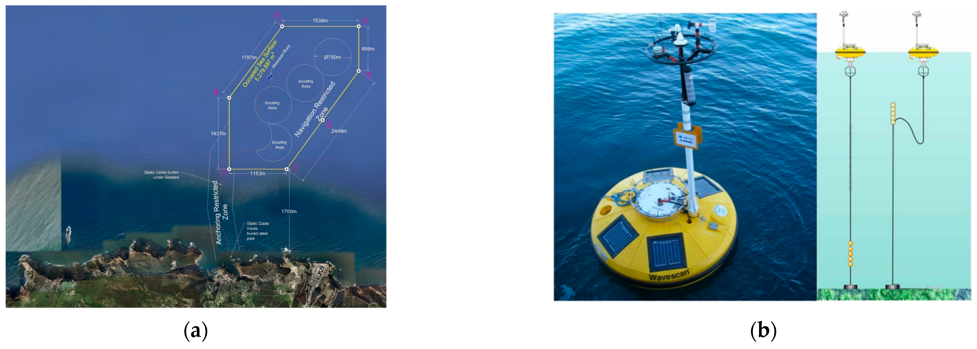
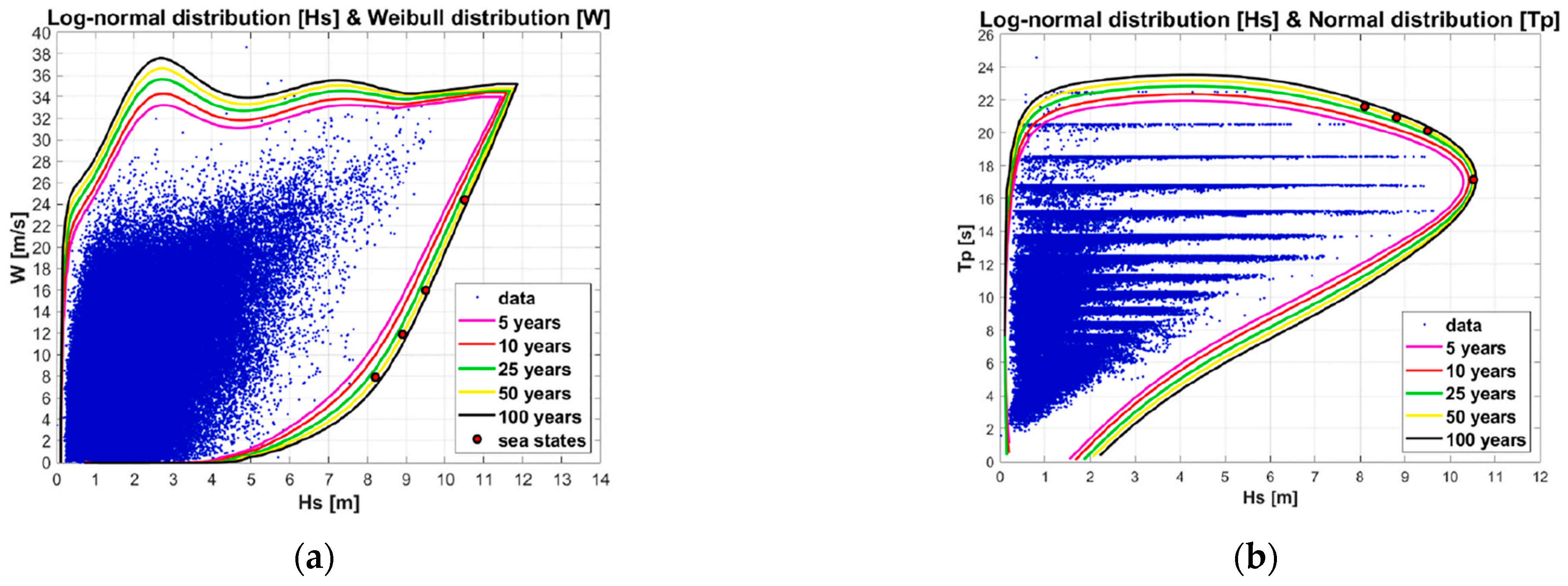
3.2. Marine Environmental Data

The open-ocean test facility BiMEP, which is 2 km offshore of the Spanish coastal town of Armintza, provided the data utilized in this simulation. The BiMEP test center, which has a total surface area of 5.2 km² and depths ranging from 50 to 90 m, is depicted in Figure 5a. The WAVESCAN directional buoys set up at BiMEP will gather marine meteorological data (currents, winds, and waves) and send it in real time to coastal stations through satellite communications, as illustrated in Figure 5b.

In this work, the Inverse First Order Reliability Method (IFORM) is used to identify the severe sea state, and greater emphasis is placed on the accurate prediction of wind turbine loads in severe sea conditions [39], which can obtain maritime meteorological conditions over a long period. IFORM is used to create environmental contours on which design circumstances are chosen to compute the reaction, greatly cutting down on the simulation time [40]. IFORM was used to analyze data from the TRL+ National Research Project to determine the effects of long-term severe sea conditions on FOWTs [37,38], and Figure 6 displays the wave characteristics and the distributions of wind speed parameters (90 m above sea level).

Considering the offshore standard [41], the four loading conditions were chosen from the 50-year environmental contour (yellow) in Figure. 6 because the maritime environment chosen for the FOWT must have a return duration of 50 years. Separating the datasets correctly can increase the artificial neural network’s dependability [42]. The neural network model must be trained on a huge volume of data, and by discretizing the aforementioned four working conditions, additional environmental factors may be gained.

For example, in the meaningful wave height interval $H_S\in (8.10,8.81)$, the step size $t=0.05$ is taken to generate 14 groups of meaningful wave height working conditions. In order to obtain 14 sets of wind speed conditions matching the meaningful wave height, the appropriate step size is taken through the wind speed interval $W\in (7.93,11.93)$. By analogy, another 29 groups of wind and wave loading data are obtained at $H_S\in (8.10,9.50)$, $W\in (11.93,16.08)$ and $H_S\in (9.50,10.30)$, $W\in (16.08,25.69)$. The total number of wind and wave conditions is 43.

To cover the spectral peak periods of short, medium, and long bands in the marine environment, three spectral peak periods were designed, namely 6 s, 12 s, and 24 s. In order to investigate the effect of different turbulence intensities on the load response of the floating wind turbine, three turbulence intensities were designed with reference to the requirements of the International Electrotechnical Commission (IEC) [43], which are 0.16, 0.14, and 0.12. With 43 wind and wave loading data available, 43 × 3 × 3 environmental parameters were obtained by considering three different spectral peak periods and turbulence intensities and were divided into three data sets, as shown in

Table 3. Environmental loading conditions for neural network training.

${\mathbf{H}}_{\mathbf{S}}\left(\mathbf{m}\right)$	${\mathbf{T}}_{\mathbf{P}}\left(\mathbf{s}\right)$	$\mathbf{W} (\mathbf{m}/\mathbf{s})$	Turbulence Intensity (IEC)	Working Condition Number	Dataset Number
8.1–8.81	6, 12, 24	7.93–11.93	0.16, 0.14, 0.12	1–126	1
8.81–9.50	6, 12, 24	11.93–16.08	0.16, 0.14, 0.12	127–243	2
9.50–10.30	6, 12, 24	16.08–25.69	0.16, 0.14, 0.12	244–387	3

.

3.3. Load Simulation Calculation

A tool called OpenFAST [44] can simulate the coupled dynamic response of wind turbines using several physics models and levels of accuracy. To enable coupled nonlinear aero-hydro-servo-elastic modeling in the time domain, OpenFAST joins computational modules for aerodynamics, hydrodynamics for offshore structures, control and electrical system (servo) dynamics, and structural dynamics. As shown in Figure 7, AeroDyn [24], HydroDyn [30], and MoorDyn [32] in OpenFAST are responsible for calculating blade aerodynamic loads, hydrodynamic loads, and mooring loads, respectively. The FOWT coupled system dynamics model is established based on the above functional modules. In fact, other functional modules of OpenFAST are also involved in the computation, and the details can be found in this paper [44].

A stochastic, full-field turbulent wind model is TurbSim [45]. It simulates a three-component windspeed time series numerically at locations in a fixed, two-dimensional vertical rectangular grid using a statistical model. The turbulent wind field was generated using TurbSim. Referring to the turbulence intensity mentioned in the preceding section, choose the Kaimal turbulent wind spectrum and the NTM wind load model.

The full turbine dynamics simulation took ten minutes. To avoid being impacted by the FOWT’s transitory behavior during startup, the simulation time was extended to 630 s, omitting the first 30 s, and the time step was changed to 0.0125 s. As shown in Figure 8, the blade root out-of-plane bending moment, tower base fore-aft bending moment, and mooring line tension of the FOWT in Condition 1 were obtained according to the above setup. All sea states are calculated, and the maximum value of the dynamic response is counted. Later, a neural network prediction model is developed using the environmental parameters as inputs and the maximum value of the dynamic response as outputs.

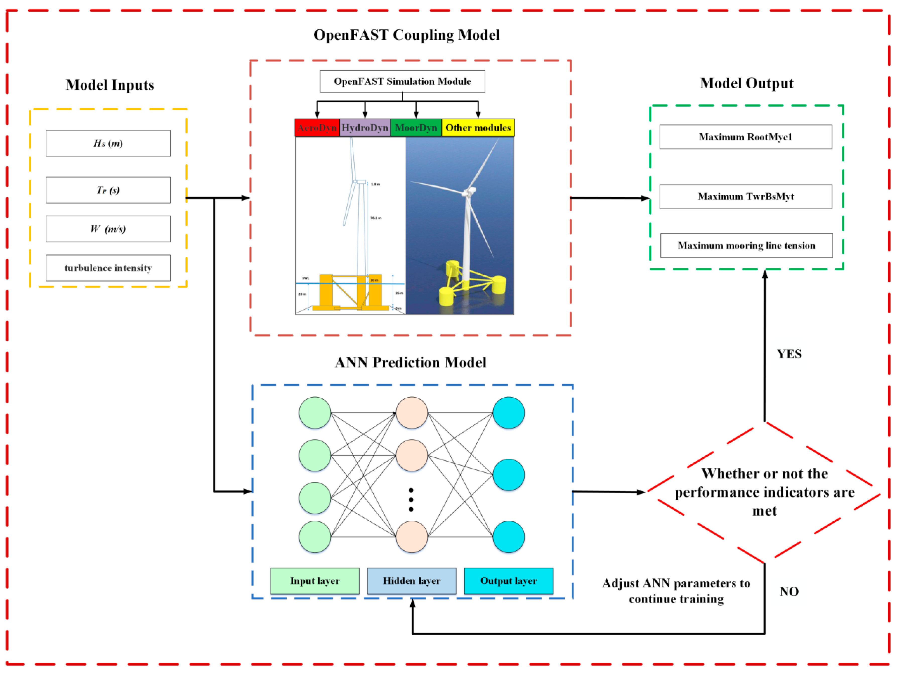
4. Artificial Neural Network Predictive Modeling

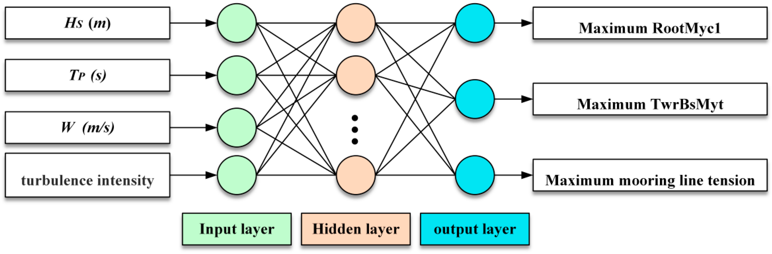
4.1. Artificial Neural Network Framework

In all varieties of artificial neural networks, the input, hidden, and output layers are all combined into a multi-layer feed-forward (MLFF) structure. It is the neural network structure of this paper, as seen in Figure 9. The maximum value of the blade root out-of-plane bending moment, the maximum value of the tower base fore-aft bending moment, and the maximum value of mooring line tension are selected as the model’s output parameters. Wind speed, turbulence intensity, meaningful wave height, and spectral peak period are chosen as the model’s input parameters.

Let the input $x={(x_1,x_2,\cdots ,x_n)}^{\mathrm{T}}$, totaling $n$ layer, and the implicit layer output be the output layer input $y={(y_1,y_2,\cdots ,y_h)}^{\mathrm{T}}$, totaling $h$ layer. Output layer $z={(z_1,z_2,\cdots ,z_m)}^{\mathrm{T}}$, totaling $m$ layers, $w_{ij}$ and ${\theta }_{ij}$ denote the weights and thresholds from the $i$ neuron in the input layer to the $j$ neuron in the hidden layer, and $w_{jk}$ and ${\theta }_{jk}$ denote the weights and thresholds from the $j$ neuron in the hidden layer to the $k$ neuron in the output layer, respectively, $i=(1,2,\cdots ,n)$, $j=(1,2,\cdots ,h)$, $k=(1,2,\cdots ,m)$.The activation function from the input layer to the hidden layer is $f$, and the activation function from the hidden layer to the output layer is $g$. The process of signal smooth propagation is essentially the process of obtaining the output result by calculating the activation function, and the output $z_k$ of the $k$ neuron in the output layer is as follows:

$$z_k=g({\displaystyle \sum _{j=1}^h{w}_{jk}}{y}_j+{\theta }_{jk})=g({\displaystyle \sum _{j=1}^h{w}_{jk}}f({\displaystyle \sum _{i=1}^n{w}_{ij}}{x}_i+{\theta }_{ij})+{\theta }_{jk})$$

(9)

One of the mechanical learning systems that uses strong learning from samples is an Artificial Neural Network (ANN), which can comprehend complicated nonlinear interactions [46]. In this study, a neural network known as a back propagation (BP) neural network that exhibits both forward and backward propagation of error correction is used. Currently, complicated nonlinear systems of marine structures frequently employ this feed-forward back-propagation neural network [47]. BP neural network uses error correction backward propagation, which first corrects the error from the output layer to the implicit layer before utilizing the gradient descent approach to change the weights and thresholds until the prediction of an artificial neural network closely resembles the desired outcome. Minimizing the mean square error of the desired value $t_k$ and the network output value $z_k$ is taken as the objective, and the mean square error (MSE) of the output layer is calculated as follows:

$$\mathrm{MSE}=\frac{1}{m}{\displaystyle \sum _{k=1}^m{(t_k-z_k)}^2}$$

(10)

The accuracy of the output results, training duration, and network convergence speed are all impacted by wind, waves, and other maritime environment factors, as well as by the vast numerical range of the eigenvalues of the dynamic response of the floating wind turbine system. As a result, before training the neural network, the data must be normalized. The bipolar activation function’s normalization formula is shown below.

$$\widehat{x}=\frac{2(x-x_{\min })}{x-x_{\max }}-1$$

(11)

with $\widehat{x}$ being the normalized data, and the data set’s minimum and maximum values are represented, respectively, by the letters $x_{\min }$ and $x_{\max }$.

The entire dataset was randomly separated into three subsets: a training set (70%), a validation set (15%), and a test set (15%) in order to prevent the overfitting issue [48,49]. Only the training dataset is used to train the network; the validation dataset is used to test the network’s generalizability and to stop the training process before it becomes overfit. The artificial neural network was independently tested using the test dataset.

A floating wind turbine is a complex dynamical system, and it is time-consuming to obtain the power response from modeling to calculation. As shown in Figure 10, artificial neural networks may be useful to accelerate FOWT power response predictions. The inputs to the extreme response forecasting model are the environmental parameters acting on the FOWT, and the output is the extreme response of the FOWT.

4.2. Training of Neural Networks

To make an accurate forecast, choosing the appropriate network topology and parameters is crucial [50,51]. In order to better understand how different artificial neural network characteristics, particularly the hidden layer network topology and training technique, affect prediction performance. Based on MATLAB, a BP neural network was created [52], and a series of activation functions and training functions were provided in the MATLAB toolbox. BP neural networks require the activation function to be derivable, so a bipolar activation function (tanning-sigmoid) is used as an implicit layer [53]. The output layer is a pure linear activation function (purelin) [54]. The training procedures for the other datasets are identical; however, in the following, training for dataset 1 will be used as an example. Twenty computations will be performed using the same network configuration, and the accuracy of the forecasted results will be assessed using the mean square error average. After the neural network’s fundamental structure has been established, it must be trained. Various training techniques will be used, and the results will be examined.

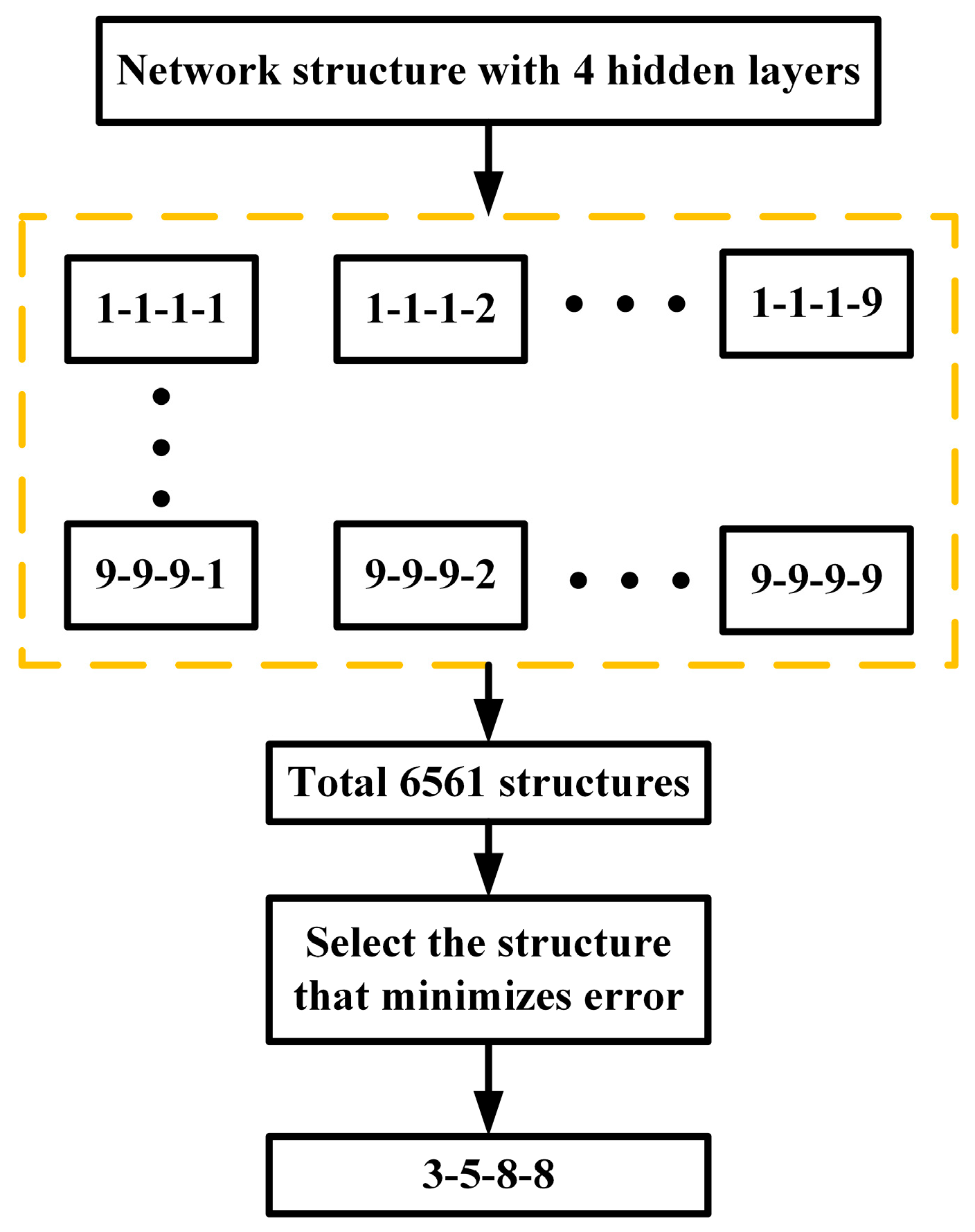
4.2.1. Hidden Layer Network Structure

The number of hidden layers and the number of neurons in each hidden layer together form the network structure. The network structure will have a significant impact on prediction accuracy. For the BP neural network, the number of hidden layers can be set arbitrarily, but in fact, the more hidden layers, the more complex the network structure will be, and the more complex the calculation will be. For most engineering problems, the neural network with one or two hidden layers can complete the fitting task of almost all mapping relations [55]. By changing the number of hidden layers and the number of neurons in each hidden layer, different network structures are obtained, and the accuracy of the prediction model under the network structure is calculated. In order to determine the number of hidden layers, neural networks with 1, 2, 3, and 4 hidden layers were tried, respectively. As shown in Figure 11, a neural network with four hidden layers has a maximum of nine neurons per layer, and there are a total of 6561 different network structures. In order to avoid contingency, each network structure needs to run 20 times to take the average, and finally, the network structure with the smallest error needs to be taken. The number of calculations is too large, so a batch file is written. The data set 1 was used for training. After calculation, the number of neurons with the smallest error under different hidden layers was obtained, as shown in

Table 4. The impact of hidden layer network structure on computational accuracy.

	Number of Hidden Layer Layers (Number of Neurons Per Layer)
Output Response	1(9)	2(4–9)	3(3–6–9)	4(3–5–8–8)
	MSE	MSE	MSE	MSE
Maximum RootMyc1	0.0128	0.0116	0.0127	0.0132
Maximum TwrBsMyt	0.0023	0.0020	0.0019	0.0022
Maximum mooring line tension	0.0012	0.0010	0.0010	0.0012
time consuming/s	4.37	5.89	7.45	8.72

.

By increasing the number of implied layers, the mean square error of the computed results of the power response prediction model is significantly reduced. Too many hidden layers can lead to the negative effect of overfitting. The maximum value of the mooring chain tension is much more accurately represented in the output response than are the maximum values of the external bending moments at the leaf root surface and the bending moments in front of and behind the tower base. The mean square error of the computed results of the power response prediction model is greatly decreased by increasing the number of assumed layers. Overfitting might be a problem if there are too many covert layers. The accuracy of the maximum value of the mooring line tension in the output response is much greater than that of the blade root out-of-plane bending moment and the tower base fore-aft bending moment.

As shown in Figure 12, the output of the forecasting model under the 2(4–9) network structure is compared with the expectation. The training, validation, and test sets’ respective regression coefficients are 0.99424, 0.98969, and 0.98614. A better fit is denoted by a bigger R. The created neural network model has a significant capacity for generalization, as evidenced by the regression coefficient R of all the dataset training reaching 0.99275 and the good agreement between the neural network projected value and the anticipated value.

4.2.2. Comparison of Training Algorithms

By using the network structure of three hidden layers as an example, different training algorithms’ effects on the accuracy of prediction models may be further examined. The first, second, and third layers of this network each contain 3, 6, and 9 neurons, respectively. The selection of different BP neural network training algorithms for prediction. The adaptive learning rate gradient descent method [56] and the scaled conjugate gradient backpropagation [57] are significantly more efficient compared to the most basic gradient descent method, but the computational accuracy does not meet the requirements; see

Table 5. Effect of different neural network algorithms on computational accuracy.

	Algorithm
Output Response	Gradient Descent	Gradient Descent with Adaptive Learning Rate	Scaled Conjugate Gradient	Bayesian Regularization	Levenberg–Marquardt
	MSE	MSE	MSE	MSE	MSE
Maximum RootMyc1	0.1295	0.1006	0.0433	0.0123	0.0119
Maximum TwrBsMyt	0.183	0.0794	0.0208	0.0024	0.0018
Maximum mooring line tension	0.2078	0.0823	0.0215	0.0012	0.0009
Time consuming/s	26.94	8.67	8.34	10.74	7.96

. Bayesian regularization [58] and Levenberg–Marquardt [59] with significantly higher computational accuracy. In reality, as rapid backpropagation techniques are highly advised as first-choice supervised algorithms, the Levenberg–Marquardt and Bayesian regularization backpropagation algorithms are considered the finest options for such nonlinear dynamics. For this simulation, Levenberg–Marquardt has no additional training time and is recommended as the neural network training algorithm for dynamic response prediction models.

5. Results and Discussion

First, the sensitivity of the model’s performance metrics to the number of neurons and the number of validations will be discussed. Then the network structure with the highest computational accuracy will be selected as the structure of the power response prediction model, and the reliability of the model will be verified with a new data set.

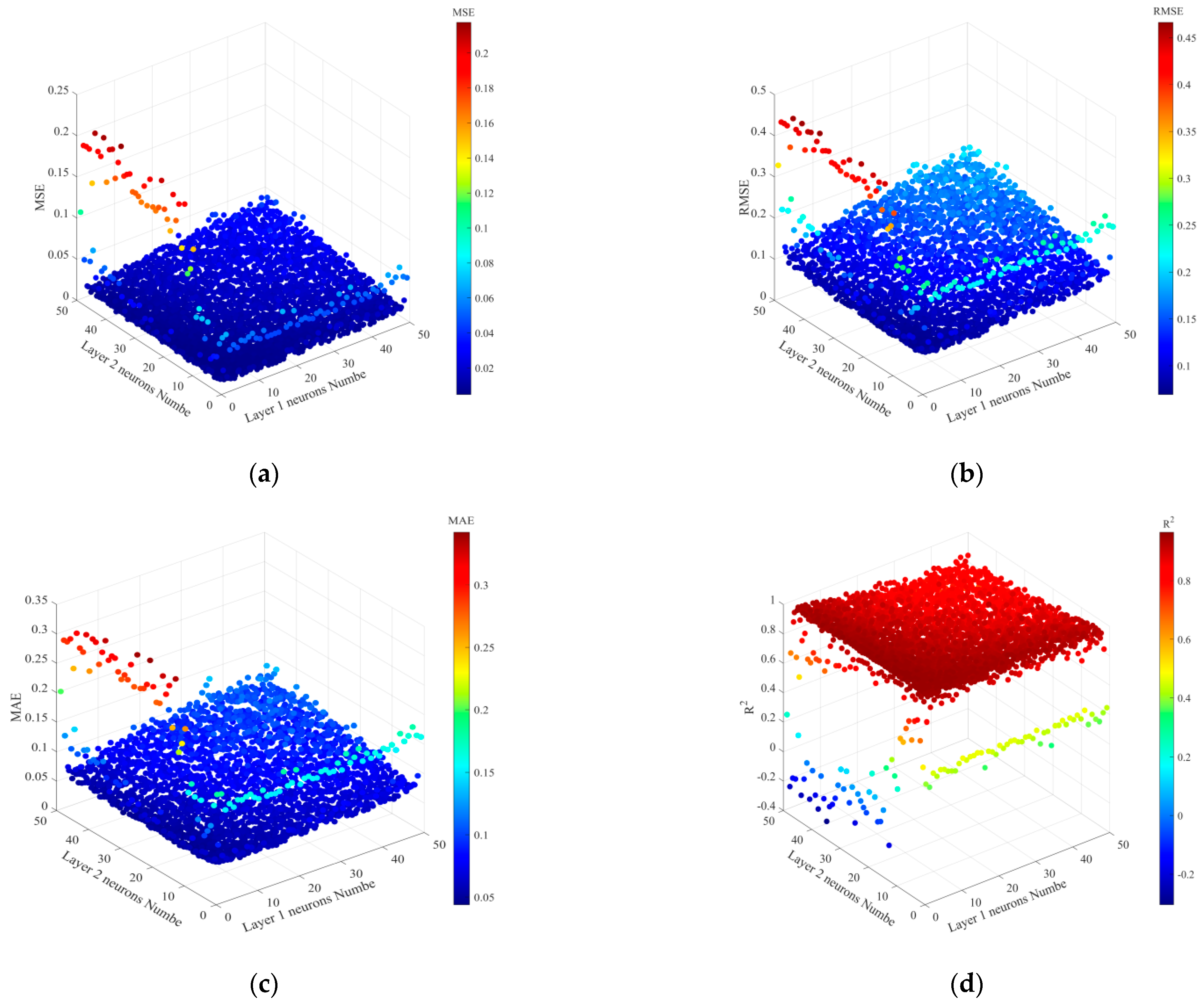
5.1. Sensitivity Analysis

Determination of the number of neurons is a more complex problem. In order to study the sensitivity of the neural network model performance to the number of neurons and the number of validations, three additional evaluation metrics, RMSE, MAE, and Coefficient of Determination R², were added. The three responses were evaluated as a whole without calculating the evaluation metrics for each response variable separately.

The root mean square error (RMSE) can be obtained by taking the square root of the MSE, which is more sensitive to larger error values.

$$\mathrm{RMSE}=\sqrt{\frac{1}{m}{\displaystyle \sum _{k=1}^m{(t_k-z_k)}^2}}$$

(12)

Mean Absolute Error (MAE) does not take into account the square of the variance, so it does not amplify the squared difference in the variance values and is more intuitive relative to MSE, which reflects the absolute magnitude of the prediction error rather than the squared magnitude of the error.

$$\mathrm{MAE}=\frac{1}{m}{\displaystyle \sum _{k=1}^m\left|t_k-z_k\right|}$$

(13)

Coefficient of Determination R², which indicates the proportion of variability in the dependent variable that can be explained by the model, and how well the model fits the data.

$${\mathrm{R}}^2=1-{\displaystyle \sum _{k=1}^m{(t_k-z_k)}^2}/{\displaystyle \sum _{k=1}^m{(t_k-{\overline{t}}_k)}^2}$$

(14)

where ${\overline{t}}_k$ is the mean of the expected value $t_k$. Smaller MSE, RMSE, and MAE represent better model performance. On the contrary, larger $t_k$ represents better model performance. Using neural network with two hidden layers, the number of neurons in each layer is continuously increased to a maximum of 50. By changing the number of neurons, the neural network model can make better predictions as shown in Figure 13. For example, as the number of neurons increases to 15, lower prediction errors and higher coefficients of determination occur. However, as the number of neurons exceeds 15, the performance of the artificial neural network model begins to gradually degrade, with higher error and risk of overfitting. Therefore, it is recommended to have no more than 15 neurons per layer.

Under the optimal network structure, the neural network with two hidden layers can reduce the MSE, RMSE, and MAE by about 29.55%, 16.57%, and 19.86%, respectively, compared to the neural network with a single layer. In addition, the R² can be improved by 1.44%; see

Table 6. Performance indicators of dual hidden layer neural networks and single hidden layer neural networks.

	Performance Indicators
Network Structure	MSE	RMSE	MAE	R2
1(9)	0.0044	0.0664	0.0443	0.9680
2(3–15)	0.0031	0.0554	0.0355	0.9819
Change percentage (%)	29.55	16.57	19.86	1.44

.

The validation count is used to validate the dataset. Specifically, if the current validation count exceeds the set value, the neural network will terminate the training to avoid overfitting, thus improving the generalization ability of the network. The proposed neural network with two hidden layers is trained by varying the set value of the validation count to obtain the performance metrics of the neural network with different validation counts. As shown in Figure 14d, the number of validations increases from 6 to 50, and the training time increases by 95.42%. However, there is almost no improvement in performance metrics; see Figure 14a–c. In addition, using a validation count lower than 6 leads to unacceptable errors. Therefore, a validation check number of 6 is appropriate.

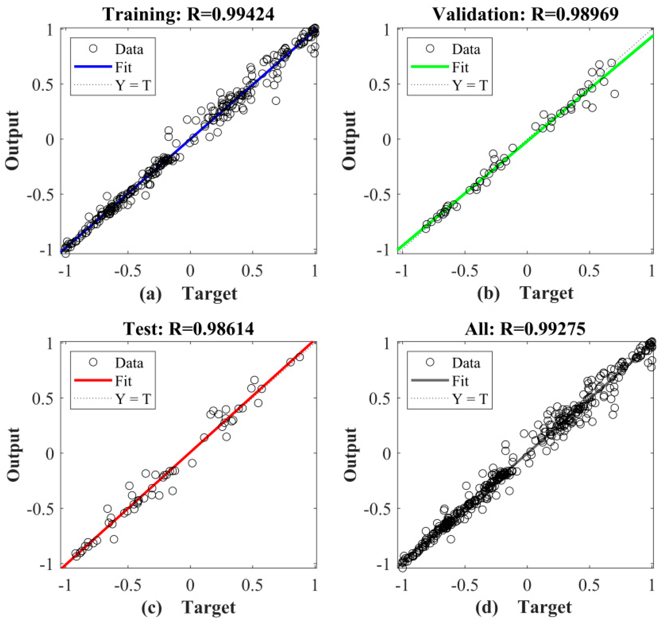
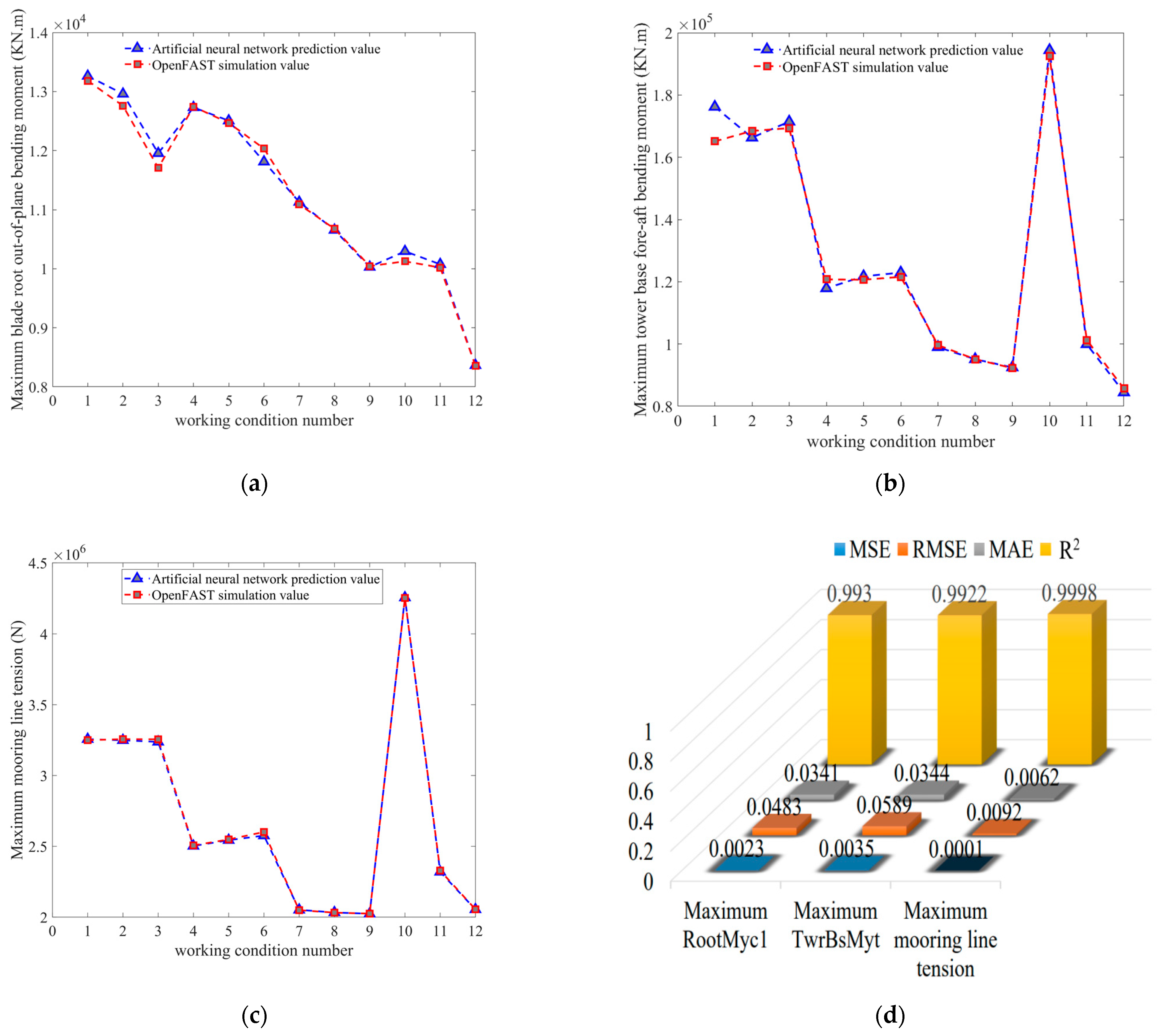
5.2. Reliability of Predictive Models

Extreme sea states will bring more dangers to offshore floating wind turbines in service, and accurate and fast prediction of the dynamic response of FOWT in extreme sea states is crucial to ensuring the safety of floating systems during service. In order to verify the reliability of the trained artificial neural network model, the environmental loading conditions used to verify the reliability of the model were prepared, which are different from the environmental loading conditions used for neural network training; see

Table 7. New environmental parameters for verifying reliability.

${\mathbf{H}}_{\mathbf{S}}\left(\mathbf{m}\right)$	${\mathbf{T}}_{\mathbf{P}}\left(\mathbf{s}\right)$	$\mathbf{W} (\mathbf{m}/\mathbf{s})$	Turbulence Intensity (IEC)	Working Condition Number	Dataset Number
8.31	6	9.80	0.16	1	1
8.31	6	9.80	0.14	2
8.31	6	9.80	0.12	3
8.58	12	10.70	0.16	4	2
8.58	12	10.70	0.14	5
8.58	12	10.70	0.12	6
9.39	24	14.99	0.16	7	3
9.39	24	14.99	0.14	8
9.39	24	14.99	0.12	9
10.17	6	24.2	0.16	10	4
10.17	12	24.2	0.14	11
10.17	24	24.2	0.12	12

. A total of 12 environmental loading conditions used to validate the reliability of the model were categorized into four datasets. Data sets 1, 2, and 3 have different spectral peak periods, which represent the short, medium, and long wavelengths of the ocean environment, and the three conditions in each data set have the same meaningful wave height, spectral peak period, wind speed, and different turbulence intensities. For dataset 4, which represents the extreme ocean environment, the wind speed is close to the cut-out speed of the NREL 5MW wind turbine, and the dataset takes into account both different spectral peak periods and turbulence intensities.

The environmental load conditions used to verify the reliability of the model are substituted into the trained artificial neural network model, and the predicted values of the maximum blade root out-of-plane bending moment, the maximum tower base fore-aft bending moment, and the maximum mooring line tension are obtained. The comparison between the predicted values of the artificial neural network and the OpenFAST simulation values is shown in Figure 15a–c. Data sets 1, 2, and 3 have the same meaningful wave height, spectral peak period, and wind speed. But the turbulence intensity is different. From Figure 15a, it can be seen that the effect of turbulence intensity on the maximum blade root out-of-plane bending moment is obvious, and the larger the turbulence intensity, the larger the maximum blade root out-of-plane bending moment. For data set 4, the average wind speed of the data set is close to the cut-out wind speed of 25 m/s. For the safety of FOWT, the control system will automatically adjust the pitch angle to reduce the blade root out-of-plane bending moment. As shown in Figure 14a, although the wind speed of conditions 10 to 12 is larger than that of conditions 1 to 9, the blade root out-of-plane bending moment is decreasing. It can be seen that the trained neural network model successfully predicts the variation of load with wind speed.

The MSE, RMSE, MAE, and R² of the artificial neural network prediction value and the OpenFAST simulation value are shown in Figure 15d. The MSE, RMSE, and MAE of the maximum mooring line tension are lower than the MSE, RMSE, and MAE of the maximum blade root out-of-plane bending moment of the blade root and the maximum tower base fore-aft bending moment, and the R² of the maximum mooring line tension is higher than the R² of the maximum blade root out-of-plane bending moment of the blade root and the maximum tower base fore-aft bending moment. Smaller MSE, RMSE, and MAE represent higher accuracy. Conversely, a larger R² represents higher accuracy. Therefore, among the three output responses, the prediction accuracy of the maximum mooring line tension is significantly higher than that of the maximum blade root out-of-plane bending moment and the maximum tower base fore-aft bending moment.

Using OpenFAST simulation to obtain the extreme response for 12 operating conditions takes 12 × 630 s. If the proposed artificial neural network prediction model is used, it takes 45 s (Laptop system: Windows 10 home, processor: Intel (R) Core (TM) i7-7500U CPU @ 2.70 GHz 2.90 GHz). The 99.4% time reduction and 167-fold efficiency improvement compared to the OpenFAST simulation demonstrate the computational efficiency advantages of this extreme response prediction model.

6. Summary and Conclusions

The experimental physical quantities (EPQs) that can be obtained are very limited. Therefore, there is a practical concern for designers and industry to obtain accurate non-EPQs. Traditional theoretical and experimental approaches to studying FOWT extreme response statistics are often costly (i.e., model testing) or require time-consuming computational methods.

In order to accelerate FOWT reliability assessment, this study suggests the application of artificial neural networks. Marine environmental data from the TRL+ National Research Project (Spain) was used. The training process of the artificial neural network is highly dependent on the input data, and the number and accuracy of the input data directly affect the training results. Therefore, a large amount of training data was obtained by processing the marine environmental data of the TRL + National Research Project (Spain) through IFORM. TurbSim numerical tool was used to generate turbulent winds as an input to the OpenFAST (Releases v3.5.0) software tool.

The above data were normalized and used for the training of the neural network. The training is completed, and the artificial neural network model is validated, tested, and evaluated by four statistical features. In addition, a sensitivity analysis was performed to show the effect of different numbers of neurons and different numbers of validation checks on the performance of different artificial neural network models. Finally, the new dataset was used to validate the reliability of the proposed neural network extreme response prediction model.

Conclusions drawn through numerical simulation and analysis are as follows:

(1)

Application of IFORM to assess response for data-selected design cases of the TRL + National Research Project can significantly reduce simulation time.

(2)

Neuron sensitivity analysis has shown that deep neural networks with double hidden layers yield better predictions, compared to shallow neural networks with single hidden layers, however further increases in neuron numbers lead to a gradual decrease in model performance.

(3)

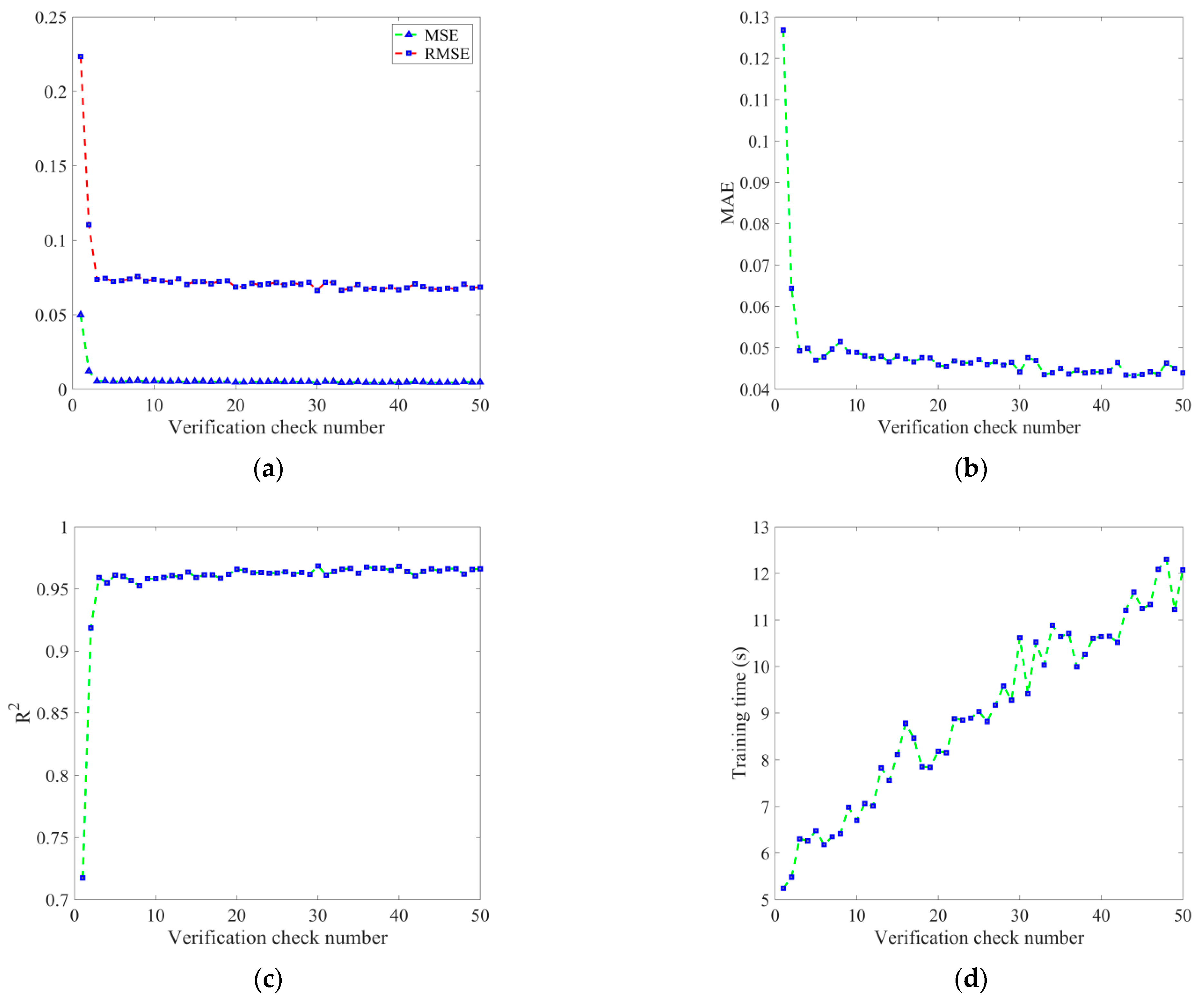
The sensitivity analysis of the number of validations shows that setting too few validations when training the neural network will lead to larger MSE, RMSE, MAE, and smaller R², which indicates that the accuracy of the model is not high. However, too many verifications will take more time, and the improvement in accuracy is almost negligible.

(4)

Reliability verification has shown that a reasonable neural network, as well as appropriate parameter settings of the neural network given in situ wind conditions, may become a useful design strategy.

(5)

Blade element momentum theory, applied to key FOWT parts, wave kinematics, and hydrodynamics calculations, forms a solid mechanical model. Finally, given all the above-mentioned steps, an accurate extreme response statistic for FOWT key parts was obtained.

The developed neural network model is based on marine environment data from bimep (Biscay Marine Energy Platform), so it is not applicable to other wind farms. Each wind farm has a unique marine environment, and therefore, the neural network model needs to be designed for different wind farms. However, there is no need to develop separate grids for individual wind or sea conditions for a single wind farm, as all conditions can be included in the training of the neural network in the early stages, and in fact, the more types of data that are available, the more accurate the predictions will be. For developing a neural network model for a new wind farm, the biggest cost comes from the acquisition of environmental data for the wind farm.

Combining the TRL+ project, the inverse first-order reliability method, and machine learning is a new technical attempt. Future work could consider combining AI with the FOWT digital twin, which requires accurate and instantaneous display and monitoring of engineering structures in the real environment. The technique of combining the digital model of the wind turbine with the actual operating data of the wind turbine to achieve real-time output of the wind turbine loads can provide effective information to wind turbine researchers and developers to reduce the cost of wind turbine design, increase the means of wind turbine control, and optimize the wind turbine operation process. The neural network prediction model proposed in this paper has high accuracy, comparable to the OpenFAST simulation results, and is also fast, which can realize the instant calculation of the FOWT system response and the over-warning of the dangerous state, so as to take measures in advance to guarantee the operational safety of the FOWT system.

References

1. Chen, P.; Jia, C.; Ng, C.; Hu, Z. Application of SADA method on full-scale measurement data for dynamic responses prediction of Hywind floating wind turbines. Ocean Eng. 2021, 239, 109814. [Google Scholar] [CrossRef]
2. Wang, K.; Chu, Y.; Huang, S.; Liu, Y. Preliminary design and dynamic analysis of constant tension mooring system on a 15 MW semi-submersible wind turbine for extreme conditions in shallow water. Ocean Eng. 2023, 283, 115089. [Google Scholar] [CrossRef]
3. Luo, Y.; Qian, F.; Sun, H.; Wang, X.; Chen, A.; Zuo, L. Rigid-flexible coupling multi-body dynamics modeling of a semi-submersible floating offshore wind turbine. Ocean Eng. 2023, 281, 114648. [Google Scholar] [CrossRef]
4. Xu, B.; Kang, H.; Shen, X.; Li, Z.; Cai, X.; Hu, Z. Aerodynamic analysis of a downwind offshore floating wind turbine with rotor uptilt angles in platform pitching motion. Ocean Eng. 2023, 281, 114951. [Google Scholar] [CrossRef]
5. Chen, L.; Basu, B.; Nielsen, S.R.K. A coupled finite difference mooring dynamics model for floating offshore wind turbine analysis. Ocean Eng. 2018, 162, 304–315. [Google Scholar] [CrossRef]
6. Stetco, A.; Dinmohammadi, F.; Zhao, X.; Robu, V.; Flynn, D.; Barnes, M.; Keane, J.; Nenadic, G. Machine learning methods for wind turbine condition monitoring: A review. Renew. Energy 2019, 133, 620–635. [Google Scholar] [CrossRef]
7. International Electrotechnical Commission. IEC 61400-3 Wind Turbines Part 3: Design Requirements for Offshore Wind Turbines; International Electrotechnical Commission: Geneva, Switzerland, 2009. [Google Scholar]
8. Soares, C.G.; Moan, T. Model uncertainty in the long-term distribution of wave-induced bending moments for fatigue design of ship structures. Mar. Struct. 1991, 4, 295–315. [Google Scholar] [CrossRef]
9. Teixeira, A.P.; Soares, C.G. Reliability analysis of a tanker subjected to combined sea states. Probabilistic Eng. Mech. 2009, 24, 493–503. [Google Scholar] [CrossRef]
10. Karmakar, D.; Bagbanci, H.; Soares, C.G. Long-Term Extreme Load Prediction of Spar and Semisubmersible Floating Wind Turbines Using the Environmental Contour Method. J. Offshore Mech. Arct. Eng. 2016, 138, 021601. [Google Scholar] [CrossRef]
11. Soares, C.G.; Garbatov, Y.; Teixeira, A. Methods of structural reliability applied to design and maintenance planning of ship hulls and floating platforms. In Safety and Reliability of Industrial Products, Systems and Structures; Soares, C.G., Ed.; Taylor & Francis Group: London, UK, 2010; pp. 191–206. [Google Scholar]
12. Low, Y.M.; Langley, R.S. A hybrid time/frequency domain approach for efficient coupled analysis of vessel/mooring/riser dynamics. Ocean Eng. 2008, 35, 433–446. [Google Scholar] [CrossRef]
13. Du, J.; Wang, H.; Wang, S.; Song, X.; Wang, J.; Chang, A. Fatigue damage assessment of mooring lines under the effect of wave climate change and marine corrosion. Ocean Eng. 2020, 206, 107303. [Google Scholar] [CrossRef]
14. Low, Y.M.; Cheung, S.H. On the long-term fatigue assessment of mooring and riser systems. Ocean Eng. 2012, 53, 60–71. [Google Scholar] [CrossRef]
15. Chao, S.; Wei, S.; Vahid, J. A real-time hybrid simulation framework for floating offshore wind turbines. Ocean Eng. 2022, 265, 112529. [Google Scholar]
16. Chen, M.; Li, C.B.; Han, Z.; Lee, J.-B. A simulation technique for monitoring the real-time stress responses of various mooring configurations for offshore floating wind turbines. Ocean Eng. 2023, 278, 114366. [Google Scholar] [CrossRef]
17. Jiang, C.; Cao, F.; Li, D.; Wei, Z.; Shi, H. A double-objective prediction and optimization method for buoys performance based on the artificial neural network. Ocean Eng. 2023, 282, 114969. [Google Scholar] [CrossRef]
18. Wang, L.; Zuo, S.; Song, Y.D.; Zhou, Z. Variable Torque Control of Offshore Wind Turbine on Spar Floating Platform Using Advanced RBF Neural Network. Abstr. Appl. Anal. 2014, 2014, 903493. [Google Scholar] [CrossRef]
19. Ahmad, I.; M′zouhi, F.; Aboutalebi, P.; Garrido, I.; Gsrrido, A.J. Fuzzy logic control of an artificial neural network-based floating offshore wind turbine model integrated with four oscillating water columns. Ocean Eng. 2023, 269, 113578. [Google Scholar] [CrossRef]
20. Zifei, X.; Musa, B.; Yang, Y.; Xinyu, W.; Jin, W.; Nduka, E.; Chun, L. Multisensory collaborative damage diagnosis of a 10 MW floating offshore wind turbine tendons using multi-scale convolutional neural network with attention mechanism. Renew. Energy 2022, 199, 21–34. [Google Scholar]
21. Bjørni, F.A.; Lien, S.; Midtgarden, T.A.; Kulia, G.; Verma, A.; Jiang, Z. Prediction of dynamic mooring responses of a floating wind turbine using an artificial neural network. IOP Conf. Ser. Mater. Sci. Eng. 2021, 1201, 012023. [Google Scholar] [CrossRef]
22. Bassam, A.M.; Phillips, A.B.; Turnock, S.R.; Wilson, P.A. Artificial neural network based prediction of ship speed under operating conditions for operational optimization. Ocean Eng. 2023, 278, 114613. [Google Scholar] [CrossRef]
23. Ehrich, S.; Schwarz, C.M.; Rahimi, H.; Stoevesandt, B.; Peinke, J. Comparison of the blade element momentum theory with computational fluid dynamics for wind turbine simulations in turbulent inflow. Appl. Sci. 2018, 8, 2513. [Google Scholar] [CrossRef]
24. Jonkman, J.M.; Hayman, G.; Jonkman, B.; Damiani, R.; Murray, R. AeroDyn v15 User’s Guide and Theory Manual; National Renewable Energy Lab. (NREL): Golden, CO, USA, 2015; p. 46. [Google Scholar]
25. Moriarty, P.J.; Hansen, A.C. AeroDyn Theory Manual. National Renewable Energy Laboratory: Golden, CO, USA, 2005. [Google Scholar]
26. Hansen, M. Aerodynamics of Wind Turbines; Routledge: London, UK, 2015. [Google Scholar]
27. Wood, D. Small wind turbines. In Advances in Wind Energy Conversion Technology; Springer: Berlin/Heidelberg, Germany, 2011; pp. 195–211. [Google Scholar]
28. Tian, W.; Wang, Y.; Shi, W.; Michailides, C.; Wan, L.; Chen, M. Numerical study of hydrodynamic responses for a combined concept of semisubmersible wind turbine and different layouts of a wave energy converter. Ocean Eng. 2023, 272, 113824. [Google Scholar] [CrossRef]
29. Meng, Q.; Hua, X.; Chen, C.; Zhou, S.; Liu, F.; Chen, Z. Analytical study on the aerodynamic and hydrodynamic damping of the platform in an operating spar-type floating offshore wind turbine. Renew. Energy 2022, 198, 772–788. [Google Scholar] [CrossRef]
30. Jonkman, J.M.; Robertson, A.; Hayman, G.J. HydroDyn User’s Guide and Theory Manual; National Renewable Energy Laboratory: Oak Ridge, TN, USA, 2014. [Google Scholar]
31. Jiang, X.; Gan, J.; Teng, S. Simulation of Anchor Chain based on Lumped Mass Method. Theor. Appl. Mech. Lett. 2023, 13, 100460. [Google Scholar] [CrossRef]
32. Hall, M. MoorDyn User’s Guide; Department of Mechanical Engineering, University of Maine: Orono, ME, USA, 2015; p. 15. [Google Scholar]
33. Hall, M.; Goupee, A. Validation of a lumped-mass mooring line model with DeepCwind semisubmersible model test data. Ocean Eng. 2015, 104, 590–603. [Google Scholar] [CrossRef]
34. Barrera, C.; Losada, I.J.; Guanche, R.; Johanning, L. The influence of wave parameter definition over floating wind platform mooring systems under severe sea states. Ocean Eng. 2019, 172, 105–126. [Google Scholar] [CrossRef]
35. Robertson, A.; Jonkman, J.; Masciola, M.; Song, H.; Goupee, A.; Coulling, A.; Luan, C. Definition of the Semisubmersible Floating System for Phase II of OC4. In Scitech Connect Definition of the Floating System for Phase IV of OC3; National Renewable Energy Lab.(NREL): Golden, CO, USA, 2014. [Google Scholar]
36. Liu, Y.; Yoshida, S.; Yamamoto, H.; Toyofuku, A.; He, G.; Yang, S. Response Characteristics of the DeepCwind Floating Wind Turbine Moored by a Single-Point Mooring System. Appl. Sci. 2018, 8, 2306. [Google Scholar] [CrossRef]
37. Iturrioz, A.; del Jesus, F.; Guanche, R.; Acevedo, A.; Chiri, H.; Abascal, A.; García, A.; Espejo, A.; Losada, I.; Marina, D. Metocean characterization of BiMEP for WEC design. In Proceedings of the Twelfth European Wave and Tidal Energy Conference, Cork, UK, 27 August–1 September 2017; pp. 754–759. [Google Scholar]
38. Met-Ocean Conditions for the BIMEP Marine Renewable Energy Test Site. Available online: https://marine.copernicus.eu/services/use-cases/met-ocean-conditions-bimep-marine-renewable-energy-test-site (accessed on 28 April 2023).
39. Haver, S.; Winterstein, S.R. Environmental Contour Lines: A Method for Estimating Long Term Extremes by a Short Term Analysis. Trans.-Soc. Nav. Archit. Mar. Eng. 2008, 116. [Google Scholar]
40. Raed, K.; Teixeira, A.P.; Soares, C.G. Uncertainty assessment for the extreme hydrodynamic responses of a wind turbine semi-submersible platform using different environmental contour approaches. Ocean Eng. 2020, 195, 106719. [Google Scholar] [CrossRef]
41. DNV-OS-J101–Design of Offshore Wind Turbine Structures; DNV GL: Høvik, Norway, 2014.
42. Darin, M.; Sandi, B.Š.; Ivan, L.; Zlatan, C. Prediction of main particulars of container ships using artificial intelligence algorithms. Ocean Eng. 2022, 265, 112571. [Google Scholar]
43. International Electrotechnical Commission. Wind Turbines-Part 1: Design Requirements; IEC 61400-1-Ed. 3.0; International Electrotechnical Commission: Geneva, Switzerland, 2005. [Google Scholar]
44. NREL. OpenFAST Documentation; National Renewable Energy Lab. (NREL): Golden, CO, USA, 2023. [Google Scholar]
45. Jonkman, B. Turbsim User’s Guide v2. 00.00; National Renewable Energy Lab. (NREL): Golden, CO, USA, 2014. [Google Scholar]
46. Li, C.B.; Choung, J.; Noh, M.-H. Wide-banded fatigue damage evaluation of Catenary mooring lines using various Artificial Neural Networks models. Mar. Struct. 2018, 60, 186–200. [Google Scholar] [CrossRef]
47. Ahmadi, F.; Ranji, A.R.; Nowruzi, H. Ultimate strength prediction of corroded plates with center-longitudinal crack using FEM and ANN. Ocean Eng. 2020, 206, 107281. [Google Scholar] [CrossRef]
48. Kanghyeok, L.; Minwoong, C.; Seungjun, K.; Hyoung, S.D. Damage detection of catenary mooring line based on recurrent neural networks. Ocean Eng. 2021, 227, 108898. [Google Scholar]
49. Gorostidi, N.; Nava, V.; Aristondo, A.; Pardo, D. Predictive Maintenance of Floating Offshore Wind Turbine Mooring Lines using Deep Neural Networks. J. Phys. Conf. Ser. 2022, 2257, 012008. [Google Scholar] [CrossRef]
50. Brester, C.; Kallio-Myers, V.; Lindfors, A.V.; Kolehmainen, M.; Niska, H. Evaluating neural network models in site-specific solar PV forecasting using numerical weather prediction data and weather observations. Renew. Energy 2023, 207, 266–274. [Google Scholar] [CrossRef]
51. Han, Y.; Liao, Y.; Ma, X.; Guo, X.; Li, C.; Liu, X. Analysis and prediction of the penetration of renewable energy in power systems using artificial neural network. Renew. Energy 2023, 215, 118914. [Google Scholar] [CrossRef]
52. R2019b, M. MATLAB User Manual; The MathWorks, Inc.: Natick, MA, USA, 2019.
53. Heny, P.; Perdana, W.A.; Restu, A.R.; Susi, S.; Kanti, R.L.; Yuni, F.; Agustiena, M.; Riyana, R.I. Sigmoid Activation Function in Selecting the Best Model of Artificial Neural Networks. J. Phys. Conf. Ser. 2020, 1471, 012010. [Google Scholar]
54. Soyer, M.A.; Tüzün, N.; Karakaş, Ö.; Berto, F. An investigation of artificial neural network structure and its effects on the estimation of the low-cycle fatigue parameters of various steels. Fatigue Fract. Eng. Mater. Struct. 2023, 46, 2929–2948. [Google Scholar] [CrossRef]
55. Li, Z.; Li, Y. A comparative study on the prediction of the BP artificial neural network model and the ARIMA model in the incidence of AIDS. BMC Med. Inform. Decis. Mak. 2020, 20, 143. [Google Scholar] [CrossRef]
56. Cheng, K.; Tao, F.; Zhan, Y.; Li, M.; Li, K. Hierarchical attributes learning for pedestrian re-identification via parallel stochastic gradient descent combined with momentum correction and adaptive learning rate. Neural Comput. Appl. 2019, 32, 5695–5712. [Google Scholar] [CrossRef]
57. Banibrata, P.; Bhaskar, K. Heart disease prediction using scaled conjugate gradient backpropagation of artificial neural network. Soft Comput. 2022, 27, 6687–6702. [Google Scholar]
58. Kayri, M.; Pakdemirli, M. Predictive Abilities of Bayesian Regularization and Levenberg–Marquardt Algorithms in Artificial Neural Networks: A Comparative Empirical Study on Social Data. Math. Comput. Appl. 2016, 21, 20. [Google Scholar] [CrossRef]
59. Kazemi, P.; Renka, R.J. A Levenberg–Marquardt method based on Sobolev gradients. Nonlinear Anal. 2012, 75, 6170–6179. [Google Scholar] [CrossRef]
Figure 1. Flow angles and local element velocities [25].
Jmse 11 01807 g001
Figure 2. Local elemental forces [25].
Jmse 11 01807 g002
Figure 3. Schematic diagram of a lumped mass method [32].
Jmse 11 01807 g003
Figure 4. NREL 5 MW semi-submersible floating offshore wind turbine with OC4 DeepCwind Semi-submersible platform [34].
Jmse 11 01807 g004
Figure 5. TRL+ National research project [37,38]. (a) Location and dimensions of bimep test site; (b) WAVESCAN buoy installed in bimep.
Jmse 11 01807 g005
Figure 6. Marine Environment of Different Return Periods. (a) IFORM results of the significant wave height HS and wind speed W; (b) IFORM results of the HS and peak wave period TP (right) for the BiMEP area [34].
Jmse 11 01807 g006
Figure 7. FOWT dynamics modeling based on OpenFAST, blade root out-of-plane bending moment (RootMyc1), tower base fore-aft bending moment (TwrBsMyt).
Jmse 11 01807 g007
Figure 8. Dynamic response for condition 1, A (blade root out-of-plane bending moment), B (tower base fore-aft bending moment), C (mooring line tension).
Jmse 11 01807 g008
Figure 9. Artificial neural network topology, RootMyc1 (blade root out-of-plane bending moment), TwrBsMyt (tower base fore-aft bending moment).
Jmse 11 01807 g009
Figure 10. ANN-based forecasting modeling framework, RootMyc1 (blade root out-of-plane bending moment), TwrBsMyt (tower base fore-aft bending moment).
Jmse 11 01807 g010
Figure 11. Flowchart for determining the optimal network structure with four implicit layers.
Jmse 11 01807 g011
Figure 12. Comparison of Forecast Model Output and Expectations.
Jmse 11 01807 g012
Figure 13. Performance indicators of neural networks. (a) Mean squared error; (b) Root mean square error; (c) Mean absolute error; (d) Coefficient of determination.
Jmse 11 01807 g013
Figure 14. Impact of the number of validations during neural network training on performance metrics. (a) Mean squared error and Root mean square error; (b) Mean absolute error; (c) Coefficient of determination; (d) Training time.
Jmse 11 01807 g014
Figure 15. Verify the reliability of the model, RootMyc1 (blade root out-of-plane bending moment), TwrBsMyt (tower base fore-aft bending moment). (a) Maximum blade root out-of-plane bending moment; (b) Maximum tower base fore-aft bending moment; (c) Maximum mooring line tension; (d) Performance indicators.
Jmse 11 01807 g015