Abstract
This work presents a new model for surf and swash zone morphology evolution induced by nonlinear waves. Wave transformation in the surf and swash zones is computed by a nonlinear wave model based on the higher order Boussinesq equations for breaking and non-breaking waves. Regarding sediment transport, the model builds on previous research by the authors and incorporates the latest update of a well-founded sediment transport formula. The wave and morphology evolution model is validated against two sets of experiments on beach profile change and is afterwards used to test the performance of a widely-adopted erosion/accretion criterion. The innovation of this work is the validation of a new Boussinesq-type morphology model under both erosive and accretive conditions at the foreshore (accretion is rarely examined in similar studies), which the model reproduces very well without modification of the empirical coefficients of the sediment transport formula used; furthermore, the model confirms the empirical erosion/accretion criterion even for conditions beyond the ones it was developed for and without imposing any model constraints. The presented set of applications highlights model capabilities in simulating swash morphodynamics, as well as its suitability for coastal erosion mitigation and beach restoration design
1. Introduction
Coastal erosion is nowadays among the most intensively investigated topics in coastal research. This is justified by the expected impact of climate change on the intensity of the drivers behind it (both natural- and human- induced; [1,2,3,4,5,6]), as well as on its direct association to the inundation of low-lying areas [7,8,9,10]. Since building coastal resilience against erosion and flooding is based on the effective design of coastal protection and adaptation measures [11,12], numerical models have become indispensable tools for scientists, engineers and policymakers. As such, their accuracy and reliability are continuously tested in both research and engineering applications [13,14,15,16,17,18].
The study of coastal morphology evolution is particularly demanding. Its accurate representation by numerical models depends on the scales in space and time over which the interplay between various codependent processes is to be taken into consideration. General discussion and valuable insights on the topic can be found in [19,20,21,22,23,24,25,26]. Regardless, though, the fundamentals of coastal morphodynamics lie in a beach profile’s response to wave action.
The swash, i.e., the part of the beach where the sediment bed is submerged and alternatively exposed, due to uprush and backwash, plays a key role in coastal morphology evolution through both cross-shore and longshore processes. Regarding longshore transport and its modelling in the swash, useful insights can be found in [15,27,28,29,30,31]. Focusing on cross-shore processes, it is documented that waves acting upon a beach profile which is not in equilibrium will redistribute sediment across it as the beach adjusts towards equilibrium shape. Cross-shore transport will be predominantly directed either onshore or offshore, the former leading to accretion at the foreshore (berm formation) and the latter to erosion at the foreshore with the eroded sediment forming a notable bar near the breaker line (hence the typical distinction between accretive and erosive profiles).
The above processes in the swash can be broken down and modelled through understanding the interplay between swash flow velocities, bed shear stress, bore collapse-induced turbulence, wave-swash interactions, infragravity waves, in-/ex-filtration and pressure gradients (horizontal and vertical). Chen at al. [32] present a thorough review on the dynamics of sand transport in the swash and on the use of practical models to simulate it. Reference is also made to works that delve into the intricacies of swash zone dynamics, like the experimental work of [33,34], the modelling works of [35,36,37] and the combined experimental—numerical works of [38,39]. Modelling attempts in relevant literature are typically based on the reproduction of sets of seminal experiments, like the ones collected and presented by [40]. It is noteworthy, though, that profiles with prominent accretive patterns at the foreshore are scarcely studied compared to erosive ones.
This work presents a new advanced phase-resolving nonlinear wave, sediment transport and bed morphology evolution 2DH model, that builds on previous research by the authors [13] and incorporates the latest update of a well-founded sediment transport formula [41]. The model is validated against two sets of experiments on beach profile change, namely the U.S. Army Corps of Engineers (CE) experiments and the Central Research Institute of Electric Power Industry (CRIEPI) experiments [40], with particular focus on prominent accretive profiles, and is afterwards used to test the performance of a widely-adopted erosion/accretion criterion. Section 2 in the following presents the components and theoretical background of the wave and morphology evolution model. Section 3 presents the characteristics of model applications. Section 4 presents and discusses model results, and Section 5 presents the conclusions drawn from this work, along with insights for future research.
2. The Wave and Morphology Evolution Model
The wave and morphology evolution model used in this work is an improved version of the model presented by [13], with regard to its essential sediment transport module.
The advanced phase-resolving wave model is based on the higher-order Boussinesq-type Equations for breaking and nonbreaking waves, expressed as:
where Mu is defined as:
and G as:
where ζ is the wave surface elevation, d is the water depth and h is the total water depth (h = d + ζ); the subscript “t” denotes differentiation with respect to time; U is the horizontal velocity vector U = (U,V); τb = (τbx, τby) is the bed friction term calculated according to [42,43]; δ is the roller thickness, determined geometrically according to [44]; E is the eddy viscosity term, calculated according to [45]; and uo is the bottom velocity vector uo = (uo, vo), with uo and vo being the instantaneous bottom velocities along the x- and y- directions respectively. Following [43], wave breaking is initiated using breaking angle φb = 30°, which then gradually changes to its terminal value φb =10°.
The model is capable of simulating the phenomena of shoaling, refraction, breaking, diffraction, reflection and wave-structure interaction, as well as nonlinear wave-wave interaction. Regarding model capabilities in simulating the non-linear evolution of unidirectional or multidirectional wave fields in the nearshore, one can refer to [46] (see also [47] on the issue). Regarding wave-structure interaction and energy transmission, one can refer to [48]. The model is analysed in detail in [13] and description is not repeated here. The model’s implementation to diverse coastal engineering applications can be found in [16,43,49].
Regarding the sediment transport module, this work builds on the improvements introduced by [13] and adopts the latest update of the transport formula of [50,51] proposed by [41]. Bed load and sheet flow transport is accordingly simulated using [41]:
where:
In Equations (5)–(9): aw and b are empirical coefficients (set to 6 and 4.5, respectively); fw is the wave friction factor; Φm is the friction angle for a moving grain (set to 30 deg); d50 is the median grain size; dx is the local bottom slope; de is the depth (for equilibrium conditions); θcw,m and θcw are the mean and maximum Shields parameters due to wave-current interaction, respectively; and θcr is the critical Shields parameter for incipient motion of the sediment. It is noted that c and t are indices that refer to the wave crest and wave through, respectively, with peak velocities u to be perceived accordingly and û calculated following the approach of [52]. Both the phase-lag and acceleration effects are introduced in the calculation of θcw,net that is used for the derivation of Equation (5), as in [50,51].
Suspended load and bed morphology evolution are simulated as in [13], based on the combined formulation of [50,51,53,54] and the equation of [55], respectively. Regarding the connection to the nonlinear wave model, specifically, it is noted that breaking wave-induced turbulence and the generated undertow (as a return flow due to surface roller effects of broken waves) lead to offshore-directed suspended load. On the other hand, under non-breaking waves or under relatively weak breaking/undertow conditions the time-averaged bed load and sheet flow transport (Equation (5)) is usually directed onshore, due to near-bottom velocity asymmetry together with the acceleration effects. The difference of the two quantities (i.e., the total load), along with runup/backwash flow effects, determine the direction of the total sediment transport rate and consequently dictate the erosion/accretion process.
The methodology adopted for the series of model applications can be encoded into the steps also described in [13], and is repeated in the following for reasons of completeness. First, the initial bathymetry is inserted into the wave model in order to estimate the wave and current fields. These fields are afterwards used by the sediment transport module to calculate the sediment transport rates. Finally, bathymetry is updated by the sediment transport module solving the equation of the conservation of sediment transport [55] for the transport rates calculated in the previous step. The procedure is repeated for a user-specified time period or until a state of morphologic equilibrium is reached.
3. Model Applications
3.1. Validation for Experimental Data
Two sets of experiments are used in this work for the validation of the wave and morphology evolution model: The US Army Corps of Engineers experiments and the Central Research Institute of Electric Power Industry experiments [40], referred to as CE and CRIEPI experiments in the following, respectively.
The CE experiments were conducted in 1956/1957 and 1962 in the 221.0 m long, 5.2 m wide and 7.0 m deep Large Wave Tank of the US Army Corps of Engineers Beach Erosion Board (henceforth referred to as LWT). The LWT was at the time of the experiments located at Dalecarlia (Washington DC, US; see [56] for facility details). The full dataset comprises two series of movable-bed model experiments on beach profile change, mainly distinguished by the grain size of the bed material used. Tests of monochromatic waves of varying steepness were run for the different grain sizes in order to produce either accreting or eroding profiles. Nineteen (19) cases are documented in [40,56]: all but two started from a plane slope of 1:15; water depths (at the flat section of the flume) ranged from 3.5 m to 4.6 m; grain sizes with median diameters of 0.22 mm and 0.40 mm were used; wave heights ranged between 0.55 m and 1.68 m; wave periods ranged between 3.75 s and 16.0 s. Tests were continued until the establishment of stable beach profiles in all runs (i.e., until no significant profile changes were detected). This work focuses on tests that resulted in prominent erosive and—most importantly—accretive profiles at the foreshore; these are Tests no. 300 and 301 from the CE experiments. The specific tests conditions are presented in Table 1, in which d50 is the median grain size, H is the wave height, T is the wave period, d is the water depth and Dur is Test duration.

Table 1.
Test conditions for the CE and CRIEPI experiments reproduced in this work (eros. = erosive test; accr. = accretive test).
The CRIEPI experiments were conducted between 1979 and 1983 in the 205.0 m long, 3.4 m wide and 6.0 m deep Large Wave Flume of the Central Research Institute of Electric Power Industry in Japan (see [57,58] for facility details). Similar to the CE experiments, tests of monochromatic waves of varying steepness were run for different grain sizes in order to produce either accreting or eroding profiles. Twenty four (24) cases are documented in [40,57,58]: initial plane slope varied between 1:50 and 1:10, although for some tests the profile from the previous test was used as initial profile; water depths (at the flat section of the flume) ranged from 3.5 m to 4.5 m; grain sizes with median diameters of 0.27 mm and 0.47 mm were used; wave heights ranged between 0.30 m and 1.80 m; wave periods ranged between 3.0 s and 12.0 s. As mentioned in the previous, this work focuses on tests that resulted in prominent erosive and—most importantly—accretive profiles at the foreshore; these are Tests no. 3-1 and 1-3 from the CRIEPI experiments, whose conditions are also presented in Table 1.
3.2. Investigation of an Erosion/Accretion Criterion
Criteria for distinguishing profile response under wave action have always been of interest in relevant research, as their utility extends from practical reasons (e.g., quickly estimating the expected profile response for large datasets) to enriching our understanding of the interplay between wave conditions and profile characteristics (profile shape and sediment properties) that leads to sediment redistribution patterns in the surf zone and in the swash.
In the process of developing and presenting the profile evolution model SBEACH, Larson and Kraus [59] present previous research on criteria for identifying profile response (e.g., [60,61,62,63,64,65]) and eventually propose the criterion expressed as:
where Ho, Lo is the deep water wave height and wavelength, respectively, w is the sediment fall speed and M is an empirical parameter set to 0.0007 for regular waves in the lab or mean wave height in the field. The criterion implies predominant sediment transport offshore that leads to erosion at the foreshore for Ho/Lo < 0.0007(Ho/wT)3, and predominant sediment transport onshore that leads to accretion at the foreshore for Ho/Lo > 0.0007(Ho/wT)3. The respective profiles are typically referred to as “erosive/bar” or “accretive/berm” profiles, since erosion at the foreshore leads to the formation of a prominent bar near the breaker line and accretion at the foreshore leads to berm buildup. These two types of profiles are also referred to as winter-summer, storm-normal or dissipative-reflective profiles in literature. The criterion of [59], formally presented in [66,67], has been established as the most widely used since, although variations of its formulation have also been proposed and discussed in future research by [68,69,70,71,72,73,74,75], based on the same or different experimental datasets.
This work focuses on expanding the set of conditions tested during the CE and CRIEPI experiments (see Section 3.1 and [40,56,57,58]), using the wave and morphology evolution model presented Section 2 and validated in Section 3.1. This is done in order to investigate the performance of the Larson and Kraus criterion in predicting erosive/bar and accretive/berm profiles. A total of 22 New Tests were run, with the set of combinations of wave conditions and profile characteristics used in each one presented in Table 2 (slope for all runs was set equal to 1:20; New Tests are henceforth denoted as NT).
Table 2.
Test conditions for the investigation of the erosion/accretion criterion of Larson and Kraus [59] (NT = New Test; slope for all runs equal to 1:20).
4. Results and Discussion
4.1. Results for Model Validation
Figure 1 presents results for Test 300 from the CE experiments (see Table 1). Figure 1a shows the comparison of the measured and computed (by the model) profiles (including model results for t = Dur/2), Figure 1b shows the difference between measured and computed profiles, and Figure 1c shows the net sediment transport rate (positive values = onshore transport, negative values = offshore transport). Figure 2, Figure 3 and Figure 4 present the respective results for Test 301 from the CE experiments and Tests 3-1, 1-3 from the CRIEPI experiments (also see Table 1). For the accretive tests CE 300 and CRIEPI 3-1 the Equilibrium Beach Profiles (EBPs) according to [76] are also presented in Figure 1a and Figure 3a, respectively; so are the differences between measured and EBPs/Dean profiles in Figure 1b and Figure 3b. Equilibrium Beach Profiles follow equation d = Ay2/3, where d is the depth, y is the cross-shore distance measured from the shoreline and A is a parameter associated to the median grain size according to [77].
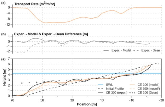
Figure 1.
Results for Test CE 300 (see Table 1): (a) comparison of measured and computed profiles (* denotes model results at t = Dur/2) and respective Dean EBP; (b) difference between measured and computed/Dean profiles; (c) computed net sediment transport rate (positive values = onshore transport, negative values = offshore transport).

Figure 2.
Results for Test CE 301 (see Table 1): (a) comparison of measured and computed profiles (* denotes model results at t = Dur/2); (b) difference between measured and computed profiles; (c) computed net sediment transport rate (positive values = onshore transport, negative values = offshore transport).
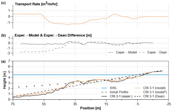
Figure 3.
Results for Test CRIEPI 3-1 (see Table 1): (a) comparison of measured and computed profiles (* denotes model results at t = Dur/2) and respective Dean EBP; (b) difference between measured and computed/Dean profiles; (c) computed net sediment transport rate (positive values = onshore transport, negative values = offshore transport).
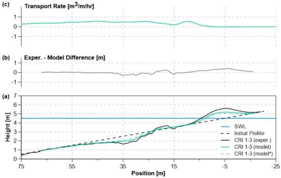
Figure 4.
Results for Test CRIEPI 1-3 (see Table 1): (a) comparison of measured and computed profiles (* denotes model results at t = Dur/2); (b) difference between measured and computed profiles; (c) computed net sediment transport rate (positive values = onshore transport, negative values = offshore transport).
Model results compare very well with the experimental data, overall. Regarding the erosive tests (i.e., Tests CE 300—Figure 1 and CRIEPI 3-1—Figure 3) the model simulates accurately the loss of sediment from the shoreface and the gradual formation of the longshore bar, as well as the erosion-accretion transitions along the profile, in both cases. Model results for the computed profiles at half the Tests’ durations (denoted as “Model*” in Figure 1 and Figure 3) are indicative of the evolution of erosive profiles as simulated by the presented model. Between Tests, results are comparatively better for Test CRIEPI 3-1; however, absolute differences between measured and computed profiles are significantly below 0.5 m for both Tests and exceed this value only locally. The mean, variance and standard deviation of said absolute differences are calculated to be equal to 0.22 m, 0.032 m and 0.17 m, respectively, for Test CE 300, and equal to 0.14 m, 0.009 m and 0.09 m, respectively, for Test CRIEPI 3-1.
On the other hand, the EBPs according to [76] (denoted as “Dean” in Figure 1 and Figure 3) do not simulate profile evolution with comparable accuracy, especially seaward of the erosion-accretion transitions. Absolute differences between measured and EBPs/Dean profiles exceed 1 m along large parts of the profiles. The mean, variance and standard deviation of said absolute differences are calculated to be equal to 0.49 m, 0.52 m and 0.72 m, respectively, for Test CE 300, and equal to 0.75 m, 0.48 m and 0.69 m, respectively, for Test CRIEPI 3-1.
Regarding the—more significant in the context of this work—accretive tests (i.e., Test CE 301—Figure 2 and CRIEPI 1-3—Figure 4), the model simulates accurately the accumulation of sediment at the foreshore and the gradual formation of the berm, in both cases. The significance of the specific feat should be particularly acknowledged, especially considering the size of the berm, in terms of both shoreline advance at SWL and accreted volume. Morphology evolution in the subaerial parts of the profiles is captured satisfactorily, although there appears to be a relative weakness in capturing erosion-accretion transitions underwater that needs to be further investigated. Model results for the computed profiles at half the Tests’ durations (denoted as “Model*” in Figure 2 and Figure 4) are indicative of the evolution of accretive profiles as simulated by the presented model. Absolute differences between measured and computed profiles are significantly below 0.4 m for both Tests and approach this value only locally. The mean, variance and standard deviation of said absolute differences are calculated to be equal to 0.20 m, 0.021 m and 0.14 m, respectively, for Test CE 301, and equal to 0.13 m, 0.013 m and 0.11 m, respectively, for Test CRIEPI 1-3.
It is important to highlight that the wave and morphology evolution model presented in this work achieved the results of Figure 1, Figure 2, Figure 3 and Figure 4 without any modification of the empirical coefficients of the transport formula of Equation (5). The values of these coefficients were set to aw = 6 and b = 4.5 in all model runs, exactly as proposed by Zhang and Larson [41].
4.2. Results for the Investigation of an Erosion/Accretion Criterion
Table 3 presents results for the test conditions presented in Table 2 (NT = New Test). It is noted that Erosion (E) and Accretion (A) classifications in Table 3 refer to model results regarding the equilibrium profile at the end of each simulation. After calculating the respective Ho/wT and Ho/Lo sets of values, results are also presented in Figure 5, along with all data for CE and CRIEPI experiments presented in [40].
Table 3.
Model results for the test conditions presented in Table 2 (NT = New Test). Erosion (E) and Accretion (A) classifications refer to model results regarding the equilibrium profile at the end of each simulation.
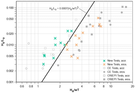
Figure 5.
Profile response with regard to accretion (accr.) or erosion (eros.) as simulated by the wave and morphology evolution model of this work for the New Test conditions of Table 2 (see also Table 3), along with the observations in the CE and CRIEPI experiments [40]. The solid line represents the limit of the Larson and Kraus criterion [59], i.e., Ho/Lo = 0.0007(Ho/wT)3.
Figure 5 shows that the wave and morphology evolution model’s results and the Larson and Kraus criterion agree in predicting erosive/bar and accretive/berm profiles for a wide range of test conditions, even beyond the CE/CRIEPI experiments regarding both wave conditions and profile characteristics. It is noted again, as for the validation tests of Section 3.1 and Section 4.1, that all model runs were setup without modifying the empirical coefficients of the transport formula of Equation (5) from the values sets by Zhang and Larson [41].
5. Conclusions
The new wave and morphology evolution model presented and used in this work builds on previous research by the authors and adopts a new formula for the calculation of sediment transport. Model applications were designed in order to, first, validate the model against experimental data (with particular focus on prominent accretive profiles which are rarely examined in relevant research), and then use it to test the performance of one of the best-known erosion/accretion criteria. The results presented in Section 4 are deemed to highlight the innovative aspects of this work, namely: (a) the accurate simulation of accretive conditions at the foreshore (with a particular note on the relative magnitude of the phenomenon in the selected tests); (b) the fact that the model reproduces experimental data very well for both accretive and erosive profiles with no modification of the empirical coefficients in the sediment transport formula proposed by Zhang and Larson [41]; and (c) the confirmation of the empirical criterion of Larson and Kraus [59] even for conditions beyond the ones it was developed for, without imposing any model constraints.
This work is deemed to provide useful insights on the modelling of morphology evolution in the swash for both research and engineering applications. Along with complementary authors’ work on the integrated modelling of coastal wave dynamics, hydrodynamics and morphodynamics [13,15,16,20,77], it is furthermore considered as a step towards research on the combination of advanced numerical models and machine learning methods in coastal engineering.
Author Contributions
Conceptualization, methodology, model development, model validation, model applications, formal analysis, visualization, writing, A.G.S. and T.V.K. All authors have read and agreed to the published version of the manuscript.
Funding
This research received no external funding.
Institutional Review Board Statement
Not applicable.
Informed Consent Statement
Not applicable.
Data Availability Statement
Data is contained within the article.
Conflicts of Interest
The authors declare no conflict of interest.
References
- Gao, W.; Liu, J.; Xu, Y.; Li, P. Evolution of sandy shores under the combined impact of global climate change and anthropogenic activities in Shandong Peninsula, East China. J. Asian Earth Sci. 2024, 259, 105887. [Google Scholar] [CrossRef]
- Leal, K.B.; Robaina, L.E.d.S.; De Lima, A.d.S. Coastal impacts of storm surges on a changing climate: A global bibliometric analysis. Nat. Hazards 2022, 114, 1455–1476. [Google Scholar] [CrossRef]
- Lobeto, H.; Menendez, M.; Losada, I.J. Future behavior of wind wave extremes due to climate change. Sci. Rep. 2021, 11, 7869. [Google Scholar] [CrossRef] [PubMed]
- Flor-Blanco, G.; Alcántara-Carrió, J.; Jackson, D.W.T.; Flor, G.; Flores-Soriano, C. Coastal erosion in NW Spain: Recent patterns under extreme storm wave events. Geomorphology 2021, 387, 107767. [Google Scholar] [CrossRef]
- Toimil, A.; Camus, P.; Losada, I.J.; Le Cozannet, G.; Nicholls, R.J.; Idier, D.; Maspataud, A. Climate change-driven coastal erosion modelling in temperate sandy beaches: Methods and uncertainty treatment. Earth Sci. Rev. 2020, 202, 103110. [Google Scholar] [CrossRef]
- Mentaschi, L.; Vousdoukas, M.I.; Voukouvalas, E.; Dosio, A.; Feyen, L. Global changes of extreme coastal wave energy fluxes triggered by intensified teleconnection patterns. Geophys. Res. Lett. 2017, 44, 2416–2426. [Google Scholar] [CrossRef]
- Kirezci, E.; Young, I.R.; Ranasinghe, R.; Muis, S.; Nicholls, R.J.; Lincke, D.; Hinkel, J. Projections of global-scale extreme sea levels and resulting episodic coastal flooding over the 21st Century. Sci. Rep. 2020, 10, 11629. [Google Scholar] [CrossRef]
- Han, X.; Kuang, C.; Zhu, L.; Gong, L.; Cong, X. Hydrodynamical and morphological patterns of a sandy coast with a beach nourishment suffering from a storm surge. Coast Eng. J. 2022, 64, 83–99. [Google Scholar] [CrossRef]
- Cueto, J.E.; Otero Díaz, L.J.; Ospino-Ortiz, S.R.; Torres-Freyermuth, A. The role of morphodynamics in predicting coastal flooding from storms on a dissipative beach with sea level rise conditions. Nat. Hazards Earth Syst. Sci. 2022, 22, 713–728. [Google Scholar] [CrossRef]
- Postacchini, M.; Melito, L.; Ludeno, G. Nearshore Observations and Modeling: Synergy for Coastal Flooding Prediction. J. Mar. Sci. Eng. 2023, 11, 1504. [Google Scholar] [CrossRef]
- IPCC. Climate Change 2022: Impacts, Adaptation and Vulnerability; Contribution of Working Group II to the Sixth Assessment Report of the Intergovernmental Panel on Climate Change; IPCC: Cambridge, UK; New York, NY, USA, 2022; p. 3056. [Google Scholar]
- IPCC. Climate Change 2022: Mitigation of Climate Change; Working Group III Contribution to the Sixth Assessment Report of the Intergovernmental Panel on Climate Change; IPCC: Cambridge, UK; New York, NY, USA, 2022; p. 1991. [Google Scholar]
- Karambas, T.V.; Samaras, A.G. Soft shore protection methods: The use of advanced numerical models in the evaluation of beach nourishment. Ocean Eng. 2014, 92, 129–136. [Google Scholar] [CrossRef]
- Postacchini, M.; Russo, A.; Carniel, S.; Brocchini, M. Assessing the Hydro-Morphodynamic Response of a Beach Protected by Detached, Impermeable, Submerged Breakwaters: A Numerical Approach. J. Coast. Res. 2016, 32, 590–602. [Google Scholar]
- Karambas, T.V.; Samaras, A.G. An Integrated Numerical Model for the Design of Coastal Protection Structures. J. Mar. Sci. Eng. 2017, 5, 50. [Google Scholar] [CrossRef]
- Samaras, A.G.; Karambas, T.V. Modelling the Impact of Climate Change on Coastal Flooding: Implications for Coastal Structures Design. J. Mar. Sci. Eng. 2021, 9, 1008. [Google Scholar] [CrossRef]
- Mohapatra, S.C.; Fonseca, R.; Guedes Soares, C. A comparison between analytical and numerical simulations of solutions of the coupled Boussinesq equations. In Maritime Technology and Engineering 3; Guedes Soares, C., Santos, T.A., Eds.; Taylor & Francis Group: Abingdon, UK, 2016; pp. 1175–1180. [Google Scholar]
- Mohapatra, S.C.; Guedes Soares, C. Shallow water hydrodynamics: Comparing solutions of the coupled Boussinesq equations in shallow water. In Maritime Technology and Engineering; Guedes Soares, C., Santos, T.A., Eds.; CRC Press: Boca Raton, FL, USA, 2014; p. 8. [Google Scholar]
- Anthony, E.J. Wave influence in the construction, shaping and destruction of river deltas: A review. Mar. Geol. 2015, 361, 53–78. [Google Scholar] [CrossRef]
- Samaras, A.G. Towards integrated modelling of Watershed-Coast System morphodynamics in a changing climate: A critical review and the path forward. Sci. Total Environ. 2023, 882, 163625. [Google Scholar] [CrossRef]
- French, J.; Payo, A.; Murray, B.; Orford, J.; Eliot, M.; Cowell, P. Appropriate complexity for the prediction of coastal and estuarine geomorphic behaviour at decadal to centennial scales. Geomorphology 2016, 256, 3–16. [Google Scholar] [CrossRef]
- Nicholls, R.J.; French, J.R.; van Maanen, B. Simulating decadal coastal morphodynamics. Geomorphology 2016, 256, 1–2. [Google Scholar] [CrossRef]
- Van Maanen, B.; Nicholls, R.J.; French, J.R.; Barkwith, A.; Bonaldo, D.; Burningham, H.; Brad Murray, A.; Payo, A.; Sutherland, J.; Thornhill, G.; et al. Simulating mesoscale coastal evolution for decadal coastal management: A new framework integrating multiple, complementary modelling approaches. Geomorphology 2016, 256, 68–80. [Google Scholar] [CrossRef]
- Zhou, Z.; Coco, G.; Townend, I.; Olabarrieta, M.; van der Wegen, M.; Gong, Z.; D’Alpaos, A.; Gao, S.; Jaffe, B.E.; Gelfenbaum, G.; et al. Is “Morphodynamic Equilibrium” an oxymoron? Earth-Sci. Rev. 2017, 165, 257–267. [Google Scholar] [CrossRef]
- Ranasinghe, R. On the need for a new generation of coastal change models for the 21st century. Sci. Rep. 2020, 10, 2010. [Google Scholar] [CrossRef] [PubMed]
- Bayındır, C.; Farazande, S. The solution of the long-wave equation for various nonlinear depth and breadth profiles in the power-law form. Dyn. Atmos. Ocean. 2021, 96, 101254. [Google Scholar] [CrossRef]
- Jiang, A.W.; Hughes, M.; Cowell, P.; Gordon, A.; Savioli, J.C.; Ranasinghe, R. A hybrid model of swash-zone longshore sediment transport on reflective beaches. In Proceedings of the 32nd International Conference on Coastal Engineering, Shanghai, China, 30 June–5 July 2010. [Google Scholar] [CrossRef]
- Kamphuis, J.W. Alongshore sediment transport rate. J. Waterw. Port Coast. Ocean. Eng. 1991, 117, 624–640. [Google Scholar] [CrossRef]
- Kamphuis, J.W. Alongshore Transport Rate of Sand. In Proceedings of the 28th International Conference on Coastal Engineering, Cardiff, Wales, 7–12 July 2002; World Scientific: Wales, UK, 2003; pp. 2478–2490. [Google Scholar]
- Larson, M.; Wamsley, T.V. A Formula for Longshore Sediment Transport in the Swash. In Coastal Sediments ’07; ASCE Library: Reston, VA, USA, 2007; pp. 1924–1937. [Google Scholar]
- Samaras, A.G.; Karambas, T.V. On the simulation of longshore sediment transport in the swash zone in linear wave models. In Proceedings of the 7th IAHR Europe Congress, Athens, Greece, 7–9 September 2022; pp. 112–113. [Google Scholar]
- Chen, W.; van der Werf, J.J.; Hulscher, S.J.M.H. A review of practical models of sand transport in the swash zone. Earth-Sci. Rev. 2023, 238, 104355. [Google Scholar] [CrossRef]
- Deng, B.; Zhang, W.; Tang, H.S.; Jiang, C.B.; Liu, X.J. An experimental study on hydrodynamic process, beach profile, and sand migration in swash zone under action of dam-break bore. Appl. Ocean Res. 2022, 129, 103391. [Google Scholar] [CrossRef]
- Pontiki, M.; Puleo, J.A.; Bond, H.; Wengrove, M.; Feagin, R.A.; Hsu, T.J.; Huff, T. Geomorphic Response of a Coastal Berm to Storm Surge and the Importance of Sheet Flow Dynamics. J. Geophys. Res. F Earth Surf. 2023, 128, e2022JF006948. [Google Scholar] [CrossRef]
- Briganti, R.; Torres-Freyermuth, A.; Baldock, T.E.; Brocchini, M.; Dodd, N.; Hsu, T.J.; Jiang, Z.; Kim, Y.; Pintado-Patiño, J.C.; Postacchini, M. Advances in numerical modelling of swash zone dynamics. Coast. Eng. 2016, 115, 26–41. [Google Scholar] [CrossRef]
- Postacchini, M.; Othman, I.K.; Brocchini, M.; Baldock, T.E. Sediment transport and morphodynamics generated by a dam-break swash uprush: Coupled vs uncoupled modeling. Coast. Eng. 2014, 89, 99–105. [Google Scholar] [CrossRef]
- Tazaki, T.; Harada, E.; Gotoh, H. Numerical investigation of sediment transport mechanism under breaking waves by DEM-MPS coupling scheme. Coast. Eng. 2022, 175, 104146. [Google Scholar] [CrossRef]
- Pinault, J.; Morichon, D.; Delpey, M.; Roeber, V. Field observations and numerical modeling of swash motions at an engineered embayed beach under moderate to energetic conditions. Estuarine Coast. Shelf. Sci. 2022, 279, 108143. [Google Scholar] [CrossRef]
- Spyrou, D.; Karambas, T.V. Experimental and numerical simulation of cross-shore morphological processes in a nourished beach. J. Coast. Res. 2021, 37, 1012–1024. [Google Scholar] [CrossRef]
- Dette, H.H.; Larson, M.; Murphy, J.; Newe, J.; Peters, K.; Reniers, A.; Steetzel, H. Application of prototype flume tests for beach nourishment assessment. Coast. Eng. 2002, 47, 137–177. [Google Scholar] [CrossRef]
- Zhang, J.; Larson, M. A Numerical Model for Offshore Mound Evolution. J. Mar. Sci. Eng. 2020, 8, 160. [Google Scholar] [CrossRef]
- Kobayashi, N.; Agarwal, A.; Johnson, B.D. Longshore current and sediment transport on beaches. J. Water Port Coast. Ocean. Eng. 2007, 133, 296–304. [Google Scholar] [CrossRef]
- Karambas, T.V.; Karathanassi, E.K. Longshore sediment transport by nonlinear waves and currents. J. Water Port Coast. Ocean. Eng. 2004, 130, 277–286. [Google Scholar] [CrossRef]
- Schäffer, H.A.; Madsen, P.A.; Deigaard, R. A Boussinesq model for waves breaking in shallow water. Coast. Eng. 1993, 20, 185–202. [Google Scholar] [CrossRef]
- Chen, Q.; Dalrymple, R.A.; Kirby, J.T.; Kennedy, A.B.; Haller, M.C. Boussinesq modeling of a rip current system. J. Geophys. Res. Oceans 1999, 104, 20617–20637. [Google Scholar] [CrossRef]
- Memos, C.D.; Karambas, T.V.; Avgeris, I. Irregular wave transformation in the nearshore zone: Experimental investigations and comparison with a higher order Boussinesq model. Ocean Eng. 2005, 32, 1465–1485. [Google Scholar] [CrossRef]
- Polnikov, V.G.; Manenti, S. Study of Relative Roles of Nonlinearity and Depth Refraction in Wave Spectrum Evolution in Shallow Water. Eng. Appl. Comput. Fluid Mech. 2009, 3, 42–55. [Google Scholar] [CrossRef][Green Version]
- Kriezi, E.; Karambas, T. Modelling wave deformation due to submerged breakwaters. Proc. Inst. Civ. Eng. Marit. Eng. 2010, 163, 19–29. [Google Scholar] [CrossRef]
- Samaras, A.G.; Karambas, T.V.; Archetti, R. Simulation of tsunami generation, propagation and coastal inundation in the Eastern Mediterranean. Ocean Sci. 2015, 11, 643–655. [Google Scholar] [CrossRef]
- Camenen, B.; Larson, M. A Unified Sediment Transport Formulation for Coastal Inlet Application; ERDC/CH: CR-07-1; US Army Corps of Engineers, Engineering Research and Development Center: Vicksburg, MS, USA, 2007; p. 247. [Google Scholar]
- Camenen, B.; Larson, M. A general formula for noncohesive suspended sediment transport. J. Coast. Res. 2008, 24, 615–627. [Google Scholar] [CrossRef]
- Grasmeijer, B.T.; Ruessink, B.G. Modeling of waves and currents in the nearshore parametric vs. probabilistic approach. Coast. Eng. 2003, 49, 185–207. [Google Scholar] [CrossRef]
- Karambas, T.V. Prediction of sediment transport in the swash-zone by using a nonlinear wave model. Cont. Shelf Res. 2006, 26, 599–609. [Google Scholar] [CrossRef]
- Karambas, T.V.; Koutitas, C. Surf and swash zone morphology evolution induced by nonlinear waves. J. Water Port Coast. Ocean. Eng. 2002, 128, 102–113. [Google Scholar] [CrossRef]
- Leont’yev, I.O. Numerical modelling of beach erosion during storm event. Coast. Eng. 1996, 29, 187–200. [Google Scholar] [CrossRef]
- Kraus, N.C.; Larson, M. Beach Profile Change Measured in the Tank for Large Waves 1956–1957 and 1962; Techical Report CERC-88-6; US Army Corps of Engineers: Washington, DC, USA, 1988; p. 167. [Google Scholar]
- Kajima, R.; Saito, S.; Shimizu, T.; Maruyama, K.; Hasegawa, H.; Sakakiyama, T. Sand Transport Experiments Performed by Using a Large Water Wave Tank; Central Research Institute of Electric Power Industry, Civil Engineering Division: Abiko, Japan, 1983. [Google Scholar]
- Kajima, R.; Shimizu, T.; Maruyama, K.; Saito, S. Experiments on beach profile change with a large wave flume. Coast. Eng. Proc. 1982, 1, 85. [Google Scholar] [CrossRef]
- Larson, M.; Kraus, N.C. SBEACH. Numerical Model for Simulating Storm-Induced Beach Change; Report 1: Empirical Foundation and Model Development; Technical Report CERC-89-9; USACE Waterways Experiment Station: Vicksburg, MS, USA, 1989. [Google Scholar]
- Dean, R.G. Heuristic Models of Sand Transport in the Surf Zone. In Proceedings of the Conference on Engineering Dynamics in tle Surf Zone, Sydney, Australia, 14–17 May 1973; pp. 208–214. [Google Scholar]
- Kriebel, D.L.; Dally, W.R.; Dean, R.G. Undistorted Froude Model for Surf Zone Sediment Transport. In Proceedings of the 20th International Conference on Coastal Engineering, Taipei, Taiwan, 9–14 November 1987; pp. 1296–1310. [Google Scholar]
- Sunamuza, T.; Horikawa, K. Two-Dimensional Beach Transformation Due to Waves. In Proceedings of the 14th International Conference on Coastal Engineering, Copenhagen, Denmark, 24–28 June 1975; pp. 920–938. [Google Scholar]
- Sunamura, T. Parameters for Delimiting Erosion and Accretion of Natural Beaches; Annual Report of the Institute of Geoscience, Report No. 6; University of Tsukuba: Tsukuba, Japan, 1980; pp. 51–54. [Google Scholar]
- Hattori, M.; Kawamata, R. Onshore-Offshore Transport and Beach Profile Change. In Proceedings of the 17th International Conference on Coastal Engineering, Sydney, Australia, 23–28 March 1980; pp. 1175–1193. [Google Scholar]
- Wright, L.D.; Short, A.D. Morphodynamic Variability of Surf Zones and Beaches: A Synthesis. Mar. Geol. 1984, 56, 93–118. [Google Scholar] [CrossRef]
- Larson, M.; Kraus, N.C. Numerical model of longshore current for bar and trough beaches. J. Water Port Coast. Ocean. Eng. 1991, 117, 326–347. [Google Scholar] [CrossRef]
- Larson, M.; Kraus, N.C. Mathematical modeling of the fate of beach fill. Coast. Eng. 1991, 16, 83–114. [Google Scholar] [CrossRef]
- Ahrens, J.P.; Hands, E.B. Parameterizing Beach Erosion/Accretion Conditions. In Proceedings of the 26th International Conference on Coastal Engineering, Copenhagen, Denmark, 22–26 June 1998; Volume 1. [Google Scholar]
- Dalrymple, R.A. Prediction of Storm/Normal Beach Profiles. J. Water Port Coast. Ocean. Eng. 1992, 118, 193–200. [Google Scholar] [CrossRef]
- Dalrymple, R.A. Closure to “Prediction of Storm/Normal Beach Profiles” by Robert A. Dalrymple (March/April, 1992, Vol. 118, No. 2). J. Water Port Coast. Ocean. Eng. 1993, 119, 473–474. [Google Scholar] [CrossRef]
- Jiménez, J.A.; Sánchez-Arcilla, A. Simulación de cambios a corto plazo en la línea de costa. Rev. Obras Públicas 1992, 3315, 41–51. [Google Scholar]
- Jiménez, J.A.; Sánchez-Arcilla, A.; Stive, M.J.F. Discussion of “Prediction of Storm/Normal Beach Profiles” by Robert A. Dalrymple (March/April, 1992, Vol. 118, No. 2). J. Water Port Coast. Ocean. Eng. 1993, 119, 466–468. [Google Scholar] [CrossRef]
- Kraus, N.C.; Mason, J.M. Discussion of “Prediction of Storm/Normal Beach Profiles” by Robert A. Dalrymple (March/April, 1992, Vol. 118, No. 2). J. Water Port Coast. Ocean. Eng. 1993, 119, 468–470. [Google Scholar] [CrossRef]
- Seymour, R.J.; Riedl, S.J. Discussion of “Prediction of Storm/Normal Beach Profiles” by Robert A. Dalrymple (March/April, 1992, Vol. 118, No. 2). J. Water Port Coast. Ocean. Eng. 1993, 119, 471–473. [Google Scholar] [CrossRef]
- Kraus, N.C.; Larson, M.; Kriebel, D.L. Evaluation of beach erosion and accretion predictors. In Coastal Sediments ’91; ASCE Library: Reston, VA, USA, 1991; pp. 572–587. [Google Scholar]
- Dean, R.G. Equilibrium beach profile: Characteristics and applications. J. Coast. Res. 1991, 7, 53–84. [Google Scholar]
- Samaras, A.G.; Iliadis, L.; Karambas, T.V. A methodology for harbour layout design based on Machine Learning. In Proceedings of the 40th IAHR World Congress, Vienna, Austria, 21–23 August 2023. [Google Scholar]


Disclaimer/Publisher’s Note: The statements, opinions and data contained in all publications are solely those of the individual author(s) and contributor(s) and not of MDPI and/or the editor(s). MDPI and/or the editor(s) disclaim responsibility for any injury to people or property resulting from any ideas, methods, instructions or products referred to in the content. |
© 2024 by the authors. Licensee MDPI, Basel, Switzerland. This article is an open access article distributed under the terms and conditions of the Creative Commons Attribution (CC BY) license (https://creativecommons.org/licenses/by/4.0/).