Abstract
The formation of oil–mineral aggregates (OMAs) is essential for understanding the behavior of oil spills in estuaries and coastal waters. We utilized statistical methods (screening design) to identify the most influential variables (seven factors in total) during OMA formation. Time was the most important factor, followed by temperature and oil/clay ratio. Moreover, machine learning was applied to predict the OMA median diameter (D50). Among the three tested algorithms, the Random Forest (RF) algorithm showed the highest accuracy, with a training R2 of 0.99 and testing R2 of 0.93. An open-source software tool that integrates the RF algorithm was developed, allowing users to easily estimate the OMA D50 based on input variables. The valuable results and the practical tool we have developed enhance the understanding and management of environmental impacts associated with oil spills.
1. Introduction
Oil spill incidents persist as one of the most critical contributors to marine environmental pollution [1]. These spills usually have long-term negative impacts on the marine environment and ecology [2]. When an oil spill accident happens in coastal and estuarine waters, the dispersed oil droplets may interact with suspended sediment particles and form oil–mineral aggregates (OMAs) [3,4,5,6,7,8]. In general, the density of oil is lower than that of water, while the density of sediment is higher. Therefore, the density of OMAs may be lower, higher, or equal to that of water, depending on the properties and formation of oil droplets and sediment particles. Hence, the movement of OMAs in the water column can be very different due to relative density to the local water; it may float to the water surface, sink to the bottom, or move with water. The transport of OMAs is important for oil spill modeling [9].
The initial conceptualization of potential interactions between oil and mineral particles in an aqueous medium was proposed by Poirier and Thiel (1941) [7]. They suggested that kaolinite, a type of clay mineral, was particularly effective in promoting oil sedimentation [7]. However, the phenomenon of flocculation between oil and mineral particles in natural environments was not observed until the cleanup operations following the Exxon Valdez oil spill in Prince William Sound, Alaska, in 1989 [10]. The term “clay–oil flocculation” was subsequently used to describe this occurrence [10,11]. Scientists then theorized that this mechanism could facilitate the removal of spilled oil from water columns, even in low-energy environments [3,10,11,12]. This hypothesis was corroborated by subsequent oil spills, including those in Tampa Bay, Florida (1993), and the Sea Empress spill in Wales (1996) [5]. The term “oil–mineral aggregates (OMAs)” was later adopted to describe these interactions, as it became evident that not only clay-sized minerals (<2 µm) contributed to the formation of OMAs [4,13].
The process of OMA formation is a crucial natural mechanism that facilitates oil transportation between environmental compartments, thereby promoting oil dispersion [3,12,13]. Previous studies reported that OMA formation is influenced by a multitude of factors; for example, Gong et al. (2014) suggested that the properties of the oil (e.g., type, droplet size, and concentration), the properties of the mineral particles (e.g., size, shape, density, concentration, and organic matter content), and ambient conditions (e.g., temperature, salinity, and mixing energy) [14]. Despite extensive research into OMA formation under various conditions, the formation mechanisms remain controversial [15]. For example, regarding the impact of salinity on OMA formation, some studies have suggested that low salinity levels (0–5 ppt) have a strong influence, while no significant effect was observed with increasing salinity [16,17,18,19]. However, Guyomarch et al. (1999) reported the opposite result, with increasing salinity from 10 to 50 ppt having a profound effect on OMA formation [20].
It is worthwhile noting that different OMA formation studies employed varying laboratory operations, leading to significant variance and uncertainty in the reported data. Unfortunately, few studies have attempted to replicate experimental runs to quantify experimental error [17,21,22], resulting in less reliable data [23]. The complexity inherent in the OMA formation system is evident [14]. However, there appears to be an absence of systematic research aimed at identifying key influencing factors through statistical design and analysis approaches [15]. The potential for interaction effects between various factors, such as the effect of temperature over time, is an important aspect of the OMA formation process. This is largely unexplored and represents a critical area for further research.
Meanwhile, recent developments in big data processing, enhanced computing capabilities, and machine learning algorithms have significantly impacted scientific research and industrial operations [24,25,26]. Machine learning techniques are gaining prominence across various research domains, including those related to oil spills. For instance, Cao et al. (2022) utilized machine learning to examine the influence of salinity and chemical dispersants on the biodegradation of spilled oil. They quantitatively predicted the strength of the relationship among dispersant use, salinity, cell count, and other variables [24]. Given the capacity of machine learning to process extensive datasets and its predictive accuracy, there is growing interest in its application in forecasting OMA formation, which we focus on in the present study.
The objective of this investigation is to study the formation of OMA under various conditions, identify the significant factors and interaction effects, and assess the potential for using machine learning algorithms to predict OMA formation. Based on the study by Gong et al. (2014) [14], in this study, seven factors, namely salinity, temperature, time, oil/clay ratio, agitation speed, clay type, and the presence/absence of dispersants were selected for evaluation, and the median OMA diameter was used as the response variable. The influence of varying periods affects oil droplet dynamics, consequently impacting OMA size. The use of dispersants modifies oil viscosity and interfacial tension, influencing OMA stability. Variations in clay concentrations were implemented, along with different salinity levels, to replicate marine and river plume environments and simulate natural turbidity. A screening design statistical approach was adopted to design the experiment and identify the most influential factors and interactions. Furthermore, a dataset was created by integrating data from this study and the existing literature [16,18,27,28,29,30,31,32], which was then utilized to train three machine learning algorithms: Random Forest (RF), Gradient Boosting Regression (GBR), and Adaptive Boost Regression (AdaBoost). The predictive value of each model was evaluated, and the stability and generalizability of the optimal model were assessed. Lastly, an application software was developed to enable the prediction of the median OMA diameter by inputting OMA formation conditions. The findings of this study offer valuable insights into the mechanisms underlying OMA formation, facilitating the development of more accurate models to simulate the fate and transport of spilled oil in estuarine and coastal environments.
2. Materials and Methods
2.1. Materials
In this investigation, crude oil characterized by a density of 799.2 kg/m3 and a viscosity of 61.1 cSt was employed. The mineral components selected were kaolinite and montmorillonite; both are readily available in various natural environments, including soils and sediments. Their widespread availability and cost-effectiveness make them suitable for oil spill remediation through OMA formation [33]. Depending on the experimental conditions, kaolinite (2788.9 kg/m3 of density) or montmorillonite (2172.5 kg/m3 of density) was utilized. Additionally, a chemical dispersant, JAFIRST™001 (Xinluo Industrial Co., Ltd., Shanghai, China), was applied at a dispersant-to-oil ratio (DOR) of 1:10, adhering to the predefined experimental parameters. Previous studies have indicated that this specific DOR ratio enhances OMA formation [34].
2.2. OMA Formation Experiments
The experimental design was implemented using the Screening Design feature in Minitab 19 software, with the level settings detailed in Table 1. A temperature of 0 °C was selected to simulate the winter conditions in most coastal areas. Temperatures of 15 °C and 30 °C were chosen to represent summer conditions in various coastal environments globally. The former is characteristic of temperate coastal regions, including Northern Europe, southern Australia, and the northeastern United States [35]. The latter represents tropical and subtropical areas, such as the Gulf of Mexico, the Caribbean, northern Australia, and Southeast Asia [35]. Regarding salinity, 0 ppt was used to simulate river water, while 17 ppt was selected to represent coastal regions influenced by riverine input or estuarine conditions. A salinity of 34 ppt was chosen to simulate subtropical and tropical coastal waters. Previous studies have shown that mixing durations of 4 and 6 h effectively form OMAs, thus these durations were used [30,36,37], along with an 8-h interval to examine the impact of extended mixing time. Agitation speeds of 100, 130, and 160 revolutions per minute (rpm), corresponding to shear rates of approximately 15, 18, and 20 s−1 [38], were selected based on their demonstrated efficacy in OMA formation in prior research [16,31,36]. Oil-to-clay ratios of 1:2, 1:1, and 2:1, identified as influential in oil trapping efficiency, were also tested [31,39].

Table 1.
Level settings for the seven studied factors for oil–mineral aggregate formation experiments.
Each experimental run was duplicated to minimize experimental errors, with detailed runs provided in Supplementary Materials Table S1. For each experiment, 100 mL of aqueous solution with the desired salinity level was prepared. Then, 40 mg of crude oil and 20–80 mg of clay (depending on clay type and oil/clay ratio) were added to a 250 mL Erlenmeyer flask containing the solution. The sample-containing flask was agitated using a temperature-controllable shaker (see Figure S1 in Supplementary Materials) to form OMAs. Samples were collected hourly, and the OMA structures were analyzed using inverted microscopy (see Figure S2 in Supplementary Materials). The OMA size (area and perimeter) was measured using Image processing software (ImageJ 1.53k.exe).
2.3. Machine Learning Model
The present study employed three tree-based machine learning algorithms, namely RF, GBR, and AdaBoost, to predict the median diameter of OMAs. These algorithms were selected due to their capacity to model the nonlinear relationships between input features and response variables. Additionally, their robustness against outliers and noise in data made them suitable choices for this analysis. A more detailed description of these algorithms is provided in the study by Yu et al. (2023) [26]. The models were developed using Scikit-learn libraries in the Anaconda3 environment based on Python 3.9 [40]. The input dataset was subjected to a nested cross-validation (CV) procedure, wherein the inner and outer loops comprised 5 folds. The outer loop was employed to obtain a less biased estimation of model performance, while the inner loop was used for model tuning, specifically the optimization of hyperparameters. In the hyperparameter tuning stage, a grid-search method was implemented to determine the optimal values of “max_depth” and “n_estimator.” The range for “n_estimator” was set within the 1 to 100 range, incremented by 5, while “max_depth” was evaluated between 5 and 100. After determining optimal hyperparameters, they were integrated into the model’s framework. The specific nested CV procedure is presented in Figure 1. The nested CV procedure was initiated by a random shuffling of the dataset (random state = 40) prior to its division into five equally sized folds. Within each outer loop iteration, a single fold was reserved for the final testing set; the remaining data was subjected to the inner loop. This inner loop was characterized by a 5-fold CV serving the purpose of hyperparameter tuning and model selection. The model’s overall efficacy was determined by computing the mean performance metric across all iterations in the outer loop. Finally, the best estimator was saved and used for further analysis.
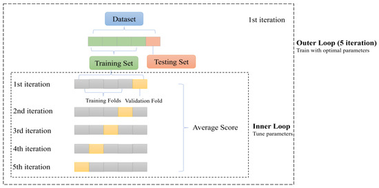
Figure 1.
Nested cross-validation procedure, comprising five iterations in the inner and outer loops.
2.4. Model Evaluation
Assessment of the models’ predictive accuracy was conducted using the coefficient of determination (R2), root means square error (RMSE), and 95% confidence interval (CI) [41]. A model is considered more accurate if it exhibits a higher R2, and lower RMSE and 95% CI values. The calculation of these metrics is based on the following equations:
where denotes the sample size; and denote the predicted and actual values of the sample, respectively; is the mean of the actual values; denotes the standard deviation.
Upon the establishment of models through the nested CV procedure for the three distinct algorithms, the optimal model was selected based on its superior performance, as evidenced by the highest R2, lowest RMSE, and lowest 95% CI. Prior to deploying this selected model, a further evaluation was performed by applying varied test/train splits to examine the stability and generalizability of the model. The proportions of the original dataset assigned to the training set started at 10% and increased by 10% at each iteration, reaching 90% of the original dataset. Simultaneously, the portion of the original dataset allocated to the testing set, initially comprising 90%, was reduced by 10% with each iteration, ultimately constituting only 10% of the original dataset [42,43]. Importantly, to prevent any potential bias or order effects, the dataset underwent a random shuffling procedure (random state = 40) before the division of data. This ensures a randomized allocation of data instances, supporting the reliability and validity of the subsequent model evaluations.
2.5. Machine Learning Quantification of Feature Importance
In this study, two approaches were adopted to assess the significance of each feature. The first approach was the conventional feature importance, involving the calculation of the Gini importance derived from the Gini index. The Gini index served as the metric for assessing the purity of nodes within decision trees, where a higher Gini index corresponded to lower purity. The Gini decrease was quantified as the difference between the totaled Gini indexes of divided nodes and the Gini index of each individual node. The Gini importance, measured on a scale from 0 to 1, was derived by proportionally weighing the Gini decrease relative to the frequency of the node’s occurrence in all trees. A greater Gini importance value indicated a more substantial impact of the factor. This analysis utilized the feature importance tools available in the Scikit-learn libraries.
In addition to the conventional feature importance, permutation feature importance was utilized. This method quantifies the influence of each feature on the model’s performance by measuring the decrease in performance subsequent to a random permutation of the feature’s values. If the model’s performance decreased significantly when a feature’s values were shuffled, the feature was considered important. This measure provided an additional layer of robustness to the evaluation of feature significance, accounting for the impact of each feature on the model’s predictive accuracy.
This study further assessed the influence of each feature on the predictive model using a technique known as partial dependence plots (PDPs). These plots provide a graphical representation of the marginal effect of a feature on the predicted outcome of a machine-learning model, holding all other features constant. This method offers valuable insights into the nature and strength of the relationship between each feature and the predicted outcome, facilitating an understanding of the model’s behavior beyond the insights provided by feature importance metrics alone. By observing how the predictions vary with changes in a feature’s values, potential nonlinearities and interactions with other features can be identified, contributing to a more comprehensive understanding of the model’s inner workings. In this study, for the PDPs, the presence or absence of dispersants was indicated by values 0 or 1 respectively. The other factors utilized 100 values, evenly spaced between the maximum and minimum values.
2.6. Machine Learning-Based Software
This section introduces the machine learning-based software developed for predicting the median diameter of OMAs. The software utilizes machine learning algorithms selected based on their superior performance, characterized by the highest R2 values and lowest RMSE and 95% CI values. The operational workflow of the software comprises three main components:
- Input parameters: The software requires the following input data to perform predictions:
- Time: Duration of the experiment (min)
- Clay type: Density of the clay used (g/cm3)
- Oil type: Density of the oil used (g/cm3)
- Dispersant: A binary input indicating the presence (Yes) or absence (No) of dispersants
- Oil concentration: Concentration of oil in the mixture (mg/L)
- Clay concentration: Concentration of clay in the mixture (mg/L)
- Salinity: Salinity of the mixture (ppt)
- Shaking rate: Agitation speed (rpm)
- Temperature: Ambient temperature during the experiment (°C)
- Process: The software applies the selected machine-learning algorithm to the input data. This algorithm has been optimized for accuracy and reliability in predicting the median diameter of OMAs based on the input parameters.
- Output: The primary output of the software is the predicted median diameter of OMAs (µm). This aids in understanding the behavior of OMAs under different experimental condition.
3. Results and Discussions
3.1. Statistical Analysis
3.1.1. Significance Analysis of the Formation Factors
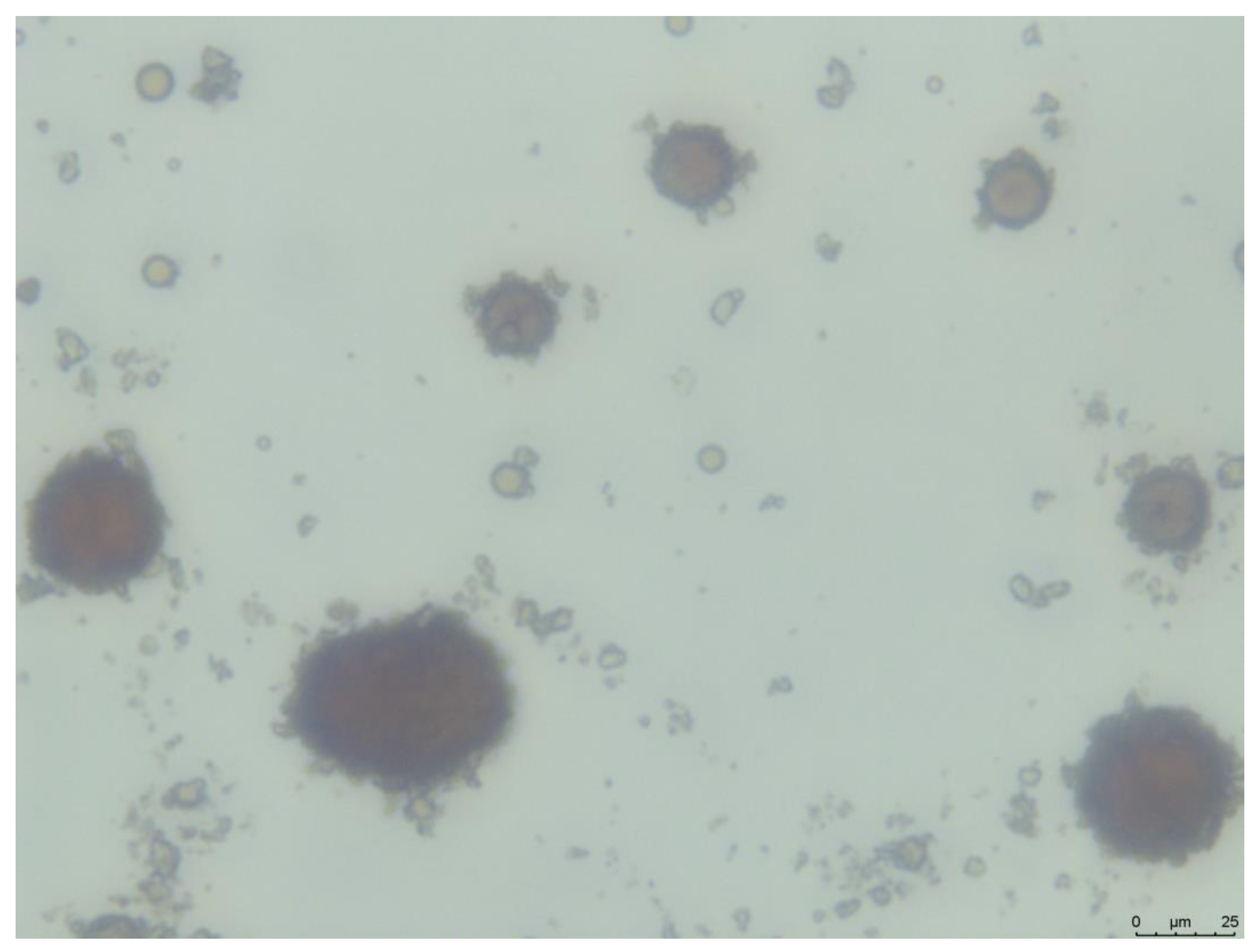
Based on previous studies [16,17,28,30,32,36,39], the formation of OMAs is mainly controlled by temperature, salinity, time, agitation speed, clay type, oil/clay weight ratio, and the presence or absence of dispersants. However, the level of their impact on the median diameter (D50) of OMAs has not been thoroughly investigated and compared. In this study, a statistical method, screening design, was used to estimate the significance of these factors. A representative image of OMAs captured through inverted microscopy is presented in Figure 2, while the detailed experimental design and raw data are available in the Supplementary Materials (Table S1). A paired t-test carried out in Minitab produced a p-value of 0.329, higher than the 0.05 significance level. This implies no significant statistical variance between the means of the OMA D50 in the two experimental setups. Consequently, this analysis suggests that measurement inaccuracies and human errors did not significantly influence the study’s outcomes. Analysis of variance (ANOVA) was employed to assess the impact of various factors on OMA D50, with results summarized in Table 2 and Equation (3). The analysis identified time as the most influential factor on OMA median diameter, as indicated by a p-value significantly less than 0.05 and the highest F-value of 22.48. The temperature and oil/clay ratio were also identified as significant influencers of D50, with p-values of 0.014 and 0.023, respectively. However, the effect of clay type was only marginally significant (0.05 < p-value = 0.069 < 0.1) in affecting D50.
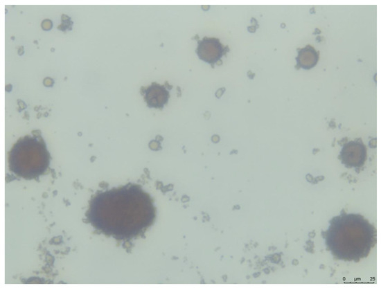
Figure 2.
Example of oil–mineral aggregates (OMAs) acquired through inverted microscopy.
Table 2.
Analysis of variance in the median diameter (D50) of oil-mineral aggregates.
A regression model was developed to capture the relationship between the identified significant factors, involving their interaction effects and response variable (OMA median diameter), as shown in Equation (4). The model coefficients were estimated using the least squares method. The equation is as follows:
where , , , and denote temperature (°C), time (hours), clay type (kaolinite and montmorillonite denoted as −1 and +1, respectively), and oil/clay ratio (1:2, 1:1, and 2:1 denoted as 25, 50, and 75, respectively).
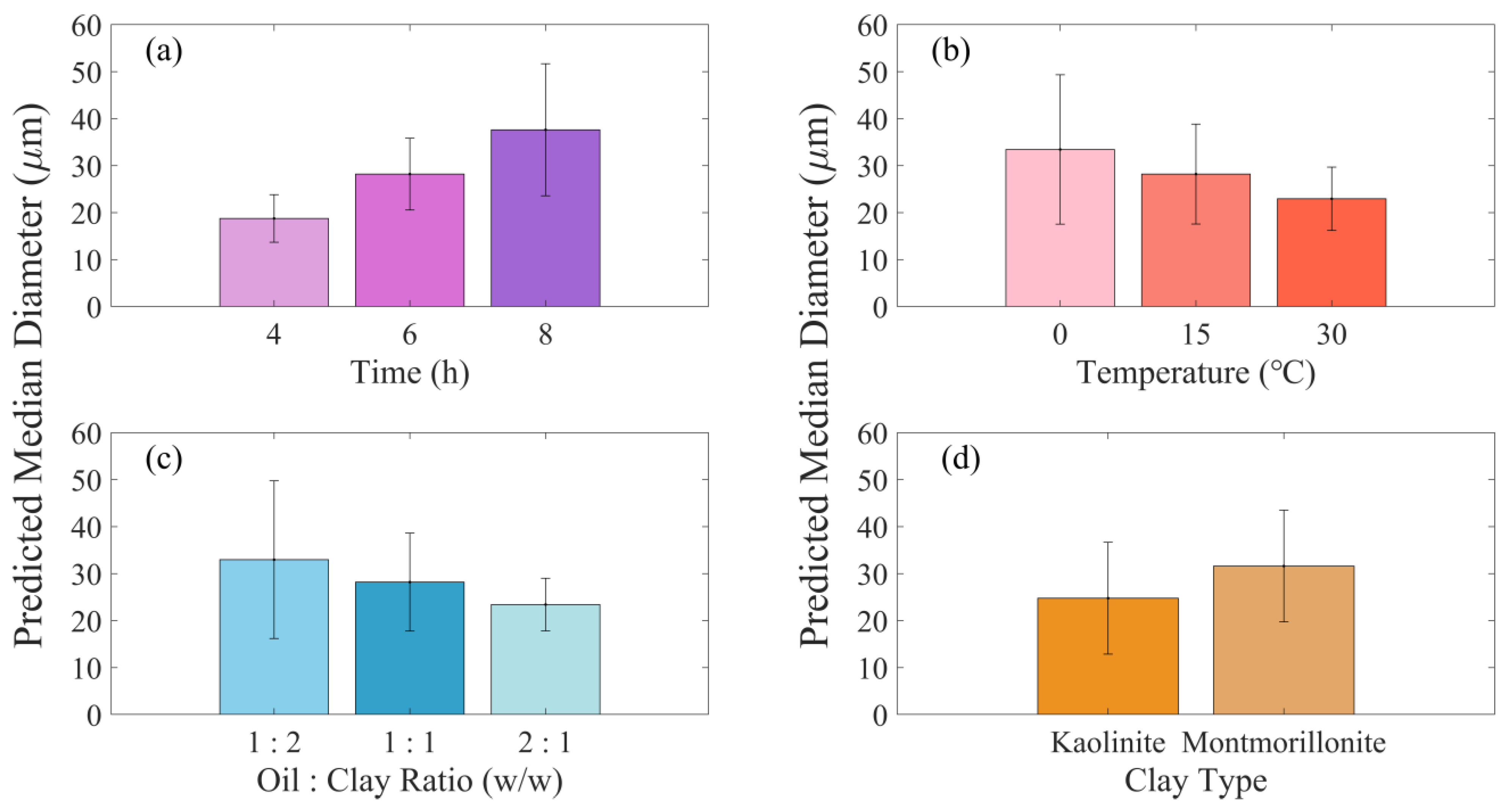
A quantitative analysis of the impact of identified factors (time, temperature, oil/clay ratio, and clay type) on D50 was conducted via Equation (4) and illustrated in Figure 3. Figure 3a demonstrates a direct correlation between extended mixing times and increased D50. It was observed that increasing the duration from 4 to 8 h increased D50 from 19 µm to 38 µm, implying that longer mixing periods promote the formation of larger OMAs. This finding is consistent with previous studies [31,44]. Sun et al. (2014) explored the effect of time on OMA size. They reported an increase with extended duration, potentially due to the incorporation or coalescence of small oil droplets into or onto the OMA structure [31]. In contrast, Ji et al. (2021) noted a decrease in OMA D50 with increasing mixing time, proposing that this could be attributed to the continuous fragmentation of OMAs into smaller aggregates [28]. Additionally, Zhao et al. (2014) discovered that for many light to moderately viscous oils, equilibrium in oil droplet size distribution is usually attained within a relatively short timeframe, often less than several tens of minutes [45]. This finding implies that oil viscosity plays a critical role in determining the final size distribution of OMAs. Beyond viscosity, oil-water interfacial tension presents a more substantial barrier to droplet breakage, as demonstrated by a sharp decline in the breakage rate of oil droplets with increasing interfacial tension [46]. This resistance could significantly impact OMA formation and sizing during extended mixing periods. These opposing findings, along with the influence of oil’s physical properties, underscore the complexity of the factors affecting OMA formation. This emphasizes the necessity for further research to reveal the precise impact of mixing time on OMA formation.
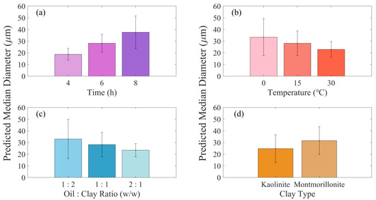
Figure 3.
Impact of significant factors (a) time, (b) temperature, (c) oil/clay ratio, and (d) clay type on the median diameter of oil-mineral aggregates.
The impact of temperature on OMA D50 is presented in Figure 3b. The findings suggest that increasing the temperature from 0 °C to 30 °C leads to a gradual reduction in OMA D50, indicating that higher temperature conditions favor the formation of smaller OMAs. This observed phenomenon can be linked to the reduction in oil viscosity as temperature rises, which consequently facilitates the dispersion of oil into small droplets [47]. Additionally, the increase in temperature typically leads to a decrease in oil–water surface tension, further promoting the formation and dispersion of smaller oil droplets [48]. This simultaneous decrease in viscosity and surface tension at higher temperatures plays a crucial role in enhancing the dispersibility and spread of oil in aqueous environments. As a result, the OMA D50 exhibits a decline in correspondence with increasing temperature.
Increasing the oil/clay ratio from 1:2 to 2:1 decreased the size of OMAs, as shown in Figure 3c. This outcome can be attributed to the reduction in available minerals to coalesce on oil droplet surfaces, resulting in the formation of smaller OMAs. Nevertheless, this finding deviates from the conclusions drawn in previous studies [34,49,50], which reported a positive correlation between the OMA size and the oil/clay ratio. They hypothesized that, at high mineral concentrations (low oil/clay ratio), the mineral surface could provide adequate penetration to break down the OMAs into smaller droplets [34,49,50].
Based on the data shown in Figure 3d, the median diameter of OMA was greater when using montmorillonite (32 µm) compared to kaolinite (26 µm). This finding indicates that montmorillonite, due to its higher hydrophobicity, is more efficient at interacting with the oil, resulting in larger OMAs. This observation aligns with prior research indicating that enhancing mineral hydrophobicity can lead to an increase in the size of OMAs, ranging from a few to tens of micrometers [22,49,51]. Regarding cation exchange capacity (CEC) and mineral surface properties, montmorillonite demonstrates a higher CEC than kaolinite [52]. This characteristic significantly enhances montmorillonite’s ability to adsorb many organic compounds, including petroleum hydrocarbons, a feature that significantly contributes to its efficacy in OMA formation [53]. The high CEC of montmorillonite also promotes its inherent adhesion properties [54] and facilitates the formation of stronger bonds with oil droplets, further aiding in the formation of OMAs. Additionally, montmorillonite’s high surface charge allows it to absorb oil droplets, accelerating OMA formation [53]. Furthermore, montmorillonite is characterized by a greater tendency to swell in aqueous environments relative to kaolinite [52,55]. This swelling behavior not only enhances the penetration of non-polar hydrocarbon molecules into the interlayer spaces of the clay mineral but also significantly contributes to its adhesion properties. As montmorillonite swells, the increase in the volume of its interlayer spaces allows for more extensive physical contact and intermolecular interactions with the hydrocarbon molecules [56]. This enhanced contact improves the adhesion between the clay particles and oil droplets, increasing the clay’s ability to absorb oil. Consequently, this improved adhesion due to swelling plays a pivotal role in the formation of larger OMAs. These properties of montmorillonite, including its higher surface charge, CEC, and swelling capacity, play a pivotal role in its effectiveness in OMA formation and the resultant increase in aggregate size [53].
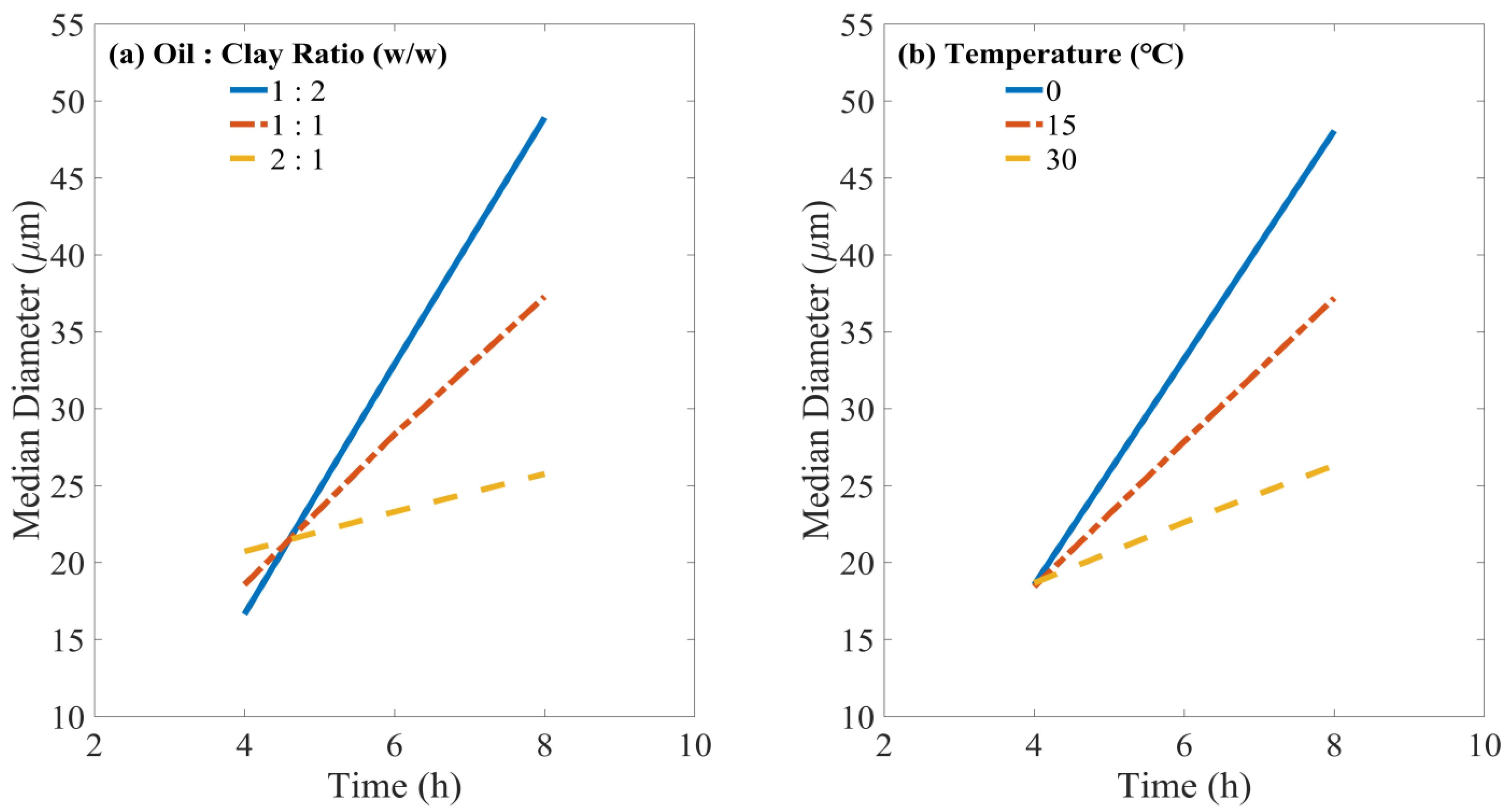
3.1.2. Interaction Effects
This study extended beyond assessing the individual influences of factors by also examining the two-factor interaction effects. Significant interactions, as presented in Table 2, involved combinations of time, oil/clay ratio, and temperature. The influence of these interactions on the D50 of OMA was quantified by Equation (4). For each combination of factor levels, the response value (D50) was computed, with the mean value utilized for analysis. The resulting data are presented in Figure 4. Although the model incorporates interaction terms, it retains linearity concerning its parameters. This linear characteristic stems from the inherent linear properties of statistical modeling within an ANOVA framework, where “linear” suggests a direct relation to the model’s coefficients rather than the predictors. Consequently, a linear relationship between the factor and response is shown in Figure 4.
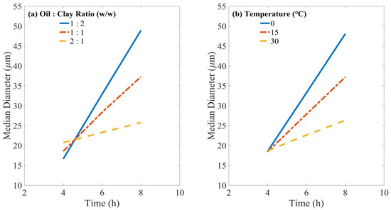
Figure 4.
Illustration of how time interacts with the (a) oil/clay ratio; (b) temperature influence on the median diameter of oil–mineral aggregates.
The statistical analysis presented in Table 2 revealed that the impact of time on D50 was significantly influenced by the oil/clay ratio, as evidenced by the low p-value (0.004) for the interaction between time and the oil/clay ratio. This finding is further supported by the graphical representation in Figure 4a, showing that an increase in the mixing time from 4 h to 8 h did not significantly enhance D50 (~24 µm) at an oil/clay ratio of 2:1. Conversely, a substantial increment in D50 was observed (ranging from ~20 µm to 48 µm) with oil/clay ratios of 1:1 or 1:2. This suggests a significant dependency of the time effect on the oil/clay ratio. Specifically, a higher proportion of clay in the OMA formation system appears to amplify the effect of extended time, resulting in larger OMAs.
Additionally, the impact of time on OMA D50 was significantly influenced by temperature, as indicated by a p-value of 0.02 (Table 2) and demonstrated in Figure 4b. At 0 °C, extending the formation time from 4 to 8 h significantly raised D50 from 20 µm to 47 µm, while at higher temperatures of 15 °C and 30 °C, the increases in D50 were less pronounced. This finding implies that longer formation times at lower temperatures are conducive to forming larger OMAs, whereas the effect of formation time on D50 diminishes with increasing temperature.
Observations from Figure 4a,b reveal that at shorter mixing times (4 h), variations in temperature or oil/clay ratio have a minimal impact on OMA D50. This is possibly due to insufficient duration for the complete development of OMAs during the initial mixing stages. Consequently, the influences of temperature and oil/clay ratio on OMA formation are less noticeable in this early stage. However, as the mixing time extends, the gradual growth in OMA D50 can be attributed to the continuous aggregation of free particles onto the oil droplets or the already formed OMAs [31].
3.2. Machine Learning Prediction
3.2.1. Algorithm Selection
In this study, we investigated the feasibility of employing machine learning algorithms for predicting OMA D50, a topic that has received minimal attention to date. To accomplish this, we utilized three machine learning algorithms, namely RF, GBR, and Adaboost, to estimate OMA D50. The dataset used in this study comprised the data generated in our work and previously published data [16,18,27,28,29,30,31,32], with the D50 size distribution presented in Figure 5. It is evident from Figure 5 that most of the data fell within the 5–80 µm range, while data for OMA D50 in the range of 80–300 µm were limited. The literature experimental conditions and the resulting OMA median diameter are provided in the supplemental Excel file described in the Data Availability Statement section.
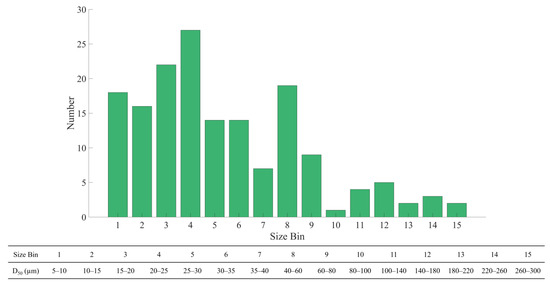
Figure 5.
Size distribution of the dataset from current and literature data [16,18,27,28,29,30,31,32]. The literature experimental conditions and the resulting oil–mineral aggregates’ median diameter is provided in the supplemental Excel file described in the Data Availability Statement section.
The methodological strategy for model selection involved the application of nested CV, enabling the identification of the most effective model. This methodological approach effectively simulates the process of model training and subsequent evaluation on independent datasets, ultimately ensuring a more unbiased estimate of the model’s predictive performance. The R2 scores derived from the nested CV process for each algorithm are presented in Table 3, providing a detailed comparative comparison. It should be emphasized that the nested CV score is derived from the mean of the performance scores yielded from each of the outer “testing” folds. Among the array of evaluated algorithms, the RF exhibited superior performance with an R2 score of 0.930. This performance metric is notably higher than those achieved by the GBR (0.886) and AdaBoost (0.908) algorithms, highlighting the relative effectiveness of the RF approach in this specific setting. Furthermore, the standard deviation of the R2 scores obtained from the nested CV serves as an indicator for model stability. The RF model demonstrated the lowest standard deviation of 0.036, implying a more consistent performance across data folds than the GBR (0.051) and AdaBoost (0.041). In essence, the RF’s performance was less influenced by the specific division of data into training and validation subsets. Consequently, the most efficient model derived from the RF algorithm was retained for subsequent analyses and predictions.
Table 3.
Average score and standard deviation of nested cross-validation (CV) for studied algorithms. The nested CV score is calculated as the average of the performance scores obtained from each of the outer “testing” folds.
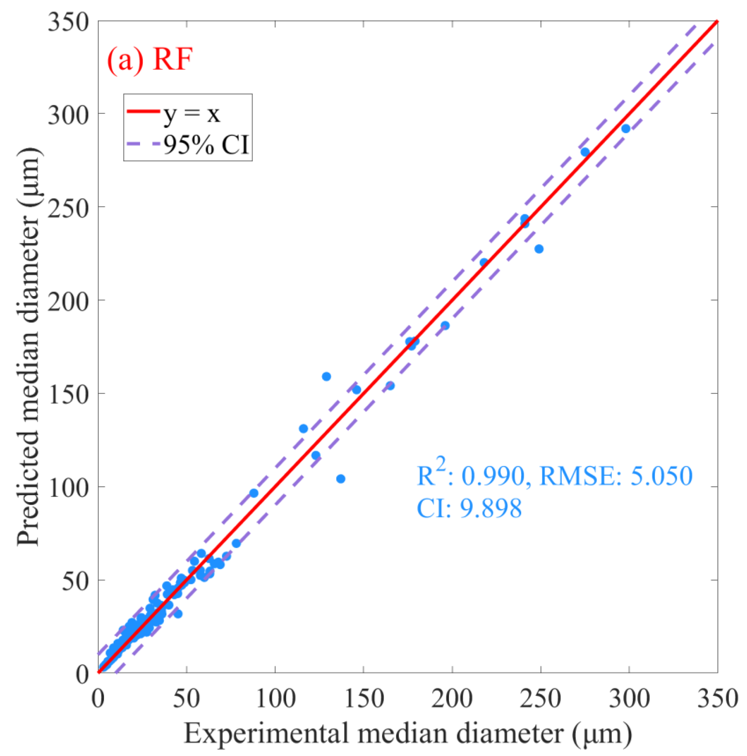
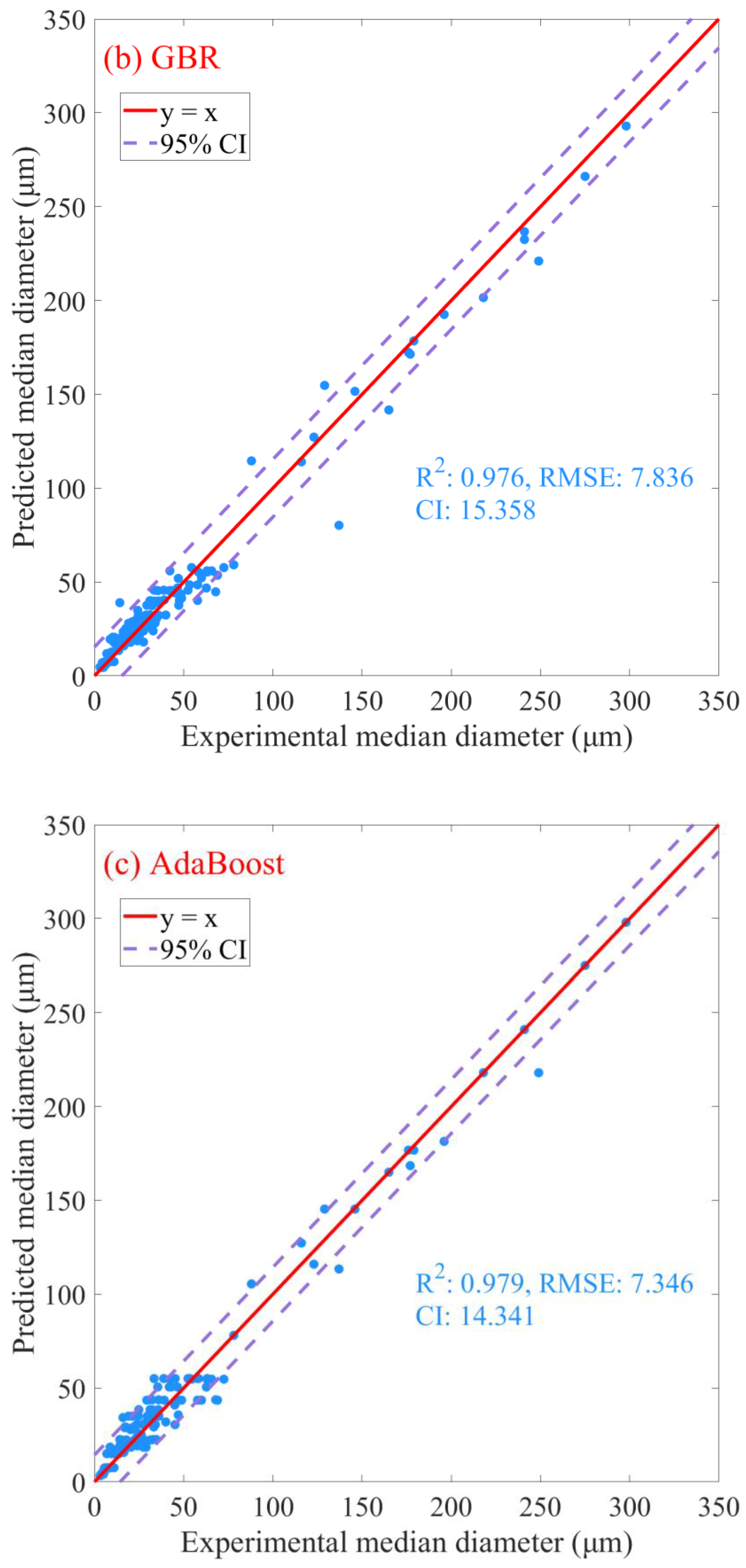
Following the identification of optimal models for each algorithm via nested cross-validation, the predictive capabilities of each model were assessed using the entire original dataset. The predicted results are presented in Figure 6. The RF algorithm presented the highest degree of predictive performance, achieving an R2 score of 0.990 (Figure 6a), signifying that it accounted for 99.0% of the variation in the dependent variables. Additionally, the model’s RMSE was 5.050 (Figure 6a), illustrating high predictive accuracy with a relatively low average squared difference between the observed and predicted values. Lastly, the confidence interval (CI) for the RF model was 9.898 (Figure 6a), emphasizing the model’s precision in predicting outcomes within this range. Comparatively, the GBR and AdaBoost algorithms yield lower R2 values of 0.976 and 0.979 (Figure 6b,c), respectively, implying slightly less variance explanation. Concurrently, both models generated higher RMSE values (GBR: 7.836; AdaBoost: 7.346; Figure 6b,c), implying slightly lower prediction accuracy than the RF model. Regarding CI, both the GBR and AdaBoost models have broader intervals (GBR: 15.359, AdaBoost: 14.341; Figure 6b,c) than the RF model, indicating less precision. Although all three models exhibit high predictive capabilities, the RF model demonstrates a marginally superior performance in terms of accuracy and precision. Therefore, considering the nested CV results and the predictive metrics from the entire dataset, the RF model appears to be the most suitable model for this specific application.
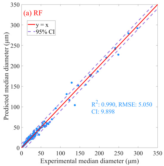
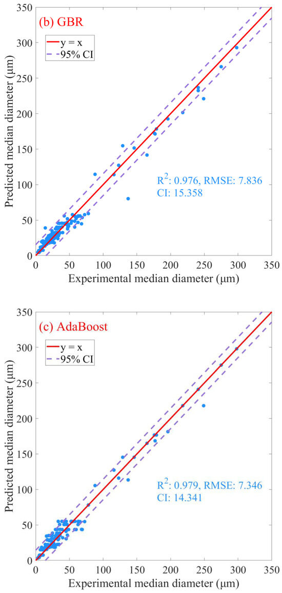
Figure 6.
Prediction plots for oil–mineral aggregates’ median diameter using machine learning algorithms. (a) Random Forest, (b) Gradient Boosting Regression, (c) Adaptive Boosting. R2 denotes coefficient of determination, RMSE denotes root mean square error, and CI denotes the 95% confidence interval.
3.2.2. Sensitivity Analysis of Dataset Partitioning
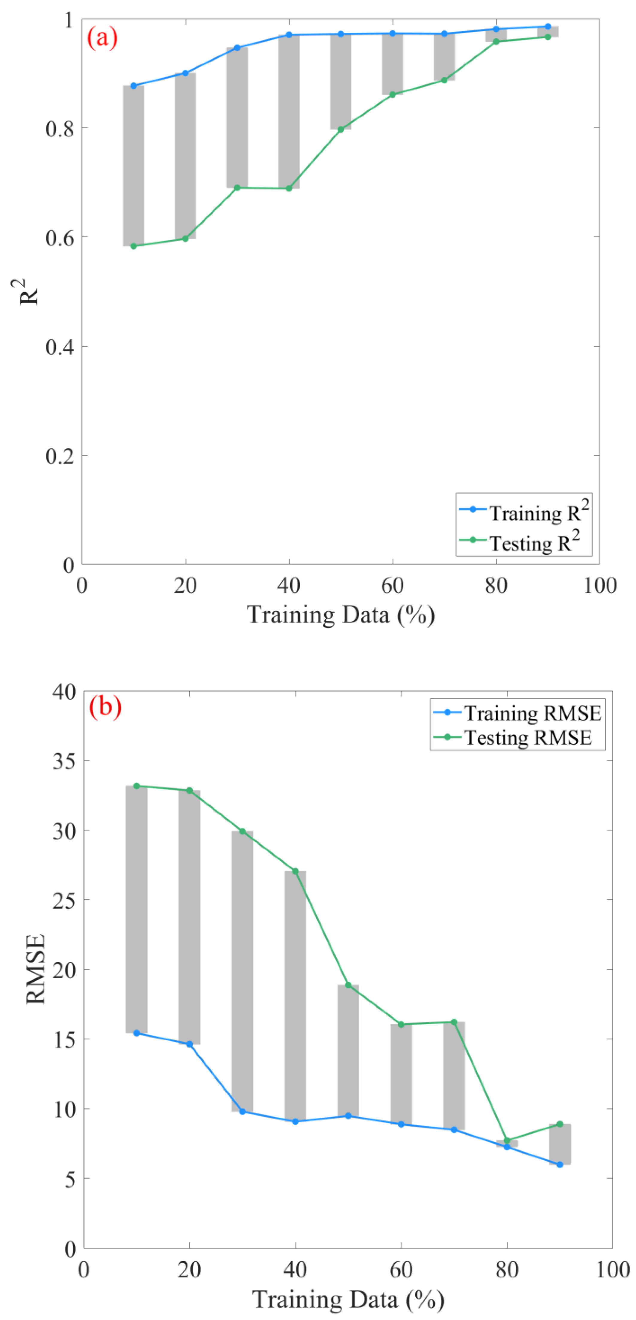
The nested CV strategy produced an RF model with notable predictive capabilities, demonstrated by the highest average R2 values of 0.930 ± 0.036 for unseen data and 0.990 for training data. Nonetheless, it was deemed critical to conduct a sensitivity analysis to assess the stability and reliability of this optimal model, as well as to ascertain the sufficiency and quality of the input dataset by employing various training/testing ratios [43,57].
To facilitate this, a sensitivity analysis was undertaken by systematically adjusting the proportions of the original dataset allocated in the testing set in 10% increments, ranging from 10% to 90%. Conversely, the training set proportion was decremented from an initial 90% to 10% in similar 10% steps. [42,43]. The influence of the partitioning strategy was quantified using R2 and RMSE. The corresponding outcomes are graphically represented in Figure 7a,b. As the proportion allocated to the training dataset increases, a corresponding enhancement occurs in the model’s performance for the training and testing datasets. Specifically, the R2 for the training set increases from 0.878 to 0.986 as the training size increases from 10% to 90%. This increment suggests an enhanced ability of the model to account for the variance in the training data with an increasing data volume. In terms of the testing set performance, there is a substantial improvement in the R2 values, transitioning from 0.583 to 0.967. This suggests an improved generalization capacity of the model. Moreover, it is particularly noteworthy that the performance on the testing set undergoes a more pronounced enhancement when the training set is increased beyond 50% of the total dataset. This emphasizes the significance of a sufficiently sized training dataset to ensure not only a good fit to the training data but also effective generalizability to unseen data. The observations underscore the necessity of partitioning the data, especially in contexts where model predictions are crucial. Concurrently, the training and testing RMSE witnesses a general decline, as shown in Figure 7b, further corroborating the superior fit of the model with enlarged training data. This phenomenon is consistent with previous investigations that an enlarged training set and, consequently, a diminished testing set can result in better model performance [58,59,60]. Additionally, a notable decrease in the testing RMSE to 7.72 occurs when the training size is 80%, representing the minimum across all evaluated sizes. However, increasing the training size to 90% results in a slight increase in RMSE, even though the R2 remains high. This suggests an 80% training size might offer a good trade-off between training and testing performance.
Figure 7.
Evaluation of the dataset partitioning strategy across varied dataset configurations. The robustness of the partitioning strategy is quantitatively illustrated via the (a) coefficient of determination (R2) and (b) root mean square error (RMSE).
The difference between training and testing R2 and RMSE is represented as gray bars in Figure 7a,b. A notable decline in the R2 difference, from 0.30 to 0.02, is observed as the proportion of data allocated for training increases from 10% to 90%. Typically, a narrowing between the training and testing performance metrics suggests a reduction in overfitting and an enhancement in the model’s ability to generalize [61]. In this study, it is evident that as the model is trained on a larger dataset, its ability to make accurate predictions for unseen data (testing set) increases, corroborating its robust stability and superior generalization attributes.
3.2.3. Feature Importance
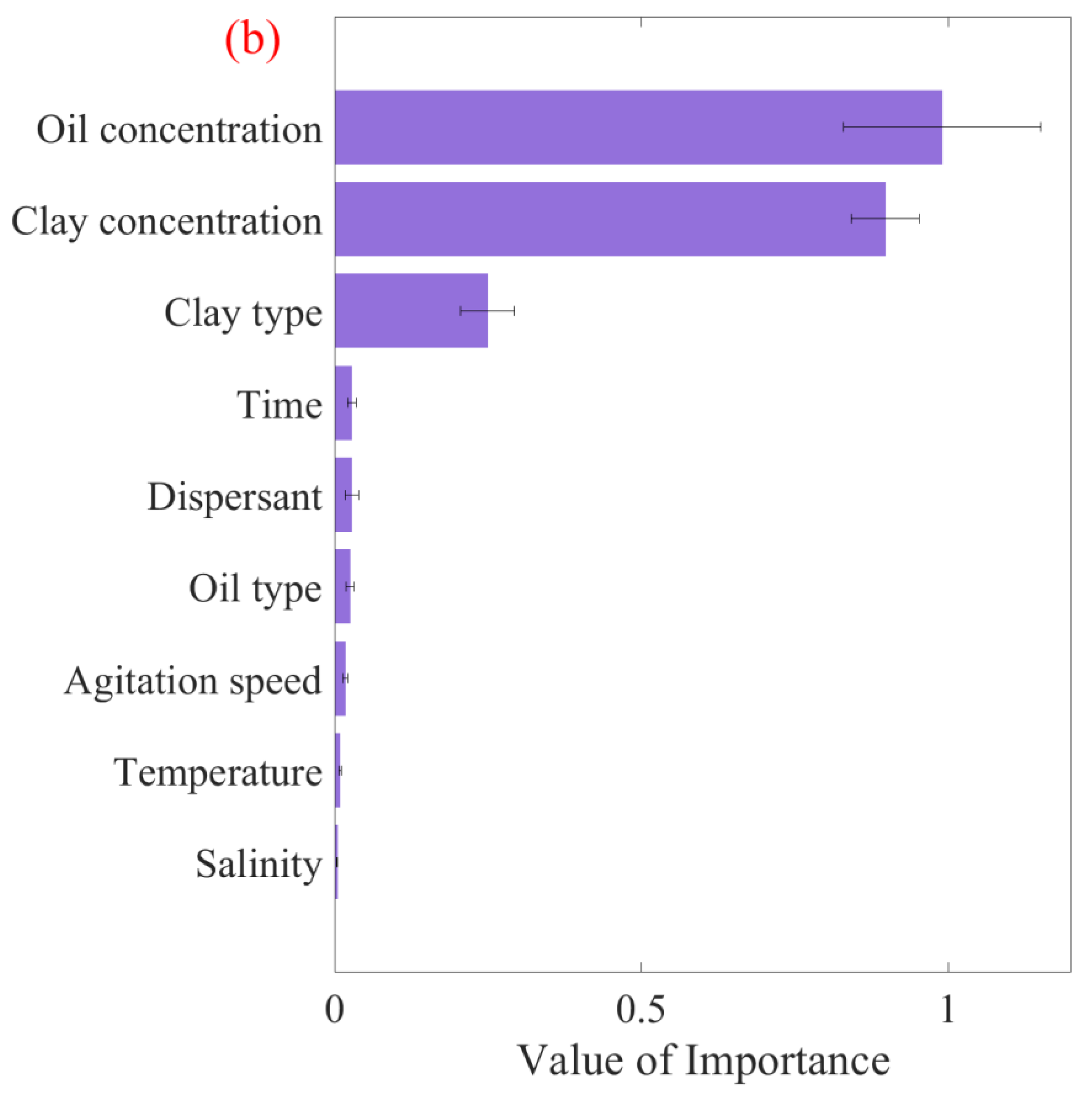
Utilizing the current study and relevant literature, various factors were applied to estimate the D50 of OMAs, including shaking rate, time, temperature, salinity, clay and oil concentrations, clay and oil types (density), and the presence or absence of dispersants. As clarified in Section 3.2.1 and Section 3.2.2, the RF algorithm was identified as the most appropriate method for predicting OMA D50. Through its implementation, the significance of each factor was quantified using conventional and permutation feature importance analyses, as shown in Figure 8. The conventional feature importance results (Figure 8a) indicate that oil concentration, clay concentration, and clay type had the greatest influence on D50, contributing to more than 90% of the outcome. This was consistent with the permutation feature results (Figure 8b), showing that the model’s performance decreased significantly when the oil concentration, clay concentration, and clay type were changed. Consequently, future studies on OMA formation should prioritize these three factors.
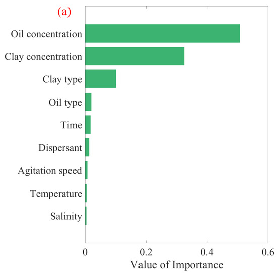
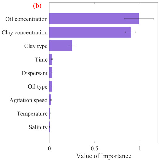
Figure 8.
Factor importance plot derived from the RF algorithm for oil–mineral aggregates’ median diameter using (a) conventional feature importance and (b) permutation feature importance.
The conventional and permutation feature importance analysis methods agree on the most and least important variables for OMA median size, yet they diverge in ranking the intermediate variables. This divergence arises from their inherent methodological differences. The conventional method focuses on model-centric criteria and is well-suited for analyzing how the model processes different data features. This approach is useful for model optimization and understanding its algorithmic behavior. Conversely, the permutation method adopts an empirical approach and is more effective in assessing the real-world impact of feature variations on OMA size. This provides valuable insights for practical application.
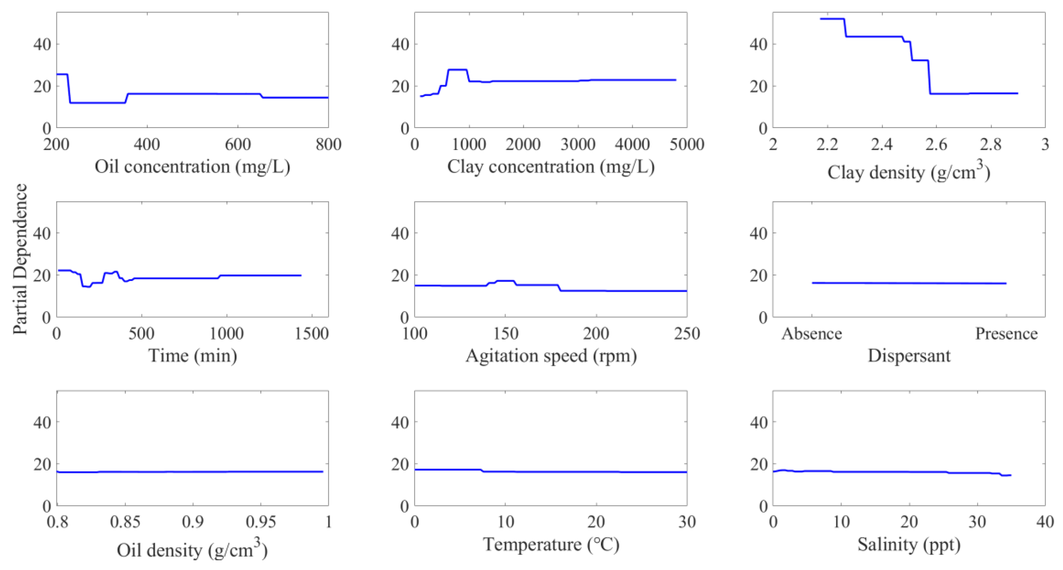
Furthermore, the influence of individual factors on OMA D50 prediction was investigated using PDPs, as shown in Figure 9. These plots illustrate the partial dependence of a single predictor variable on the predicted response of a machine learning model while controlling for the values of other predictor variables. A noteworthy observation was the decline in predicted OMA D50 from approximately 25 µm to 11 µm with an increase in oil concentration from 200 mg/L to ~250 mg/L. Beyond this, a further rise in oil concentration did not markedly influence the OMA median size. Given the limited studies on this particular impact of oil concentration, additional investigations are required.
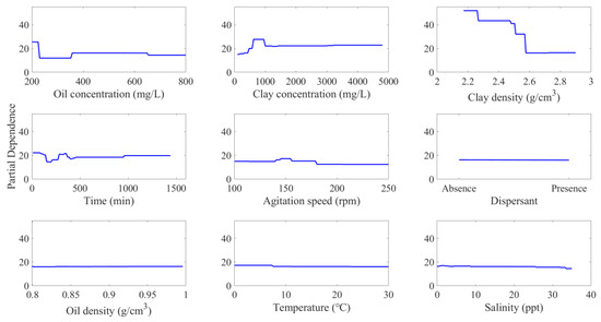
Figure 9.
Partial dependence plots (PDPs) for studied factors on oil–mineral aggregates’ median diameter prediction.
Regarding clay concentration, an uptrend was observed in OMA median size, peaking at ~800 mg/L. Further increments to 1200 mg/L showed a reduction in the median size, beyond which OMA D50 largely remained invariant. This observation parallels findings from Guyomarch et al. (2002), who claimed a Gaussian distribution for average OMA size, with the peak at a clay concentration of 800 mg/L [34].
For clay type (density), as illustrated in Figure 9, there is a noticeable stratified reduction in OMA D50 from approximately 50 µm to 15 µm with increasing clay density. This observation was consistent with prior research where OMAs formed by silica (density = 2.46 g/cm3) presented a larger median size compared to that by kaolinite (density = 2.63 g/cm3) [49]. Nonetheless, most prior studies have focused on properties like clay hydrophobicity and cation exchange capacity rather than clay density and its implications on the OMA size distribution [37,49,53].
Both agitation time and speed exhibited slight influences on OMA D50, particularly at their lower values. As shown in Figure 9, OMA D50 remained relatively consistent initially, followed by a minor decrease between 1.5 and 3 h. Subsequent to this, there was a gradual increase in OMA D50, peaking at 6 h, beyond which it stabilized with prolonged agitation. This behavior is similar to earlier observations where OMAs form rapidly at the initial 3 h, followed by their breaking apart. With prolonged agitation, the reformation of OMAs was observed, potentially due to the increased presence of oil droplets on the water surface [28]. In relation to agitation speed, a reasonable increase in OMA median size was noted until reaching peaking at approximately 150 rpm. Beyond this point, OMA median size exhibited a reduction with increased agitation speed. This can be explained by acknowledging that an optimal agitation speed promotes OMA formation [31], whereas an overly aggressive agitation speed might lead to OMA breakage [22].
As illustrated in Figure 9, the effects of several parameters, namely the presence of dispersants, oil type (density), temperature, and salinity, on the median size of OMAs were evident. The role of dispersants in affecting OMA size has been a point of contention in existing literature [16,17,18,19,20,62]. In this analysis, OMA D50 data were collected from multiple studies, each employing varied dispersant types and differing dispersant-to-oil ratios (DOR). This variability could be a primary reason for the RF model’s inability to accurately reflect the dispersant’s influence on the median OMA size. Similarly, salinity’s effect on OMA size has been inconsistent across different studies [22,29,63,64,65], potentially impacting the PDPs for salinity concerning OMA median diameter. The influence of oil type on OMA’s median size appeared negligible, supporting prior studies that suggest that the oil type does not significantly impact OMA size [18]. It was further observed that OMA sizes under colder conditions were marginally larger compared to those at higher temperatures. This observation resonates with previous findings [30] and can be attributed to the decrease in oil viscosity with a rise in temperature, enhancing the dispersion of oil into finer droplets. Consequently, the D50 of OMA demonstrates a reduction with temperature increase.
The feature importance derived from the machine learning algorithm and the significant factors identified through statistical analysis underscores the importance of oil and clay concentrations (correlating closely with the oil/clay ratio) and clay type. However, there are subtle differences in the results concerning other factors when comparing the two methodologies. This variation may be attributed to differences in data sources and the investigation range.
3.3. Machine Learning-Based Prediction Software
As Section 3.2.1 and Section 3.2.2 demonstrated, the RF algorithm exhibits satisfactory predictive capability for OMA D50, registering R2 values of 0.93 for unseen data and 0.99 for training data. Based on these observations, a software application incorporating the RF algorithm was developed to optimize the predictive workflow. A visual representation of the software’s user interface is illustrated in Figure 10. This tool expedites the estimation of OMA D50 by permitting users to input relevant formation process parameters. Available as an executable (.exe) file in the Data Availability Statement section. This open-source software can be easily downloaded on a user’s computer for convenient use.
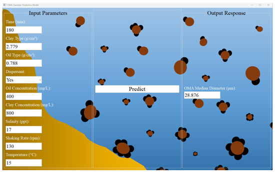
Figure 10.
Screenshot of the software application for oil–mineral aggregates’ median diameter prediction.
4. Conclusions
This research utilized a screening design to methodically investigate the formation of oil–mineral aggregates (OMAs) and identify the most influential factors. Seven process variables were analyzed, including temperature, time, salinity, clay type, agitation speed, oil/clay weight ratio, and the presence or absence of dispersants. The findings indicated that time exerted the most significant influence on the median diameter of OMAs, with temperature and oil/clay ratio also important factors. Notably, the effect of time was heavily influenced by the specific temperature and oil/clay ratio. Extending the mixing time to 8 h, particularly at a low temperature of 0 °C and an oil/clay ratio of 1:2, resulted in a significantly larger OMA D50 (approximately 50 µm).
Furthermore, this study evaluated the possibility of employing machine learning algorithms for OMA median diameter prediction for the first time. Three tree-based machine learning algorithms, including Random Forest (RF), Gradient Boosting Regression (GBR), and Adaboost, were assessed. The nested CV method was applied to identify the most effective model. RF demonstrated the most satisfactory performance predicting D50, with high R2 values (0.93 for unseen data and 0.99 for training data) and low RMSE values. The stability and generalizability of this optimal RF model were investigated using various test/train splitting. The results indicated that as the model is trained on a larger dataset, the RF model’s talent in making accurate predictions on previously unseen data (testing set) increases, corroborating its robust stability and superior generalizability.
The RF algorithm was employed to quantify the significance of each process factor. The outcomes from conventional and permutation feature importance analyses concurred, highlighting the concentration of oil and clay and clay type as the most important factors in predicting the median size of OMAs in this investigation. Furthermore, partial dependence plots (PDPs) were utilized to assess the influence of individual variables on OMA median size prediction. The observed trends for several factors, such as clay concentration and type and agitation time and speed, were consistent with existing literature. However, future research is needed to further examine the influence of these factors on OMA size prediction.
This research also led to the development of an open-source software application incorporating the RF algorithm. This tool, designed for user-friendly installation on personal computers, facilitates rapid predictions of OMA D50 based on input formation process variables. Despite its utility, further research is needed to expand the dataset and refine the model for enhanced predictive accuracy.
Overall, this multi-disciplinary research successfully identified key factors and their interactions influencing the formation of OMAs. Furthermore, it innovatively incorporated machine learning algorithms for the prediction of OMA median diameter. The findings and the practical tools developed in this study demonstrate significant potential for future, more detailed investigations of OMAs, particularly regarding size distribution. These advancements are important in enhancing the accuracy of tracking the fate and trajectory of oil spills, contributing significantly to the field of environmental monitoring and remediation.
Supplementary Materials
The following supporting information can be downloaded at: https://www.mdpi.com/article/10.3390/jmse12010144/s1, Table S1. The experiment’s setting is based on Screening Design; Figure S1. The temperature controllable shaker; Figure S2. The inverted microscopy.
Author Contributions
Conceptualization, X.Z. and Y.W.; methodology, X.Z. and J.Y.; software, X.Z.; validation, Y.W., H.N. and L.L.; formal analysis, X.Z. and J.Y.; investigation, X.Z. and H.N.; resources, H.N. and L.L.; data curation, X.Z. and J.Y.; writing—original draft preparation, X.Z.; writing—review and editing, X.Z., Y.W. and H.N.; visualization, X.Z.; supervision, H.N.; project administration, H.N.; funding acquisition, H.N. and L.L. All authors have read and agreed to the published version of the manuscript.
Funding
This research was funded by the Marine Environment Observation Prediction and Response Network (MEOPAR, 2-02-03-0373) and Multi-Partner Research Initiative (MPRI 6.02).
Institutional Review Board Statement
Not applicable.
Informed Consent Statement
Not applicable.
Data Availability Statement
The present and literature experimental conditions and the resulting oil–mineral aggregates’ median diameter is openly available in Google Drive at [https://docs.google.com/spreadsheets/d/19eGvo1Z_hcgkBNnKXURapWjj_fW0aUZG/edit?usp=sharing&ouid=117372061656087239227&rtpof=true&sd=true]. An open-source software application that incorporated the RF algorithm is openly available in Google Drive at [https://drive.google.com/file/d/1uzMRLwD-Q7oGiIW4yOGyhVM0AhRGwQ9z/view?usp=sharing].
Acknowledgments
The authors are grateful for the financial support from the Marine Environment Observation Prediction and Response Network and Multi-Partner Research Initiative.
Conflicts of Interest
The authors declare no conflict of interest.
References
- ITOPF. Oil Tanker Spill Statistics 2021; International Tanker Owners Pollution Federation (ITOPF): London, UK, 2022; Available online: https://www.itopf.org/fileadmin/uploads/itopf/data/Documents/Company_Lit/Oil_Spill_Stats_2021.pdf (accessed on 12 January 2023).
- Kingston, P.F. Long-Term Environmental Impact of Oil Spills. Spill Sci. Technol. Bull. 2002, 7, 53–61. [Google Scholar] [CrossRef]
- Bragg, J.R.; Owens, E.H. Shoreline Cleansing by Interactions Between Oil and Fine Mineral Particles. Int. Oil Spill Conf. Proc. 1995, 1995, 219–227. [Google Scholar] [CrossRef]
- Lee, K.; Stoffyn-Egli, P.; Wood, P.A.; Lunel, T. Formation and Structure of Oil-Mineral Fines Aggregates in Coastal Environments; Environment Canada: Ottawa, ON, Canada, 1998; pp. 911–921.
- Owens, E.H. The Interaction of Fine Particles with Stranded Oil. Pure Appl. Chem. 1999, 71, 83–93. [Google Scholar] [CrossRef]
- Payne, J.R.; Kirstein, B.E.; Clayton, J.R.; Clary, C.; Redding, R. Integration of Suspended-Particulate Matter and Oil-Transportation Study. Final Report, September 1984–September 1987; Science Applications International Corp.: San Diego, CA, USA, 1987. [Google Scholar]
- Poirier, O.A.; Thiel, G.A. Deposition of Free Oil by Sediments Settling in Sea Water. AAPG Bull. 1941, 25, 2170–2180. [Google Scholar]
- Sterling, M.C.; Bonner, J.S.; Ernest, A.N.S.; Page, C.A.; Autenrieth, R.L. Application of Fractal Flocculation and Vertical Transport Model to Aquatic Sol–Sediment Systems. Water Res. 2005, 39, 1818–1830. [Google Scholar] [CrossRef]
- Spaulding, M.L. State of the Art Review and Future Directions in Oil Spill Modeling. Mar. Pollut. Bull. 2017, 115, 7–19. [Google Scholar] [CrossRef] [PubMed]
- Bragg, J.R.; Yang, S.H.; Roffall, J.C. Experimental Studies of Natural Cleansing of Oil Residue from Rocks in Prince William Sound by Wave/Tidal Action: Unpublished Report; Exxon Production Research Co.: Richardson, TX, USA, 1990; Volume 2189. [Google Scholar]
- Jahns, H.O.; Bragg, J.R.; Dash, L.C.; Owens, E.H. Natural Cleaning of Shorelines Following the Exxon Valdez Spill. Int. Oil Spill Conf. Proc. 1991, 1991, 167–176. [Google Scholar] [CrossRef]
- Bragg, J.R.; Yang, S.H. Clay Oil Flocculation and Its Role in Natural Cleansing in Prince William Sound Following the Exxon Valdez Oil Spill; American Society for Testing and Materials: West Conshohocken, PA, USA, 1995; Volume 28, pp. 178–214. [Google Scholar]
- Lee, K. Oil–Particle Interactions in Aquatic Environments: Influence on the Transport, Fate, Effect and Remediation of Oil Spills. Spill Sci. Technol. Bull. 2002, 8, 3–8. [Google Scholar] [CrossRef]
- Gong, Y.; Zhao, X.; Cai, Z.; O’Reilly, S.E.; Hao, X.; Zhao, D. A Review of Oil, Dispersed Oil and Sediment Interactions in the Aquatic Environment: Influence on the Fate, Transport and Remediation of Oil Spills. Mar. Pollut. Bull. 2014, 79, 16–33. [Google Scholar] [CrossRef]
- Zhong, X.; Niu, H.; Li, P.; Wu, Y.; Liu, L. An Overview of Oil-Mineral-Aggregate Formation, Settling, and Transport Processes in Marine Oil Spill Models. J. Mar. Sci. Eng. 2022, 10, 610. [Google Scholar] [CrossRef]
- Khelifa, A.; Stoffyn-Egli, P.; Hill, P.S.; Lee, K. Characteristics of Oil Droplets Stabilized by Mineral Particles: The Effect of Salinity. Int. Oil Spill Conf. Proc. 2003, 2003, 963–970. [Google Scholar] [CrossRef]
- Le-Floch, S.; Guyomarch, J.; Merlin, F.-X.; Stoffyn-Egli, P.; Dixon, J.; Lee, K. The Influence of Salinity on Oil–Mineral Aggregate Formation. Spill Sci. Technol. Bull. 2002, 8, 65–71. [Google Scholar] [CrossRef]
- Khelifa, A.; Stoffyn-Egli, P.; Hill, P.S.; Lee, K. Effects of Salinity and Clay Type on Oil–Mineral Aggregation. Mar. Environ. Res. 2005, 59, 235–254. [Google Scholar] [CrossRef]
- Kerebel, D. Study of the Influence of Salinity on the Flocculation Oil-Clay; Final Rep. Fr. 20p Annex; Centre de Documentation de Recherche et D’Expérimentations sur les Pollutions Accidentelles des Eaux (Cèdre): Brest, France, 1997. [Google Scholar]
- Guyomarch, J.; Merlin, F.-X.; Bernanose, P. Oil Interaction with Mineral Fines and Chemical Dispersion: Behaviour of the Dispersed Oil in Coastal or Estuarine Conditions. In Proceedings of the AMOP—Arctic and Marine Oil Spill Technical Seminar, Calgary, AB, Canada, 2–4 June 1999; Ministry of Supply and Services: Toronto, ON, Canada, 1999; Volume 1, pp. 137–150. [Google Scholar]
- Qi, Z.; Wang, Z.; Yu, Y.; Yu, X.; Sun, R.; Wang, K.; Xiong, D. Formation of Oil-Particle Aggregates in the Presence of Marine Algae. Environ. Sci. Process. Impacts 2023, 25, 1438–1448. [Google Scholar] [CrossRef] [PubMed]
- Zhang, H.; Khatibi, M.; Zheng, Y.; Lee, K.; Li, Z.; Mullin, J.V. Investigation of OMA Formation and the Effect of Minerals. Mar. Pollut. Bull. 2010, 60, 1433–1441. [Google Scholar] [CrossRef]
- Blainey, P.; Krzywinski, M.; Altman, N. Replication. Nat. Methods 2014, 11, 879–880. [Google Scholar] [CrossRef] [PubMed]
- Cao, Y.; Kang, Q.; Zhang, B.; Zhu, Z.; Dong, G.; Cai, Q.; Lee, K.; Chen, B. Machine Learning-Aided Causal Inference for Unraveling Chemical Dispersant and Salinity Effects on Crude Oil Biodegradation. Bioresour. Technol. 2022, 345, 126468. [Google Scholar] [CrossRef]
- Loh, W.S.; Chin, R.J.; Ling, L.; Lai, S.H.; Soo, E.Z.X. Application of Machine Learning Model for the Prediction of Settling Velocity of Fine Sediments. Mathematics 2021, 9, 3141. [Google Scholar] [CrossRef]
- Yu, J.; Zhong, X.; Huang, Z.; Lin, X.; Weng, H.; Ye, D.; He, Q.S.; Yang, J. Mining the Synergistic Effect in Hydrothermal Co-Liquefaction of Real Feedstocks through Machine Learning Approaches. Fuel 2023, 334, 126715. [Google Scholar] [CrossRef]
- Jézéquel, R.; Receveur, J.; Nedwed, T.; Le Floch, S. Evaluation of the Ability of Calcite, Bentonite and Barite to Enhance Oil Dispersion under Arctic Conditions. Mar. Pollut. Bull. 2018, 127, 626–636. [Google Scholar] [CrossRef]
- Ji, W.; Boufadel, M.; Zhao, L.; Robinson, B.; King, T.; An, C.; Zhang, B.H.; Lee, K. Formation of Oil-Particle Aggregates: Impacts of Mixing Energy and Duration. Sci. Total Environ. 2021, 795, 148781. [Google Scholar] [CrossRef]
- Khelifa, A.; Fingas, M.; Brown, C. Effects of Dispersants on Oil-SPM Aggregation and Fate in US Coastal Waters; Final Report Grant Number NA04NOS4190063; University of New Hampshire: Durham, NH, USA, 2008. [Google Scholar]
- Khelifa, A.; Stoffyn-Egli, P.; Hill, P.S.; Lee, K. Characteristics of Oil Droplets Stabilized by Mineral Particles: Effects of Oil Type and Temperature. Spill Sci. Technol. Bull. 2002, 8, 19–30. [Google Scholar] [CrossRef]
- Sun, J.; Khelifa, A.; Zhao, C.; Zhao, D.; Wang, Z. Laboratory Investigation of Oil–Suspended Particulate Matter Aggregation under Different Mixing Conditions. Sci. Total Environ. 2014, 473–474, 742–749. [Google Scholar] [CrossRef]
- Wang, W.; Zheng, Y.; Lee, K. Chemical Dispersion of Oil with Mineral Fines in a Low Temperature Environment. Mar. Pollut. Bull. 2013, 72, 205–212. [Google Scholar] [CrossRef] [PubMed]
- Murray, H.H. Traditional and New Applications for Kaolin, Smectite, and Palygorskite: A General Overview. Appl. Clay Sci. 2000, 17, 207–221. [Google Scholar] [CrossRef]
- Guyomarch, J.; Le Floch, S.; Merlin, F.-X. Effect of Suspended Mineral Load, Water Salinity and Oil Type on the Size of Oil–Mineral Aggregates in the Presence of Chemical Dispersant. Spill Sci. Technol. Bull. 2002, 8, 95–100. [Google Scholar] [CrossRef]
- SeaTemperature.org. World Water Temperature &|Sea Temperatures. Available online: https://www.seatemperature.org/ (accessed on 20 April 2023).
- Sun, J.; Khelifa, A.; Zheng, X.; Wang, Z.; So, L.L.; Wong, S.; Yang, C.; Fieldhouse, B. A Laboratory Study on the Kinetics of the Formation of Oil-Suspended Particulate Matter Aggregates Using the NIST-1941b Sediment. Mar. Pollut. Bull. 2010, 60, 1701–1707. [Google Scholar] [CrossRef]
- Yu, Y.; Qi, Z.; Xiong, D.; Li, W.; Yu, X.; Sun, R. Experimental Investigations on the Vertical Distribution and Properties of Oil-Mineral Aggregates (OMAs) Formed by Different Clay Minerals. J. Environ. Manag. 2022, 311, 114844. [Google Scholar] [CrossRef]
- Sterling, M.C.; Bonner, J.S.; Ernest, A.N.S.; Page, C.A.; Autenrieth, R.L. Characterizing Aquatic Sediment–Oil Aggregates Using in Situ Instruments. Mar. Pollut. Bull. 2004, 48, 533–542. [Google Scholar] [CrossRef]
- Zhang, W.; Yu, X.; Zhang, J.; Wang, Y. Study of Oil-Particle-Aggregation by Digital Inline Holograph. Geosci. J. 2019, 23, 461–469. [Google Scholar] [CrossRef]
- Pedregosa, F.; Varoquaux, G.; Gramfort, A.; Michel, V.; Thirion, B.; Grisel, O.; Blondel, M.; Prettenhofer, P.; Weiss, R.; Dubourg, V.; et al. Scikit-Learn: Machine Learning in Python. J. Mach. Learn. Res. 2011, 12, 2825–2830. [Google Scholar]
- Staartjes, V.E.; Kernbach, J.M. Foundations of Machine Learning-Based Clinical Prediction Modeling: Part III—Model Evaluation and Other Points of Significance. In Machine Learning in Clinical Neuroscience; Staartjes, V.E., Regli, L., Serra, C., Eds.; Springer International Publishing: Cham, Switzerland, 2022; pp. 23–31. [Google Scholar]
- Ahmad, H. Machine Learning Applications in Oceanography. Aquat. Res. 2019, 2, 161–169. [Google Scholar] [CrossRef]
- Nguyen, Q.H.; Ly, H.-B.; Ho, L.S.; Al-Ansari, N.; Le, H.V.; Tran, V.Q.; Prakash, I.; Pham, B.T. Influence of Data Splitting on Performance of Machine Learning Models in Prediction of Shear Strength of Soil. Math. Probl. Eng. 2021, 2021, e4832864. [Google Scholar] [CrossRef]
- Delvigne, G.A.L.; Sweeney, C.E. Natural Dispersion of Oil. Oil Chem. Pollut. 1988, 4, 281–310. [Google Scholar] [CrossRef]
- Zhao, L.; Torlapati, J.; Boufadel, M.C.; King, T.; Robinson, B.; Lee, K. VDROP: A Comprehensive Model for Droplet Formation of Oils and Gases in Liquids—Incorporation of the Interfacial Tension and Droplet Viscosity. Chem. Eng. J. 2014, 253, 93–106. [Google Scholar] [CrossRef]
- Sathyagal, A.N.; Ramkrishna, D.; Narsimhan, G. Droplet Breakage in Stirred Dispersions. Breakage Functions from Experimental Drop-Size Distributions. Chem. Eng. Sci. 1996, 51, 1377–1391. [Google Scholar] [CrossRef]
- Al-Besharah, J.M.; Akashah, S.A.; Mumford, C.J. The Effect of Temperature and Pressure on the Viscosities of Crude Oils and Their Mixtures. Ind. Eng. Chem. Res. 1989, 28, 213–221. [Google Scholar] [CrossRef]
- Hassan, M.E.; Nielsen, R.F.; Calhoun, J.C. Effect of Pressure and Temperature on Oil-Water Interfacial Tensions for a Series of Hydrocarbons. J. Pet. Technol. 1953, 5, 299–306. [Google Scholar] [CrossRef]
- Ji, W.; Boufadel, M.; Zhao, L.; Robinson, B.; King, T.; Lee, K. Formation of Oil-Particle Aggregates: Particle Penetration and Impact of Particle Properties and Particle-to-Oil Concentration Ratios. Sci. Total Environ. 2021, 760, 144047. [Google Scholar] [CrossRef]
- Zhao, L.; Boufadel, M.C.; Katz, J.; Haspel, G.; Lee, K.; King, T.; Robinson, B. A New Mechanism of Sediment Attachment to Oil in Turbulent Flows: Projectile Particles. Environ. Sci. Technol. 2017, 51, 11020–11028. [Google Scholar] [CrossRef]
- Wang, W.; Zheng, Y.; Li, Z.; Lee, K. PIV Investigation of Oil–Mineral Interaction for an Oil Spill Application. Chem. Eng. J. 2011, 170, 241–249. [Google Scholar] [CrossRef]
- Khabbazi Basmenj, A.; Mirjavan, A.; Ghafoori, M.; Cheshomi, A. Assessment of the Adhesion Potential of Kaolinite and Montmorillonite Using a Pull-out Test Device. Bull. Eng. Geol. Environ. 2017, 76, 1507–1519. [Google Scholar] [CrossRef]
- Stoffyn-Egli, P.; Lee, K. Formation and Characterization of Oil–Mineral Aggregates. Spill Sci. Technol. Bull. 2002, 8, 31–44. [Google Scholar] [CrossRef]
- Kooistra, A.; Verhoef, P.N.W.; Broere, W.; Ngan-Tillard, D.J.M.; van Tol, A.F. Appraisal of Stickiness of Natural Clays from Laboratory Tests. Publ. Appl. Earth Sci. Sect. Eng. Geol. 1998. Available online: https://repository.tudelft.nl/islandora/object/uuid%3A32392fb8-92e7-469d-b78c-b65635f59272 (accessed on 8 January 2024).
- Brandenburg, U.; Lagaly, G. Rheological Properties of Sodium Montmorillonite Dispersions. Appl. Clay Sci. 1988, 3, 263–279. [Google Scholar] [CrossRef]
- Nascimento, G.M.D. Basics of Clay Minerals and Their Characteristic Properties. In Clay and Clay Minerals; BoD—Books on Demand: Norderstedt, Germany, 2021; ISBN 978-1-83969-563-6. [Google Scholar]
- Mohanty, S.P.; Hughes, D.P.; Salathé, M. Using Deep Learning for Image-Based Plant Disease Detection. Front. Plant Sci. 2016, 7, 1419. [Google Scholar] [CrossRef]
- Anifowose, F.; Khoukhi, A.; Abdulraheem, A. Investigating the Effect of Training–Testing Data Stratification on the Performance of Soft Computing Techniques: An Experimental Study. J. Exp. Theor. Artif. Intell. 2017, 29, 517–535. [Google Scholar] [CrossRef]
- Cawley, G.C.; Talbot, N.L.C. On Over-FItting in Model Selection and Subsequent Selection Bias in Performance Evaluation. J. Mach. Learn. Res. 2010, 11, 2079–2107. [Google Scholar]
- Ramezan, C.A.; Warner, T.A.; Maxwell, A.E.; Price, B.S. Effects of Training Set Size on Supervised Machine-Learning Land-Cover Classification of Large-Area High-Resolution Remotely Sensed Data. Remote Sens. 2021, 13, 368. [Google Scholar] [CrossRef]
- Kernbach, J.M.; Staartjes, V.E. Foundations of Machine Learning-Based Clinical Prediction Modeling: Part II—Generalizationng and Overfitting. In Machine Learning in Clinical Neuroscience; Staartjes, V.E., Regli, L., Serra, C., Eds.; Springer International Publishing: Cham, Switzerland, 2022; pp. 15–21. [Google Scholar]
- Payne, J.R. Oil-Ice-Sediment Interactions during Freezeup and Breakup; Final Report, Outer Continental Shelf Environmental Assessment Program; Applied Environmental Sciences Department, Science Applications International Corporation: San Diego, CA, USA, 1989; Volume 64. [Google Scholar]
- Fu, J.; Gong, Y.; Zhao, X.; O’Reilly, S.E.; Zhao, D. Effects of Oil and Dispersant on Formation of Marine Oil Snow and Transport of Oil Hydrocarbons. Environ. Sci. Technol. 2014, 48, 14392–14399. [Google Scholar] [CrossRef]
- Lee, K.; Li, Z.; King, T.; Kepkay, P.; Boufadel, M.C.; Venosa, A.D. Wave Tank Studies on Formation and Transport of OMA from the Chemically Dispersed Oil. In Oil Spill Response: A Global Perspective; Davidson, W.F., Lee, K., Cogswell, A., Eds.; Springer: Dordrecht, The Netherlands, 2008; pp. 159–177. [Google Scholar]
- Page, C.A.; Bonner, J.S.; Sumner, P.L.; McDonald, T.J.; Autenrieth, R.L.; Fuller, C.B. Behavior of a Chemically-Dispersed Oil and a Whole Oil on a near-Shore Environment. Water Res. 2000, 34, 2507–2516. [Google Scholar] [CrossRef]


Disclaimer/Publisher’s Note: The statements, opinions and data contained in all publications are solely those of the individual author(s) and contributor(s) and not of MDPI and/or the editor(s). MDPI and/or the editor(s) disclaim responsibility for any injury to people or property resulting from any ideas, methods, instructions or products referred to in the content. |
© 2024 by the authors. Licensee MDPI, Basel, Switzerland. This article is an open access article distributed under the terms and conditions of the Creative Commons Attribution (CC BY) license (https://creativecommons.org/licenses/by/4.0/).