Abstract
Icebreaking by using underwater explosion bubbles and compressed high-pressure gas bubbles has gradually become an effective icebreaking method. In order to compare the damaging effect of these two methods on the ice body, a fluid–structure coupling model was established based on the arbitrary Lagrangian–Eulerian (ALE) method and a series of calculations were carried out. The morphological changes of underwater explosion bubbles and compressed gas bubbles at the same energy under the free surface; the changes of flow load near the rigid wall; and the damage caused to the ice plate were studied and compared. The damage effect of the ice plate was analyzed by detecting the number of failure elements of the ice plate, and the optimum standoff distance was found. For an ice plate with a radius of 0.19 m and a thickness of 0.15 m, the optimum standoff distance of the compressed gas bubbles with 120 J is 0.03 m, and the optimum standoff distance of the TNT with 120 J is 0.02875 m. The similarities and differences of the two sources of bubbles on ice plate damage were summarized.
1. Introduction
Icebreaking in the Arctic has always been a difficult problem. Traditional icebreaking methods mainly rely on their strength to hit the ice; icebreaking efficiency is low and there is a risk of hull rupture [1,2,3]. Underwater explosives have become a new icebreaking method due to developments in science and technology. In recent years, a high-pressure bubble icebreaking method was developed [4,5,6]. Studies have shown that, among other advantages, the new icebreaking method has directionality [7,8], and is safe and pollution-free [9].
Underwater explosive icebreaking has been widely used to break river ice. Nikolaev [10] proposed using spaced explosions for directional icebreaking to clear channels. At the U.S. Army Cold Regions Research and Engineering Laboratory (CRREL), Mellor [11,12] analyzed the effect of the explosive weight, the submergence depth of the charge and the thickness of the ice sheet to the ice-breaking radius by summarizing the past experimental data. The dimensionless and regression analysis of the data was carried out, and the empirical formula affecting the ice-breaking radius was finally obtained. Wang et al. [13] carried out an offshore test of icebreaking by underwater explosions, and the correlations between different factors of explosive mass, blast distance, ice thickness, and icebreaking radius were calculated with the outfield test and grey system theory. The influence and relationship between the three factors of ice were derived, providing new insights for the optimization of underwater blasting icebreaking parameters.
The development of high-pressure bubble icebreaking methods as an alternative to underwater explosive icebreaking was necessary, due to the unsafe nature of explosive operations and the harmful substances released into the environment.
Due to the complexity of high-pressure icebreaking technology, there are very few studies in the early research literature. Mellor and Kovacs [14] used compressed air and carbon dioxide blasting devices in New Hampshire and Alaska on frozen lakes; it was found that the ice was mainly damaged in terms of bending strength when gas-blasted, and that the diameter of the ice fragments was also larger. In recent years, the concept and connotation of high-pressure gas bubble icebreaking methods have been enriched based on their predecessors. In experiments, electric bubbles and high-pressure air gun bubbles are often used as the bubble source in icebreaking experiments with high-pressure bubbles. Zhang et al. [15,16,17,18] provided a strong research basis and theoretical support for experimental research on the coupling of high-pressure bubbles and structures. Cui et al., Yuan et al., and Ni et al. [4,8,19] carried out icebreaking experiments with an electric bubble and carefully observed the changes in fluid pressure from the creation to the collapse of the bubbles. These studies include the first shockwave, jet, and second shockwave loads, as well as the changes in ice cracking under the action of these loads. They summarized four damage mechanisms of the ice under different parameter combinations and the influence of initial ice plate defects on the icebreaking effect of high-pressure bubbles. Wu [20], part of this paper’s research team, investigated the effect of the dimensionless parameter of the high-pressure air gun on the icebreaking of high-pressure bubbles with high-pressure air gun icebreaking experiments. All the above studies prove the feasibility of high-pressure bubble icebreaking and analyze the parameters that affect high-pressure bubble icebreaking.
Numerical simulations can help to avoid the use of costly and dangerous experiments and help to guide engineering applications. The numerical simulation method of underwater explosion icebreaking has become mature. Zhou et al. [21] used the CEL algorithm to establish a dynamic response model of underwater explosion ice and bubble ice and mainly observed the damage to ice caused by shockwaves. Based on the one-dimensional stress wave propagation theory, Zhang et al. [22]established a numerical model of the shock wave–ice and bubble–ice coupling effect for the action of ice layer damage with a near-field underwater explosion.. He obtained the law and mechanism of ice damage and crack extension under near-field underwater explosions. The above studies on explosion icebreaking in the microscopic field have great limitations. Wang et al. [23,24] analyzed the influence of spherical, cubic, and cylindrical explosives on underwater explosions and air contact explosions on ice cover damage using the ALE method. Wang et al. summarized the critical value of explosive icebreaking dosage, which was in good agreement with the experimental results and had great significance for engineering practices. There are few studies on the numerical simulations of high-pressure bubble icebreaking. Ni et al. [4] used the boundary element method (BEM) to simulate bubble loading and the peridynamic method (PD) to simulate sea ice, briefly modeling the fragmentation behavior of ice caps under bubble jet loading. Kan et al. [7] used the BEM with PD to establish a bubble–ice interaction model, and the numerical simulation results were compared with the electric bubble experiments to investigate some of the parameters affecting the growth of ice cracks. When the BEM-PD method was used, the ice plate under bubble loading showed the phenomenon of “circumferential cracks” and then “radial cracks”. This phenomenon is contrary to conventional knowledge, indicating that further research is still needed on the fine numerical simulation of sea ice behavior. At present, it is reasonable to study the dynamic response of ice under strong transient loads based on the ALE method. This is because an underwater explosion, as well as the pulsation of compressed gas bubbles, are processes where a large amount of energy is suddenly released in a very small water area, so the process of fluid–solid coupling involves large deformation of the structure, nonlinear damage, and other problems. The arbitrary Lagrange–Euler method (ALE) calculation can better deal with the large deformation of the fluid–structure coupling mesh [25,26]. Therefore, in this paper, the ALE method of LS-DYNA was used to simulate the interaction of an underwater explosion, compressed gas bubbles, and ice structure.
The morphological changes and load characteristics of underwater explosion bubbles and compressed gas bubbles are different, so the damaging effect of ice plates is different. Previous simulation studies of underwater explosions and high-pressure bubble icebreaking lack quantitative indicators of the icebreaking effect and detailed analysis of the icebreaking mechanism. Moreover, there are few records on the comparative study of the underwater explosion icebreaking effect and the high-pressure bubble icebreaking effect. Therefore, the damage process and damage mechanism of ice caused by underwater explosion bubbles and compressed gas bubbles are numerically simulated in this paper, and the damage rules caused by the underwater explosion and high-pressure bubbles to the ice plate under different parameters are studied, as well as the similarities and differences between them. The aim is to provide a reliable theoretical basis and guidance for the practical application of icebreaking engineering.
2. Numerical Models and Computational Modeling
2.1. ALE Methodology
The simulation of large deformations requires the characterization of dynamic integrals and more accurate time steps. An ALE method was applied to carry out the hydrodynamic simulation within LS-DYNA 2020R2 [27]. The Lagrangian method is most often used to simulate deformations of structures, but its simulations with severe mesh deformations may lead to errors; the Eulerian method is suitable for simulating large deformation problems but requires more arithmetic power. In an ALE method calculation, the mesh can move in any form in space, independently of the space and material coordinate system; therefore, appropriate mesh motion forms can be specified to accurately describe the moving boundary of the material, and the ALE method can also be regarded as an algorithm for auto-updating mesh reconstruction technology.
The governing equations of the ALE algorithm include the mass, momentum, and energy conservation equations, which are expressed as [28]:
where denotes the reference structural density, is the difference between the velocity of the material and the velocity of the grid; is the structural stress tensor; is the strain per unit mass; is the internal energy per unit mass; and is the heat flux [28].
2.2. Material Modeling
2.2.1. TNT
TNT underwater explosions generate a large amount of energetic gas, which triggers a shockwave and bubble pulsation. The Jones–Wilkins–Lee (JWL) equation of state (EOS) was used to calculate the expansion of detonation reaction products from chemical equilibrium to large volume. It is often used in the calculation of high explosive products (and sometimes reactants) [29,30]:
where E is the internal energy per unit of the initial volume; V is the specific volume of the detonation products; A, B, , , are material constants obtained from experimental data; A, B are pressure coefficients; and is the fractional part of the adiabatic exponent of the Tait equation. The material parameters required in the material equation and the equation of state material constants are shown in Table 1 below [31].

Table 1.
TNT parameters.
2.2.2. Air and Compressed Gas
In this paper, compressed air was used instead of high-pressure bubbles generated by high-pressure air guns. The ideal gas equation of state is mostly used in LS-DYNA to simulate air. Alia and Souli used a linear polynomial equation of state expressing the gamma law equation of state to simulate the gas ideal gas equation of state [32]:
where P represents the pressure; are constants is the density of the ideal gas in the standard state; is the initial internal energy per unit volume; is the volume parameter; and is the current density. When and is the optimal value of the simulated ideal gas, is the gas degree of freedom, which is 0.4:
where P is the current gas pressure; E is the current energy of the gas; and is the current density. The initial gas internal pressure can be inferred from the initial density. is the initial relative volume; is the initial gas volume; is the volume of gas in a standard state; is the initial gas density; and is the density of gas in a standard state. and need to be deduced according to the actual working conditions. The numerical simulation is adiabatic, and heat dissipation is not considered. The material properties of ideal air and compressed gas are the same, and the specific and need to be calculated in actual working conditions. The material parameters for ideal air are as follows in Table 2.
Table 2.
Ideal air parameters.
2.2.3. Water
The compressibility of fluids needs to be considered when confronted with high-velocity shock problems. In this paper, the Mie–Gruneisen equation was used to calculate the dynamics of water in response to high-velocity transient loading [33]:
where E is the initial internal energy per unit volume; C is the intercept of the curve; , and are the slope coefficients of the curve; is the unitless Gruneisen gamma; is the first-order volume correction factor for ; and is the volume parameter.
The equations of state and material parameters are listed below in Table 3 [34]:
Table 3.
Water parameters.
2.2.4. Ice
The mechanical characteristics of ice are very complex; therefore, the ice constitutive model has been the focus of ice engineering research. Engineers usually consider the elastic–plasticity of ice in their mechanical analyses. The main research content of this paper is the dynamic response and damage mechanism of ice under a transient impact load, so we used the elastic–plasticity model in LS-DYNA to study the mechanical properties of ice [35,36,37]. This material model can provide a good simulation of the ice crack generation and expansion, and the arithmetic cost is relatively low. In the model, the yield stress is:
where is the yield strength; is the initial yield strength; is the plastic hardening modulus; is the effective plastic strain; and is the isotropic variation parameter. *MAT_ISOTROPIC_ELASTIC_FAILURE model assumes that the ice is isotropic, , the can be obtained by Equation:
where is the tangential modulus and is the modulus of elasticity. The equations of state and material parameters are listed below in Table 4.
Table 4.
Ice material parameters.
2.3. Validation of Numerical Methods
Figure 1 shows the schematic diagram of the numerical simulation model, which is mainly composed of air, water, compressed gas bubble/TNT, rigid board/ice/free surface. Specific working conditions are described at the beginning of each section below.

Figure 1.
Schematic of general model.
2.3.1. Mesh Independence
Calibrating the specific size of the numerical model enables economical and accurate calculations, so the specific size of the grid to be used was decided by mesh convergence. Adopting the similar model mentioned above, a spherical TNT was placed underwater and detonated, and the meshes of 2.0 mm, 1.5 mm, 1.25 mm, and 1.0 mm were selected for calculation. The curves of bubbles’ volume change were extracted from the calculation results, as shown in Figure 2. The bubble volume time curves almost coincide when the 1.0 mm and 1.25 mm mesh are used, which verifies the independence of the mesh. In consideration of calculation time, we used a 1.25 mm mesh for numerical simulation.
Figure 2.
Mesh convergence analysis curve.
2.3.2. Validation of TNT Underwater Explosion Bubble Model
In order to verify the effectiveness of the ALE method in simulating underwater explosion bubbles, the numerical simulation results were compared with the experimental results of Klaseboer [38]. The test was conducted as follows: 55 g of TNT was placed in a pond with a diameter of 18 m and a water depth of 7 m and detonated at a water depth of 3.5 m. The numerical model used a quarter model, comprising 10 m × 10 m × 10 m of water and 10 m × 10 m × 0.5 m air, and the overall model scale was 20 m × 20 m × 10.5 m, as shown in Figure 3.
Figure 3.
Schematic of TNT underwater explosion bubble model.
The grid and model details are shown in Table 5:
Table 5.
Model and mesh parameters.
The dynamic behavior of underwater explosion bubbles (later referred to as UEXB) is very complex. At the end of the detonation, the bubble contains extremely high-pressure gas and begins to expand rapidly. Due to the role of inertial forces, the bubble continues to expand. When the bubble expands to the maximum value of the volume, the bubble’s internal pressure is less than the ambient pressure of the surrounding waters, the bubble enters the contraction phase. A comparison of the numerical results with the experimental results showed that the maximum radius was slightly smaller, with an error of 5.4%; the maximum radius time was slightly smaller, with an error of 1%. Underwater explosions produce shockwaves as well as bubbles. As is well known, shockwave propagation characteristics are usually compared with the published empirical formula [13]. Compared with Cole’s empirical formula calculation results [39], the error of the numerical simulation pressure at 0.15 m and 2.0 m horizontal distance from the explosive center is 5.5% and 3.4%, respectively. The comparison image is shown in Figure 4. There were many reasons for this error, such as mesh problems, energy dissipation, not considering heat consumption, and so on. However, the error between the basic change of the bubble and the experimental results was very small, indicating that this model could be used in the study.

Figure 4.
Out contour of TNT underwater explosion bubble from experiment results [38] (Top) and comparison with numerical results (Bottom) at 1, 7, 50, 85, 93, 94, 95 and 96 ms, respectively.
2.3.3. Validation of Compressed Gas Bubble Model
As with the previous ALE simulation, explosive products are often used to replace high-pressure bubbles. The compressed gas bubble (later referred to as CGB) used in this paper was the equivalent high-pressure air bubble before the bubble occurs in the high-pressure air gun, which was more in line with a realistic scenario using high-pressure air guns. This paper assumes that the working conditions occur at an ambient temperature and normal pressure with no heat dissipation.
The data on high-pressure bubbles were obtained from the air gun bubble icebreaking mechanism experiment conducted by Wu, a member of our research team [20]. The experimental test was conducted as follows: a spherical compressed gas with an internal pressure of 1.52 Mpa and a radius of 0.012 m was used with a fixed rigid board was placed on the surface and the compressed gas was placed 0.052 m below the center of the rigid board. The specific numerical model is shown in Figure 5.
Figure 5.
Schematic of the compressed gas bubble near a rigid wall model.
Table 6.
Model and mesh parameters.
Figure 6.
The grid and model details.
The numerical simulation results show that the maximum bubble radius is 0.035 m. Because the air gun interfered too much with bubble formation in the experiment, a pear-shaped bubble was produced; therefore, the long diameter and short diameter of the bubble were averaged to 0.034 m. The numerical simulation results were in good agreement with the experimental results.
Figure 7 shows the time–pressure curve extracted under the center of the rigid board. The bubble pulsation period in the experiment and numerical simulation is almost the same. The peak value of the shockwave load produced by the simulated compressed gas bubble was basically the same as that in the experiment, with an error of 4%, which could have been caused by the energy loss of the material transferring through the mesh in the numerical simulation, and the measurement accuracy of the experiment. The jet pressure generated in the experiment was higher than that of the numerical simulation results due to the bubble gun giving an initial velocity to the high-pressure gas, resulting in a gas jet load and bubble collapse jet load superposition effect, so the experimental jet load was higher than that of the jet load in the numerical simulation. This was also one of the reasons for the “pear-shaped bubbles” in the experiment.
Figure 7.
Time–pressure curve of high-pressure bubble load under rigid board.
2.3.4. Validation of Compressed Gas Bubble-Ice Coupling Model
The rigid board was replaced by an ice plate constructed from FEM meshes, and two simulations were carried out to verify the validity of the numerical model. The experiment conditions from Wu were set as follows: H = 0.53, T = 0.27; H = 0.59, T = 0.17 (, where h is the distance between the lower surface of the ice plate and the upper surface of the exhausting port; t is the ice thickness; and is the maximum bubble diameter) [20]. The simulation conditions were set as follows: bubble internal pressure was P0 = 1.40 Mpa; burst distance hdeep was selected as 49.18 mm; ice thickness tice was selected as 12.30 mm; the ice plate radius was 190 mm (H = 0.8, T = 0.21); the bubble internal pressure was P0 = 5 Mpa; burst distance hdeep was 36 mm; ice thickness tice was 15 mm; and the ice plate radius was 190 mm (H = 0.4, T = 0.17) for the numerical simulation. Wu obtained two classical images of ice failure cracks under these two experimental conditions, so these two similar conditions were selected for the simulation [20]. The grid and model details are shown in Table 7.
Table 7.
Model and mesh parameters.
Due to the randomness of the bubbles in the icebreaking process, the evolution form of the ice body damage pattern was the same, and the specific crack was different. In addition, the comparison between the numerical simulation and the experimental results showed that the ice plate used in the numerical simulation was symmetrical and uniform, so the cracks were mostly regular, which was difficult to achieve in the experiment. Therefore, due to the difference between the randomness of the cracks and the inhomogeneous mechanical properties of the ice body, it was more important to focus on the damage pattern of the cracks rather than the specific crack properties in the study, which was previously discussed by Li and Chen; Rabczuk; Seagraves and Radovitzky; and Yuan [40,41,42,43]. This also confirmed the complex mechanical properties of the ice under impact loads. In Case 1, there was a simple radial crack (later called RC), and in Case 2, there were radial and circumferential cracks (later called CC). The comparison image is shown in Figure 8. Due to errors in the numerical simulation, the dimensionless numbers H and T obtained after the calculation were different from those set in the experiment, but they all conformed to the rules summarized by Wu [20].
Figure 8.
Simulation results and experimental results [20]; (a) Case 1 Simulated results with radial cracks only; (b) Case 2 Simulated results with circumferential and radial cracks; (c) Case 1 Experimental results with radial cracks only [20]; (d) Case 2 Experimental results with circumferential and radial cracks [20].
3. Numerical Simulation Results and Discussions
3.1. Characterization of the Compressed Gas Bubble and TNT Underwater Explosive Bubble
This section mainly shows the bubble pulsation period, bubble volume change, bubble form change, and the flow-field load of the two bubble pulsation processes. The simulation conditions were set as follows: a water domain of 0.3 m × 0.3 m × 0.3 m; 0.1 m burst distance from the free surface; a fixed rigid plate placed on the surface; and an 0.025 m burst distance from the center of the plate. The internal energy of both bubbles was 120 J.
An underwater explosion is a transient and intense chemical reaction process that can be roughly divided into three stages based on the temporal progression of underwater explosion events: the detonation of explosives, the formation and propagation of shockwaves, and the pulsation of gas bubbles [44,45]. The rapid chemical reaction process in which explosives (solid, liquid, or gaseous) transform into high-temperature and high-pressure gases is referred to as detonation. Once the detonation process of explosives is completed, simultaneously with the formation of the initial shockwave, the high-temperature and high-pressure detonation gas begins to expand, forming a bubble. Due to the inertial effect of expansion, the internal pressure of the bubble will fall below the external pressure and begin to collapse. The pulsation processes of CGB and UEXB are similar, except that the release of high-pressure gas in the water does not involve a detonation process. The bubble expansion occurs solely due to the initial pressure difference between the inside and outside of the bubble. The grid and model details are shown in Table 6.
In order to compare the similarities and differences between the two types of bubbles, by adjusting in Formula (5), the initial internal energy of the CGB and TNT was adjusted to be the same, both being 120 J, and they were subjected to free oscillations in underwater conditions at the same immersion depth. Figure 9a displays the time–energy curve of the two bubbles. As time progresses from to , the TNT released 78.3% of its energy, reducing the energy of the explosion products to 26 J, after which the rate of energy released sharply decelerates. Due to the absence of a detonation phase in the CGB, the time-energy curve for the CGB exhibits a slow, smooth decline with initially higher curvature followed by lower curvature.

Figure 9.
Comparison of two types of bubbles with the same initial internal energy: (a) the time-energy curve of two bubbles; (b) the time-volume curves of two bubbles; (c) the time-pressure curve of two bubble flow fields; and (d) morphological changes of two type of bubbles.
Figure 9b shows the time–volume curves of the two bubbles. At , the UEXB expanded to the maximum volume, and the maximum volume of the bubble ; at , the CGB expanded to its maximum volume, . There was a significant difference in the volumes of the two bubbles, with the CGB taking a longer time to reach its maximum volume compared to the UEXB, and its volume was approximately twice that of the UEXB. Figure 9c shows the pressure–time curve at the horizontal distance 0.045 m from the detonation point. It can be seen that there is a relationship between the energy release rate and shockwave peak value.
Figure 9d shows the bubbles’ morphology changes with time. It can be observed that at the time of , both bubbles were in their initial development stage, and their volumes were quite similar. At , the UEXB had already reached its maximum volume, while the CGB was still expanding. At , the CGB reached its maximum volume, while the UEXB was contracting due to the pressure difference between the inside and outside of the bubble. At , the UEXB had contracted to its minimum volume. At , the CGB had contracted to its minimum volume. The UEXB had a first bubble pulsation period of , while the CGB had a first bubble pulsation period of , indicating a significant difference between the two. Both formed annular bubbles due to the action of the Bjerknes force at the free surface and gravity, creating downward jets [46].
In previous studies, An et al. proposed that the energy ratio of shockwave generation and dissipation to the total energy from underwater TNT explosions was 56.3% [47]. This indicates that the majority of the energy released during an explosion is utilized for the transmission and dissipation of shockwaves, with only a small portion of the energy used for bubble expansion. In contrast, GCB lacks a detonation phase, resulting in smaller shockwave generation, and most of its energy is directed towards bubble expansion. Gong demonstrated a correlation between the bubble pulsation period and the maximum volume achieved during the bubble pulsation process. He conducted experiments involving electrical sparks, laser-induced bubbles, and explosive bubbles, demonstrating that bubbles originating from different sources exhibit similar pulsation periods when they attain the same maximum volume, i.e., the time taken to reach the maximum bubble radius is similar [48]. Due to the significant difference in internal energy per unit between compressed air and TNT, a larger volume is required to achieve the same initial conditions of internal energy. Consequently, the resulting CGB maximum volume after expansion will also be larger. Therefore, the time required to reach the maximum bubble radius will be longer, i.e., the period will be longer, which is also in line with the results of previous studies.
Figure 10 shows the time–pressure curves of the flow field under the plate during the bubble pulsation processes. Under the given conditions, the peak value of the underwater explosion shockwave is about 2.5 times that of the compressed gas bubble shockwave. During the detonation phase of the TNT, in addition to the shockwave propagated outward during the explosion process, the UEXB formed by the detonation products also generates outward shock loads [39]. Underwater TNT explosions release internal energy at a much higher rate than compressed gas bubbles [49]. This results in the shockwave load generated during underwater explosions being greater than the shockwave load generated by CGB pulsations. When a bubble collapses to its minimum size and then starts to expand, it can generate secondary shockwaves [50]. The timing of these secondary shockwaves may not necessarily align with the formation of the jet produced after the collapse of the bubble. The time of the secondary shockwave cycle was judged according to the third shockwave cycle. Lauterborn pointed out that bubbles with higher curvatures on their surfaces collapse more rapidly and are more prone to forming high-speed jets. This phenomenon can be explained by the proportional relationship between the bubble’s motion period and its radius [51]. Li [52] proposed that the velocity of bubble jets depends on the acceleration process of the jet. For smaller standoff distances, the bubble jet initiates earlier, and the acceleration time of the jet is relatively shorter, resulting in a relatively lower maximum jet velocity. Under the same energy conditions, the CGB bubbles have a significantly larger volume compared to the UEXB. Due to their proximity to the wall, the development of jet acceleration is incomplete, resulting in a smaller peak load for the CGB. However, the interaction time between the secondary shockwaves and the jet load is longer, which is consistent with the experimental observations by Wu [20].
Figure 10.
The time–pressure curves of the flow field under the plate during the bubble pulsation processes.
3.2. Damage to Ice by Compressed Gas Bubbles and TNT Underwater Explosion Bubbles
This section demonstrates the damage inflicted on a circular ice plate by the shockwaves and bubble expansion effects generated during the pulsation processes of two types of bubbles. The dynamic structural response of the ice throughout the entire process was computed through numerical simulations, and their respective impacts on ice plate damage were analyzed. The simulation conditions were set as follows: a water domain of ; an air domain of ; an ice plate with a radius of 0.19 m and a thickness of 0.015 m placed on the surface; a burst distance of 0.025 m; and an initial internal energy of 120 J for both bubble sources. The grid and model details are shown in Table 7.
3.2.1. Damage to the Ice by TNT Underwater Explosion Bubbles
In previous studies, pressure was the main research parameter when studying the influence of ice under transient strong load. Therefore, the stress variation of the ice plate was analyzed. Due to the limited clarity of the crack patterns in the stress contour, a top view of the ice plate without a pressure display is provided below the stress contour. To better observe the cracks, the ice plate was tilted at a 30° angle for observation, as shown in Figure 11.
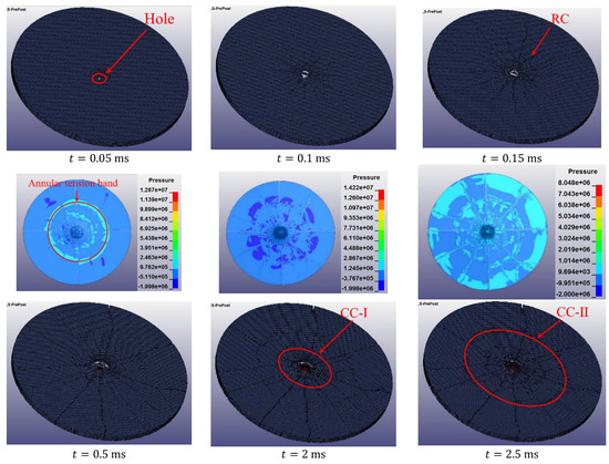
Figure 11.
Stress contour plot (top); and ice plate broken image (bottom) as the UEXB breaks the ice (the unit of pressure is “Pa”).
After the underwater detonation of TNT, the intense chemical reaction and the trend of bubble expansion generate an explosive shockwave. When the shockwave initially contacts the central lower surface of the ice plate, it generates higher radial and tangential pressure stresses as the shockwave propagates inside the ice plate in the form of a compression wave and contacts the back free surface (i.e., the upper surface of the ice plate in contact with air). Significant tensile waves are reflected due to the much lower acoustic impedance of air compared to ice. The compressive strength of the ice is much higher than its tensile strength; therefore, initial cracks often originate at the back free surface [53]. Throughout the entire icebreaking process, the ice plate continues to experience stress. When the deformation due to cohesive failure between finite element units exceeds a specified threshold, the units fail and are removed, resulting in the formation of cracks and holes.
From the stress contour, it is evident that a circular tensile stress zone formed around the hole, with radial and tangential tensile stresses radiating outward from the center. At , the tensile stress zone began to expand outward, and due to the radial tensile stress, radial cracks started to scatter outward from the center of the hole. At , due to the boundary effect of the original plate, shockwave reflections occurred at the edge of the ice sheet, resulting in a first-order circumferential tensile stress zone, causing the radial cracks to extend further outward from the initial cracks as the underwater explosive expanded continuously. At , a second-order circumferential tensile stress zone formed closer to the outer edge, and radial cracks extended all the way to the edge of the ice sheet due to the continuous action of these two tensile stress zones. At , first-order irregular circumferential cracks formed closer to the center, and subsequently, at , second-order irregular circumferential cracks formed closer to the outer edge. This is due to the initial splitting of the ice sheet caused by the compressive stress perpendicular to the ice sheet, followed by the influence of radial stress and upward longitudinal pressure, causing the inclined microcrack to slip [54]. After the formation of circumferential and radial cracks, the ice sheet was divided into different regions. The sections that had already fragmented and flipped upwards experienced compressive stress, while the parts that had not yet fractured continued to experience tensile stress.
Figure 12 displays a side-view contour and a lateral view of the ice sheet, the change in color of the bubbles and ice plates represents this change in pressure. Following the TNT detonation, when the shockwave contacted the lower surface, the ice sheet immediately developed fractures. As the shockwave propagated from the lower surface to the upper surface of the ice plate, stress waves reflected from the upper surface back to the lower surface. Because the ice sheet was in a free-floating state, the ice plate was collectively displaced upward under the influence of shockwaves and bubble action, resulting in the unloading of a portion of the shockwave. Consequently, the outward flipping of the ice mass from the central opening was not pronounced. The central region of the ice sheet exhibited an upward convex shape, corroborating the ice’s elastic–plastic characteristics. Influenced by the ice sheet’s discontinuities, the CGB no longer maintained a regular spherical shape but rather assumed an irregular, cone-like form at the upper end. As the gas bubbles further expanded, the CGB caused additional damage to the ice sheet, generating multiple circumferential cracks that penetrated from the bottom to the top. It can also be observed that when the shockwave became excessive, the ice sheet was more susceptible to developing radial cracks that penetrated from the top to the bottom. As the gas bubbles expanded upward, the ice was more likely to create circumferential pressure zones at the top of the ice sheet, leading to the formation of circumferential cracks that penetrated from the bottom to the top. From a lateral perspective, the expansion action of the UEXB caused the ice sheet to move upward by 0.6 mm, with a deflection of 2 mm at the center.
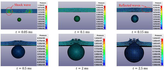
Figure 12.
Ice plate broken image and stress contour plot when the UEXB breaks the ice (left side-view of the ice sheet).
3.2.2. Damage to Ice by Compressed Gas Bubbles
Due to the limited clarity of the crack patterns in the stress contour, a top view of the ice plate without the pressure display is provided below the stress contour. To better observe the cracks, the ice plate was tilted at a 30° angle for observation, as shown in Figure 13.
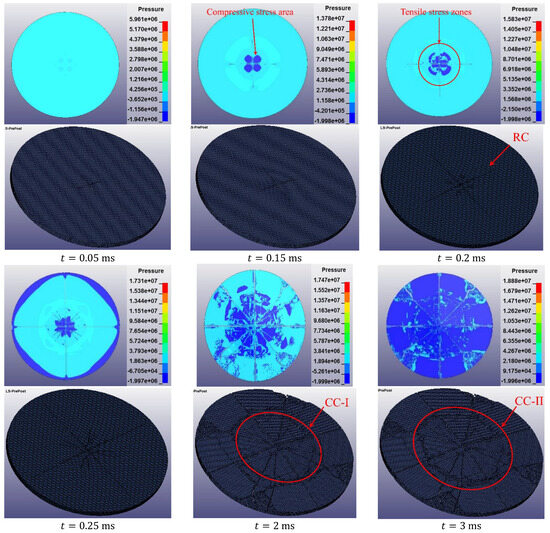
Figure 13.
Stress contour plot (top) and ice plate broken image (bottom) as the CGB breaks the ice (the unit of pressure is Pa).
When the CGB began to expand underwater, the shockwaves transmitted through the ice to the upper surface. The mechanism of load transmission was similar to that of the TNT underwater explosion. However, due to the relatively smaller shockwave generated by CGB, it did not create a significant hole in the ice plate.
At , compressive stress from the bottom of the ice plate was transmitted to the four corners of the radial crack center on the upper surface, forming a distinct compressive stress region. At , due to the influence of reflected tensile waves and tangential tensile stresses on the upper surface, a tensile stress zone formed at the edges of the radial crack. At , due to boundary effects, there was a shockwave reflection at the edges of the ice plate. Because the radial crack extended to the edge, there were four similar regions of reflected shockwaves. At , after the central region fractured, a compressive stress zone formed around the center of the ice plate, with a tensile stress zone at the edges. Finally, at , due to the complete splitting of the ice plate, the entire ice plate was subjected to compressive stress.
As shown in Figure 14, the damage mechanism of the CGB shockwave stage to the ice plate is similar to that of the UEXB shockwave stage. Because the CGB had a larger volume, the ice impeded the continuous expansion of the bubble. As the bubble continued to expand, the outer central region also rose; this resulted in continuous tensile stress in the upper part of the ice body. Cracks in the ice plate rapidly expanded, and circumferential cracks gradually appeared at the top. The lower part of the ice body experienced continuous compressive stress, causing the initial cracks formed during the shockwave phase under the ice plate to continue expanding, resulting in penetrating cracks. When the bubble reached its maximum volume, the ice plate moved upward by 0.6 mm as a whole, with a deflection of 6 mm at the top. This indicates that the continued expansion of the bubble is one of the main causes of the ice plate damage.
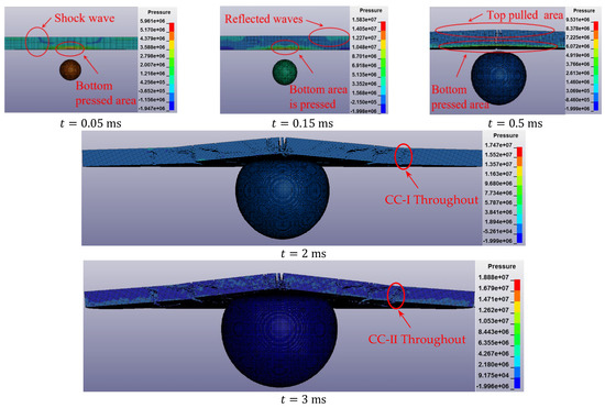
Figure 14.
Ice plate broken image and stress contour plot as the CGB breaks the ice (left side-view of the ice sheet).
3.2.3. Comparison of Ice Damage by Two Bubble Sources
As shown in Figure 15a, the damage inflicted by the UEXB on the ice plate ultimately manifests as radial cracks radiating from the center to the edge of the plate, multiple penetrating circumferential cracks centered around the perforation, and several tight circumferential cracks around the bottom perforation. This damage can be divided into three zones: the central perforation zone, with damage caused by the initial shockwave, primarily occurring in the central area of the perforation, resulting in penetrating cracks; the continuous tensile stress zone, with damage caused by the continuous upward expansion of the bubble, leading to the formation of a damage zone around the perforation due to continuous tensile stress; and the crack propagation zone, where cracks extend outward toward the edge, forming multiple circumferential cracks. Additionally, the ice fragments generated at the perforation site are relatively fine.
Figure 15.
Final damage caused by the (a) UEXB and (b) CGB to the ice plate.
As shown in Figure 15b, the CGB does not cause significant large holes on the ice plate, but eventually presents radial through-radial cracks from the center to the edge of the ice plate, and circumferential cracks with the center of the ice plate as the center of the circle, forming large sustained tensile stress zone damage caused by the continuous upward development of bubbles, and a crack expansion zone developing toward the outer edge. Due to the small shockwave load, the damaged block of the ice slab is larger under the load of continuous bubble development.
Following the conclusion of the initial shockwave, the bubble rapidly expanded, with the ice plate hindering the bubble’s development. Due to the continuous expansion of the bubble, the central region of the ice plate was pushed up by the bubble and continued to expand until the bubble stopped expanding. During the continued expansion of the bubble, CGB induced greater deflection and deformation in the ice plate, resulting in a larger area of crack formation.
As shown in Figure 16a, after the first shockwave caused damage to the ice plate, the ongoing development of the bubbles continued to cause observable damage to the ice plate. Due to the larger volume of CGB compared to UEXB, the tensile stress effects caused by CGB’s continued upward development on the ice were more pronounced, and the ratio of failed elements caused by CGB is higher than that of UEXB. Five working condition studies with different energy levels for both bubble sources were conducted, resulting in the ratio of failed numbers curves shown in Figure 16b. It can be observed that the number of failed elements caused by CGB remains consistently higher than that caused by UEXB.
Figure 16.
Comparison of the ratio of failure units caused by two kinds of bubbles at different energies to the ice plate: (a) the ratio of different stages failed elements curve; and (b) the ratio of total failed elements curve.
3.2.4. Optimum Standoff Distance
To use the energy of bubbles more reasonably and avoid waste, it is of great significance to explore the optimal burst distance. This section uses two bubble sources with the same energy of 120 J, explores the damage characteristics of the ice plate under the action of two bubble sources with different distances, and realizes this purpose by detecting the final number of failed particles of the ice plate.
Figure 17 shows the curve of the ratio of failed elements under different standoff distances. The ratio of failed units increases initially and then decreases as the distance increases. The optimal distance for icebreaking was not the closest and not the farthest distance between the bubble and the ice because the effect of the two bubbles on the ice plate is complex. The UEXB mainly relied on the shockwave on the ice plate damage, the shockwave was generated by the need for an appropriate distance to achieve the best destructive effect. A distance that is too small will lead to the shockwave not fully developing, and a distance that is too large will lead to a shockwave in the water attenuation that is too large [23]. The CGB mainly relied on shockwaves and the bubble expansion effect on the ice plate damage. When the distance is too small, the ice plate limits the development of the bubble morphology, and when the distance is too large, it leads to the attenuation of the shockwave and the expansion of the bubble’s effect. The optimal detonation distance primarily differs between the UEXB and CGB due to the different mechanisms of icebreaking that each relies on. Therefore, choosing a more suitable detonation distance for bubble icebreaking operations can yield better icebreaking results. Under the condition that the inner energy of the bubble is 120 J, for an ice plate with a radius of 0.19 m and a thickness of 0.15 m, the optimum standoff distance of the compressed gas bubble with 120 J is 0.03 m, and the optimum standoff distance of the TNT with 120 J is 0.02875 m.
Figure 17.
The time–number of failed elements curve.
4. Conclusions
This paper introduces a two-way coupling numerical model of ice–water–gas based on the ALE method. The reliability of this numerical model was validated through comparisons with experiments. Furthermore, a comparative analysis of the effects of a TNT underwater explosion and CGB on ice plates was conducted. The following conclusions were drawn:
- (1)
- When the initial internal energies of the two bubbles are the same, the CGB has a larger maximum volume than the UEXB, and its period is longer. The UEXB generates a larger shockwave and dissipates more energy. Since this study focuses on near-wall conditions, under the same internal energy conditions, the UEXB’s collapse produces a higher peak jet velocity than the CGB, and the jet duration and secondary shockwave are both shorter than the CGB. This is related to the development of bubbles near the wall.
- (2)
- Due to the larger shockwave generated by the UEXB under the same energy conditions, the UEXB is more likely to create a hole in the ice sheet. The CGB causes a larger damaged area on the ice sheet, and its expansion process has a more pronounced effect on ice sheet damage, resulting in larger ice fragments compared to the UEXB. This is related to the different ways in which the UEXB and CGB damage the ice. Moreover, under the same energy conditions, the total number of failure elements caused by the CGB on the ice sheet is higher than that of the UEXB, indicating an overall better icebreaking effect for the CGB. Additionally, the CGB generates a smaller shockwave, making it a safer option for practical operational scenarios.
- (3)
- The choice of the optimal braking distance is an important issue in practical icebreaking applications. It involves many factors such as the nature of the ice, the characteristics of the bubbles, and boundary conditions. For the parameter of the blast distance discussed in this paper, a smaller blast distance does not necessarily guarantee better icebreaking effects. Further research on this issue will involve more parameters and considerations. For an ice plate with a radius of 0.19 m and a thickness of 0.15 m, the optimum standoff distance of the compressed gas bubble with 120 J is 0.03 m, and the optimum standoff distance of the TNT with 120 J is 0.02875 m.
Author Contributions
Conceptualization, Z.Y. and Q.W.; Data curation, Z.Y.; Funding acquisition, Q.W. and Y.X.; Methodology, Z.Y., B.-Y.N. and Q.W.; Resources, Q.W. and Y.X.; Software, Z.W.; Supervision, Q.W.; Writing—original draft, Z.Y. and Q.W.; Writing—review and editing, P.L. and Y.X. All authors have read and agreed to the published version of the manuscript.
Funding
This work is supported by the National Natural Science Foundation of China (Nos. 52192693, 52192690, 52371270 and U20A20327), and the National Key Research and Development Program of China (2021YFC2803400), for which the authors are most grateful.
Institutional Review Board Statement
Not applicable.
Informed Consent Statement
Not applicable.
Data Availability Statement
There are no publicly available data for this study.
Conflicts of Interest
The authors declare no conflict of interest.
Abbreviations
| UEXB | Underwater Explosion Bubble |
| CGB | Compressed Gas Bubble |
| RC | Radical Crack |
| CC | Circumferential Crack |
| CC-1 | First Circumferential Crack |
| CC-2 | Second Circumferential Crack |
References
- Sazonov, K.; Dobrodeev, A. Ice Resistance Assessment for a Large Size Vessel Running in a Narrow Ice Channel Behind an Icebreaker. J. Mar. Sci. Appl. 2021, 20, 446–455. [Google Scholar] [CrossRef]
- Ni, B.Y.; Chen, Z.W.; Zhong, K.; Li, X.A.; Xue, Y.Z. Numerical simulation of a polar ship moving in level ice based on a oneway coupling method. J. Mar. Sci. Eng. 2020, 8, 692. [Google Scholar] [CrossRef]
- Du, Y.; Sun, L.P.; Pang, F.Z.; Li, H.C.; Gao, C. Experimental research of hull vibration of a full-scale river icebreaker. J. Mar. Sci. Appl. 2020, 19, 182–194. [Google Scholar] [CrossRef]
- Ni, B.Y.; Wang, Q.; Xue, Y.Z.; Wang, Y.; Wu, Q.G. Numerical simulation on the damage of ice floe by high-pressure bubble jet loads. In Proceedings of the Workshop and Symposium on Safety and Integrity Management of Operations in Harsh Environments, St. John’s, NL, Canada, 15–17 July 2019. [Google Scholar]
- Ni, B.Y.; Pan, Y.T.; Yuan, G.Y.; Xue, Y.Z. An experimental study on the interaction between a bubble and an ice floe with a hole. Cold Reg. Sci. Technol. 2021, 187, 103281. [Google Scholar] [CrossRef]
- Cui, P.; Zhang, A.M.; Wang, S.; Khoo, B.C. Ice breaking by a collapsing bubble. J. Fluid Mech. 2018, 841, 287–309. [Google Scholar] [CrossRef]
- Kan, X.Y.; Zhang, A.M.; Yan, J.L.; Wu, W.B.; Liu, Y.L. Numerical investigation of ice breaking by a high-pressure bubble based on a coupled BEM-PD model. J. Fluids Struct. 2020, 96, 103016. [Google Scholar] [CrossRef]
- Yuan, G.Y.; Ni, B.Y.; Wu, Q.G.; Xue, Y.Z.; Zhang, A.M. An experimental study on the dynamics and damage capabilities of a bubble collapsing in the neighborhood of a floating ice cake. J. Fluids Struct. 2020, 92, 102833. [Google Scholar] [CrossRef]
- Jorgensen, J.K.; Gyselman, E.C. Hydroacoustic measurements of the behavioral response of arctic riverine fishes to seismic airguns. J. Acoust. Soc. Am. 2009, 126, 1598–1606. [Google Scholar] [CrossRef]
- Nikolaev, S.E. Cutting Sea Ice by Directed Blasting (Opyt Razrusheniya Morskogo lda Napravlennym Vzryovom); Cold regions research and engineering laboratory: Hanover, NH, USA, 1973. [Google Scholar]
- Mellor, M. Breaking Ice with Explosives; Cold Regions Research & Engineering Laboratory, US Army Corps of Engineers: Hanover, NH, USA, 1982; p. 3. [Google Scholar]
- Mellor, M. Derivation of guidelines for blasting floating ice. Cold Reg. Sci. Technol. 1987, 13, 193–206. [Google Scholar] [CrossRef]
- Wang, Y.; Qin, Y.Z.; Yao, X.L. A combined experimental and numerical investigation on damage characteristics of ice sheet subjected to underwater explosion load. Appl. Ocean. Res. 2020, 103, 102347. [Google Scholar] [CrossRef]
- Mellor, M. Breakage of Floating Ice by Compressed Gas Blasting; Industrial Laboratory (USSR): Moscow, Russia, 1972. [Google Scholar]
- Zhang, A.M.; Yao, X.L.; Li, J. The interaction of an underwater explosion bubble and an elastic–plastic structure. Appl. Ocean. Res. 2008, 30, 159–171. [Google Scholar] [CrossRef]
- Zhang, A.M.; Wang, S.P.; Huang, C.; Wang, B. Influences of initial and boundary conditions on underwater explosion bubble dynamics. Eur. J. Mech. B/Fluids 2013, 42, 69–91. [Google Scholar] [CrossRef]
- Li, S.; Zhang, A.M.; Han, R.; Liu, Y.Q. Experimental and numerical study on bubble-sphere interaction near a rigid wall. Phys. Fluids 2017, 29, 092102. [Google Scholar] [CrossRef]
- Zhang, A.; Li, S.M.; Cui, P.; Li, S.; Liu, Y.L. A unified theory for bubble dynamics. Phys. Fluids 2023, 35, 033323. [Google Scholar] [CrossRef]
- Cui, P.; Zhang, A.M.; Wang, S.P.; Liu, Y.L. Experimental study on interaction shock wave emission and ice breaking of two collapsing bubbles. J. Fluid Mech. 2020, 897, A25. [Google Scholar] [CrossRef]
- Wu, Q.G.; Wang, Z.C.; Ni, B.Y.; Yuan, G.Y.; Semenov, Y.A.; Li, Z.Y.; Xue, Y.Z. Ice-Water-Gas Interaction during Icebreaking by an Airgun Bubble. J. Mar. Sci. Eng. 2022, 10, 1302. [Google Scholar] [CrossRef]
- Zhou, P.; Zhu, S. Mechanism analysis of ice damage under underwater near-field explosion. Inter-Noise Noise-Con Congr. Conf. Proc. 2019, 259, 647–658. [Google Scholar]
- Zhang, W.; Shi, D.; Feng, B.; Liu, T. Analysis of meso-mechanism of ice damage under two loads of underwater explosion. In Proceedings of the International Conference on Mechanical Design and Simulation (MDS 2022), Wuhan, China, 18–20 March 2022. [Google Scholar]
- Wang, Y.; Qin, Y.Z.; Wang, Z.K.; Yao, X.L. Numerical study on ice damage characteristics under single explosive and combination explosives. Ocean. Eng. 2021, 223, 108688. [Google Scholar] [CrossRef]
- Wang, Y.; Yao, X.L.; Qin, Y.Z. Investigation on influence factors about damage characteristics of ice sheet subjected to explosion loads: Underwater explosion and air contact explosion. Ocean. Eng. 2022, 260, 111828. [Google Scholar] [CrossRef]
- Liu, J.H.; Wu, Y.; Zhao, B.L. Dynamic Response of FRP Structure under Underwater Explosion Shock Wave. Ship Mech. 2000, 3, 51–58. [Google Scholar]
- An, F.J.; Shi, H.J.; Liu, Q. Near-field pressure characteristics of underwater explosion and its fluid-structure interaction with structure. J. Ordnance Ind. 2015, 36, 13–24. (In Chinese) [Google Scholar]
- L.S. Technology. LS-DYNA Keyword User’s Manual; L.S. Technology: Driffield, UK, 2020. [Google Scholar]
- Zhang, T.T. Study on Protection Characteristics of Ship Side Structure and Equipment under Underwater Contact Explosion. Master’s Thesis, Harbin Engineering University, Harbin, China, 2017. (In Chinese). [Google Scholar]
- Green, L.; Lee, E.; Mitchell, A.; Tipton, R.; van Thiel, M.; Finger, M. UCRL-89664 CA; Lawrence Livemore National Laboratory: Livermore, CA, USA, 1993. [Google Scholar]
- Ralph, M. LA-UR-15-29536; Los Alamos National Laboratory: Los Alamos, NM, USA, 2015. [Google Scholar]
- Khalifa, Y.A.; Lotfy, M.N.; Fathallah, E. Effectiveness of Sacrificial Shielding for Blast Mitigation of Steel Floating Pontoons. J. Mar. Sci. Eng. 2023, 11, 96. [Google Scholar] [CrossRef]
- Alia, A.; Souli, M. High explosive simulation using multi-material formulations. Appl. Therm. Eng. 2006, 26, 1032–1042. [Google Scholar] [CrossRef]
- Hallquist, J.O. LS-DYNA Keyword User’s Manual; Livermore Software Technology Corporation: Livermore, CA, USA, 2007; Volume 970, pp. 299–800. [Google Scholar]
- Liu, W.T.; Ming, F.R.; Zhang, A.M.; Miao, X.H.; Liu, Y.L. Continuous simulation of the whole process of underwater explosion based on Eulerian finite element approach. Appl. Ocean. Res. 2018, 80, 125–135. [Google Scholar] [CrossRef]
- Anghileri, M.; Castelletti, L.M.; Invernizzi, F.; Mascheroni, M. A survey of numerical models for hail impact analysis using explicit finite element codes. Int. J. Impact Eng. 2005, 31, 929–944. [Google Scholar] [CrossRef]
- Kim, H.; Welch, D.A.; Kedward, K.T. Experimental investigation of high velocity ice impacts on woven carbon/epoxy composite panels. Compos. Part A Appl. Sci. Manuf. 2003, 34, 25–41. [Google Scholar] [CrossRef]
- Kim, J.H.; Shin, H.C. Application of the ALE technique for underwater explosion analysis of a submarine liquefied oxygen tank. Ocean. Eng. 2008, 35, 812–822. [Google Scholar] [CrossRef]
- Klaseboer, E.; Hung, K.C.; Wang, C.; Wang, C.W.; Khoo, B.C.; Boyce, P.; Debono, S.; Charlier, H. Experimental and numerical investigation of the dynamics of an underwater explosion bubble near a resilient/rigid structure. J. Fluid Mech. 2005, 537, 387–413. [Google Scholar] [CrossRef]
- Cole, R.H. Underwater Explosion; Princeton University Pass: Princeton, NJ, USA, 1948. [Google Scholar]
- Li, X.Y.; Ding, H.J.; Chen, W.Q. Axisymmetric elasticity solutions for a uniformly loaded annular plate of transversely isotropic functionally graded materials. Acta Mech. 2008, 196, 139–159. [Google Scholar] [CrossRef]
- Rabczuk, T. Computational methods for fracture in brittle and quasi-brittle solids: State-of-the-art review and future perspectives. Int. Sch. Res. Not. 2013, 2013, 849231. [Google Scholar] [CrossRef]
- Seagraves, A.N.; Radovitzky, R.A. An analytical theory for radial crack propagation: Application to spherical indentation. J. Appl. Mech. 2013, 80, 041018. [Google Scholar] [CrossRef]
- Yuan, G.Y.; Ni, B.Y.; Wu, Q.G.; Xue, Y.Z.; Han, D.F. Ice breaking by a high-speed water jet impact. J. Fluid Mech. 2022, 934, A1. [Google Scholar] [CrossRef]
- Zhang, A.M. Study on Three-Dimensional Dynamic Characteristics of Underwater Explosion Bubbles. Ph.D. Thesis, Harbin Engineering University, Harbin, China, 2006. (In Chinese). [Google Scholar]
- Zong, Z.; Zhao, Y.J.; Zou, L. Numerical Calculation of Damage to Underwater Explosive Structures; Science Press: Beijing, China, 2014. (In Chinese) [Google Scholar]
- Li, J.; Rong, J.L.; Xiang, D.L. Numerical study of bubble motion by underwater explosion near free surface. Eng. Mech. 2011, 27, 200–205. [Google Scholar]
- An, F.J.; Wu, C.; Wang, N.F. A Research on the Energy Dissipation of Underwater Explosion. Trans. Beijing Inst. Technol. 2011, 4, 379–382. [Google Scholar]
- Gong, S.W.; Ohl, S.W.; Klaseboer, E.; Khoo, B.C. Scaling law for bubbles induced by different external sources: Theoretical and experimental study. Phys. Rev. E 2010, 81, 056317. [Google Scholar] [CrossRef] [PubMed]
- Cooper, P.W. Explosives Engineering; John Wiley & Sons: Hoboken, NJ, USA, 2018. [Google Scholar]
- Lauterborn, W.; Bolle, H. Experimental investigations of cavitation-bubble collapse in the neighborhood of a solid boundary. J. Fluid Mech. 1975, 72, 391–399. [Google Scholar] [CrossRef]
- Lauterborn, W. Cavitation bubble dynamics-New tools for an intricate problem. Appl. Sci. Res. 1982, 38, 165–178. [Google Scholar] [CrossRef]
- Li, S.; Zhang, A.M.; Han, R. Study on the formation mechanism and loading characteristics of water jet of high-pressure pulsating bubbles in water. Chin. J. Theor. Appl. Mech. 2019, 51, 1666–1681. (In Chinese) [Google Scholar]
- Petrenko, V.F.; Whitworth, R.W. Physics of Ice; Oxford University Press: Oxford, UK, 1999. [Google Scholar]
- Nguyen, H.; Pathirage, M.; Rezaei, M.; Issa, M.; Cusatis, G.; Bažant, Z.P. New perspective of fracture mechanics inspired by gap test with crack-parallel compression. Proc. Natl. Acad. Sci. USA 2020, 117, 14015–14020. [Google Scholar] [CrossRef]


Disclaimer/Publisher’s Note: The statements, opinions and data contained in all publications are solely those of the individual author(s) and contributor(s) and not of MDPI and/or the editor(s). MDPI and/or the editor(s) disclaim responsibility for any injury to people or property resulting from any ideas, methods, instructions or products referred to in the content. |
© 2023 by the authors. Licensee MDPI, Basel, Switzerland. This article is an open access article distributed under the terms and conditions of the Creative Commons Attribution (CC BY) license (https://creativecommons.org/licenses/by/4.0/).