Abstract
Shellfish reefs around the world have become degraded, and recent efforts have focused on restoring these valuable habitats. This study is the first to assess the efficacy of a bouchot-style reef, where mussels were seeded onto wooden stakes and deployed in a hypereutrophic estuary in Australia. While >60% of translocated mussels survived one month, after ten months, only 2% remained alive, with this mortality being accompanied, at least initially, by declining body condition. Mussel survival, growth, body condition and recruitment were greater on the top section of the stake, implying that the distance from the substrate was important. More fish species inhabited the reefs (31) than unstructured control sites (17). Reefs were also colonised by a range of invertebrate species, including 11 native and six non-indigenous species. However, the number of individuals declined from 4495 individuals from 14 species in December 2019 to 35 individuals representing 4 species in March 2021, likely due to hypoxic bottom water conditions following unseasonal rainfall. Although the bouchot-style reefs were unable to sustain mussels and other invertebrates over sequential years, this approach has the potential to be successful if deployed in shallow water or intertidal zones, which are largely exempt from biotic and abiotic stressors characteristic of deeper waters in microtidal estuaries.
1. Introduction
As climate change continues to exacerbate the effects of anthropogenic impacts across global land and seascapes, restoration practitioners seek new and novel approaches to restore ecosystem functioning in degraded habitats [1,2]. Among the numerous aquatic systems that require restoration interventions, temperate estuaries, largely through excessive nutrient input, are the most degraded of all marine ecosystems [3]. This is particularly true for those estuaries that have been the foci for human expansion, resulting in extensive modifications to catchments for agriculture, industry and other human developments including the expansion of ports, leading to the introductions of non-indigenous species (NIS) and the loss of important biogenic habitats, such as shellfish reefs [4,5,6,7].
Shellfish reefs, comprising mussels and oysters, were once commonplace in temperate estuaries throughout the world but were largely lost or degraded through a range of anthropogenic influences, including declining water quality, disease, and overharvesting for food and construction material [4,5]. As shellfish reefs provide a multitude of ecosystem services, shellfish reef restoration projects have accelerated in the last decade, and this includes the use of artificial hard structures to provide suitable habitat for larval settlement [4,5,6]. For example, in lieu of natural oyster shell, restoration in Chesapeake Bay after 5 years concrete modular reefs deployed subtidally (7 m depth) were found to contain >8000 mussels m−2 of surface area [6]. The addition of hard substrates has also been employed in temperate regions of Australia, where large-scale restoration efforts have occurred at over 40 locations since 2015 [8].
In addition to shoreline erosion protection during storms and their enormous water filtration capacity, shellfish reefs also support fishery production through the provision of habitat and food resources [9,10]. This is particularly important in estuaries, which largely comprise unstructured soft sediments, with the protrusion of the three-dimensional hard structure interspersed with interstitial spaces, of variable sizes, providing a predator refuge. Thus, shellfish reefs often support greater fish densities than unstructured habitats [11]. The three-dimensional structures also promote the settlement, growth and survival of shellfish and other filter feeders by providing better access to feeding opportunities. The elevation provides a buffer zone from the sediment–water interface where oxygen concentrations are typically lower and also reduces exposure to benthic detritus that can become resuspended by waves [12,13,14,15]. As seston derived from resuspension can contain high concentrations of silt and is thus of low quality for suspension feeders, it can lead to increased processing costs (pseudofeces production) and low absorption efficiencies and thus reduced survival [7,16,17]. For example, the condition of the Horse Mussel Atrina zelandica was found to decrease after exposure to elevated sediment concentrations after three days and their natural distribution was governed by suspended sediment loads [17]. The habitat heterogeneity provided by the reefs also promotes biodiversity primarily through the presence of structurally complex microhabitats, comprising matrices of living shellfish, shells and sediment, which support a diverse range of invertebrate species [18,19]. For example, beds of the Mediterranean Mussel Mytilus galloprovincialis in South Africa were found to support a rich assemblage of 80 macroinvertebrate species [20].
Restoration initiatives are particularly appropriate for estuaries in south-western Australia as these systems have been heavily modified since European settlement [21,22]. However, this region is also recognised as a global warming and drying hotspot [23], where sea surface temperatures have increased at a faster rate (0.1–0.3 °C per decade) than 90% of the ocean globally [24], and rainfall declines have been among the most pronounced of any Australian region [25,26,27]. The effects of these modifications have been particularly apparent in the microtidal Swan-Canning Estuary, which flows through Western Australia’s capital city, Perth [28].
The Swan-Canning Estuary is among the most extensively modified estuary in Western Australia and was recognised as one of the most hypereutrophic of 131 estuaries and coastal ecosystems examined globally by Cloern et al. [29]. The estuary comprises an upper riverine region (the Swan and Canning rivers), a large central basin and an entrance channel, which has been widened and deepened to facilitate Western Australia’s largest and busiest container port. The presence of the port accounts for the estuary containing 46 of the States’ 60 marine NIS (non-indigenous species) [30]. The basin of the Swan-Canning Estuary also once supported reefs of the native Flat Oyster Ostrea angasi, as was evident from the banks of shell removed in the first half of the twentieth century [22]. While the only remaining shellfish in high abundance is M. galloprovincialis, the larvae of this species has a preference to settle on hard structures, which are now non-existent in deeper water.
The declines in streamflow and increased seawater intrusion have led to salinities in bottom waters throughout the basin of the Swan-Canning Estuary remaining close to seawater (e.g., 32–37) throughout the year [31]. This is particularly the case during ‘dry years’ when annual rainfall is below average (759 mm), which has occurred in 15 out of the 20 years prior to 2022 [32]. While the increased marinization of the estuary has resulted in habitat compression of estuarine species upstream, such as the Black Pygmy Mussel Xenostrobus securis, it has also provided a more stable saline environment for species with marine affinities [31,33]. The estuary has also had a long history of hypoxia (<2 mg L−1 of dissolved oxygen), particularly in the bottom waters of the upper riverine region, causing major impacts for fish and invertebrate fauna [28,34]. During ‘wet years’, however, when rainfall is above (or approaches) average, the water column in the estuary basin can become stratified and a hypoxic zone can persist in bottom waters for several weeks at the time [35].
Large-scale shellfish reef construction projects in Australia have typically involved the deployment of a limestone reef base, which elevates the shellfish off the typically soft and low oxygen bottom waters [8]. While shellfish reef restoration has largely focused on hatchery-sourced oysters (Saccostrea glomerata and/or Ostrea angasi), M. galloprovincialis, which in Australia comprises both northern and southern hemisphere halotypes [36], has been receiving increased attention [7,8]. Furthermore, as mytilid mussels continue to produce byssal threads throughout their life, if dislodged, they can reattach to new structures.
Mytilids are an important commercial aquaculture species and a range of approaches have been employed to maximise harvests [37]. These typically involve suspending the mussels in the water column to provide better feeding opportunities and less burial from sediments as well as to reduce mortality from benthic predators, such as crabs and rays [38]. While the use of longlines or raft cultures, where ropes are suspended from the surface, are more typical to facilitate these requirements, a style of farming developed on the French Atlantic coast, referred to as bouchot (shellfish bed) farming, employs mussels grown on wooden poles staked into the substrate. Although the protrusion of wooden poles from the benthos may not appear natural, these structures, which will decompose over time, have the potential to form the foundations of shellfish reefs; thus, this type of approach is potentially transferable as a restoration option.
The aim of this study was to assess the efficacy of bouchot-style reefs as a restoration option for M. galloprovincialis in the Swan-Canning Estuary. This was undertaken by quantifying the performance of translocated M. galloprovincialis (growth, body condition and survival) on three constructed bouchot reefs, the presence of newly recruited M. galloprovincialis and an assessment of the fish and invertebrate species that colonised these habitats. The results of this study are of interest to environmental managers and will assist shellfish reef practitioners in assessing appropriate approaches and locations for future shellfish reef restoration projects.
2. Materials and Methods
2.1. Study Location
The Swan-Canning Estuary (32.0° S and 115.9° E) in south-western Australia is ~50 km long, has a surface area of ~55 km2, and remains permanently open to the Indian Ocean (Figure 1) [20]. Although most of the estuary is shallow (<2 m in depth), it reaches a maximum depth of ~20 m in the entrance channel, and up to ~17 m in the main basin. The composition of the sediment differs markedly between the shallow marginal shoals (<2 m deep) and the deeper waters (>2 m deep). Nearshore substrates contain a greater proportion of medium-grain-size sand than the offshore sediments, which comprise higher percentages of particulate organic matter and finer inorganic particles (i.e., silt and fine sand) [39].
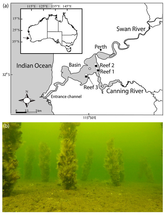
Figure 1.
(a) Map of Swan-Canning Estuary showing three locations of the bouchot-style Mytilus galloprovincialis reefs (filled rectangles) constructed in 2019, the RUV control sites (open rectangles) and the water quality monitoring site (open circle) and (b) photograph showing one of the reefs several months after deployment.
South-western Australia experiences a Mediterranean climate [23], with warm, dry summers and cool, wet winters, and ~80% of the annual rainfall occurs between June and September. This highly seasonal rainfall pattern, combined with the microtidal tidal regime of the Swan-Canning Estuary (tidal range < 2 m), results in marked seasonal variations in water physical–chemical conditions in this salt-wedge estuary [33]. Salinities are typically stable and relatively high throughout much of the estuary basin during the austral summer (December to February), but during winter, may vary markedly along the estuary following substantial freshwater discharge [33], leading to marked stratification of the water column and hypoxia [28,33].
The Swan-Canning Estuary and its catchment have been heavily modified since European settlement and contains the City of Perth, the capital of Western Australia (~2 million people). Such modifications include substantial land clearing for urbanization and agriculture, hardening of shorelines, blasting and dredging of the mouth of the estuary to permanently connect it to the ocean and allow the construction of Fremantle Port [21]. As such, the system was categorised as “extensively modified” in an audit of the condition of ~1000 estuaries across Australia [40].
2.2. Environmental Variables
Long-term average monthly rainfall (1944–2023) and total monthly rainfall (2019–2023) recorded at Perth Airport (Station 009021) were extracted from the Australian Government Bureau of Meteorology (2023) database [31]. Long-term average monthly streamflow (1970–2023) and total monthly streamflow (2019 and 2023) recorded for the Swan River (Station 616011) were extracted from the Water Information Reporting (WIR) database [41]. Weekly values (2019–2023) for water temperature, salinity and dissolved oxygen concentration at the surface (0.5 m depth) and bottom of the water column (6.0 m depth) recorded at Heathcote (site 6161869; Figure 1) were also extracted from the WIR database [41].
2.3. Reef Construction and Sampling Regime
Individuals of M. galloprovincialis (shell length 40–70 mm, 0+ age class) were collected from mooring ropes in the entrance channel of the Swan-Canning Estuary, and their external epibionts were removed by a combination of aerial exposure and manual agitation. Three liters of M. galloprovincialis was then used to seed the top 1 m of each of 300 wooden (jarrah; Eucalyptus marginata) stakes (1500 (H) × 25 (W) × 25 (D) mm). For this, a PCV pipe was used to apply a commercial cotton sock around the mussels on each stake. Thus, the use of established mussels negated the use of coconut fibre ropes to collet spat, as is used in traditional bouchot culture. Instead, this study employed a similar process to that used in commercial aquaculture where established mussels are reattached to grow-out ropes at a desired density that promotes growth, and this has been highly successful for food production.
The collection and socking of mussels onto the stakes were undertaken over three consecutive weekends and involved community volunteers. On each weekend between late March and early April 2019, 100 stakes were deployed at 3 locations in the main basin of the Swan-Canning Estuary (Figure 1). The reefs were constructed in ~4 m depth by SCUBA divers hammering the stakes ~0.5 m into the substrate approximately 1 m apart in a grid pattern covering an area of ~100 m2. These sites were selected based on their depth, with 3 m being the minimum vertical clearance allowed for structures in navigable waters, and their requirement to be located outside of recreational zones and marine parks.
Three stakes were retained at the time of deployment and a further three stakes were removed each month from each of the three reefs by snorkelling until February 2020, with a further three stakes collected from each reef in March 2021 and January 2023. Stakes were individually placed in large plastic bags, which were sealed and transported to the laboratory, where the above substrate portion of each stake was divided into three ~300 mm sections, with the top of the stake between 700 and 1000 mm from the sediment, the middle section 350 to 650 mm from the sediment and the bottom section of the stake 0 to 300 mm from the sediment. For each stake and section, each M. galloprovincialis was counted, its shell length measured to the nearest 0.5 mm using vernier callipers and its tissue removed and dried at 60 °C for 72 h or until a constant dry weight was reached. These samples were employed to explore patterns in growth, recruitment, body condition and survival.
Fish assemblages at the reef sites and adjacent unstructured control sites, located 0.5–1 km away (Figure 1) were monitored using Remote Underwater Videos (RUVs) in accordance with Animal Ethics Permit O2996/17. RUVs were chosen over baited systems as the spread of the bait plume has the potential to attract fish from outside of the reef area and, thus, those fish that are not using the reef directly. Each RUV comprised a camera (GoPro Hero 2018; GoPro, Inc. San Mateo, CA, USA) attached to a weighted rectangle steel frame (340 mm in height and 310 × 310 mm in length and width) and lowered to the substrate. All footage was recorded at a resolution of 1920 × 1080 pixels at 60 frames s−1 and for at least one hour.
In each month between October 2018 and June 2020 (except for January, March and October 2019), one RUV was deployed at each reef and adjacent control site. On each sampling occasion, one of the three reefs was chosen at random and a second deployment was conducted. RUV videos were collected prior to the deployment of the reefs (October 2018 to February 2019) to determine whether there were any underlying differences in the characteristics of the fish fauna among site and then post-deployment (April 2019 to June 2020) to investigate differences between the habitats.
The relative abundance of each fish and large crustacean species, e.g., Blue Swimmer Crabs (Portunus armatus), which is a key recreationally targeted species [42], was determined by counting the maximum number of individuals (MaxN) of each species in each frame commencing from the moment the RUV frame hit the benthos and continuing for 60 min [43]. Each of the taxa recorded was allocated to a number of functional guilds, i.e., estuarine usage, feeding mode and habitat (Table A1), following the rationale given by [44,45].
The invertebrates directly attached to the stakes and their associated epibiont community were removed from the top section of each stake (where they were most abundant), from samples in May, June, September and December 2019, and March 2021 and January 2023. Each sample was wet sieved using a 2000 μm mesh, and the invertebrates were stored in a 70% ethanol solution. Invertebrates were then separated from any material and sediment retained from the sieving and subsequently enumerated and identified to their lowest taxonomic level.
2.4. Statistical Analyses
The growth patterns of M. galloprovincialis were initially explored using traditional and seasonally adjusted von Bertalanffy growth models. While the seasonally adjusted provided a better fit (p < 0.001), the model still yielded low R2 values when applied to each reef, i.e., R2 = 0.18–0.73. Instead, as all translocated M. galloprovincialis were assumed to be the same age on each sampling occasion, shell length (mm) differences among reefs and stake sections in each month were analysed using Analysis of Variance (ANOVA). The assumption that all mussels belonged to the same cohort was consistent with the shell lengths in the adjoining embayment of Cockburn Sound where this species is grown commercially and spat collection ropes are replaced each year, the location of the mussels towards the top of the mooring ropes and, compared to the larger mussels that were present, largely lacked biofouling.
The body condition of M. galloprovincialis was explored using the relationship between soft tissue dry mass and shell length, an approach used in previous assessment of bivalve condition (e.g., [46,47]). To facilitate comparisons among month, reef site and stake section Analysis of Covariance (ANCOVA) was employed, which standardised for shell length (to the mean value 61 mm) to help account for spatial and temporal differences in shell length. Prior to analyses, data for shell length and dry mass were log transformed. Shell length and body condition data were analysed using IBM SPSS (Version 28.0).
The MaxN of each species in each replicate RUV sample was used to construct a data matrix and calculate the number of species and total MaxN in each sample. The data for these two univariate variables were examined using a Draftsman plot, to visually assess if the distribution of values were skewed and, if so, the transformation required to ameliorate this effect. This showed that total MaxN required a fourth-root transformation. The data for both variables before and after the deployment of the bouchot-style reefs were used to construct four Euclidean distance matrices. In turn, each was subjected to a two-way univariate Permutational Multivariate Analysis of Variance (PERMANOVA) [48] test to determine whether they varied significantly (p < 0.05) with Habitat (two levels; reef and control) and Time (two levels; pre-deployment, i.e., October-December 2018 and February 2019 or post-deployment, i.e., the 14 months between April 2019 and June 2020).
The data matrix of the MaxN abundance of each species in each replicate sample was divided to separate those samples collected at each site before and after the deployment of the bouchot-style reefs. The data in each matrix were dispersion-weighted [49] to down-weight the abundances of heavily-schooling species whose numbers were erratic, relative to those that return more consistent values, and then square-root transformed to balance the contributions of relatively abundant species, compared to those with lower MaxN values [50]. The transformed data in each matrix were then used to construct a Bray–Curtis resemblance matrix. These were separately subjected to the same two-way PERMANOVA design above. If required, post hoc testing was conducted using pairwise PERMANOVA.
Trends in the fish faunal community data were explored using a range of multi-dimensional scaling (MDS) approaches and Canonical Analysis of Principal coordinates (CAP) [50]. The averages of repeated bootstrap samples (bootstrapped averages) were used to construct a mMDS ordination plots for the main effects of Habitat and, if significantly different, also Time. Superimposed on to each plot were points representing the group average (i.e., the average of the bootstrapped averages) and the associated, smoothed and marginally bias-corrected 95% bootstrap region, in which 95% of the bootstrapped averages fall [51]. Note that the Time factor for the post-deployment analyses contained 14 levels, which, for clarity, was too complex to show on a bootstrapped mMDS plot and so was visualised using a centroid nMDS ordination. The same Bray–Curtis resemblance matrix was used to create a distance among centroids matrix, which was, in turn, used to generate a nMDS ordination plot [52]. A CAP ordination plot was created to show how the fish faunal communities changed among habitats before and after deployment. Superimposed onto the CAP are vectors for species whose abundance changes in a linear direction (Pearson correlation > 0.5) relative to the CAP axes.
Shade plots [53] were used to illustrate trends in the transformed abundance of each species across Habitats and Time separately, when significant, for the pre- and post-deployment data. A shade plot is a visualization of the averaged data matrix, where a white space for a species demonstrates that it was not recorded, while the depth and colour of shading, ranging from light grey shades through to black, represents increasing values for the abundance of that species. Species were seriated based on their Bray–Curtis similarities and placed in optimum order.
Data on the invertebrate community were analysed using the same suite of analyses as for the fish communities, although in the PERMANOVA tests the Habitat factor was replaced by Site (three levels; Reef 1, 2 and 3) and, for visual clarity, the CAP analyses only considered Time rather than the significant but far less influential Time × Site interaction. All statistical analyses for fish and invertebrate communities were performed using the PRIMER v7 multivariate statistics software package [51] with the PERMANOVA+ add-on [50].
3. Results
3.1. Environmental Parameters
Over the study period, the total annual rainfall (recorded at Perth Airport) ranged from 524 mm in 2019 to 799 mm in 2021 (Figure 2a; long-term average = 759 mm). While, on average, 683 mm of rainfall occurs between April and October (wet period), rainfall during the wet period of 2019 yielded 496 mm, and this was similar for 2020 (494 mm). In contrast, rainfall during the wet period of 2021 was 729 mm. These marked differences in rainfall during the wet period were also mirrored by differences in rainfall during the dry period (November to March), in which 2019/20 yielded 67 mm, whereas 2020/21 yielded 154 mm. Rainfall during 2022 (668 mm) was close to average, but tended to occur later in the year, with maximum values recorded in August.
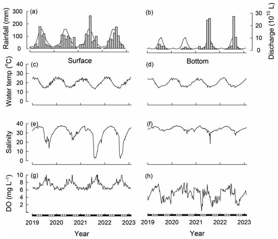
Figure 2.
Long-term average (line) and total monthly (bars) (a) rainfall (recorded at Perth Airport) [30] and (b) freshwater discharge into the Swan River (recorded at Walyunga) between 2019 and 2023 [41]. Weekly surface (0.5 m depth) and bottom (6.0 m depth) values for (c,d) water temperatures (e,f) salinities and (g,h) dissolved oxygen (DO) concentrations in the Swan-Canning Estuary basin (recorded at Heathcote) [41]. Black and white bars on x-axis refer to seasons.
The total annual streamflow into the Swan River ranged from 4.0 × 10¹⁰ L in 2020 to 60.6 × 10¹⁰ L in 2021 (long-term average = 28.5 × 10¹⁰ L). As with rainfall, the monthly average streamflow was highly seasonal, with 92% occurring between May and October (Figure 2b). Monthly streamflow was well below average in each month of the first two years of the study, but was above average in most months of 2021, including March, which produced 2.3 × 10¹⁰ L (average 0.2 × 10¹⁰ L), and June and July, which combined produced 48.3 × 10¹⁰ L (average combined 17.5 × 10¹⁰ L). While monthly streamflow values in 2022 were below average until July, August produced 26.5 × 10¹⁰ L, the most of any month over the study period and well above average for that month (9.5 × 10¹⁰ L; Figure 2b).
Water temperatures followed seasonal trends being warmer during the austral summer (December to February) and cooler during winter (June to August; Figure 2c). The surface water temperature over the study ranged from 13.1 °C during July 2021 to 26.6 °C during January 2022. Bottom water temperatures at the time of construction of the bouchot-style reefs was ~21 °C and declined to 14.7 °C in June 2019. Bottom water temperatures then increased progressively, attaining a maximum of 24.9 °C in December 2019 and typically remained >24° C until March 2020 and thus until the end of the monthly sampling regime. Bottom water temperatures during the winter of 2020 ranged between 14.9 and 16.9 °C before increasing to 25.2 °C in January 2021. They followed similar seasonal trends throughout 2021 and 2022, attaining their minimum of 14.8 °C during August 2021 and maximum of 25.6 °C during February 2022 (Figure 2d).
Salinities in surface waters were close to full strength seawater during the summer (36.0) but reached 38.2 in March 2020 and became diluted during winter/early spring, particularly in 2021 and 2022, when they attained minimum values of ~2.7 (Figure 2e). Bottom water salinity at the time of reef deployment (April 2019) was ~37 before dropping to 31.6 in September 2019. At the end of February 2020, bottom salinities were 36.7 and attained their maximum of 38.2 in the following month. Maximum bottom salinities in 2021 were 37.8 during March, and those in 2022 were 37.5 during April and minimum values were attained during August of each year, ranging from 18.3 in 2021 to 29.1 in 2020 (Figure 2f).
Dissolved oxygen concentrations in surface water ranged from ~5.8 to 11.7 mg L−1 and were thus well saturated throughout the study period (Figure 2g). In bottom waters, dissolved oxygen concentrations remained >2.0 mg L−1 throughout most of the study but were below that value on several occasions during 2021, including the majority of March and intermittently during August/September and then again during late September/early October 2022 (Figure 2h).
3.2. Mussel Performance
At the time of seeding in April 2019, shell lengths of M. galloprovincialis were 40–70 mm and produced a modal length of 55–60 mm (Figure 3). The modal length at each of the three reefs increased to 60–65 mm in June. While, by November, maximum lengths at Reef 1 were all <80 mm, several individuals at Reefs 2 and 3 had exceeded 85 mm.
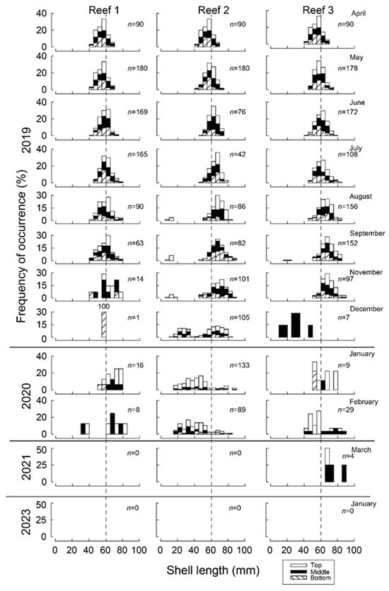
Figure 3.
Monthly shell length–frequency histograms (%) of 5 mm-length classes of translocated Mytilus galloprovincialis (and recruits) attached to the bottom, middle and top sections of wooden stakes used to create three bouchot-style reefs in the Swan-Canning Estuary. n = number of mussels sampled from three stakes from each reef in each month. Dashed vertical lines show shell length of 60 mm for reference.
Recruitment of a new cohort of mussels occurred at each reef site and was first detected in August at Reef 2, at which time they produced a modal length class of 10–15 mm. While the modal length of the new (2019) year class remained at 10–15 mm through to November (2019), it progressed to 20–30 mm in December and to 45–50 mm in January (2020). The number of new recruits were greatest at Reef 2, with 251 individuals collected between August and February, whereas only 2 and 28 were recorded at Reef 1 and Reef 3. Although there was a total of 89 individuals collected in February at Reef 2, this number declined to 0 by March 2021 and only 4 mussels were observed in all samples. No mussels were recorded in January 2023. While 72% of the 218 newly recruited mussels were sampled from the top section of the stake, only 6% were recorded on the bottom section of the stake (Figure 3).
Between May 2019 and February 2020, the mean lengths of M. galloprovincialis differed significantly between months, reef site and stake section (all p < 0.001) and significant interactions existed among the three factors (p = 0.038). The mean length at seeding in April was 51.9 mm (Figure 4). At the beginning of spring (September), the mean lengths attained ranged from 57.3 mm at Reef 1 to 67.5 mm at Reef 3. The mean length in each month was typically the lowest for the bottom section of the stake and greatest for the top section. For example, in September, the mean shell length at Reef 1 was 7.0 mm less on the bottom than the top stake section (Figure 4a).
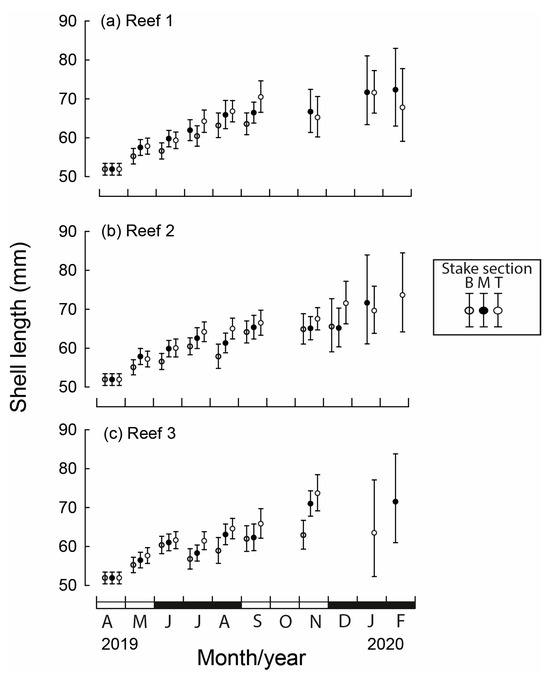
Figure 4.
Mean monthly (and 95% CI) shell lengths of translocated Mytilus galloprovincialis for each stake section (B = bottom, M = middle, T = top) at the three constructed bouchot-style reefs (a–c) in the Swan-Canning Estuary between April 2019 and February 2020. Black and white bars on x-axis refer to seasons.
Mass (standardised for shell length of 61 mm) differed statistically between months, reef site and stake section, as did the interaction between these three factors (all p < 0.001). At the time of translocation of M. galloprovincialis, the average mean dry tissue mass was 1.01 g (Figure 5). Declines in mass were most pronounced at Reef 1 with the mass after one month ranging from 0.65 g on the bottom section of the stake to 0.82 g on the top section and reached their lowest values during July to September (0.34–0.39 g; Figure 5a). At Reef 2, the mean mass initially increased on the top section of the stake (1.05 g), which was 0.25 g greater than the bottom section. While mass at Reef 2 attained their lowest value in July of 0.41–0.46 g, mass increased markedly in subsequent months, particularly for the top stake section, which reached 0.89 g in November (Figure 5b). Reef 3 followed similar monthly trends with the bottom stake section, always producing the lowest mean mass (Figure 5c).
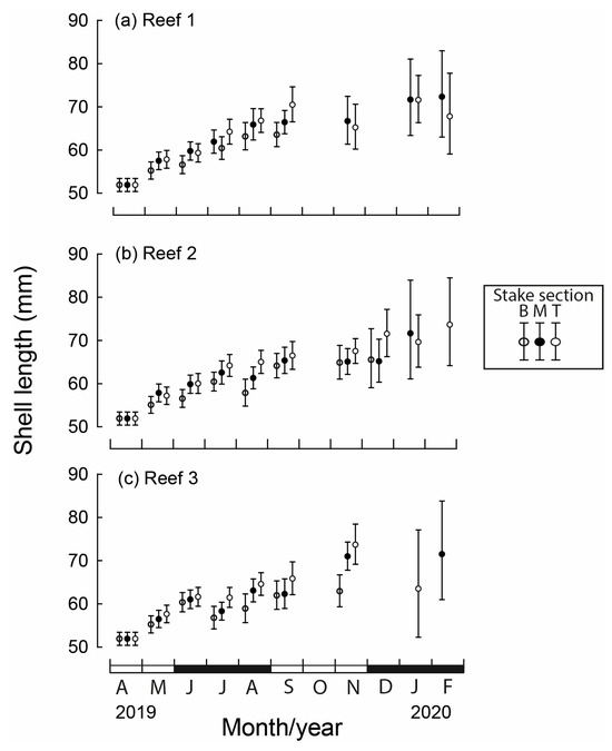
Figure 5.
Mean monthly (and 95% CI) mussel dry mass of translocated M. galloprovincialis (standardised for mean shell length of 61 mm) for each stake section (B = bottom, M = middle, T = top) at three bouchot-style reefs (a–c) in the Swan-Canning Estuary between April 2019 and February 2020. Black and white bars on x-axis refer to seasons.
Of the original 136 M. galloprovincialis seeded on each stake at the commencement of the study (April 2019), on average, between 83 and 91 survived for one month, representing a decline in numbers of 33–39% (Figure 6). While between May and September numbers declined by a further 68 to 75% at Reef 1 and Reef 2, numbers at Reef 3 declined by only 29%. By November, the average number of individuals per stake had declined to five at Reef 1, 26 at Reef 2 and 32 at Reef 3. High mortality continued at Reef 3 in the ensuing month, leaving <3 mussels per stake for the remainder of the study, which was similar to the number of mussels alive on each stake at Reefs 1 and 2. The overall numbers (May to February) were greatest at Reef 3 (1101 ind.) and least at Reef 1 (915 ind.), while Reef 2 contained 1007 individuals and the total numbers of individuals throughout the study were the greatest on stake top sections (1074 ind.) and lowest on bottom sections (904 ind.), while the middle section of the stake yielded 1045 individuals (Figure 6).
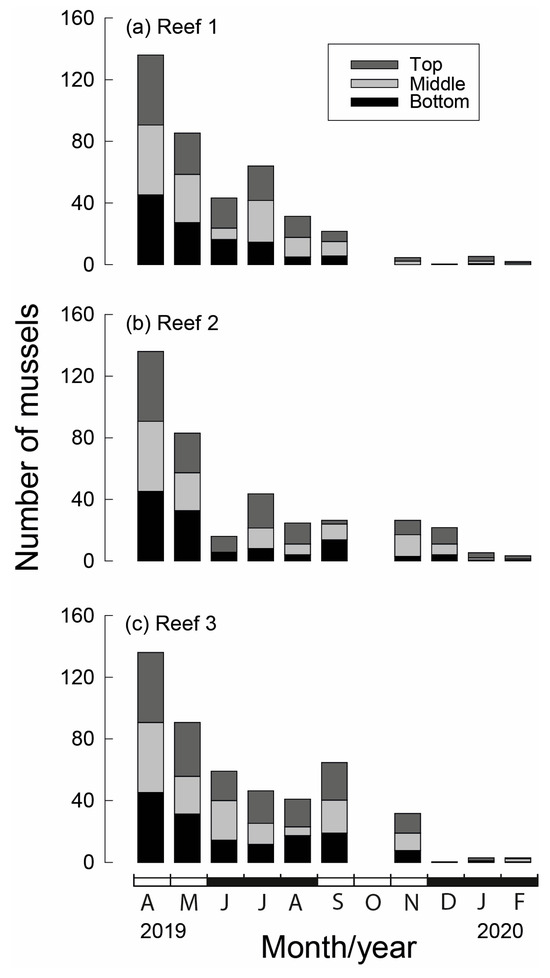
Figure 6.
Average number of translocated Mytilus galloprovincialis (ind. 300 mm−1) on each stake section (bottom, middle and top) at each of the three bouchot-style reefs (a–c) in the Swan-Canning Estuary in each month between April 2019, when they were seeded, and February 2020. Black and white bars on x-axis refer to seasons.
3.3. Fish Communities
A total MaxN of 6946 individuals, representing 31 fish species from 23 families, and one crustacean species (P. armatus) were recorded on RUVs at the bouchot-style reefs and control sites (Table 1). Before deployment of the reefs, 10 species were recorded from the 32 samples with a mean total MaxN of 12. After the deployment of the reefs, a larger number of species and mean total MaxN were recorded on the reefs (31 and 65.1, respectively) compared to the control site (17 and 51.1, respectively) from the 56 samples (Table 1). Only two species found on the control site were not detected on the reefs, albeit none were particularly abundant. The most notable difference in fish fauna between the two habitats after reef deployment was the much greater abundance of the apogonid Ostorhinchus rueppellii at the reefs than control sites (Table 1).

Table 1.
Mean MaxN (MN), standard deviation (SD), percentage contribution to MaxN (%C) and frequency of occurrence (%F) for each fish species recorded on RUVs at all sites before bouchot-style reef deployment (Pre; October-December 2018 and February 2019) and the control and reef sites after the deployment of the reefs (April 2019–June 2020) in the Swan-Canning Estuary. The estuarine usage guild (EUG), habitat guild (HG) and feeding guild (FG) and overall abundance (#) of each species are provided (Table A1). Semi-anadromous (SA), estuarine & freshwater (E&F), solely estuarine (E), estuarine & marine (E&F), marine estuarine-opportunists (MEO) and marine straggler (MS); pelagic (P), small pelagic (SP), benthopelagic (BP), demersal (D) and small benthic (SB); piscivore (PV), zooplanktivore (ZP), zoobenthivore (ZB), omnivore (OV), detritivore (DV) and opportunistic (OP). Taxon ranked by overall abundance. * denotes a crustacean species.
No significant differences were detected between the number of species or total MaxN among Habitat, Time or their interaction before deployment of the reefs (Table A2; Figure A1a–d). Faunal composition was shown not to differ significantly with Habitat, either as a main effect or in the Time × Habitat interaction term, although a difference over time was detected (Table A2). Pairwise PERMANOVA showed this was due to the fauna in October 2018 being distinct from those in all other time periods as well as that in November 2018 being different from February 2019. This is illustrated on the mMDS plots, where the 95% region estimates overlap substantially for Habitat; the points for October 2018 are predominantly discrete from other months, but February 2019 overlays December 2019 and the latter time with that of November 2018 (Figure 7). Temporal changes were driven by the fish community in October 2018 being depauperate and heavily dominated by Favonigobius punctatus and O. rueppellii, with other species such as the southern eagle ray Myliobatis tenuicaudatus recorded in all other months and P. armatus in November 2018, Helotes octolineatus in December 2018 and Atherinidae spp. and Sillago burrus in February 2019 (Figure A2).
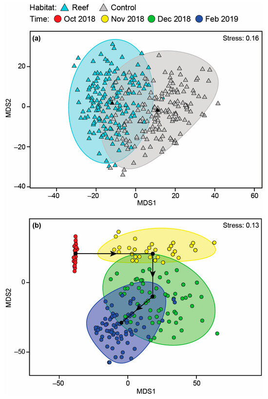
Figure 7.
Two-dimensional mMDS ordination plot constructed from bootstrap averages for (a) Habitat and (b) Time, calculated from a Bray–Curtis resemblance matrix of the MaxN of each fish species in each replicate sample collected before the bouchot-style reefs were deployed in the Swan-Canning Estuary. Group averages (larger symbols) and approximate 95% region estimates fitted to the bootstrap averages are provided.
Of the species recorded after reef deployment, 53 and 63% found on the control and reef sites, respectively, belonged to the marine category, i.e., marine estuarine-opportunists and marine stragglers (Table 2a). The reefs harbored two more species from the former guild and eight from the latter, while the numbers of estuarine species, i.e., solely estuarine, and estuarine & marine, were similar between both habitats. When based on the number of individuals, there was a ~60% increase in the number of marine estuarine-opportunists and a 72% increase in the number of marine stragglers at reef sites. There was also a 75% increase in the number of individuals of estuarine & marine species at reef than control sites despite both habitats containing four species. Based on feeding mode guilds, most species recorded in both habitats were zoobenthivores; however, far more species representing this guild were recorded on the reefs (16) than the control sites (10; Table 2b). Similarly, more omnivorous species were found on reefs (7) than control (2) sites. Combined, fish in these two guilds accounted for 94.6% of the total number of individuals at reefs and 76.8% at control sites and thus dominated the fish faunal community. Most of the species recorded belonged to the benthopelagic, demersal and small benthic habitat guilds, and constituted 29 of the 31 species (94%) at the reefs and 15 of the 17 (88%) at the control sites (Table 2c). Far more demersal species were present on the reefs (14 vs. 4), as were individuals of benthopelagic species (2748 vs. 1136). Although the small pelagic guild was represented by only two species at the control site, the schooling nature of these fish resulted in their individuals comprising 58% of all fish recorded (Table 2c).
Table 2.
Number of fish species (Sp) and individuals (N) of each of the (a) estuarine usage, (b) feeding and (c) habitat guilds, together with their percentage contribution (%), in RUV samples collected from the bouchot-style reefs and control sites in the Swan-Canning Estuary between April 2019 and June 2020.
Reef habitats harbored a significantly greater mean number of species (3.8) than control sites (3; Table A2b; Figure A1e). Values also changed over time, undergoing a sinusoidal trend, declining from ~4 in April 2019 to a minimum of 0.5 in June 2019, after which values increased essentially sequentially to ~6 between January and April 2020 before declining to ~2 in May and June of that year (Figure A1f). The total MaxN only differed significantly with Time (Table A2b), with values between January and April 2020 (~110 to 175) being larger than those in most other months and particularly between May and July 2019 (<15) and June 2020 (9; Figure A1g).
Fish faunal composition was found to differ significantly with Habitat and Time (Table A2c). On the associated mMDS plot, the 95% region estimates for the habitats were discrete, with the points for the reefs lying on the left of the plot clearly separated from those of the control sites (Figure 8b). The changes in faunal composition can be attributed to the wider range of species found at the reef sites including the aracanid Anoplocapros amydaloides (Figure 8a and Figure A3a), the syngnathid Hippocampus angustus and a range of leatherjackets, i.e., Monacanthus chinensis, Acanthaluteres vittiger, Eubalichthys mosaicus and Monacanthidae spp. Although O. rueppellii, H. octolineatus and the gobiid Arenigobius bifrenatus were found in both habitats, their abundances were all greater on the reef sites. It should be noted, however, that several species such as M. tenuicaudatus, Atherinidae spp. and the engraulid Engraulis australis were more abundant at control sites (Figure 8a and Figure A3a).
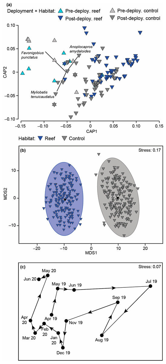
Figure 8.
(a) Canonical analysis of principal coordinate plot illustrating differences in the fish composition on the bouchot-style reefs and control sites before and after reef deployment. (b) Two-dimensional mMDS ordination plot constructed from bootstrap averages for Habitat, calculated from a Bray–Curtis resemblance matrix of the MaxN of each fish species in each replicate sample collected after the bouchot-style reefs were deployed in the Swan-Canning Estuary. Group averages (larger symbols) and approximate 95% region estimates fitted to the bootstrap averages are provided. (c) Centroid nMDS ordination plot derived from a distance among centroid matrix of the MaxN of each fish species for each sampling occasion (reefs and control combined). Arrows denote direction of cycling.
Post hoc analysis of the differences over time are provided in Table A3. When the fish community data were visualised on a centroid nMDS plot, the order of points formed a spiral (Figure 8c). There was a clockwise serial progression in samples between April 2019 to April 2020 before heading upwards and then to the left in May and June 2020. A core group of three species, i.e., O. rueppellii, A. bifrenatus and Torquigener pleurogramma, were found in all months and usually in relatively large abundances (Figure A3b). These species comprised the majority of the depauperate fauna observed between May and September 2019. In November and December 2019, additional species were recorded such as M. tenuicaudatus, F. punctatus, A. amydaloides, P. armatus and H. octolineatus. The last two species persisted for the next four months (January to April 2020) together with Pomatomus saltatrix, Acanthopagrus butcheri, Sillago burrus and Gerres subfasciatus.
3.4. Invertebrate Communities
Of the 18 species recorded (including M. galloprovincialis), 12 were native, and the remaining 6 were NIS (Table 3). The Acorn Barnacle Amphibalanus variegatus was the most numerous, comprising 36% of the individuals and occurring in ~80% of samples. The non-indigenous tube building polychaete Ficopomatus enigmatus was the next most abundant species, despite being recorded in only 5% of samples. The other abundant and consistently recorded species was the European sea squirt Ascidiella aspersa, a NIS (Table 3). The number of species differed significantly over time (Table A4a), increasing sequentially from 8 in May to 14 in December (2019) before declining to 4 in March 2021 (Figure 9a). Likewise, total abundance differed significantly with Time. Abundances declined sequentially between May and September 2019 before increasing in December of that year (Figure 9b). Very few individuals were recorded in March 2021 and were highest in January 2022. In the case of both variables, there was a significant Time × Site interaction; however, they explained only a small proportion of the variance (Table A4a,b).
Table 3.
List of native and non-indigenous (NIS) invertebrate species collected on the top section of wooden stakes used to create three bouchot-style reefs in the Swan-Canning Estuary and their mean abundance (Abund), standard error (SE), percentage contribution (%C), occurrence (i.e., number of samples species was found in; Occ) and frequency of occurrence (%F). Data for Mytilus galloprovincialis in bold.
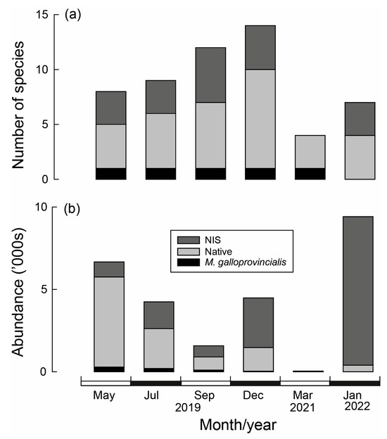
Figure 9.
(a) Number of NIS (non-indigenous species), native species and Mytilus galloprovincialis and (b) their abundance collected from wooden stakes used to create bouchot-style reefs in the Swan-Canning Estuary over time.
The composition of the invertebrate community differed with Time and Time × Site, but not Site (Table A4c), with pairwise testing demonstrating that a distinct fauna was recorded on each sampling occasion. This is shown on the mMDS plot where the bootstrapped averages for each occasion did not overlap and, in particular, that of March 2021 was distinct and widely separated from the other sampling occasions (Figure 10a). The relatively uninfluential Time × Site interaction was caused by the magnitude of the differences between sites increasing over time as the invertebrate composition of the reefs diverged (Figure 10c). CAP highlighted M. galloprovincialis, A. variegatus and A. aspersa as characterising the invertebrate fauna between May and September 2019, the native bivalve Fluviolanatus subtortus and NIS bivalve Asian Bag Mussel A. senhousia (December 2021 and January 2023) and sponges (March 2021; Figure 10d). Many of these trends were also supported by the shade plot, but this plot also highlighted the depauperate nature of the invertebrate fauna following the hypoxia in March 2021, and even though F. enigmatus ranked third in terms of abundance, it was only recorded at Reef 2 in January 2023 (Figure A4).
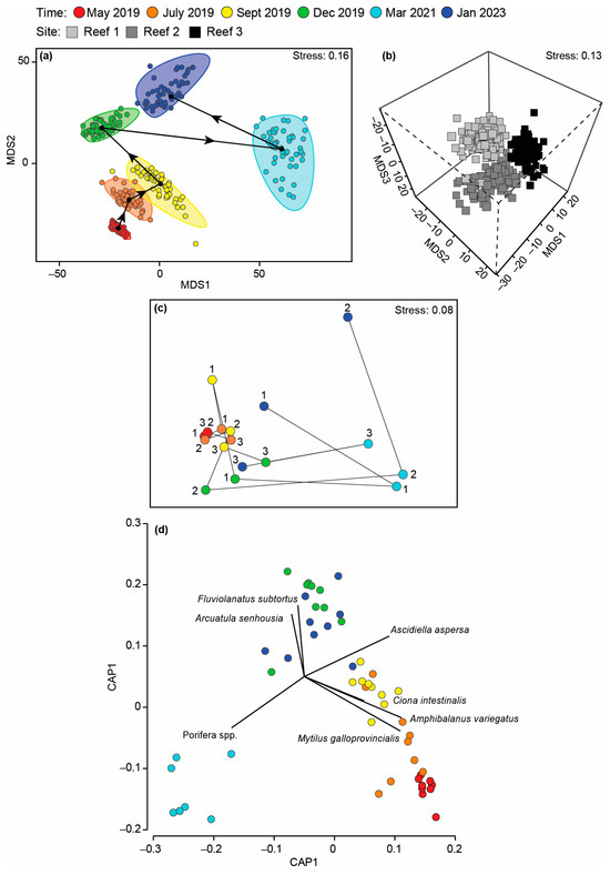
Figure 10.
mMDS ordination plot constructed from bootstrap averages for (a) Time and (b) Site, calculated from a Bray–Curtis resemblance matrix of the MaxN of each invertebrate species in each replicate sample collected after the bouchot-style reefs were deployed in the Swan-Canning Estuary. Group averages (larger symbols) and approximate 95% region estimates fitted to the bootstrap averages are provided. (c) Centroid nMDS ordination plot derived from a distance among centroid matrix of the abundance of each invertebrate species for each sampling occasion. Arrows denote direction of cycling. (d) Canonical analysis of principal coordinates plot illustrating differences in the invertebrate composition on the bouchot-style reefs over time.
4. Discussion
This study was the first to assess the efficacy of employing a bouchot-style approach as an option for shellfish reef restoration. This was assessed at three locations in the Swan-Canning Estuary through quantitative assessment of the biological characteristics (growth, body condition and survival) of translocated M. galloprovincialis, the presence of naturally recruited M. galloprovincialis and the suitability of the reef structure for fish and other macroinvertebrates. The study demonstrated that distance from sediment was an important factor when considering shellfish reef restoration approaches, with mussel survival, growth, body condition and recruitment greater on the top section of the stake. Furthermore, more fish species inhabited the bouchot-style reefs than unstructured habitats and the reefs were also colonised by a range of invertebrate species, including 11 native and 6 non-indigenous species; thus, this type of an approach has potential as a shellfish reef restoration option. However, due to bottom water hypoxia that can occur in wet years or following unseasonal rainfall, the study also found that the deeper waters of the estuary may not be conducive to sustaining populations of M. galloprovincialis over multiple years, the results of which can provide guidance for future shellfish restoration initiatives.
4.1. Overall Performance of Mytilus galloprovincialis
The performance (recruitment, growth, body condition and survival) of M. galloprovincialis differed among reef locations and particularly on stake section, i.e., distance from the substrate. Stake top sections, which were 700–1000 mm above the sediment, consistently outperformed those on the middle and bottom sections, which were 350–650 and 0–300 mm above the sediment, respectively. While the factors driving these marked differences among stake sections may be widely varying, the consistency in results implies that distance from substrate plays an important role, and this may be related to biotic and abiotic factors.
While the microtidal Swan-Canning Estuary contains weak tidal currents, its large width-to-depth ratio allows wind-generated waves to resuspend the fine sediments that are characteristic of estuary basins [7,13]. Although sediments can be displaced and distributed by turbulence throughout the water column, turbidity typically reaches its maximum near the seabed [54]. Thus, in close proximity to the seabed, particulate inorganic matter (PIM) concentrations are likely to exceed a threshold that mussels stop feeding, due to the metabolic cost of pseudofeces production and/or their sorting capacity becoming saturated [55,56,57,58]. It is thus relevant that in a recent study ~5 km upstream of Reef 1, where the performance of M. galloprovincialis was consistently poor, PIM in waters close to the seabed reached 305 mg L−1 (A. Cottingham unpublished data) and thus far greater than normal mussel feeding conditions (PIM < 10 mg L−1) [7,59,60]. Furthermore, these conditions are also more likely to be accompanied by lower dissolved oxygen concentrations [14].
4.2. Body Condition of Translocated Mytilus galloprovincialis
In most cases, the body condition of M. galloprovincialis decreased following translocation, particularly at Reef 1. This indicates that mussels are using energy reserves to survive, which is unsustainable over long durations [61,62]. This conclusion is consistent with recent M. galloprovincialis feeding behaviour experiments using water collected 0.5 m above the substrate in the basin of the Swan-Canning Estuary during summer, which yielded absorption efficiencies that were likely to equate to a net energy loss and thus progressive declining mass if conditions persist [7]. The low values for body condition during winter may have also be exacerbated by spawning [63,64] and these have been observed in other marine bivalves, such as the New Zealand green lipped mussel Perna canaliculus [65], and this may have further reduced glycogen reserves leading to increased vulnerability to stressful conditions [66]. The conclusion that spawning occurs in winter in the Swan-Canning Estuary was consistent with the presence of new recruits in samples in August.
4.3. Factors Influencing Reef Sustainability
Despite the lifespan of M. galloprovincialis typically ranging between two and four years, only 2% of translocated mussels survived until the end of the study, i.e., 10 months [67,68]. This rate was far lower than that recorded in a study in the Aegean Sea in which 77.5% of M. galloprovincialis in nets survived for a similar time [69]. While the low survival rate of translocated mussels is likely to be at least partly explained by sequential declines in body condition following translocation, only four mussels were recorded in all samples in March 2021, and those include those naturally recruited onto the reefs. The scarcity of M. galloprovincialis was accompanied by marked declines in other invertebrate species, which declined from 4495 individuals belonging to 14 species in December 2019 to 35 individuals belonging to 4 species in March 2021. Such consistency in declines in the number of species and individuals is important when considering potential drivers.
As the majority of species (both NIS and native) recorded on the bouchot-style reefs were temperate species, summer temperature may have exceeded critical thermal maximums for some of these. For example, the abundant native species A. variegatus has a similar geographic distribution to M. galloprovincialis and thus also likely has a similar temperature tolerance. It is thus relevant that the water temperature in the Swan-Canning Estuary was >24 °C for several months of the year, a temperature that has been associated with mass mortality of M. galloprovincialis [70]. While some of the abundant NIS species were introduced from cooler waters in Europe, e.g., A. aspersa, and thus also have a limited tolerance to elevated temperatures (26 °C) [71], A. senhousia has an upper thermal limit of 31 °C and is capable of surviving in salinities between 17 and 37 [72,73]. Thus, the temperatures and salinities in the current study remained well within the tolerance range for A. senhousia.
While mytilids generally have a better survival when exposed to low oxygen than most other invertebrate species, this tolerance has evolved from oversized lamellibranchiate gills that aid in filter feeding and the ability of mussels to survive during emersion over a tidal cycle [74,75]. For example, the blue mussel Mytilus edulis only showed a slight reduction in respiration rates when subjected to dissolved oxygen concentrations decreasing from 9 to 2 mg L−1 and demonstrated excellent survival (98%) when exposed to 2 mg L−1 for 16 days [75]. Mytilids also contain a robust mechanism to cope with these stressors, which involves isolating their living tissue through valve closure [7,76]. For example, the valves of M. galloprovincialis have been shown to close in response to declining salinities (~10) and hypoxic conditions [75,76]. During valve closure, however, oxygen concentrations in the mantle cavity can decline rapidly, resulting in a switch to anaerobic respiration [77]. Although this metabolic pathway still yields adequate amounts of ATP and glycogen stores [78,79], prolonged closure can result in substantial mortality [76]. For example, exposing M. galloprovincialis to a salinity of 5, thus inducing valve closure, resulted in 77% mortality after ~4 days [76]. It was thus relevant that dissolved oxygen concentrations during 2021 dropped below 2 mg L−1 for several weeks, conditions that are also considered lethal for most benthic invertebrates [80,81].
4.4. Faunal Composition
While the average number of species and total MaxN remained relatively constant throughout the four months prior to the reef deployment, a discernible temporal shift in faunal composition occurred following the first sampling occasion in October 2018, i.e., mid-spring, in which the fish community was depauperate. This is consistent with the well-established seasonal changes in the fish fauna of permanently-open temperate estuaries [82,83,84,85]. During summer and autumn months, when salinities and temperatures are elevated, the number of fish species with marine affinities are typically far greater than in winter, when salinities and temperatures decline [86,87]. Furthermore, it is relevant that the annual rainfall during that year (2018) of 744 mm would have produced water column stratification and reduced oxygen condition in bottom waters.
Following reef deployment, fish faunal composition differed significantly between the reef and control sites, with these differences largely attributed to the increased numbers of species utilising the reef habitat. Comparisons between structurally complex shellfish reef sites vs. unvegetated controls undertaken in other parts of the world have yielded similar results, which are explained by the provision of shelter and additional prey sources [10,88,89,90,91]. Almost all species found exclusively at reef sites, namely the boxfish A. amygdaloides, the seahorse H. angustus and several species of leatherjacket, e.g., Monacanthus chinensis, Acanthaluteres vittiger and Eubalichthys mosaicus, were marine species with a preference for complex structures [43,92,93,94]. While the number of benthopelagic species remained similar between reef and control habitat, there was a marked increase in abundance at the reef sites. This difference was largely driven by the apogonid, O. ruppelli, which formed large schools at the reef sites, capitalising on the increased structure and availability of its small crustacean prey [95].
The number of species, total MaxN and faunal composition of invertebrates all differed significantly between months, with successive increases in mean species richness reflecting colonisation of the reefs over time, and these were assisted by the provision of new surfaces as the numbers of M. galloprovincialis declined. Of the invertebrate species, those of barnacles and ascidians were the most abundant. The ascidian Ciona intestinalis, which is known to feed on bivalve larvae [96], was one of the most abundant species during winter (May–September 2019), which coincided with the spawning season of M. galloprovincialis. This ascidian then declined markedly in December, which may be attributed to the inability of this species to function at temperatures >21 °C [97]. Although this may not directly contribute to its mortality, it would have reduced its ability to compete, and this was evident as the presence of the colonial ascidian S. plicata increased during the warmer months. Although S. plicata was not abundant, its individuals were typically large. This species is also more tolerant to warmer waters and prefers higher salinities, which could explain its appearance in December and not in the cooler months when C. intestinalis was more abundant [98].
There was a marked shift in invertebrate composition in March 2021 following the prolonged period of hypoxia with species such as M. galloprovincialis, the barnacle A. variegatus and the ascidians C. intestinalis, A. aspersa and S. pilcata all disappearing and being replaced by sponges, which were only recorded in one of the three reefs and even then, in low quantities prior to hypoxia. Ascidians are considered fairly sensitive to low oxygen conditions, with several field studies demonstrating that C. intestinalis suffers mortality while oysters survived [96,99]. While M. galloprovincialis and a congener of A. variegatus have been shown to have considerable tolerance to hypoxia, they have a lower threshold than those of sponges [100], thus explaining why the latter taxa dominated at all reef sites in March 2021. However, their low abundance before March 2021 and in January 2023 suggests they are poor competitors, and their occurrence was likely linked to their ability to withstand prolonged hypoxia.
Although not contributing substantially to changes in faunal composition, it is important to note the impact of the non-native solitary ascidian A. aspersa and barnacle A. variegatus, which colonised the stakes rapidly upon their deployment. Both these species were recorded in high abundances throughout months and on all reefs. The rapid colonisation of the stakes particularly by A. aspersa may be attributed to its biology. This species can live for 18 months and adapt their reproductive biology from gonochoristic to a hermaphrodite to allow spawning to occur throughout the year [101]. Furthermore, A. aspersa is well suited to urbanised and highly eutrophic estuaries and deeper slow-moving waters [102], which are characteristic of the basin region of the Swan-Canning Estuary. These biological traits likely explain the lack of temporal change in the abundance of this NIS ascidian.
4.5. Contribution to Future Knowledge
Although M. galloprovincialis is found throughout the Swan-Canning Estuary, it is almost exclusively restricted to a ~1 m depth and is particularly abundant on hard substrates in the intertidal zone, the majority of which are man-made (e.g., jetties and pylons). The success of mytilids in the intertidal zone, compared to many other types of fauna (and flora), is largely attributed to the ability of mytilids to prevent desiccation by closing their valves during emersion. Thus, shellfish reef restoration using these types of species would be far better suited to nearshore shallow/intertidal zones.
In contrast, as supported by this study, subtidal hard structures can attract competition from a range of faunal groups, some of which were able to attain abundances far greater than M. galloprovincialis. While the majority of the first colonisers were native species, by December (after about six months), this trend reversed and NIS species dominated, which included A. aspersa, the tunicate Molgulidae sp. and A. senhousia. Thus, potential locations for shellfish reef restoration efforts should consider the types of species that may colonise these habitats and whether they are likely to outcompete the target species. Moreover, the timing of the deployment should, where possible, not coincide with the availability of larvae from NIS, which could settle on the newly available habitat. In the case of the Swan-Canning Estuary, and despite its environmental, cultural, and societal importance and its historic loss of shellfish reefs, the estuary contains 46 of the States’ 60 marine NIS [30], and deployment of hard structures in the vicinity of busy ports thus needs to be given consideration. While seeding densities, size at seeding and timing of reef constructions could potentially result in improved M. galloprovincialis performance, the ability of mussels (and other fauna) to be sustained over longer durations appears limited, particularly during wet years in bottom water, which can become hypoxic for long durations.
5. Conclusions
Bouchots have been wildly used as a technique for mussel farming, and this study assessed the potential of using this method as a restoration tool for M. galloprovincialis in the Swan-Canning Estuary. Once deployed, the bouchot-style reefs were colonised by a range of invertebrate species and supported a more diverse fish fauna than unstructured control sites. However, the survival of translocated mussels was very low (60% initially and 2% after 10 months), likely due to periods of high water temperature or hypoxia and competition with non-indigenous species. The fact that hypoxia typically only occurs at the bottom of the water column, that mussel survival was greatest in the top section of the stake and that self-sustaining populations of M. galloprovincialis occur naturally in shallower waters in this estuary suggests that this restoration method could be successful in the Swan-Canning Estuary if appropriate sites, e.g., in nearshore shallow and/or intertidal zones, where able to be chosen. There would also be value in assessing the potential to utilise bouchot-style reefs as a restoration option for estuaries and coasts in other parts of the world where hypoxia occurs less frequently.
Author Contributions
A.C. and J.R.T. played a major role in supervision, conceptualization, methodology, visualisation and funding acquisition. C.M. and A.B. undertook the formal analysis and investigation. C.M. undertook the original draft preparation. All authors contributed to the writing—review and editing. All authors have read and agreed to the published version of the manuscript.
Funding
This research was funded by Recfishwest through the Recreational Fishing Initiatives Fund, the Department of Primary Industries and Regional Development.
Institutional Review Board Statement
The animal study protocol was approved by the Ethics Committee of Murdoch University (O2996/17).
Informed Consent Statement
Not applicable.
Data Availability Statement
Data are available on request.
Acknowledgments
Gratitude is expressed to volunteers and Murdoch University Dive Club for assistance in deploying the structures.
Conflicts of Interest
The authors declare no conflict of interest.
Appendix A
Table A1.
Definitions of the categories and/or guilds in the (a) estuarine usage, (b) feeding mode and (c) habitat functional groups (see [44,45]) assigned to fish species in the current study.
Table A1.
Definitions of the categories and/or guilds in the (a) estuarine usage, (b) feeding mode and (c) habitat functional groups (see [44,45]) assigned to fish species in the current study.
| (a) Estuarine usage functional group | |
| Category and/or guild | Definition |
| Marine category | Species that spawn at sea. |
| Marine straggler | Typically enter estuaries sporadically and in low numbers and are most common in the lower reaches where salinities typically do not decline far below ~35. Belong to populations in marine waters and are often stenohaline. |
| Marine estuarine opportunist | Regularly enter estuaries in substantial numbers, particularly as juveniles, but use, to varying degrees, coastal marine waters as alternative nursery areas. |
| Estuarine category | Species with populations in which the individuals complete their life cycles within the estuary. |
| Solely estuarine | Species found only in estuaries. |
| Estuarine & marine | Species also represented by marine populations. |
| Estuarine & freshwater | Species also represented by freshwater populations. |
| Diadromous category | Fish species which migrate between the sea and fresh water. |
| Semi-anadromous | Spawning run from the sea extends only as far as the upper estuary rather than into fresh water. |
| (b) Feeding mode functional group | |
| Guild | Definition |
| Piscivore | Feeding predominantly on finfish but may include large nektonic invertebrates. |
| Zooplanktivore | Feeding predominantly on zooplankton (e.g., planktonic crustaceans, fish eggs/larvae). |
| Zoobenthivore | Feeding predominantly on invertebrates associated with the substratum, including zoobenthos and hyperbenthos. |
| Omnivore | Feeding predominantly on filamentous algae, macrophytes, periphyton, epifauna and infauna. |
| Detritivore | Feeding predominantly on benthic detritus, microphytobenthos and associated meiofauna. |
| Opportunist | Feeing on consume a wide variety of prey, the components of which change with availability. |
| (c) Habitat mode functional group | |
| Guild | Definition |
| Pelagic | Medium to large species that occupy the middle and surface parts of the water column. |
| Small pelagic | Small-bodied, usually schooling species, present in the middle and surface parts of the water column. |
| Benthopelagic | Species found throughout the water column. |
| Demersal | Species that live and feed on or close to the bottom of the water column. |
| Small benthic | Small-bodied species living on or in the substrate. |
Table A2.
Mean squares (MS) and percentage contribution of mean squares (%MS), pseudo-F ratios (pF) and significance level (p) derived from two-way PERMANOVA tests on the (a) number of species and (b) total MaxN and (c) fish faunal composition of bouchot-style reefs and control sites before (Pre) and after (Post) reef deployment. Significant results (p = < 0.05) are highlighted in bold, and those significant and with a %MS ≥ 25 are shaded grey.
| Pre-Deployment | Post-Deployment | |||||||||
|---|---|---|---|---|---|---|---|---|---|---|
| (a) No. of species | df | MS | %MS | pF | p | df | MS | %MS | pF | p |
| Time | 3 | 1.86 | 28.98 | 1.03 | 0.389 | 13 | 25.85 | 54.96 | 11.22 | 0.001 |
| Habitat | 1 | 2.67 | 41.48 | 1.47 | 0.229 | 1 | 15.64 | 33.25 | 6.79 | 0.011 |
| Time × Habitat | 3 | 0.09 | 1.32 | 0.05 | 0.987 | 13 | 3.24 | 6.88 | 1.40 | 0.178 |
| Residual | 17 | 1.81 | 28.21 | 86 | 2.30 | 4.90 | ||||
| (b) Total MaxN | ||||||||||
| Time | 3 | 1.31 | 35.04 | 1.88 | 0.181 | 13 | 5.06 | 57.68 | 6.10 | 0.001 |
| Habitat | 1 | 1.50 | 40.23 | 2.16 | 0.159 | 1 | 2.30 | 26.20 | 2.77 | 0.118 |
| Time × Habitat | 3 | 0.23 | 6.09 | 0.33 | 0.826 | 13 | 0.58 | 6.66 | 0.70 | 0.740 |
| Residual | 17 | 0.69 | 18.64 | 86 | 0.83 | 9.46 | ||||
| (c) Faunal composition | ||||||||||
| Time | 3 | 7702 | 49.54 | 2.34 | 0.013 | 13 | 8303 | 37.08 | 3.46 | 0.001 |
| Habitat | 1 | 3202 | 20.60 | 0.97 | 0.436 | 1 | 9026 | 40.32 | 3.76 | 0.001 |
| Time × Habitat | 3 | 1349 | 8.68 | 0.41 | 0.975 | 13 | 2661 | 11.88 | 1.11 | 0.242 |
| Residual | 17 | 3293 | 21.18 | 86 | 2399 | 10.71 | ||||

Figure A1.
Mean (±95% confidence limits) number of species and total Max among habitats and dates before and after the deployment of the bouchot-style reefs in the Swan-Canning Estuary.
Figure A1.
Mean (±95% confidence limits) number of species and total Max among habitats and dates before and after the deployment of the bouchot-style reefs in the Swan-Canning Estuary.


Figure A2.
Shade plot constructed using transformed MaxN of each fish species recorded at the sites where the bouchot-style reefs would be deployed and the control sites over time.
Figure A2.
Shade plot constructed using transformed MaxN of each fish species recorded at the sites where the bouchot-style reefs would be deployed and the control sites over time.

Table A3.
t-statistic and significance level (p) values derived from a pairwise PERMANOVA test on the composition of the fish fauna recorded on the bouchot-style reefs and control sites combined among sampling occasions. t-statistic values are shaded grey if the pairwise compassion was significant (p = ≤ 0.05).
| 2019 | 2020 | ||||||||||||
|---|---|---|---|---|---|---|---|---|---|---|---|---|---|
| Month | Apr | May | Jun | Jul | Aug | Sep | Nov | Dec | Jan | Feb | Mar | Apr | May |
| May | 1.217 | ||||||||||||
| Jun | 1.392 | 0.478 | |||||||||||
| Jul | 2.731 | 2.672 | 2.032 | ||||||||||
| Aug | 1.642 | 1.865 | 1.614 | 2.262 | |||||||||
| Sep | 1.612 | 1.638 | 1.226 | 0.980 | 1.242 | ||||||||
| Nov | 0.865 | 1.653 | 1.593 | 2.743 | 1.935 | 1.715 | |||||||
| Dec | 1.236 | 2.061 | 1.960 | 2.838 | 1.777 | 1.748 | 0.711 | ||||||
| Jan | 1.026 | 1.654 | 1.657 | 2.763 | 1.522 | 1.556 | 1.269 | 1.139 | |||||
| Feb | 1.118 | 1.536 | 1.594 | 2.817 | 1.896 | 1.646 | 1.459 | 1.476 | 0.902 | ||||
| Mar | 1.255 | 1.737 | 1.861 | 3.204 | 2.015 | 1.802 | 1.725 | 1.714 | 1.041 | 0.881 | |||
| Apr | 1.359 | 1.825 | 2.005 | 3.591 | 2.397 | 2.214 | 1.585 | 1.561 | 1.398 | 1.098 | 1.017 | ||
| May | 1.473 | 1.072 | 1.324 | 2.997 | 2.330 | 1.948 | 1.820 | 2.284 | 2.053 | 1.950 | 2.185 | 2.201 | |
| Jun | 1.608 | 0.978 | 1.346 | 3.511 | 2.503 | 2.249 | 2.032 | 2.594 | 2.266 | 1.992 | 2.268 | 2.335 | 0.693 |

Figure A3.
Shade plot constructed using transformed MaxN of each fish species recorded on (a) the bouchot-style reefs and control sites and (b) among both habitats over time.
Figure A3.
Shade plot constructed using transformed MaxN of each fish species recorded on (a) the bouchot-style reefs and control sites and (b) among both habitats over time.

Table A4.
Mean squares (MS) and percentage contribution of mean squares (%MS), pseudo-F ratios (pF) and significance level (p) derived from two-way PERMANOVA tests on the (a) number of species (b) number of individuals and (c) faunal composition of invertebrate species collected on the top section of wooden stakes used to create the bouchot-style reefs in the Swan-Canning Estuary. Significant results (p = <0.05) are highlighted in bold, and those significant and with a %MS ≥ 25 are shaded grey.
| (a) Number of species | df | MS | %MS | pF | p |
| Time | 5 | 33.56 | 81.67 | 27.05 | 0.001 |
| Site | 2 | 3.17 | 7.71 | 2.55 | 0.092 |
| Time × Site | 10 | 3.12 | 7.60 | 2.52 | 0.017 |
| Residual | 36 | 1.25 | 3.02 | ||
| (b) Number of individuals | |||||
| Time | 5 | 1.16 | 73.65 | 18.35 | 0.001 |
| Site | 2 | 0.17 | 10.52 | 2.62 | 0.073 |
| Time × Site | 10 | 0.19 | 11.82 | 2.94 | 0.011 |
| Residual | 36 | 0.06 | 4.02 | ||
| (c) Faunal composition | |||||
| Time | 5 | 33.56 | 81.67 | 27.05 | 0.001 |
| Site | 2 | 3.17 | 7.71 | 2.55 | 0.092 |
| Time × Site | 10 | 3.12 | 7.60 | 2.52 | 0.017 |
| Residual | 36 | 1.24 | 3.02 | ||

Figure A4.
Shade plot constructed using transformed abundances of each invertebrate species recorded on each of the three bouchot-style reefs over time.
Figure A4.
Shade plot constructed using transformed abundances of each invertebrate species recorded on each of the three bouchot-style reefs over time.

References
- Lunt, I.D.; Byrne, M.; Hellmann, J.J.; Mitchell, N.J.; Garnett, S.T.; Hayward, M.W.; Martin, T.G.; McDonald-Maddden, E.; Williams, S.E.; Zander, K.K. Using assisted colonisation to conserve biodiversity and restore ecosystem function under climate change. Biol. Conserv. 2013, 157, 172–177. [Google Scholar] [CrossRef]
- Coleman, M.A.; Wood, G.; Filbee-Dexter, K.; Minne, A.J.P.; Goold, H.D.; Vergés, A.; Marzinelli, E.M.; Steinberg, P.D.; Wernberg, T. Restore or redefine: Future trajectories for restoration. Front. Mar. Sci. 2020, 7, 237. [Google Scholar] [CrossRef]
- Jackson, J.B.C.; Kirby, M.X.; Berger, W.H.; Bjorndal, K.A.; Botsford, L.W.; Bourque, B.J.; Bradbury, R.H.; Cooke, R.G.; Erlandson, J.; Estes, J.A.; et al. Historical overfishing and the recent collapse of coastal ecosystems. Science 2001, 293, 629–638. [Google Scholar] [CrossRef] [PubMed]
- Beck, M.W.; Brumbaugh, R.D.; Airoldi, L.; Carranza, A.; Coen, L.D.; Crawford, C.; Defeo, O.; Edgar, G.J.; Hancock, B.; Kay, M.C.; et al. Oyster reefs at risk and recommendations for conservation, restoration, and management. Bioscience 2011, 61, 107–116. [Google Scholar] [CrossRef]
- Gillies, C.L.; McLeod, I.M.; Alleway, H.K.; Cook, P.; Crawford, C.; Creighton, C.; Diggles, B.; Ford, J.; Hamer, P.; Heller-Wagner, G.; et al. Australian shellfish ecosystems: Past distribution, current status and future direction. PLoS ONE 2018, 13, e0190914. [Google Scholar] [CrossRef] [PubMed]
- Lipcius, R.N.; Burke, R.P. Successful recruitment, survival and long-term persistence of eastern oyster and hooked mussel on a subtidal, artificial restoration reef system in Chesapeake Bay. PLoS ONE 2018, 13, e0204329. [Google Scholar] [CrossRef] [PubMed]
- Cottingham, A.; Bossie, A.; Valesini, F.; Tweedley, J.R.; Galimany, E. Quantifying the potential water filtration capacity of a man-made shellfish reef in a temperate hypereutrophic estuary. Diversity 2023, 15, 113. [Google Scholar] [CrossRef]
- McAfee, D.; McLeod, I.M.; Alleway, H.K.; Bishop, M.J.; Branigan, S.; Connell, S.D.; Copeland, C.; Crawford, C.M.; Diggles, B.K.; Fitzsimons, J.A.; et al. Turning a lost reef ecosystem into a national restoration program. Biol. Conserv. 2022, 36, e13958. [Google Scholar] [CrossRef]
- zu Ermgassen, P.S.E.; Grabowski, J.H.; Gair, J.R.; Powers, S.P. Quantifying fish and mobile invertebrate production from a threatened nursery habitat. J. Appl. Ecol. 2016, 53, 596–606. [Google Scholar] [CrossRef]
- Christianen, M.J.; Van der Heide, T.; Holthuijsen, S.J.; Van der Reijden, K.J.; Borst, A.C.; Olff, H. Biodiversity and food web indicators of community recovery in intertidal shellfish reefs. Biol. Conserv. 2017, 213, 317–324. [Google Scholar] [CrossRef]
- Pfirrmann, B.W.; Seiz, R.D. Ecosystem services of restored oyster reefs in a Chesapeake Bay tributary: Abundance and foraging of estuarine fishes. Mar. Ecol. Prog. Ser. 2019, 628, 155–169. [Google Scholar] [CrossRef]
- Fréchette, M.; Daigle, G. Reduced growth of Iceland scallops Chlamys islandica (O.F. Müller) cultured near the bottom: A modelling study of alternative hypotheses. J. Shellfish Res. 2002, 21, 87–91. [Google Scholar]
- Cho, H.J. Effects of prevailing winds on turbidity of a shallow estuary. Int. J. Environ. Res. Public Health 2007, 4, 185–192. [Google Scholar] [CrossRef] [PubMed]
- Lorke, A.; Macintyre, S. The benthic boundary layer (in Rivers, Lakes, and Reservoirs). In Encyclopaedia of Inland Waters; Likens, G.E., Ed.; Elsevier: Oxford, UK, 2009; Volume 1, pp. 505–514. [Google Scholar]
- Sarà, G. Variation of suspended and sedimentary organic matter with depth in shallow coastal waters. Wetlands 2009, 29, 1234–1242. [Google Scholar] [CrossRef]
- Navarro, E.; Iglesias, J.I.P.; Camacho, A.P.; Labarata, U. The effect of diets of phytoplankton and suspended bottom material on feeding and absorption of raft mussels (Mytilus galloprovincialis Lmk). J. Exp. Mar. Biol. Ecol. 1996, 198, 175–189. [Google Scholar] [CrossRef]
- Ellis, J.; Cummings, V.; Hewitt, J.; Thrush, S.; Norkko, A. Determining effects of suspended sediment on condition of a suspension feeding bivalve (Atrina zelandica): Results of a survey, a laboratory experiment and a field transplant experiment. J. Exp. Mar. Biol. Ecol. 2002, 267, 147–174. [Google Scholar] [CrossRef]
- Suchanek, T.H. Extreme biodiversity in the marine environment mussel bed communities of Mytilus californianus. Northwest Environ. J. 1992, 8, 150–152. [Google Scholar]
- Smith, J.R.; Fong, P.; Ambrose, R.F. Dramatic declines in mussel bed community diversity: Response to climate change? Ecology 2006, 87, 1153–1161. [Google Scholar] [CrossRef]
- Lindberg, C.; Griffiths, C.L.; Anderson, R.J. Colonisation of South African kelp-bed canopies by the alien mussel Mytilus galloprovincialis: Extent and implications of a novel bioinvasion. Afr. J. Mar. Sci. 2020, 42, 167–176. [Google Scholar] [CrossRef]
- Brearley, A. Ernest Hodgkin’s Swanland. Estuaries and Coastal Lagoons of South-Western Australia; University of Western Australia Press: Perth, Australia, 2005. [Google Scholar]
- Christensen, J.; Martin, D.J.; Bossie, A.; Valesini, F. Middle Holocene oyster shells and the shifting role of history in ecological restoration: How a dynamic past informs shellfish ecosystem reconstruction at an Australian urban estuary. Glob. Environ. 2023, 16, 414–448. [Google Scholar] [CrossRef]
- Hallett, C.S.; Hobday, A.J.; Tweedley, J.R.; Thompson, P.A.; McMahon, K.; Valesini, F.J. Observed and predicted impacts of climate change on the estuaries of south-western Australia, a Mediterranean climate region. Reg. Environ. Chang. 2018, 18, 1357–1373. [Google Scholar] [CrossRef]
- Berthot, A.; Pattiaratchi, C.B.; Feng, M.; Meyers, G.; Li, Y. Understanding the natural variability of currents along the Western Australian coastline: Inter-annual variability of the Leeuwin Current. In Strategic Research Fund for the Marine Environment Final Report 1; University of Western Australia: Perth, Australia, 2007; pp. 117–183. [Google Scholar]
- Petrone, K.C.; Hughes, J.D.; Van Niel, T.G.; Silberstein, R.P. Streamflow decline in southwestern Australia, 1950–2008. Geophys. Res. Lett. 2010, 37, 11. [Google Scholar] [CrossRef]
- Silberstein, R.P.; Aryal, S.K.; Durrant, J.; Pearcey, M.; Braccia, M.; Charles, S.P.; McFarlane, D.J. Climate change and runoff in south-western Australia. J. Hydrol. 2012, 475, 441–455. [Google Scholar] [CrossRef]
- Smith, I.; Power, S. Past and future changes to inflows into Perth (Western Australia) dams. J. Hydrol. Reg. Stud. 2014, 2, 84–96. [Google Scholar] [CrossRef]
- Cottingham, A.; Hesp, S.A.; Hall, N.G.; Hipsey, M.R.; Potter, I.C. Marked deleterious changes in the condition, growth and maturity schedules of Acanthopagrus butcheri (Sparidae) in an estuary reflect environmental degradation. Estuar. Coast. Shelf Sci. 2014, 149, 109–119. [Google Scholar] [CrossRef]
- Cloern, J.E.; Foster, S.Q.; Kleckner, A.E. Phytoplankton primary production in the world’s estuarine-coastal ecosystems. Biogeosciences 2014, 11, 2477–2501. [Google Scholar] [CrossRef]
- Huisman, J.M.; Jones, D.S.; Wells, F.E.; Burton, T. Introduced marine biota in Western Australian waters. Rec. West. Aust. Mus. 2008, 25, 1–44. [Google Scholar] [CrossRef][Green Version]
- Cottingham, A.; Bossie, A.; Valesini, F.; Maus, C.; Tweedley, J.R. Habitat compression of an estuarine mytilid following half a century of streamflow decline. Estuar. Coast. Shelf Sci. 2023, 282, 108253. [Google Scholar] [CrossRef]
- Australian Government Bureau of Meteorology. Climate Change and Variability. 2023. Available online: http://www.bom.gov.au/jsp/ncc/cdio/weatherData/av?p_nccObsCode=139&p_display_type=dataFile&p_startYear=&p_c=&p_stn_num=009021 (accessed on 2 June 2023).
- Valesini, F.; Cottingham, A.; Hallett, C.S.; Clarke, K.R. Interdecadal changes in the community, population and individual levels of the fish fauna of an extensively modified estuary. J. Fish Biol. 2017, 90, 1734–1767. [Google Scholar] [CrossRef]
- Tweedley, J.R.; Hallett, C.S.; Warwick, R.M.; Clarke, K.R.; Potter, I.C. The hypoxia that developed in a microtidal estuary following an extreme storm produced dramatic changes in the benthos. Mar. Freshw. Res. 2016, 67, 327–341. [Google Scholar] [CrossRef]
- Poh, B.; Tweedley, J.R.; Chaplin, J.A.; Trayler, K.M.; Crisp, J.A.; Loneragan, N.R. Influence of physico-chemical and biotic factors on the distribution of a penaeid in a temperate estuary. Estuar. Coast. Shelf Sci. 2019, 218, 70–85. [Google Scholar] [CrossRef]
- Dias, P.J.; Fotedar, S.; Snow, M. Characterisation of mussel (Mytilus sp.) populations in Western Australia and evaluation of potential genetic impacts of mussel spat translocation from interstate. Mar. Freshw. Res. 2014, 65, 486–496. [Google Scholar] [CrossRef]
- FAO. The State of World Fisheries and Aquaculture 2022. Towards Blue Transformation; FAO: Rome, Italy, 2022. [Google Scholar]
- Gosling, E. Bivalve Molluscs: Biology, Ecology and Culture; Blackwell Publishing Limited: Hoboken, NJ, USA, 2002. [Google Scholar]
- Tweedley, J.R.; Loneragan, N.R.; Crisp, J.A.; Poh BBroadley, A.D.; Bennett, A.L.; Hodson, K.P.; Trayler, K.M.; Jenkins, G.I.; Chaplin, J.A. Stock Enhancement of the Western School Prawn (Metapenaeus dalli) in the Swan-Canning Estuary: Evaluating Recruitment limitation, Environment and Release Strategies; Report for the Fisheries Research and Development Corporation; Murdoch University: Perth, Australia, 2017. [Google Scholar]
- Tweedley, J.R.; Warwick, R.M.; Hallett, C.S.; Potter, I.C. Fish-based indicators of estuarine condition that do not require reference data. Estuar. Coast. Shelf Sci. 2017, 191, 209–220. [Google Scholar] [CrossRef]
- Department of Water and Environmental Regulation. 2023. Water Information Reporting. Available online: http://wir.water.wa.gov.au/Pages/Water-Information-Reporting.aspx (accessed on 11 May 2023).
- Obregón, C.; Christensen, J.; Zeller, D.; Hughes, M.; Tweedley, J.R.; Gaynor ALoneragan, N.R. Local fisher knowledge reveals changes in size of blue swimmer crabs in small-scale fisheries. Mar. Policy 2022, 143, 105144. [Google Scholar] [CrossRef]
- Florisson, J.H.; Tweedley, J.R.; Walker, T.H.E.; Chaplin, J.A. Reef vision: A citizen science program for monitoring the fish faunas of artificial reefs. Fish. Res. 2018, 206, 296–308. [Google Scholar] [CrossRef]
- Potter, I.C.; Tweedley, J.R.; Elliott, M.; Whitfield, A.K. The ways in which fish use estuaries: A refinement and expansion of the guild approach. Fish Fish. 2015, 16, 230–239. [Google Scholar] [CrossRef]
- Whitfield, A.K.; Able, K.W.; Blaber, S.J.M.; Elliott, M.; Franco, A.; Harrison, T.D.; Potter, I.C.; Tweedley, J.R. Fish assemblages and functional groups. In Fish and Fisheries in Estuaries—A Global Perspective; Whitfield, A.K., Able, K.W., Blaber, S.J.M., Elliott, M., Eds.; Wiley Blackwell: Hoboken, NJ, USA, 2022; pp. 16–59. [Google Scholar]
- Atkinson, C.L.; Parr, T.B.; van Ee, B.C.; Knapp, D.D.; Winebarger, M.; Madoni, K.J.; Haag, W.R. Length-mass equations for freshwater unionid mussel assemblages: Implications for estimating ecosystem function. Freshw. Sci. 2020, 39, 377–390. [Google Scholar] [CrossRef]
- Alunno-Bruscia, M.; Bourget, E.; Fréchette, M. Shell allometry and length-mass-density relationship for Mytilus edulis in an experimental food-regulated situation. Mar. Ecol. Prog. Ser. 2001, 219, 177–188. [Google Scholar] [CrossRef]
- Anderson, M.; Gorley, R.N.; Clarke, K.R. PERMANOVA + for PRIMER. Guide to Software and Statistical Methods; Primer-E: Plymouth, UK, 2008. [Google Scholar]
- Clarke, K.R.; Chapman, M.G.; Somerfield, P.J.; Needham, H.R. Dispersion-based weighting of species counts in assemblage analyses. Mar. Ecol. Prog. Ser. 2006, 320, 11–27. [Google Scholar] [CrossRef]
- Clarke, K.R.; Gorley, R.N.; Somerfield, P.J.; Warwick, R.M. Change in Marine Communities: An Approach to Statistical Analysis and Interpretation; Primer-E Ltd.: Plymouth, UK, 2014. [Google Scholar]
- Clarke, K.R.; Gorley, R.N. Primer: User Manual/Tutorial; Primer-E Ltd.: Plymouth, UK, 2015; p. 296. [Google Scholar]
- Lek, E.; Fairclough, D.V.; Platell, M.E.; Clarke, K.R.; Tweedley, J.R.; Potter, I.C. To what extent are the dietary compositions of three abundant, co-occurring labrid species different and related to latitude, habitat, body size and season? J. Fish Biol. 2011, 78, 1913–1943. [Google Scholar] [CrossRef]
- Clarke, K.R.; Tweedley, J.R.; Valesini, F.J. Simple shade plots aid better long-term choices of data pre-treatment in multivariate assemblage studies. J. Mar. Biol. Assoc. U. K. 2014, 94, 1–16. [Google Scholar] [CrossRef]
- Zikhali, V.; Tirok, K.; Stretch, D. Sediment resuspension in a shallow lake with muddy substrates: St Lucia, South Africa. Cont. Shelf Res. 2015, 108, 112–120. [Google Scholar] [CrossRef]
- Bayne, B.L.; Hawkins, A.J.S.; Navarro, E.; Iglesias, J.I.P. Effects of seston concentration on feeding, digestion and growth in the mussel Mytilus edulis. Mar. Ecol. Prog. Ser. 1989, 55, 47–54. [Google Scholar] [CrossRef]
- Madon, S.P.; Schneider, D.W.; Stoeckel, J.A.; Sparks, R.E. Effects of inorganic sediment and food concentrations on energetic processes of the zebra mussel, Dreissena polymorpha: Implications for growth in turbid rivers. Can. J. Fish. Aquat. Sci. 1998, 55, 401–413. [Google Scholar] [CrossRef]
- Maire, O.; Amouroux, J.M.; Duchêne, J.C.; Grémare, A. Relationship between filtration activity and food availability in the Mediterranean mussel Mytilus galloprovincialis. Mar. Biol. 2007, 152, 1293–1307. [Google Scholar] [CrossRef]
- Galimany, E.; Ramón, M.; Ibarrola, I. Feeding behavior of the mussel Mytilus galloprovincialis (L.) in a Mediterranean estuary: A field study. Aquaculture 2011, 314, 236–243. [Google Scholar] [CrossRef]
- Gardner, J.P.A. Effects of seston variability on the clearance rate and absorption efficiency of the mussel Aulacomya maoriana, Mytilus galloprovincialis and Perna canaliculus from New Zealand. J. Exp. Mar. Biol. Ecol. 2002, 268, 83–101. [Google Scholar] [CrossRef]
- Galimany, E.; Lunt, J.; Domingos, A.; Paul, V.J. Feeding behavior of the native mussel Ischadium recurvum and the invasive mussels Mytella charruana and Perna viridis in FL, USA, across a salinity gradient. Estuaries Coasts 2018, 41, 2378–2388. [Google Scholar] [CrossRef]
- Anestis, A.; Pörtner, H.O.; Karagiannis, D.; Angelidis, P.; Staikou, A.; Michaelidis, B. Response of Mytilus galloprovincialis (L.) to increasing seawater temperature and to marteliosis: Metabolic and physiological parameters. Comp. Biochem. Physiol. Part A Mol. Integr. Physiol. 2010, 156, 57–66. [Google Scholar] [CrossRef]
- Irisarri, J.; Fernández-Reiriz, M.J.; Robinson, S.M.C.; Cranford, P.J.; Labarta, U. Absorption efficiency of mussels Mytilus edulis and Mytilus galloprovincialis cultured under Integrated Multi-Trophic Aquaculture conditions in the Bay of Fundy (Canada) and Ría Ares-Betanzos (Spain). Aquaculture 2013, 388–391, 182–192. [Google Scholar] [CrossRef]
- Çelik, M.Y.; Karayücel, S.; Karayücel, I.; Öztürk, R.; Eyüboǧlu, B. Meat yield, condition index, and biochemical composition of mussels (Mytilus galloprovincialis Lamarck, 1819) in Sinop, south of the Black Sea. J. Aquat. Food Prod. Technol. 2012, 21, 198–205. [Google Scholar] [CrossRef]
- Karayücel, S.; Çelik, M.Y.; Karayücel, I.; Öztürk, R.; Eyüboğlu, B. Effects of stocking density on survival, growth and biochemical composition of cultured mussels (Mytilus galloprovincialis, Lamarck 1819) from an offshore submerged longline system. Aquac. Res. 2015, 46, 1369–1383. [Google Scholar] [CrossRef]
- Hickman, R.W.; Illingworth, J. Condition cycle of the green-lipped mussel Perna canaliculus in New Zealand. Mar. Biol. 1980, 60, 27–38. [Google Scholar] [CrossRef]
- Myrand, B.; Guderley, H.; Himmelman, J.H. Reproduction and summer mortality of blue mussels Mytilus edulis in the Magdalen Islands, southern Gulf of St. Lawrence. Mar. Ecol. Prog. Ser. 2000, 197, 193–207. [Google Scholar] [CrossRef]
- Okaniwa, N.; Miyaji, T.; Sasaki, T.; Tanabe, K. Shell growth and reproductive cycle of the Mediterranean mussel Mytilus galloprovincialis in Tokyo Bay, Japan: Relationship with environmental conditions. Plankton Benthos Res. 2010, 5, 214–220. [Google Scholar] [CrossRef]
- Abada-Boudjema, Y.M.; Dauvin, J.C. Recruitment and life span of two natural mussel populations Perna perna (Linnaeus) and Mytilus galloprovincialis (Lamarck) from the Algerian coast. J. Molluscan Stud. 1995, 61, 467–481. [Google Scholar] [CrossRef]
- Keskin, İ.; Ekici, A.; Serdar, S. Determination of the growth performance of Mytilus galloprovincialis in nets at Gökçeada Island. Eur. Zool. J. 2020, 87, 559–570. [Google Scholar] [CrossRef]
- Lupo, C.; Bougeard, S.; Le Bihan, V.; Blin, J.L.; Allain, G.; Azéma, P.; Benoit, F.; Béchemin, C.; Bernard, I.; Blachier, P.; et al. Mortality of marine mussels Mytilus edulis and M. galloprovincialis: Systematic literature review of risk factors and recommendations for future research. Rev. Aquac. 2021, 13, 504–536. [Google Scholar] [CrossRef]
- Nagabhushanam, A.K.; Krishnamoorthy, P. Occurrence and biology of the solitary ascidian, Ascidiella aspersa. J. Mar. Biol. Assoc. India 1991, 34, 1–9. [Google Scholar]
- Mistri, M. Ecological characteristics of the invasive Asian date mussel, Musculista senhousia, in the Sacca di Goro (Adriatic Sea, Italy). Estuaries 2002, 25, 431–440. [Google Scholar] [CrossRef]
- Cohen, A.N. Guide to the Exotic Species of San Francisco Bay; San Francisco Estuary Institute: Oakland, CA, USA, 2005. [Google Scholar]
- Riisgård, H.U.; Larsen, P.S.; Pleissner, D. Allometric equations for maximum filtration rate in blue mussels Mytilus edulis and importance of condition index. Helgol. Mar. Res. 2014, 68, 193–198. [Google Scholar] [CrossRef]
- Tang, B.; Riisgård, H.U. Relationship between oxygen concentration, respiration and filtration rate in blue mussel Mytilus edulis. Chin. J. Oceanol. Limnol. 2017, 36, 395–404. [Google Scholar] [CrossRef]
- Addis, P.; Angioni, A.; Pasquini, V.; Giglioli, A.; Andreotti, V.; Carboni, S.; Secci, M. Flash flood simulation and valve behavior of Mytilus galloprovincialis measured with Hall sensors. Integr. Zool. 2021, 16, 138–148. [Google Scholar] [CrossRef] [PubMed]
- Bayne, B.L.; Bayne, C.L.; Carefoot, T.C.; Thompson, R.J. The physiological ecology of Mytilus californianus Conrad: 2. Adaptations to low oxygen tension and air exposure. Oecologia 1976, 22, 29–50. [Google Scholar] [CrossRef] [PubMed]
- Michaelidis, B.; Storey, K.B. Evidence for phosphorylation/dephosphorylation control of phosphofructokinase from organs of the anoxia-tolerant sea mussel Mytilus edulis. J. Exp. Zool. 1991, 257, 1–9. [Google Scholar] [CrossRef]
- Connor, K.M.; Gracey, A.Y. High-resolution analysis of metabolic cycles in the intertidal mussel Mytilus californianus. Am. J. Physiol.-Regul. Integr. Comp. Physiol. 2012, 302, R103–R111. [Google Scholar] [CrossRef]
- Diaz, R.; Rosenberg, R. Marine benthic hypoxia: A review of its ecological effects and the behavioural response of benthic macrofauna. Oceanogr. Mar. Biol. 1995, 33, 245–303. [Google Scholar]
- Vaquer-Sunyer, R.; Duarte, C.M. Thresholds of hypoxia for marine biodiversity. Proc. Natl. Acad. Sci. USA 2008, 105, 15452–15457. [Google Scholar] [CrossRef]
- Hoeksema, S.D.; Potter, I.C. Diel, seasonal, regional and annual variations in the characteristics of the ichthyofauna of the upper reaches of a large Australian microtidal estuary. Estuar. Coast. Shelf Sci. 2006, 67, 503–520. [Google Scholar] [CrossRef]
- Harrison, T.D.; Whitfield, A.K. Estuarine typology and the structuring of fish communities in South Africa. Environ. Biol. Fishes 2006, 75, 269–293. [Google Scholar] [CrossRef]
- Harrison, T.D.; Whitfield, A.K. Geographical and typological changes in fish guilds of South African estuaries. J. Fish Biol. 2008, 73, 2542–2570. [Google Scholar] [CrossRef]
- Potter, I.C.; Veale, L.; Tweedley, J.R.; Clarke, K.R. Decadal changes in the ichthyofauna of a eutrophic estuary following a remedial engineering modification and subsequent environmental shifts. Estuar. Coast. Shelf Sci. 2016, 181, 345–363. [Google Scholar] [CrossRef]
- Whitfield, A.K. Ichthyofaunal assemblages in estuaries: A South African case study. Rev. Fish Biol. Fish. 1999, 9, 151–186. [Google Scholar] [CrossRef]
- Elliott, M.; Whitfield, A.K.; Potter, I.C.; Blaber, S.J.M.; Cyrus, D.P.; Nordlie, F.G.; Harrison, T.D. The guild approach to categorizing estuarine fish assemblages: A global review. Fish Fish. 2007, 8, 241–268. [Google Scholar] [CrossRef]
- La Peyre, M.; Furlong, J.; Brown, L.A.; Piazza, B.P.; Brown, K. Oyster reef restoration in the northern Gulf of Mexico: Extent, methods and outcomes. Ocean Coast. Manag. 2014, 89, 20–28. [Google Scholar] [CrossRef]
- McLeod, I.M.; Boström-Einarsson, L.; Creighton, C.; D’Anastasi, B.; Diggles, B.; Dwyer, P.G.; Firby, L.; Le Port, A.; Luongo, A.; Martínez-Baena, F.; et al. Habitat value of Sydney rock oyster (Saccostrea glomerata) reefs on soft sediments. Mar. Freshw. Res. 2019, 71, 771–781. [Google Scholar] [CrossRef]
- Humphries, A.T.; Peyre, M.K.L. Oyster reef restoration supports increased nekton biomass and potential commercial fishery value. PeerJ 2015, 3, e1111. [Google Scholar] [CrossRef]
- Gilby, B.L.; Olds, A.D.; Duncan, C.K.; Ortodossi, N.L.; Henderson, C.J.; Schlacher, T.A. Identifying restoration hotspots that deliver multiple ecological benefits. Restor. Ecol. 2020, 28, 222–232. [Google Scholar] [CrossRef]
- Jenkins, G.P.; Wheatley, M.J. The influence of habitat structure on nearshore fish assemblages in a southern Australian embayment: Comparison of shallow seagrass, reef-algal and unvegetated sand habitats, with emphasis on their importance to recruitment. J. Exp. Mar. Biol. Ecol. 1998, 221, 147–172. [Google Scholar] [CrossRef]
- Hellyer, C.B.; Harasti, D.; Poore, A.G.B. Manipulating artificial habitats to benefit seahorses in Sydney Harbour, Australia. Aquat. Conserv. Mar. Freshw. Ecosyst. 2011, 21, 582–589. [Google Scholar] [CrossRef]
- Valesini, F.; Tweedley, J.R.; Clarke, K.R.; Potter, I.C. The importance of regional, system-wide and local spatial scales in structuring temperate estuarine fish communities. Estuaries Coasts 2014, 37, 525–547. [Google Scholar] [CrossRef]
- Poh, B.; Tweedley, J.R.; Chaplin, J.A.; Trayler, K.M.; Loneragan, N.R. Estimating predation rates of restocked individuals: The influence of timing-of-release on metapenaeid survival. Fish. Res. 2018, 198, 165–179. [Google Scholar] [CrossRef]
- Osman, R.W.; Whitlatch, R.B.; Zajac, R.N. Effects of resident species on recruitment into a community: Larval settlement versus post-settlement mortality in the oyster Crassostrea virginica. Mar. Ecol. Prog. Ser. 1989, 54, 61–73. [Google Scholar] [CrossRef]
- Mastrototaro, F.; D’Onghia, G.; Tursi, A. Spatial and seasonal distribution of ascidians in a semi-enclosed basin of the Mediterranean Sea. J. Mar. Biol. Assoc. U. K. 2008, 88, 1053–1061. [Google Scholar] [CrossRef]
- Petersen, J.K.; Riisgard, H.U. Filtration capacity of the ascidian Ciona intestinalis and its grazing impact in a shallow fjord. Mar. Ecol. Prog. Ser. 1992, 88, 9–17. [Google Scholar] [CrossRef]
- Pineda, M.C.; López-Legentil, S.; Turon, X. Year-round reproduction in a seasonal sea: Biological cycle of the introduced ascidian Styela plicata in the Western Mediterranean. Mar. Biol. 2013, 160, 221–230. [Google Scholar] [CrossRef]
- Mazouni, N.; Gaertner, J.C.; Deslous-Paoli, J.M. Composition of biofouling communities on suspended oyster cultures an in situ study of their interactions with the water column. Mar. Ecol. Prog. Ser. 2001, 214, 93–102. [Google Scholar] [CrossRef]
- Micaroni, V.; Strano, F.; McAllen, R.; Woods, L.; Turner, J.; Harman, L.; Bell, J.J. Adaptive strategies of sponges to deoxygenated oceans. Glob. Chang. Biol. 2022, 28, 1972–1989. [Google Scholar] [CrossRef]
- Lynch, S.A.; Darmody, G.; O’Dwyer, K.; Gallagher, M.C.; Nolan, S.; McAllen, R.; Culloty, S.C. Biology of the invasive ascidian Ascidiella aspersa in its native habitat: Reproductive patterns and parasite load. Estuar. Coast. Shelf Sci. 2016, 181, 249–255. [Google Scholar] [CrossRef]


Disclaimer/Publisher’s Note: The statements, opinions and data contained in all publications are solely those of the individual author(s) and contributor(s) and not of MDPI and/or the editor(s). MDPI and/or the editor(s) disclaim responsibility for any injury to people or property resulting from any ideas, methods, instructions or products referred to in the content. |
© 2024 by the authors. Licensee MDPI, Basel, Switzerland. This article is an open access article distributed under the terms and conditions of the Creative Commons Attribution (CC BY) license (https://creativecommons.org/licenses/by/4.0/).