Article

Integrating Multimodal Deep Learning with Multipoint Statistics for 3D Crustal Modeling: A Case Study of the South China Sea

Key Laboratory of Tropical Oceanography, South China Sea Institute of Oceanology, Chinese Academy of Sciences, Guangzhou 510301, China
*
Author to whom correspondence should be addressed.
J. Mar. Sci. Eng. 2024, 12(11), 1907; https://doi.org/10.3390/jmse12111907
Submission received: 18 September 2024 / Revised: 18 October 2024 / Accepted: 21 October 2024 / Published: 25 October 2024
(This article belongs to the Special Issue Modeling and Waveform Inversion of Marine Seismic Data)

Abstract

:
Constructing an accurate three-dimensional (3D) geological model is crucial for advancing our understanding of subsurface structures and their evolution, particularly in complex regions such as the South China Sea (SCS). This study introduces a novel approach that integrates multimodal deep learning with multipoint statistics (MPS) to develop a high-resolution 3D crustal P-wave velocity structure model of the SCS. Our method addresses the limitations of traditional algorithms in capturing non-stationary geological features and effectively incorporates heterogeneous data from multiple geophysical sources, including 44 wide-angle seismic crustal structure profiles obtained by ocean bottom seismometers (OBSs), gravity anomalies, magnetic anomalies, and topographic data. The proposed model is rigorously validated against existing methods such as Kriging interpolation and MPS alone, demonstrating superior performance in reconstructing both global and local spatial features of the crustal structure. The integration of diverse datasets significantly enhances the model’s accuracy, reducing errors and improving the alignment with known geological information. The resulting 3D model provides a detailed and reliable representation of the SCS crust, offering critical insights for studies on tectonic evolution, resource exploration, and geodynamic processes. This work highlights the potential of combining deep learning with geostatistical methods for geological modeling, providing a robust framework for future applications in geosciences. The flexibility of our approach also suggests its applicability to other regions and geological attributes, paving the way for more comprehensive and data-driven investigations of Earth’s subsurface.

1. Introduction

Three-dimensional (3D) modeling of geological structures, utilizing data such as boreholes and profiles, provides an intuitive and comprehensive spatial representation. Consequently, the development of 3D geological models has become an indispensable analytical tool for investigating Earth’s formation and evolution. These models are foundational for various geological applications, including spatial analysis [1], energy exploration [2], resource prediction [3,4], and engineering construction [5,6]. Moreover, 3D geological models offer multi-scale perspectives, enabling detailed insights into geological features across scales ranging from micrometers to kilometers [7,8].
The multipoint statistics (MPS) method, a technique for 3D modeling, leverages spatial correlations among multiple points derived from a training image (TI). By integrating conditional data and prior geological knowledge, MPS addresses the limitations of traditional two-point statistics methods, such as Kriging interpolation, in capturing spatial data correlations. This approach offers a robust solution for describing and reconstructing the intricate geometries of nonlinear geological bodies [9].
MPS methods face challenges when constructing 3D geological models, particularly in extracting the global spatial structure from training images [10]. Despite the development of algorithms such as ANSIM, DISPAT, GOSIM, and SNESIM since Guardiano and Srivastava introduced MPS [11,12,13,14,15,16,17,18,19,20,21,22], these methods primarily focus on local spatial features of geological bodies and structures, often neglecting the broader correlations and macro spatial distributions. Some MPS methods attempt to address this issue by dividing training images into subregions with stationary attribute features or by incorporating soft data constraints to simulate specific statistical feature distributions. However, issues like discontinuities at boundaries still persist [16,23,24,25]. Additionally, building a reliable 3D geological model requires integrating multiple observational data sources to reduce uncertainties. Existing MPS algorithms lack a comprehensive framework for managing multi-source heterogeneous data, and the direct application of such data often overlooks their physical significance. Moreover, these approaches may fail to capture the coupling and differences between datasets, and the selection of weights can be relatively subjective [2,26,27].
In recent years, deep learning (DL) has made significant advances in areas such as data mining [28,29,30]. DL is particularly effective at capturing nonlinear features within complex datasets and identifying global patterns within the data [30,31]. Research shows that DL’s Multimodality Fusion Technology (MFT) can integrate information from multiple domains, thereby enhancing model performance [32,33]. This makes it possible to fuse and transform features from multi-source heterogeneous data within a data-driven framework in the geological domain. For instance, in the geosciences, MFT has been applied to tasks such as mineral prediction and 2D modeling; however, most of these algorithms focus on classification rather than predicting geological properties at unsampled locations [34,35]. Limited by the difficulty of obtaining training datasets, applying these techniques in 3D remains challenging [36]. Given these limitations, there is a need to design a deep artificial neural network architecture capable of effectively extracting and reconstructing the mapping relationships between multi-source heterogeneous data and the geological attributes to be simulated. This would enable more accurate and versatile predictions of geological characteristics, even in complex and unexplored regions.
A promising solution for 3D simulation based on multi-source heterogeneous data within the MPS framework is to incorporate a data fusion approach leveraging MFT. This integrated framework enables the combination of multiple geophysical datasets, facilitating the extraction of feature distributions and the identification of coupling relationships between different types of geophysical data, thereby enhancing modeling accuracy. Moreover, DL’s ability to extract and reconstruct features from datasets [9,37,38] can be utilized to comprehensively account for the global spatial characteristics of various geological objects during the modeling process.
Building on these concepts, we developed a 3D geological modeling algorithm that integrates multimodal deep learning with MPS. We applied this algorithm to the South China Sea (SCS) as a representative case study. The SCS is a key region for studying continental rifting, seafloor spreading, and deep dynamic mechanisms [39,40,41]. Its tectonic evolution has been influenced by the interaction between continental and oceanic plates, making it one of the most active regions globally in terms of tectonic activity [42,43,44]. In addition, the SCS is an important reservoir for oil, natural gas, and gas hydrates in China’s offshore areas [45,46,47], critical for deep-sea resource development.
Accurately determining the velocity of subsurface media is crucial for studying Earth’s internal structure and resource exploration. Variations in subsurface media velocities reflect the physical properties of different geological layers. By analyzing these velocity data, we can infer the structural characteristics of the crust and upper mantle, thereby revealing the formation and evolutionary history of geological structures [48,49,50]. Additionally, accurate velocity models can help us effectively identify and locate potential oil and gas reserves and mineral resources and reveal their spatial distribution, morphology, and scale [51,52]. The crustal velocity structure in the SCS is extremely complex and variable, with potential intricate mantle plume activities leading to significant differences in the crustal thickness and internal structure between local areas and other regions. This highly uneven velocity structure makes it difficult for traditional two-dimensional modeling methods to accurately describe the crustal characteristics of the SCS. Moreover, acquiring high-quality waveform data in such a complex environment often requires expensive equipment and technical support, such as ocean bottom seismometers and dense seismic network deployments. Due to topographical constraints and economic costs, achieving full 3D data acquisition is extremely challenging.
Currently, there is no comprehensive and publicly accessible 3D crustal structure model of the SCS, which hinders research in Earth sciences and interdisciplinary studies. Moreover, the region’s complex topography and limitations in manpower and resources make large-scale data collection challenging. Exploration methods typically rely on point or line sources, resulting in a scarcity of data relative to the vast study area. Additionally, different exploration techniques produce various types of geological data, such as borehole data, profile data, mineral geological data, and hydrogeological data. These datasets differ in their organizational structures and spatial distributions, complicating their effective integration for a comprehensive geological understanding of the SCS.
In this study, we integrate deep learning, geostatistical methods, and multi-source heterogeneous data fusion techniques to advance the theory and methodology of stochastic modeling for 3D geological structures. This novel approach addresses the limitations of traditional algorithms in characterizing non-stationary geological structures, particularly in scenarios with limited or sparse data, offering new avenues for constructing large-scale, high-precision 3D geological models. Additionally, high-resolution forward profiles and multi-source geophysical data were utilized to develop a 3D crustal P-wave velocity structure model of the SCS. This model provides critical support for studying tectonic evolution, dynamic mechanisms, resource exploration, and related research in the SCS.

2. Data

The modeling process in our study divides the data into two categories: target modeling data and auxiliary data. The target modeling data encompass the attributes required to construct the 3D geological information model, which are associated with spatial coordinates (X, Y, Z). In this study, these target modeling data were utilized as multipoint statistics (MPS) training images (TIs), deep learning label data, and constraints within the modeling process. The auxiliary data, on the other hand, correspond to attributes that are not directly part of the 3D modeling objectives and typically cover the study area in a 2D plane related to spatial coordinates (X, Y). This type of data can serve as an input for the deep learning framework used to integrate multi-source heterogeneous data. Some auxiliary data, which are directly related to the distribution of specific geological attributes in the 3D geological model, such as DEM data and geological maps, will further constrain the modeling process. In this study, the target modeling data consist of P-wave velocity structure profiles presented in two-dimensional profile form.
A total of 44 crustal P-wave velocity structure profiles, primarily detected using ocean bottom seismometers (OBSs), were collected from various locations across the SCS (Table S1) [43,53,54,55,56,57,58,59,60,61,62,63,64,65,66,67,68,69,70,71,72,73,74,75,76,77,78,79,80,81,82,83,84]. The distribution of these profiles within the SCS is illustrated in Figure 1. Following the redrawing of these profiles through tracing and standardizing color labels, the color information was converted to grayscale values for further analysis.
In our study, four auxiliary datasets were employed: the IGPP Global Free Air Gravity Anomaly Data_01m (Figure 2a, [85,86]), the EMAG2 Global Magnetic Anomaly Model_02m (Figure 2b, [87]), the SRTM+ Global Topography Data_01m (Figure 2c, [88]), and the Moho Discontinuity Model (Figure 2d). These datasets were subjected to dimensionless processing prior to being integrated as auxiliary data in the modeling process. Additionally, the SRTM+ Global Topography Data_01m and the Moho Discontinuity Model were used to constrain the geometric morphology of the 3D crustal model.

3. Methods

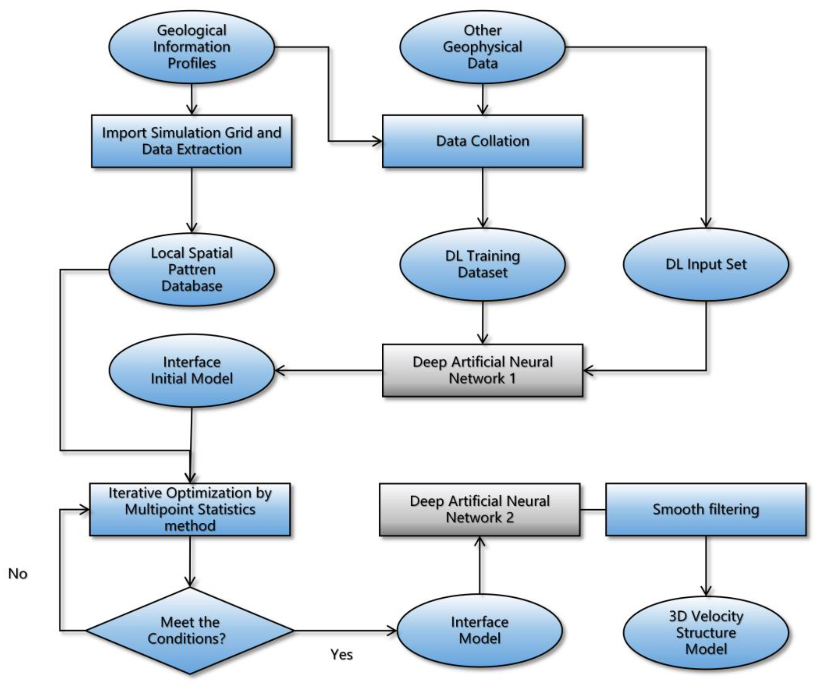
This study proposes a 3D geological stochastic reconstruction algorithm that combines deep learning with MPS. The algorithmic flow is shown in Figure 3. After preprocessing the data, we trained two groups of multimodal artificial neural networks. The first group was used to predict the geological layer interfaces and generate the initial model, R0. After optimizing R0 using MPS iteration, we obtained a refined model R1. This refinement helps in reducing artifacts and ensuring a more accurate representation of geological interfaces. Then, the second group of multimodal deep artificial neural networks was employed to predict the P-wave velocity values at each spatial node, further refining the crustal structure. The final step involved applying a smoothing filter to the output, yielding the final 3D P-wave velocity structure model, denoted as Rfinal.

3.1. Multimodal Deep Artificial Neural Network

The MFT model utilized in this study is a multimodal deep feed-forward fully connected artificial neural network. The architecture, inspired by an autoencoder, is depicted in Figure 4. This model takes spatial coordinates (x, y) or (h, x, y) along with the normalized values of multiple heterogeneous geophysical datasets corresponding to these coordinates as input. It comprises multiple hidden layers, with the number of artificial neurons progressively decreasing in each layer. Through multiple hidden layers, different input data are transformed into feature vectors, forming fusion vectors that integrate multi-source heterogeneous data within a data-driven framework. During the training process, backpropagation ensures the robust integration of multiple geophysical datasets by optimizing loss functions. Regularization techniques further mitigate overfitting, enhancing the model’s ability to generalize to unseen data. Through iterative optimization, the model continually adjusts its parameters to minimize the loss values, thereby improving its capacity to assimilate diverse data types. This methodology allows the model to fully exploit the benefits of various data sources, resulting in more accurate predictions.
Subsequently, similar to a decoder, additional hidden layers map these feature vectors back into geological information A(x, y) or A(h, x, y) corresponding to the spatial nodes (x, y) or (h, x, y), with the number of artificial neurons increasing layer by layer. The root mean squared error (RMSE) is used to calculate the loss between the predicted values A(x, y)′/A(h, x, y)′ obtained from the output layer and the label data A(x, y)/A(h, x, y).
In this study, we employ a hierarchical modeling strategy, utilizing two groups of multimodal deep neural networks with identical architectures to enhance the model’s ability to effectively capture and reconstruct the complex relationships between the input data and the target geological attributes.
The training process for the deep neural network is as follows:
(1)
Network Construction: Construct a multimodal deep neural network for the geological attributes that need to be reconstructed in 3D. The algorithm employs a feed-forward fully connected artificial neural network with nine hidden layers, comprising a total of 1,211,451 parameters;
(2)
Data Input: Input the training data into the deep neural network and set the training parameters. The training data A(x, y) or A(h, x, y) corresponding to spatial nodes (x, y) or (h, x, y) are compared with the predicted outputs A(x, y)′ or A(h, x, y)′;
(3)
Network Training: The loss values between the predicted and actual data are adjusted through backpropagation, updating the weights and biases of artificial neurons in each hidden layer. The simulation is limited to a maximum of 10,000 epochs. When the loss value stabilizes below a predefined threshold of 0.5 × 10⁻⁵, the training is terminated early, resulting in the corresponding deep neural network M.

3.2. Hierarchical Modeling Strategy

To effectively address the complexity of the SCS region’s internal structure and the sparsity of available data, a hierarchical modeling strategy was introduced. This approach involves dividing the task of generating unsampled P-wave velocity values into two separate tasks, each modeled using a distinct multimodal deep artificial neural network (Figure 5).
The first task focuses on simulating the geological layering structure of the crust based on multi-source heterogeneous data. The initial model R0 generated by the first set of deep neural networks includes the 3D spatial distribution of sedimentary layers (1.7–5.5 km/s), the upper crust (5.5–6.5 km/s), and the lower crust (6.5–8 km/s). Artificial artifacts in this initial model are then removed using an MPS optimization algorithm, resulting in the refined crustal structure model R1. The input data for this set of multimodal artificial neural networks consist of a multi-source heterogeneous dataset Bn(x,y) and two-dimensional spatial coordinates (x, y), while the corresponding label data represent the thickness values A(x, y) of the various geological layers at these planar coordinates (x, y). The steps for this process are:
(1)
Training Image Transformation: Traverse the TI and assign different layer attributes to each grid node based on the range of values at that node, generating a TI’ with layer attributes;
(2)
Layer Attribute Normalization: Use a window of size h × 1 × 1 to traverse the TI’ with layer attributes, simplifying the information at each depth plane coordinate node (x, y) into a sequence of thicknesses of the three geologic layers (sedimentary layer, upper crust, and lower crust). Normalize this sequence and use it as the label for the training dataset of the multimodal deep artificial neural network. The plane coordinate node (x, y) and the multi-source heterogeneous data Bn(x,y) corresponding to that node are used as inputs;
(3)
Network Training: Train the multimodal deep artificial neural network using the training dataset to predict the thicknesses of each geologic layer at a given coordinate node. This trained network is denoted as M1;
(4)
Initial Model Generation: Use M1 to predict the thicknesses of the sedimentary layer, upper crust, lower crust, and mantle for all unsampled plane coordinate nodes (x, y) in the simulation grid (SG). Based on these thicknesses and constraints from the topography and Moho depth, reconstruct the various layers in the SG and obtain the initial model R0;
(5)
Optimization: Combine the MPS iteration process to optimize R0 and obtain the refined crust structure model R1.
The second task is simulating the P-wave velocity structure in each geological layer based on multi-source heterogeneous data. Upon obtaining the refined interface model R1, the second group of multimodal deep artificial neural networks is employed to calculate the 3D P-wave velocity structure at the unsampled grid nodes between each geological interface. The final step requires integrating all models generated by the second set of neural networks to derive a comprehensive 3D crustal velocity structure model. The input data for this set of multimodal artificial neural networks consist of a multi-source heterogeneous dataset Bn(x,y) and three-dimensional spatial coordinates (x, y, z), while the corresponding label data represent the P-wave velocity values A(h, x, y) at these spatial coordinates (x, y, z). The steps for this process are:
(1)
Training Data Preparation: For each layer Qn, traverse the TI’ and origin TI to obtain the spatial nodes (h, x, y) with attributes corresponding to layer Qn and their corresponding P-wave velocity structure values from the assigned regions;
(2)
Training Dataset Construction: Use the spatial nodes (h, x, y) and the corresponding multi-source heterogeneous data Bn(x,y) as inputs. The values A(h, x, y) of the nodes serve as labels to construct the training dataset for the multimodal deep artificial neural networks;
(3)
Train the Second Group of Networks: Train the multimodal deep artificial neural networks with the training dataset to obtain the deep learning model MQn. This model is capable of predicting the P-wave velocity structure based on spatial coordinates and multi-source heterogeneous data;
(4)
Model Application: For each layer Qn, traverse the grid nodes in the refined crust structure model R1 with attributes corresponding to Qn. Use the coordinates (h, x, y) and their associated Bn(x,y) as inputs for the multimodal deep artificial neural network MQn, yielding the P-wave velocity structure at these nodes;
(5)
Final Model Synthesis: Repeat the above steps until all the unsampled nodes in each layer of the model are assigned values. After smoothing, the final model Rfinal of the 3D crustal velocity structure is obtained.

3.3. Multipoint Statistical Iterative Process

The results generated by the multimodal deep artificial neural network can be regarded as an initial implementation. However, directly generating models often results in discontinuities and artifacts, as deep learning does not optimize local spatial features during the simulation process. To address this, we adopt an expectation-maximization (EM) iteration procedure similar to GOSIM [13,89] to improve the simulation result R0R0. This iterative process includes enhancements in parallel optimization, optimal mode selection, and update rules. The Table S2 in Supplementary Materials provides a detailed outline of this process.

4. Results

The 3D crustal P-wave velocity structure model of the SCS was constructed using a simulation grid with dimensions of 70 × 400 × 400, totaling 11,200,000 grid cells. The modeling area covers the SCS region from 106° E to 122° E and 8° N to 24° N, with a vertical depth range extending from sea level to 35 km. The vertical grid spacing is 0.5 km per grid, and the horizontal grid spacing is 0.04° per grid. The artificial neural network was trained for 10,000 epochs. On a desktop computer, the complete model construction took approximately 30 h.
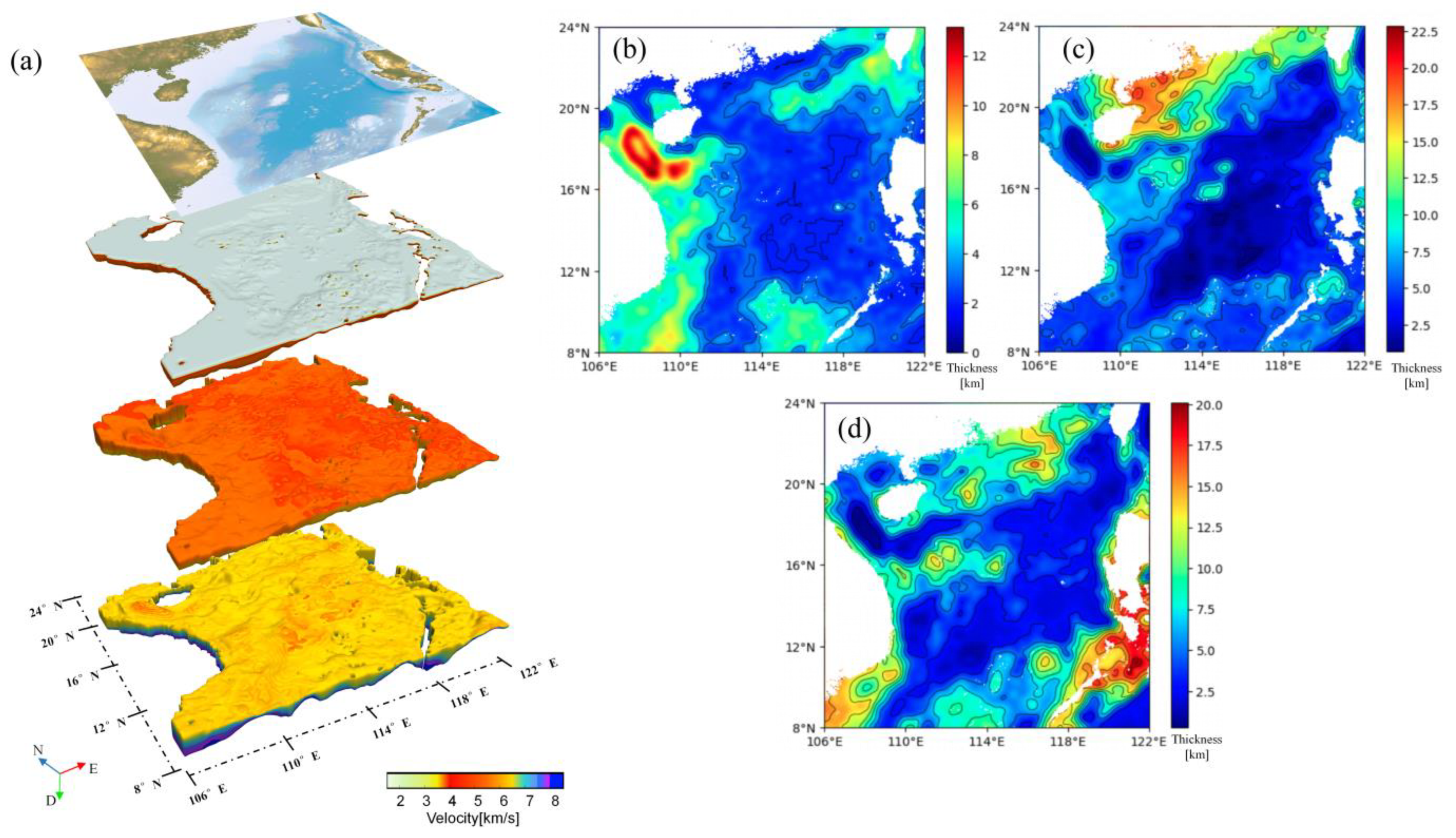
Figure 6 presents the thickness maps of the sedimentary layer, upper crust, and lower crust derived from the modeling results. The white areas represent regions without data, primarily on land. P-wave velocity structure profiles are concentrated in oceanic regions, where crustal velocity structures differ significantly from those on land. Consequently, we lack sufficient land samples for reliable deep learning predictions, necessitating further validation for these unsampled areas. Since our study focuses on the SCS, we have excluded land areas from the model. The average thickness of the sedimentary layer is 3.64 km, with a maximum thickness of 13.0 km. Regions with relatively large thicknesses are concentrated near the Yinggehai Basin (Figure 6b). The average thickness of the upper crust is 6.95 km, while the average thickness of the lower crust is 7.0 km. A clear thinning phenomenon was observed in the SCS basin, with minimum thicknesses of 0.5 km and 1.0 km, respectively (Figure 6c,d).
Figure 7 shows the modeling results for the sedimentary layer interface, Moho interface, top crust interface, and their respective depth distributions. The results indicate that the average depth of the sedimentary layer interface in the SCS basin is approximately 1.61 km, with a maximum depth reaching 5.0 km. The top crust interface exhibits similar characteristics, with an overall average depth of 5.24 km. The deepest point is located near the Yinggehai Basin, where the depth reaches 14.0 km. The Moho interface is relatively shallow within the SCS basin but deepens in other regions, with an overall average depth of 21.0 km. Moving from the peripheral regions to the central basin, the Moho interface depth decreases sharply from around 20 km to approximately 10 km. Overall, the 3D crustal model of the SCS aligns well with previous studies concerning the velocity structure.

5. Discussion

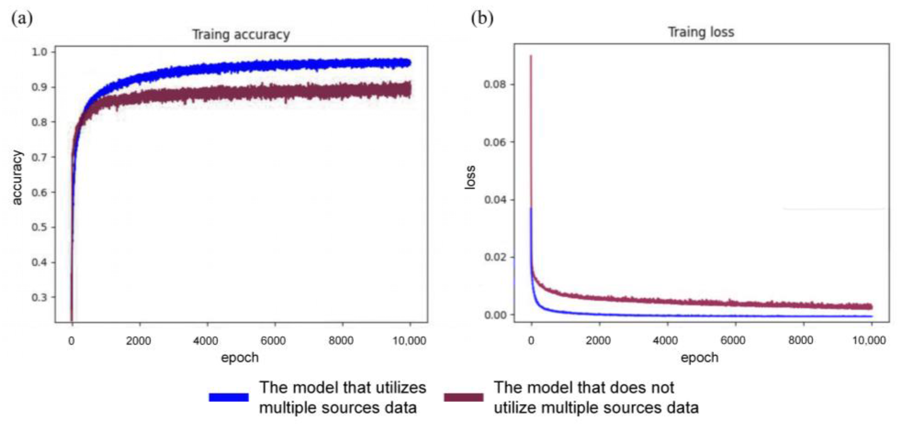
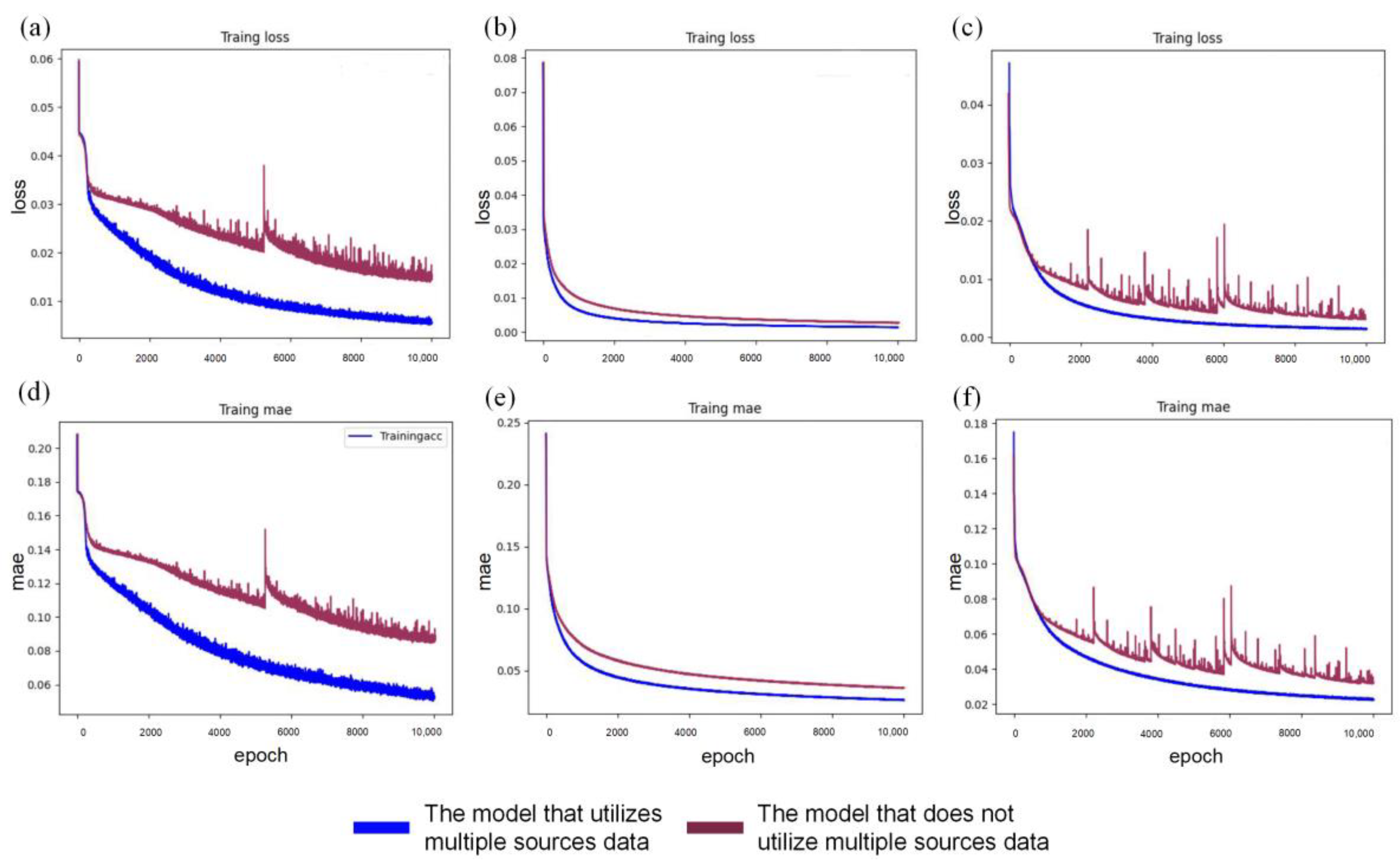
In this study, deep learning was used to explore the mapping between different geophysical data, spatial locations, and velocity structure values. This process was automatically achieved through backpropagation. By comparing the training and prediction performance of models using multi-source heterogeneous data with those that do not, under the same deep learning framework, the benefits of the integration of multi-source heterogeneous data are highlighted. As illustrated in Figure 8 and Figure 9, the deep learning neural network trained with multi-source heterogeneous data demonstrates significantly improved performance, reflected by lower loss values, higher accuracy, and a reduction in the average absolute error in predicting velocity structures. Additionally, these models require fewer training iterations to achieve a stable state. When compared with the curves of loss values, error rates, and accuracy obtained without integrating multi-source heterogeneous data, the incorporation of such data results in reduced fluctuation ranges in these curves.
Furthermore, we calculated several goodness-of-fit parameters for the model. With the use of multi-source heterogeneous data, the model achieved a goodness-of-fit value of 0.96029, surpassing the 0.95717 value obtained without such data. The prediction results indicate a mean squared error (MSE) of 0.16505, mean absolute error (MAE) of 0.15696, and mean absolute percentage error (MAPE) of 0.0307. Compared with the results from models that did not utilize heterogeneous data, these values represent reductions of 0.01151, 0.00915, and 0.00213, respectively. These findings demonstrate that the model excels in reducing errors and significantly enhances the prediction accuracy. Overall, the results indicate that the multimodal deep artificial neural network architecture developed in this study effectively integrates diverse geophysical data from the SCS, thereby substantially improving the performance of 3D geological information modeling algorithms.
To verify the accuracy of the model, the multi-source heterogeneous data fusion model developed in this study (Figure 10a–c) was compared with several other models (one constructed without using multi-source heterogeneous data (Figure 10d–f), the Kriging interpolation model (Figure 10g–i), and the MPS interpolation model (Figure 10j–l). Visually, the Kriging interpolation result appears excessively smooth, lacking local details, and shows significant discrepancies in terrain variations and the Moho depth compared with existing models, as well as numerous artificial artifacts. In contrast, the models constructed without multi-source heterogeneous data and the one using MPS both exhibit substantial discontinuities and abrupt thickenings in the upper and lower crust. The model generated by MPS also displays stratigraphic misalignments, which are clearly inconsistent with established geological knowledge. Overall, these comparisons highlight the superior performance of the multi-source heterogeneous data fusion model developed in this study, which more accurately captures the complexities of the geological structures in the SCS. A detailed comparison of the methods can be found in the Supplementary Materials.
Excluding the OBS2017-2 data [84], we constructed and compared the four types of models mentioned earlier by extracting profiles at that specific location (Figure 11). The residuals between the profile generated by the multi-source heterogeneous data fusion model (Figure 11c) and the OBS2017-2 data were calculated, resulting in a root mean square error (RMSE) of 0.6281 km/s and a Jensen–Shannon divergence (JS divergence) of 0.03484. For the profile from the model without integrating multi-source heterogeneous data (Figure 11e), the RMSE was 0.8246 km/s and the JS divergence was 0.05443. The Kriging interpolation model (Figure 11g) exhibited an RMSE of 0.8723 km/s and a JS divergence of 0.05881. These results indicate that the latter three models deviate more significantly from the actual conditions. Similarly, comparisons excluding OBS2012-2 and OBS973-2 data are presented in the Supplementary Materials (Figures S5 and S6), further verifying that the model constructed using the algorithm proposed in this study is closer to the real geological conditions.
Attribute proportion statistics quantify the relative distribution of different geological attributes within the model, providing an intuitive measure of the discrepancies between the modeling results and known geological data. Figure S7 presents a comparison of attribute proportions across various geological layers in the 3D model categorized by velocity. The results indicate that the new modeling method yields attribute proportions that more closely align with the known data compared with those obtained using the Kriging interpolation and MPS methods. Additionally, the inclusion or exclusion of multi-source heterogeneous data appears to have a minimal impact on the attribute proportions in the simulation results.
By calculating various metrics such as the average thickness of the geological layers (Figure 12a), maximum thickness (Figure 12b), minimum thickness (Figure 12c), average elevation of the top surface (Figure 12d), maximum elevation of the top surface (Figure 12e), minimum elevation of the top surface (Figure 12f), average elevation of the bottom surface (Figure 12g), maximum elevation of the bottom surface (Figure 12h), and minimum elevation of the bottom surface (Figure 12i), we can visually assess the similarities and differences between the simulation results and the known data at the geological layer level. The traditional Kriging interpolation method tends to represent geological interfaces as smooth curved surfaces, leading to simulations where the top surfaces of the geological layers are generally shallower and the bottom surfaces deeper than expected. In contrast, the modeling results obtained by integrating multi-source heterogeneous data show greater alignment with the training data in terms of these statistical indicators, and they more accurately reflect the actual geological conditions compared with the Kriging interpolation model, the MPS interpolation model, and the simulation results that do not utilize multi-source heterogeneous data.
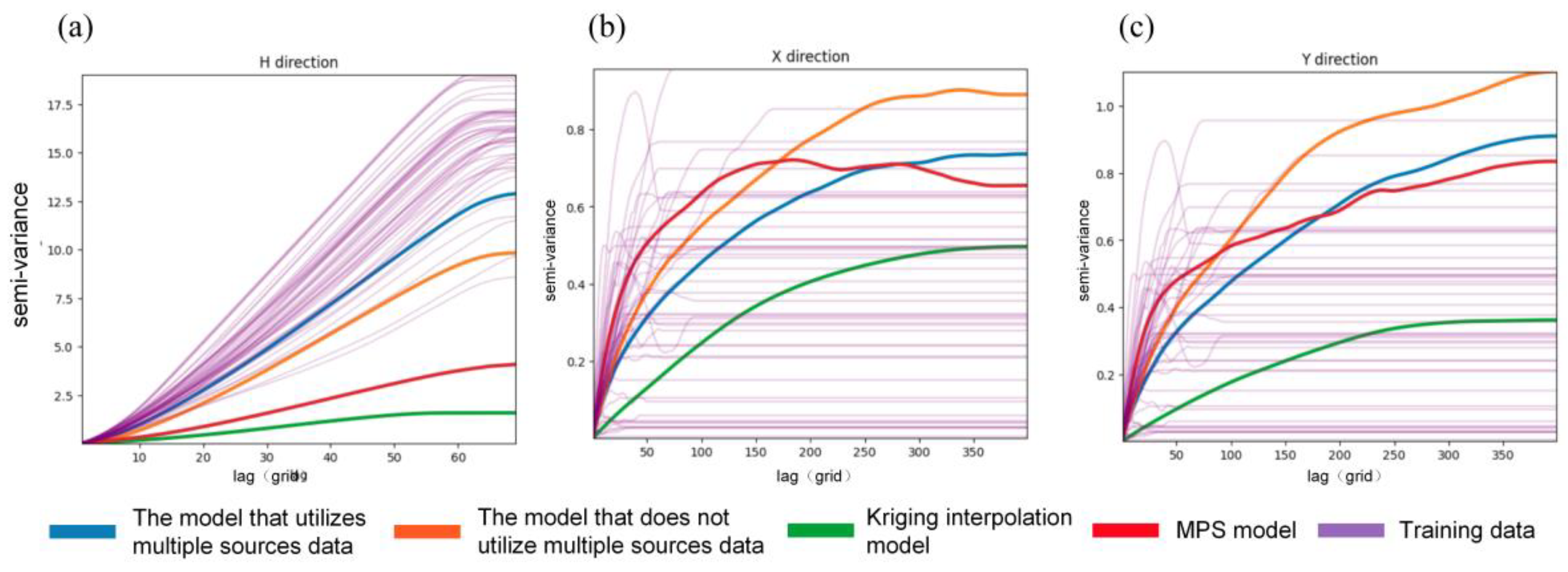
The variogram function is a powerful tool for capturing and representing the spatial structure and randomness of regionalized variables [90,91]. As illustrated in Figure 13, the variogram curves of the modeling results that incorporate multi-source heterogeneous data are centrally positioned within the set of variogram curves derived from 44 forward profiles. This indicates that the variogram curves of the models developed using multi-source heterogeneous data more closely resemble those of the training data compared with other methods.
Although the deep learning model captures the overall trends, it still exhibits some artificial artifacts and discontinuities (Figure 14a), highlighting the steep velocity transition. These observations indicate that, while the proposed deep artificial neural network effectively captures the global spatial characteristics of known geological features, it lacks the precision needed to accurately characterize local spatial features. In contrast, the iterative MPS algorithm substantially reduces or eliminates these artificial artifacts (Figure 14b). The MPS method provides a finer local characterization by leveraging the local spatial features obtained from the training images (TIs), while also correcting some local errors, leading to a more accurate and reliable 3D geological model.
By visually inspecting and comparing the geological statistical parameters and profile sections, we can preliminarily conclude that the 3D crustal velocity structure model of the SCS developed in this study is reasonably reliable and offers substantial improvements over traditional 3D models constructed using Kriging interpolation, models that do not utilize heterogeneous multi-source data, and models constructed with MPS alone. The proposed model successfully reconstructs the global spatial characteristics of the crustal P-wave velocity structure (Figure 15), aligning well with prior knowledge of the SCS region. It demonstrates better consistency with the original data in terms of attribute proportions, variogram statistics, geological interface elevation, and thickness statistics.
During the 3D random simulation process, the availability of conditional data directly influences the diversity of spatial distribution patterns. The more data we have, the greater the constraints imposed on the simulation by known information, which brings the model closer to reality. Multimodal deep artificial neural networks, when trained with larger datasets or additional modalities, exhibit superior generalization and stability. Additionally, an increased amount of target modeling data offers more local spatial patterns for multipoint statistics, enabling the 3D geological model to better capture local spatial features that correspond to real-world conditions during iterative optimization. By incorporating more heterogeneous data from various sources, the proposed algorithm can continually update, calibrate, and refine previously constructed 3D geological models, thereby enhancing their adaptability to new data distributions.
It is worth noting that the data used to train the multimodal deep artificial neural network in this study were not limited to data from the SCS region. In subsequent work, it could be beneficial to use data from other regions, such as seismic exploration profiles and geophysical data from land and other oceanic regions, to provide references for constructing geological models in the SCS. Different regions may share similarities and correlations in geological conditions, offering valuable insights for building higher-quality models. Theoretically, the use of cross-regional data can improve the accuracy and generalization capabilities of deep artificial neural networks, allowing the algorithm to extract and summarize more universal geological features or patterns from the data. This, in turn, enhances the algorithm’s understanding and predictive ability regarding the geological conditions of the study area. Due to the lack of waveform data covering the entire SCS region, traditional geophysical validation methods (like checkerboard tests) are difficult to implement. Therefore, we used statistical methods commonly applied in 3D modeling to validate the differences between our constructed model and known data. This approach ensures the model’s reliability and credibility.
In addition to the P-wave velocity structure, other geological attributes can also be used as target modeling data for this algorithm, such as S-wave velocity structures and density structures. By collecting and organizing these data into comprehensive datasets, this algorithm has the potential to construct corresponding 3D models of various geophysical or geological attributes. The construction of these models can provide foundational information for a wide range of applications, including geological research, resource exploration, seismic activity monitoring, and studies on Earth’s evolutionary processes.

6. Conclusions

In this study, we introduced a novel 3D modeling technique that integrates multimodal deep learning with multipoint statistics (MPS) to construct a detailed crustal P-wave velocity structure model of the SCS. Our approach effectively addresses the challenges associated with reconstructing non-stationary features of geological structures and integrating heterogeneous data from multiple sources. By leveraging multimodal deep learning, we were able to amalgamate diverse data sources, enhancing the precision of 3D model construction and minimizing modeling ambiguities. This method is a powerful supplement to traditional forward and inverse waveform methods. It combines the advantages of deep learning technology to enable effective modeling of subsurface structures even when the data are insufficient to support comprehensive waveform inversion.
The hierarchical modeling strategy employed in the process simplifies the training of deep learning networks, ensuring that the final model accurately captures both local and global spatial features. The model constructed using this novel approach was validated against traditional methods, showing superior performance in terms of alignment with prior knowledge and the original data.
The 3D crustal P-wave velocity structure model of the SCS developed in this study provides an intuitive and reliable representation of the spatial distribution characteristics of geological structures within the region. It offers a robust data foundation for researchers to gain a more comprehensive understanding of the tectonic evolution, dynamic mechanisms, resource exploration, and other related geological studies in the SCS. Additionally, this model can serve as an initial model for 3D travel-time inversion of real data and guide future survey design.
Our findings demonstrate that the integration of multimodal deep learning and MPS into geological modeling not only enhances model accuracy and reliability but also opens new avenues for the application of data-driven approaches in geoscience research. As we continue to gather and incorporate more diverse and comprehensive datasets, the potential for refining and expanding our understanding of Earth’s subsurface structures through advanced modeling techniques will only increase.

Supplementary Materials

The following supporting information can be downloaded at: https://www.mdpi.com/article/10.3390/jmse12111907/s1, Figure S1: The modeling results of the SCS structure model constructed by integrating multi-source heterogeneous data. (a) is the overall 3D velocity structure model. (b) represents the result of modeling for the sedimentary layer, (c) for the upper crust, and (d) and (e) respectively represent the lower crust and mantle in the modeling results; Figure S2: The modeling results of the SCS model constructed without integrating multi-source heterogeneous data. (a) is the overall 3D velocity structure model. (b) represents the result of modeling for sedimentary layer, (c) for the upper crust, and (d) and (e) respectively represent the lower crust and Mantle in the modeling results; Figure S3 The modeling results of the SCS model constructed by Kriging interpolation. (a) is the overall 3D velocity structure model. (b) represents the result of modeling for the sedimentary layer, (c) for the upper crust, and (d) and (e) respectively represent the lower crust and Mantle in the modeling results; Figure S4 The modeling results of the SCS model constructed by Multipoint statistics. (a) is the overall 3D velocity structure model. (b) represents the result of modeling for the sedimentary layer, (c) for the upper crust, and (d) and (e) respectively represent the lower crust and Mantle in the modeling results; Figure S5 (a) OBS2012-2 forward modeling profile. (b) Schematic diagram of the location of OBS2012-2 profile data, where the red line represents the OBS2012-2 profile.(c) (e) (g) are the profiles of OBS2012-2 position in the model constructed by using multi-source heterogeneous data, not using multi-source heterogeneous data, and Kriging interpolation respectively, and (d) (f) (h) are the residual maps of these profiles and OBS2012-2 profile data; Figure S6 (a) OBS973-2 forward modeling profile. (b) Schematic diagram of the location of OBS973-2 profile data, where the red line represents the OBS973-2 profile.(c) (e) (g) are the profiles of OBS973-2 position in the model constructed by using multi-source heterogeneous data, not using multi-source heterogeneous data, and Kriging interpolation respectively, and (d) (f) (h) are the residual maps of these profiles and OBS973-2 profile data; Figure S7 Comparison of attribute proportions; Table S1: The 44 crustal structure profiles data source list; Table S2: EM Iteration Algorithm Process.

Author Contributions

H.L. was responsible for developing the methodologies, processing data, programming algorithms, drawing figures, and drafting the initial manuscript. S.X. provided the central research ideas and overall planning, guided the methodologies and results, managed the data and project, secured funding, and wrote and revised the manuscript. C.F. participated in discussions regarding the methodologies and results and also contributed to revising the initial draft. C.Z. also engaged in the method and result discussions and made revisions to the initial draft. All authors have read and agreed to the published version of the manuscript.

Funding

This research was funded by the National Key Research and Development Program of China (2022YFC3102200), the National Natural Science Foundation of China (42076071), the Guangdong Basic and Applied Basic Research Foundation (2022A1515012019), the Special Fund of South China Sea Institute of Oceanology of the Chinese Academy of Sciences (SCSIO2023QY06) and the Natural Science Foundation of Hainan Province of China (423QN335).

Institutional Review Board Statement

This study does not involve ethical issues and does not require ethical approval.

Informed Consent Statement

Not applicable.

Data Availability Statement

The 44 OBS wide-angle seismic structure profiles are available through Yan et al., 2001, Fan et al., 2017, 2019, Wang et al., 2006, Wu et al., 2012, Ao et al., 2012, Wei et al., 2011, Cao et al., 2014, Zhu et al., 2018, Huang et al., 2011, 2021, Xia et al., 2018, 2022, Wan et al. 2017, Guo et al. 2016, Li et al. 2017, Liu et al. 2018, Hou et al., 2019, Zhang et al., 2023, Li et al., 2020, Li et al., 2021, Wang et al., 2022, Zhao et al., 2022, Yu et al., 2017, Wei et al., 2015, Liu et al., 2021, Guo et al., 2022; Pichot et al., 2014, Zhang et al., 2016, Xiong et al., 2018, Zhao et al., 2018, Lester et al., 2014, and Nissen et al., 1995 [43,53,54,55,56,57,58,59,60,61,62,63,64,65,66,67,68,69,70,71,72,73,74,75,76,77,78,79,80,81,82,83,84]. The IGPP Global Free Air Gravity Anomaly Data_01m is available through Pavlis et al., 2012 and Sandwell et al., 2021 [85,86], the EMAG2 Global Magnetic Anomaly Model_02m through Meyer et al., 2016 [87], and the SRTM+ Global Topography Data_01m through Tozer et al., 2019 [88].

Acknowledgments

Thanks go to the MAGMAN group for their suggestions and discussions on this research work. Meanwhile, we would like to extend my heartfelt thanks to the editor and the three reviewers for their valuable suggestions and hard work in improving the paper. Your insights and constructive feedback have greatly enhanced the quality of our manuscript, and we truly appreciate your efforts.

Conflicts of Interest

The authors declare no conflicts of interest.

References

  1. Lindsay, M.D.; Aillères, L.; Jessell, M.W.; de Kemp, E.A.; Betts, P.G. Locating and quantifying geological uncertainty in three-dimensional models: Analysis of the Gippsland Basin, southeastern Australia. Tectonophysics 2012, 546, 10–27. [Google Scholar] [CrossRef]
  2. Yin, Y.; Zhang, C.; Li, J.; Shi, S.Y. Progress and prospect of multiple-point geostatistics. J. Palaeogeogr. 2011, 13, 245–252. [Google Scholar]
  3. Kaufmann, O.; Martin, T. 3D geological modelling from boreholes, cross-sections and geological maps, application over former natural gas storages in coal mines. Comput. Geosci. 2008, 3, 278–290. [Google Scholar] [CrossRef]
  4. Ma, B.; Wu, S.; Mi, L.; Lüdmann, T.; Gao, J.; Gao, W. Mixed Carbonate-Siliciclastic Deposits in a Channel Complex in the Northern South China Sea. J. Earth Sci. 2018, 29, 707–720. [Google Scholar] [CrossRef]
  5. Qu, H.; Pan, M.; Liu, X. Urban 3-D geological modeling and its application to urbanization. Geol. Bull. China 2015, 34, 1350–1358. [Google Scholar]
  6. Zhang, J.; Wu, Q.; Hao, D. Framework for mine-water inrush scene constructing and drilling trajectory planning: A case study in the Zijiang Coal Mine, China. Arab. J. Geosci. 2019, 12, 499. [Google Scholar] [CrossRef]
  7. Song, W.; Yao, J.; Ma, J.; Couples, G.D.; Li, Y.; Sun, H. Pore-scale numerical investigation into the impacts of the spatial and pore-size distributions of organic matter on shale gas flow and their implications on multiscale characterisation. Fuel 2018, 216, 707–721. [Google Scholar] [CrossRef]
  8. Li, Y.; Teng, Q.; He, X.; Feng, J.; Xiong, S. Super-dimension-based three-dimensional nonstationary porous medium reconstruction from single two-dimensional image. J. Pet. Sci. Eng. 2019, 174, 968–983. [Google Scholar] [CrossRef]
  9. Mariethoz, G.; Renard, P.; Straubhaar, J. The direct sampling method to perform multiple-point geostatistical simulations. Water Resour. Res. 2010, 46. [Google Scholar] [CrossRef]
  10. Hou, W.; Chen, Y.; Liu, H.; Xiao, F.; Liu, C.; Wang, D. Reconstructing Three-dimensional geological structures by the Multiple-point statistics method coupled with a deep neural network: A case study of a metro station in Guangzhou, China. Tunn. Undergr. Space Technol. 2023, 136, 105089. [Google Scholar] [CrossRef]
  11. Guardiano, F.B.; Srivastava, R.M. Multivariate geostatistics: Beyond bivariate moments. In Geostatistics Tróia’92; Springer: Dordrecht, The Netherlands, 1993; Volume 1, pp. 133–144. [Google Scholar]
  12. Yu, S.Y.; Li, S.H.; He, Y.B.; Duan, T.Z.; Lian, P.Q.; Tao, J.Y.; Bao, X. Multiple-point geostatistics algorithm based on pattern scale-down cluster. Acta Pet. Sin. 2016, 37, 1403. [Google Scholar]
  13. Arpat, G.B.; Caers, J. Conditional simulation with patterns. Math. Geol. 2007, 39, 177–203. [Google Scholar] [CrossRef]
  14. Yang, L.; Hou, W.; Cui, C.; Cui, J. GOSIM: A multi-scale iterative multiple-point statistics algorithm with global optimization. Comput. Geosci. 2016, 89, 57–70. [Google Scholar] [CrossRef]
  15. Tahmasebi, P.; Sahimi, M.; Caers, J. MS-CCSIM: Accelerating pattern-based geostatistical simulation of categorical variables using a multi-scale search in Fourier space. Comput. Geosci. 2014, 67, 75–88. [Google Scholar] [CrossRef]
  16. Honarkhah, M.; Caers, J. Stochastic simulation of patterns using distance-based pattern modeling. Math. Geosci. 2010, 42, 487–517. [Google Scholar] [CrossRef]
  17. Zhang, T.; Switzer, P.; Journel, A. Filter-based classification of training image patterns for spatial simulation. Math. Geol. 2006, 38, 63–80. [Google Scholar] [CrossRef]
  18. Pourfard, M.; Abdollahifard, M.J.; Faez, K.; Motamedi, S.A.; Hosseinian, T. PCTO-SIM: Multiple-point geostatistical modeling using parallel conditional texture optimization. Comput. Geosci. 2017, 102, 116–138. [Google Scholar] [CrossRef]
  19. Strebelle, S. Conditional simulation of complex geological structures using multiple-point statistics. Math. Geol. 2002, 34, 1–21. [Google Scholar] [CrossRef]
  20. Straubhaar, J.; Renard, P.; Mariethoz, G.; Froidevaux, R.; Besson, O. An improved parallel multiple-point algorithm using a list approach. Math. Geosci. 2011, 43, 305–328. [Google Scholar] [CrossRef]
  21. Dimitrakopoulos, R.; Mustapha, H.; Gloaguen, E. High-order statistics of spatial random fields: Exploring spatial cumulants for modeling complex non-gaussian and non-linear phenomena. Math. Geosci. 2010, 42, 65–99. [Google Scholar] [CrossRef]
  22. Yao, L.; Dimitrakopoulos, R.; Gamache, M. Learning high-order spatial statistics at multiple scales: A kernel-based stochastic simulation algorithm and its implementation. Comput. Geosci. 2021, 149, 104702. [Google Scholar] [CrossRef]
  23. De Vries, L.M.; Carrera, J.; Falivene, O.; Gratacós, O.; Slooten, L.J. Application of multiple point geostatistics to non-stationary images. Math. Geosci. 2009, 41, 29–42. [Google Scholar] [CrossRef]
  24. Chen, G.X.; Zhao, F.; Wang, J.G.; Zheng, H.B.; Yan, Y.Z.; Wang, A.P.; Li, J.Y.; Hu, Y.P. Regionalized multiple-point stochastic geological modeling: A case from braided delta sedimentary reservoirs in Qaidam Basin, NW China. Pet. Explor. Dev. 2015, 42, 697–704. [Google Scholar] [CrossRef]
  25. Straubhaar, J.; Renard, P. Conditioning Multiple-Point Statistics Simulation to Inequality Data. Earth Space Sci. 2021, 8, e2020EA001515. [Google Scholar] [CrossRef]
  26. Hansen, T.M.; Le, T.V.; Mosegaard, K.; Cordua, K.S. Multiple point statistical simulation using uncertain (soft) conditional data. Comput. Geosci. 2018, 114, 1–10. [Google Scholar] [CrossRef]
  27. Wang, M.C.; Shang, X.F.; Duan, T.Z. A review of the establishment methods of training image in multiple-point statistics modeling. Geol. J. China Univ. 2022, 28, 96. [Google Scholar]
  28. Minar, M.R.; Naher, J. Recent advances in deep learning: An overview. arXiv 2018, arXiv:1807.08169. [Google Scholar]
  29. Hinton, G.E.; Salakhutdinov, R.R. Reducing the dimensionality of data with neural networks. Science 2006, 313, 504–507. [Google Scholar] [CrossRef] [PubMed]
  30. Li, T.; Zuo, R.; Xiong, Y.; Peng, Y. Random-drop data augmentation of deep convolutional neural network for mineral prospectivity mapping. Nat. Resour. Res. 2021, 30, 27–38. [Google Scholar] [CrossRef]
  31. LeCun, Y.; Bengio, Y.; Hinton, G. Deep learning. Nature 2015, 521, 436–444. [Google Scholar] [CrossRef]
  32. Adler, A.; Araya-Polo, M.; Poggio, T. Deep learning for seismic inverse problems: Toward the acceleration of geophysical analysis workflows. IEEE Signal Process. Mag. 2021, 38, 89–119. [Google Scholar] [CrossRef]
  33. Ngiam, J.; Khosla, A.; Kim, M.; Nam, J.; Lee, H.; Ng, A.Y. Multimodal deep learning. In Proceedings of the 28th International Conference on Machine Learning (ICML), Bellevue, WA, USA, 28 June–2 July 2011. [Google Scholar]
  34. Bergado, J.R.; Persello, C.; Reinke, K.; Stein, A. Predicting wildfire burns from big geodata using deep learning. Saf. Sci. 2021, 140, 105276. [Google Scholar] [CrossRef]
  35. Zhang, C.; Zuo, R.; Xiong, Y. Detection of the multivariate geochemical anomalies associated with mineralization using a deep convolutional neural network and a pixel-pair feature method. Appl. Geochem. 2021, 130, 104994. [Google Scholar] [CrossRef]
  36. Zhang, K.; Yu, H.Q.; Ma, X.P.; Zhang, J.D.; Wang, J.; Yao, C.J.; Yao, J. Multi-source information fused generative adversarial network model and data assimilation based history matching for reservoir with complex geologies. Pet. Sci. 2022, 19, 707–719. [Google Scholar] [CrossRef]
  37. Chen, Q.; Liu, G.; Ma, X.; Li, X.; He, Z. 3D stochastic modeling framework for quaternary sediments using multiple-point statistics: A case study in Minjiang Estuary area, southeast China. Comput. Geosci. 2020, 136, 104404. [Google Scholar] [CrossRef]
  38. Cui, Z.; Chen, Q.; Liu, G. Characterization of subsurface hydrogeological structures with convolutional conditional neural processes on limited training data. Water Resour. Res. 2022, 58, e2022WR033161. [Google Scholar] [CrossRef]
  39. Li, L.; Srinivasan, S.; Zhou, H.; Gómez-Hernández, J.J. Simultaneous estimation of geologic and reservoir state variables within an ensemble-based multiple-point statistic framework. Math. Geosci. 2014, 46, 597–623. [Google Scholar] [CrossRef]
  40. Taylor, B.; Hayes, D.E. Origin and History of the South China Sea Basin; Washington DC American Geophysical Union Geophysical Monograph Series; American Geophysical Union: Washington, DC, USA, 1983; Volume 27, pp. 23–56. [Google Scholar]
  41. Piao, Q.F.; Zhang, B.; Zhang, R.; Geng, M.; Zhong, G. Continent-ocean transition in the northern South China Sea by high-quality deep reflection seismic data. Chin. J. Geophys. 2022, 65, 2546–2559. [Google Scholar]
  42. Liu, G.D. Intensify the research on continental margin of South China Sea. Chin. J. Geophys. 2011, 54, 2991–2992. [Google Scholar]
  43. Xia, S.; Zhao, F.; Zhao, D.; Fan, C.; Wu, S.; Mi, L.; Wan, K. Crustal plumbing system of post-rift magmatism in the northern margin of South China Sea: New insights from integrated seismology. Tectonophysics 2018, 744, 227–238. [Google Scholar] [CrossRef]
  44. Xie, X.; Zhao, S.; Ren, J.; Yang, Y.; Yao, Y. Marginal Sea Closure Process and Genetic Mechanism of South China Sea during Post-Spreading Period. Earth Sci. 2022, 47, 3524–3542. [Google Scholar]
  45. Wu, S.; Zhang, G.; Huang, Y.; Liang, J.; Wong, H.K. Gas hydrate occurrence on the continental slope of the northern South China Sea. Mar. Pet. Geol. 2005, 22, 403–412. [Google Scholar] [CrossRef]
  46. Wang, X.; Hutchinson, D.R.; Wu, S.; Yang, S.; Guo, Y. Elevated gas hydrate saturation within silt and silty clay sediments in the Shenhu area, South China Sea. J. Geophys. Res. Solid Earth 2011, 116. [Google Scholar] [CrossRef]
  47. Xu, Z.; Hu, T.; Pang, X.Q.; Wang, E.Z.; Liu, X.H.; Wu, Z.Y.; Wang, T. Research progress and challenges of natural gas hydrate resource evaluation in the South China Sea. Pet. Sci. 2022, 19, 13–25. [Google Scholar] [CrossRef]
  48. Cin, M.D.; Bhm, G.; Busetti, M.; Picotti, S.; Zgur, F.; Camerlenghi, A. 3d velocity-depth model from multichannel seismic in the dinaric foredeep of the gulf of trieste (adriatic sea), at the ne edge of adria plate. Tectonophysics 2022, 838, 229470. [Google Scholar]
  49. Jian-Ping, W.U.; Ting, Y.; Wei-Lai, W.; Yue-Hong, M.; Tian-Zhong, Z. Three-dimensional p-wave velocity structure around the xiaojiang fault zone and its tectonic implications. Chin. J. Geophys. 2013, 56, 400–410. [Google Scholar] [CrossRef]
  50. Yuan, Y.; He, E.; Zhao, M.; Zhang, C.; Gao, J.; Zhang, J.; Sun, Z. Seismic velocity structure and tectonic evolution of the continent-ocean transition in the mid-northern South China sea. Tectonophysics 2023, 862, 229984. [Google Scholar] [CrossRef]
  51. Tian, D.; Liu, X. Identification of gas hydrate based on velocity cross plot analysis. Mar. Geophys. Res. 2021, 42, 11. [Google Scholar] [CrossRef]
  52. Singh, B.; Malinowski, M. Seismic imaging of mineral exploration targets: Evaluation of ray- vs. wave-equation-based pre-stack depth migrations for crooked 2d profiles. Minerals 2023, 13, 264. [Google Scholar] [CrossRef]
  53. Yan, P.; Liu, Z.; Zhou, D. A crustal structure profile across the northern continental margin of the south china sea. Tectonophys. Int. J. Geotecton. Geol. Phys. Inter. Earth 2001, 338, 1–21. [Google Scholar]
  54. Fan, C.; Xia, S.; Zhao, F.; Sun, J.; Cao, J.; Xu, H.; Wan, K. New insights into the magmatism in the northern margin of the South China Sea: Spatial features and volume of intraplate seamounts. Geochem. Geophys. Geosyst. 2017, 18, 2216–2239. [Google Scholar] [CrossRef]
  55. Fan, C.; Xia, S.; Cao, J.; Zhao, F.; Sun, J.; Wan, K.; Xu, H. Lateral crustal variation and post-rift magmatism in the northeastern South China Sea determined by wide-angle seismic data. Mar. Geol. 2019, 410, 70–87. [Google Scholar] [CrossRef]
  56. Wang, T.K.; Chen, M.K.; Lee, C.S.; Xia, K. Seismic imaging of the transitional crust across the northeastern margin of the South China Sea. Tectonophysics 2006, 412, 237–254. [Google Scholar] [CrossRef]
  57. Wu, Z.L.; Li, J.B.; Ruan, A.G.; Lou, H.; Ding, W.W.; Li, N.X. Crustal structure of the northwestern sub-basin, South China Sea: Results from a wide-angle seismic experiment. Sci. China Earth Sci. 2012, 55, 159–172. [Google Scholar] [CrossRef]
  58. Ao, W.; Zhao, M.H.; Qiu, X.L.; Ruan, A.; Li, J. Crustal structure of the. Northwest Sub-Basin of the South China Sea and its tectonic implication. Earth Sci.-J. China Univ. Geosci. 2012, 37, 779–790. [Google Scholar]
  59. Wei, X.; Ruan, A.; Zhao, M.; Qiu, X.; Wu, Z.; Niu, X. Shear wave velocity structure of Reed Bank, southern continental margin of the South China Sea. Tectonophysics 2015, 644, 151–160. [Google Scholar] [CrossRef]
  60. Cao, J.H.; Sun, J.L.; Xu, H.L.; Xia, S.H. Seismological features of the littoral fault zone in the Pearl River Estuary. Chin. J. Geophys. 2014, 57, 498–508. [Google Scholar]
  61. Zhu, J.; Xu, H.; Qiu, X.; Ye, C.; Li, S. Crustal structure and rifting of the northern South China Sea margin: Evidence from shoreline-crossing seismic investigations. Geol. J. 2018, 53, 2065–2083. [Google Scholar] [CrossRef]
  62. Huang, H.B.; Qiu, X.L.; Xu, H.L.; Zhao, M.H.; Hao, T.Y.; Xu, Y.; Li, J.B. Preliminary results of the earthquake observation and the onshore-offshore seismic experiments on Xisha Block. Chin. J. Geophys. 2011, 54, 3161–3170. [Google Scholar]
  63. Huang, H.; Klingelhoefer, F.; Qiu, X.; Li, Y.; Wang, P. Seismic Imaging Of an Intracrustal Deformation In the Northwestern Margin Of the South China Sea: The Role Of a Ductile Layer In the Crust. Tectonics 2021, 40, e2020TC006260. [Google Scholar] [CrossRef]
  64. Xia, S.; Fan, C.; Wang, D.; Cao, J.; Zhao, F. Hyperextended crustal structure of the Qiongdongnan Basin and subsequent magmatic influence from the Hainan mantle plume. Sci. China Earth Sci. 2022, 65, 845–862. [Google Scholar] [CrossRef]
  65. Wan, K.; Xia, S.; Cao, J.; Sun, J.; Xu, H. Deep seismic structure of the northeastern South China Sea: Origin of a high-velocity layer in the lower crust. J. Geophys. Res. Solid Earth 2017, 122, 2831–2858. [Google Scholar] [CrossRef]
  66. Guo, X.R.; Zhao, M.H.; Huang, H.B.; Qiu, X.L.; Zhang, J.Z. Crustal structure of xisha block and its tectonic attributes. Chin. J. Geophys. 2016, 59, 288–300. [Google Scholar]
  67. Li, Y.Q.; Yan, P.; Wang, Y.L.; Zhong, G.J. Deep crustal structure revealed by ocean bottom seismic profile OBS2015-1 in southwestern Dongsha waters. J. Trop. Oceanogr. 2017, 36, 83–92. [Google Scholar]
  68. Liu, S.Q.; Zhao, M.H.; Sibuet, J.C.; Qiu, X.; Wu, J.; Zhang, J.; Chen, C.; Xu, Y.; Sun, L. Geophysical constraints on the lithospheric structure in the northeastern South China Sea and its implications for the South China Sea geodynamics. Tectonophysics 2018, 742–743, 101–119. [Google Scholar] [CrossRef]
  69. Hou, W.; Li, C.F.; Wan, X.; Zhao, M.; Qiu, X. Crustal S-wave velocity structure across the northeastern South China Sea continental margin: Implications for lithology and mantle exhumation. Earth Planet. Phys. 2019, 3, 314–329. [Google Scholar] [CrossRef]
  70. Zhang, J.; Zhao, M.; Sun, Z.; Sun, L.; Xu, M.; Yang, H.; Yao, Y. Large volume of magma involved in South China Sea rifting: Implication for mantle breakup earlier than crust. Tectonophysics 2023, 853, 229801. [Google Scholar] [CrossRef]
  71. Li, Y.; Huang, H.; Qiu, X.; Du, F.; Long, G.; Zhang, H.; Wang, Q. Wide-angle and multi-channel seismic surveys in Zhongsha waters. Chin. J. Geophys. 2020, 63, 1523–1537. [Google Scholar]
  72. Wang, Q.; Zhao, M.; Zhang, J.; Zhang, H.; Sibuet, J.C.; Li, Z.; Chen, G. Breakup mechanism of the northern South China Sea: Evidence from the deep crustal structure across the continent-ocean transition. Gondwana Res. 2022, 120, 47–69. [Google Scholar] [CrossRef]
  73. Zhao, M.; Yuan, Y.; Zhang, C.; Gao, J.; Su, X.; Wang, X.; Zhang, J. Deep seismic structure of the continent-ocean transition in the northern margin of the South China Sea revealed by jointly reflective and refractive data along OBS2018-H2 profile. Chin. J. Geophys. 2022, 65, 2210–2225. [Google Scholar]
  74. Yu, Z.; Li, J.; Ding, W.; Zhang, J.; Ruan, A.; Niu, X. Crustal structure of the Southwest Subbasin, South China Sea, from wide-angle seismic tomography and seismic reflection imaging. Mar. Geophys. Res. 2017, 38, 85–104. [Google Scholar] [CrossRef]
  75. Wei, X.D.; Ruan, A.G.; Zhao, M.H.; Qiu, X.L.; Li, J.B.; Zhu, J.J.; Ding, W.W. A wide-angle OBS profile across Dongsha Uplift and Chaoshan Depression in the mid-northern South China Sea. Chin. J. Geophys. 2011, 54, 3325–3335. [Google Scholar]
  76. Liu, Y.; Li, C.F.; Wen, Y.; Yao, Z.; Wan, X.; Qiu, X.; Li, G. Mantle serpentinization beneath a failed rift and post-spreading magmatism in the northeastern South China Sea margin. Geophys. J. Int. 2021, 225, 811–828. [Google Scholar] [CrossRef]
  77. Guo, J.; Qiu, X.L.; Li, Z.Z. Data processing and phase identification of OBS2019-2 in Nansha Block. J. Trop. Oceanogr. 2022, 41, 43–56. [Google Scholar]
  78. Pichot, T.; Delescluse, M.; Chamot-Rooke, N.; Pubellier, M.; Qiu, Y.; Meresse, F.; Sun, G.; Savva, D.; Wong, K.; Watremez, L.; et al. Deep crustal structure of the conjugate margins of the SW South China Sea from wide-angle refraction seismic data. Mar. Pet. Geol. 2014, 58, 627–643. [Google Scholar] [CrossRef]
  79. Zhang, J.; Li, J.; Ruan, A.; Wu, Z.; Yu, Z.; Niu, X.; Ding, W. The velocity structure of a fossil spreading centre in the Southwest Sub-basin, South China Sea. Geol. J. 2016, 51, 548–561. [Google Scholar] [CrossRef]
  80. Xiong, C.; Cao, J.H.; Sun, J.L.; Xia, S.; Wan, K.; Fan, C.; Yang, B. Variation characteristics along the strike of the Littoral Fault Zone in offshore Pearl River estuary. Earth Sci. 2018, 43, 3682–3697. [Google Scholar]
  81. Zhao, M.; He, E.; Sibuet, J.C.; Sun, L.; Qiu, X.; Tan, P.; Wang, J. Postseafloor spreading volcanism in the central east South China Sea and its formation through an extremely thin oceanic crust. Geochem. Geophys. Geosystems 2018, 19, 621–641. [Google Scholar] [CrossRef]
  82. Lester, R.; Van Avendonk, H.J.; McIntosh, K.; Lavier, L.; Liu, C.S.; Wang, T.K.; Wu, F. Rifting and magmatism in the northeastern South China Sea from wide-angle tomography and seismic reflection imaging. J. Geophys. Res. Solid Earth 2014, 119, 2305–2323. [Google Scholar] [CrossRef]
  83. Nissen, S.S.; Hayes, D.E.; Buhl, P.; Diebold, J.; Bochu, Y.; Zeng, W.; Chen, Y. Deep penetration seismic soundings across the northern margin of the South China Sea. J. Geophys. Res. Solid Earth 1995, 100, 22407–22433. [Google Scholar] [CrossRef]
  84. Li, Y.; Grevemeyer, I.; Huang, H.; Qiu, X.; Xu, Z. Seismic constraint from Vp/Vs ratios on the structure and composition across the continent-ocean transition zone, South China Sea. Geophys. Res. Lett. 2021, 48, e2021GL094656. [Google Scholar] [CrossRef]
  85. Pavlis, N.K.; Holmes, S.A.; Kenyon, S.C.; Factor, J.K. The development and evaluation of the Earth Gravitational Model 2008 (EGM2008). J. Geophys. Res. Solid Earth 2012, 117. [Google Scholar] [CrossRef]
  86. Sandwell, D.T.; Harper, H.; Tozer, B.; Smith, W.H. Gravity field recovery from geodetic altimeter missions. Adv. Space Res. 2021, 68, 1059–1072. [Google Scholar] [CrossRef]
  87. Meyer, B.; Saltus, R.; Chulliat, A. EMAG2v3: Earth Magnetic Anomaly Grid (2-Arc-Minute Resolution); National Centers for Environmental Information, NOAA: Silver Spring, MD, USA, 2016. [Google Scholar] [CrossRef]
  88. Tozer, B.; Sandwell, D.T.; Smith, W.H.; Olson, C.; Beale, J.R.; Wessel, P. Global bathymetry and topography at 15 arc sec: SRTM15+. Earth Space Sci. 2019, 6, 1847–1864. [Google Scholar] [CrossRef]
  89. Hou, W.; Liu, H.; Zheng, T.; Chang, H.; Xiao, F. Extended GOSIM: MPS-driven Simulation of 3D Geological Structure Using 2D Cross-sections. Earth Space Sci. 2022, 9, e2021EA001801. [Google Scholar] [CrossRef]
  90. Pyrcz, M.J.; Deutsch, C.V. Geostatistical Reservoir Modeling; Oxford University Press: Oxford, UK, 2014. [Google Scholar]
  91. Chilès, J.P.; Delfiner, P. Geostatistics: Modeling Spatial Uncertainty; John Wiley & Sons: New York, NY, USA, 2012. [Google Scholar]
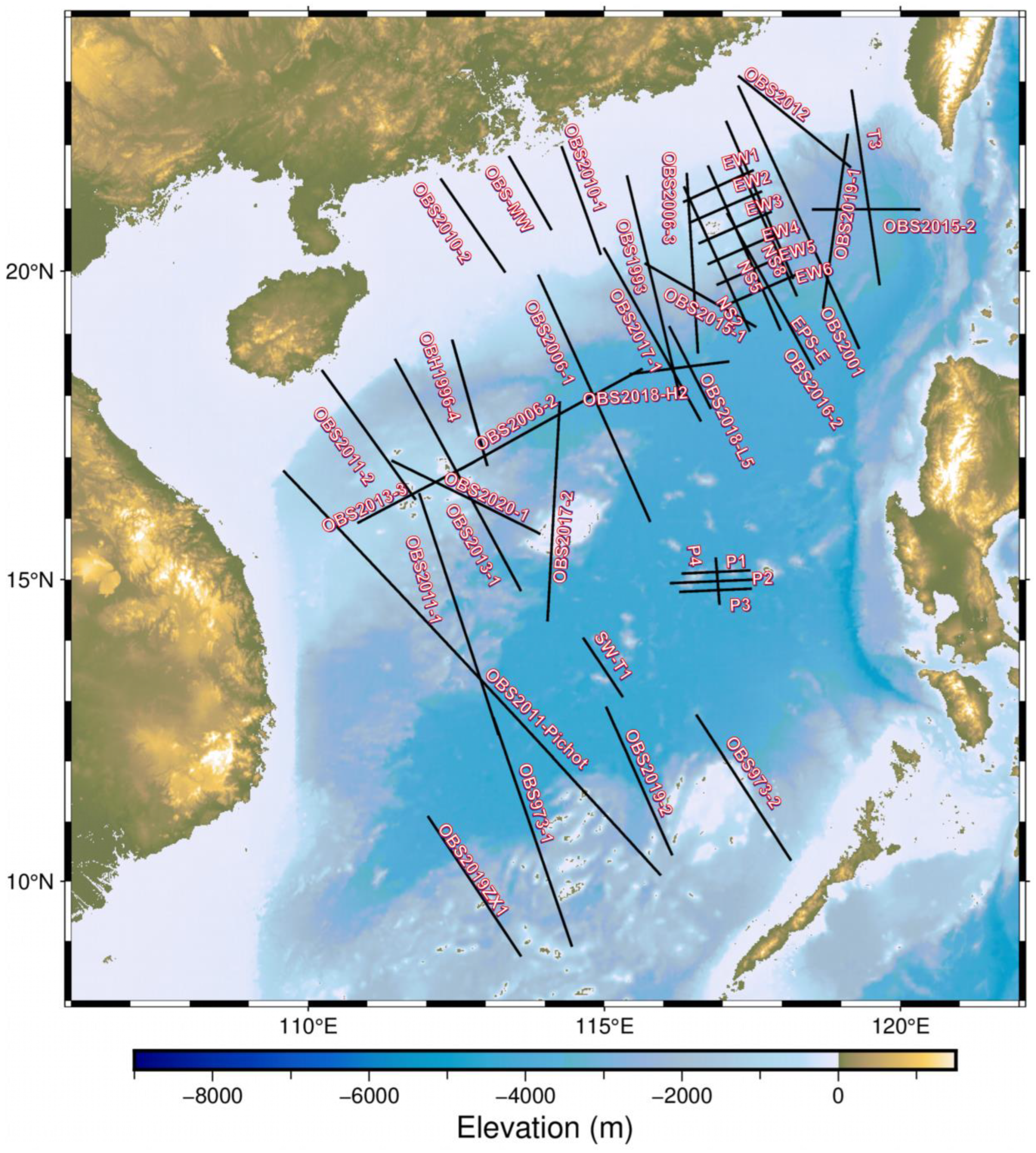
Figure 1. The distribution of the 44 crustal structure profiles in the SCS.
Jmse 12 01907 g001
Figure 2. The auxiliary modeling datasets that were used in this study. (a) IGPP Global Free Air Gravity Anomaly Data_01m. (b) EMAG2 Global Magnetic Anomaly Model_02m. (c) Moho Discontinuity Model. (d) SRTM+ Global Topography Data_01m.
Jmse 12 01907 g002
Figure 3. Algorithm flowchart.
Jmse 12 01907 g003
Figure 4. Network Architecture Diagram.
Jmse 12 01907 g004
Figure 5. Hierarchical modeling strategy.
Jmse 12 01907 g005
Figure 6. (a) The topography, sedimentary layer, upper crust, and lower crust in the modeling results are displayed, along with their corresponding thicknesses of the sedimentary layer (b), upper crust (c), and lower crust (d), respectively.
Jmse 12 01907 g006
Figure 7. The sedimentary interface (a), the crystal crust top interface (b), and the Moho discontinuity (c) in the modeling results.
Jmse 12 01907 g007
Figure 8. The curve graphs depict the variation in the algorithm’s accuracy (a) and training loss (b) with increasing training epochs for a deep artificial neural network simulating geological stratigraphy.
Jmse 12 01907 g008
Figure 9. The curve graph illustrates the variation in training loss and mean absolute error (MAE) with increasing training epochs and iterations, respectively, for a deep artificial neural network simulating the internal velocity structure of the sedimentary layers (a,d), upper crust (b,e), and lower crust (c,f).
Jmse 12 01907 g009
Figure 10. Comparison of 3D P-wave velocity structure models of the SCS constructed by different methods. (ac) Model constructed by the proposed method integrating heterogeneous multi-source data; (df) Model constructed by the proposed method without integrating heterogeneous multi-source data; (gi) Model constructed using Kriging interpolation; (jl) Model constructed using the MPS method.
Jmse 12 01907 g010
Figure 11. OBS2017-2 modeling profile. (a) is the OBS2017-2 profile. (b) Schematic diagram of the location of OBS2017-2 profile data, where the red line represents the OBS2017-2 profile. (c,e,g) are the profiles of OBS2017-2’s position in the model constructed by using multi-source heterogeneous data, not using multi-source heterogeneous data, and Kriging interpolation, respectively. (d,f,h) are the residual maps of these profiles and the OBS2017-2 profile data.
Jmse 12 01907 g011
Figure 12. Comparison of the geologic layer structure thickness (ac), top interface depths (df), and bottom interface depths (gi) displaying the statistics of average, maximum, and minimum values for each layer in the simulation results.
Jmse 12 01907 g012
Figure 13. Comparison of variation function graphs of the simulation results. (ac) represent the statistical results of the depth, east–west, and north–south components, respectively. Due to the different distribution directions of the 44 OBS profiles, the statistical direction of the variation function of the training data in (b,c) corresponds to the direction of the forward profiles.
Jmse 12 01907 g013
Figure 14. Comparison of the simulation results without using the iterative algorithm (a) and the simulation result after using the MPS iterative algorithm (b). The red circles highlight the areas where the artificial artifacts in the model have been corrected after the iteration.
Jmse 12 01907 g014
Figure 15. Cross-sectional views of the crustal structure from the three-dimensional crustal structure model obtained in this study. These sections effectively display the crustal structural characteristics of the northern continental margin, the ocean basin, and the southern continental margin of the SCS, showing good consistency with previous OBS wide-angle seismic research results. A, B, and C show cross-sections extracted from different locations in the three-dimensional crustal structure model.
Jmse 12 01907 g015
Disclaimer/Publisher’s Note: The statements, opinions and data contained in all publications are solely those of the individual author(s) and contributor(s) and not of MDPI and/or the editor(s). MDPI and/or the editor(s) disclaim responsibility for any injury to people or property resulting from any ideas, methods, instructions or products referred to in the content.