Study of Hydrofoil Boundary Layer Prediction with Two Correlation-Based Transition Models

Abstract

In the realm of marine science and engineering, hydrofoils play a pivotal role in the efficiency and performance of marine turbines and water-jet pumps. In this investigation, the boundary layer characteristics of an NACA0009 hydrofoil with a blunt trailing edge are focused on. The effectiveness of both the two-equation gamma theta (γ-Re_θt) transition model and the one-equation intermittency (γ) transition model in forecasting boundary layer behavior is evaluated. When considering natural transition, these two models outperform the shear stress transport two-equation (SST k-ω) turbulence model, notably enhancing the accuracy of predicting boundary layer flow distribution for chord-length Reynolds numbers (Re_L) below 1.6 × 10⁶. However, as Re_L increases, both transition models deviate from experimental values, particularly when Re_L is greater than 2 × 10⁶. The results indicate that the laminar separation bubble (LSB) is sensitive to changes in angles of attack (AOA) and Re_L, with its formation observed at AOA greater than 2°. The dimensions of the LSB, including the initiation and reattachment points, are found to contract as Re_L increases while maintaining a constant AOA. Conversely, an increase in AOA at similar Re_L values leads to a reduced size of the LSB. The findings are essential for the design and performance optimization of water-jet pumps, particularly in predicting and flow separation and transition phenomena.

1. Introduction

Hydrofoils, integral to the design of marine turbines and water-jet pumps, play a pivotal role in the efficiency and performance of these systems [1]. Their design and functionality are crucial for capturing kinetic energy from water flows effectively, translating to better performance and reliability in marine applications [2]. The hydrofoil’s ability to generate lift while minimizing drag is a subject of research, as it directly impacts the overall efficiency of marine vehicles and turbines [3].

In marine engineering, the accurate estimation of boundary layer characteristics on hydrofoils is essential for predicting the internal flow dynamics of water-jet pumps. The boundary layer behavior is particularly important, as it influences the hydrofoil’s interaction with the fluid, affecting lift, drag, and overall propulsion efficiency. The transition from laminar to turbulent flow within this boundary layer is a complex phenomenon that has significant implications for the design and operation of marine systems [4,5].

One of the most prominent characteristics of water-jet pumps is their ability to maintain a very low head while having a substantial flow rate. Consequently, these pumps have garnered extensive use within the energy sector [6,7]. In the research on water-jet pumps, their operational stability has been the focus of attention in engineering applications [8,9]. During the operation of water-jet pumps, a change occurs from laminar to turbulent flow within the boundary layer in the vicinity of the wall. Baltazra [10] and Ye [11] discovered the presence of distinct laminar and turbulent areas in close proximity to the surface of the blade in an experimental study of a water-jet propulsion pump. Boundary layer transition affects the characteristics of blade wall friction, lift/drag ratio, and vortex shedding; therefore, the precise anticipation of boundary layer transition holds significant importance in enhancing the precision of flow prediction within axial pumps. Usually, hydrofoils are used as a simplified model of axial pump blades, and the features hold significant reference value for their design. Guo et al. [12,13] developed a computational model for axial pump gap vortices by studying the cavitation characteristics of the gap vortices of hydrofoils. Wang et al. [14,15] identified a method for the identification of stall vortices of axial pumps by investigating the flow characteristics of hydrofoils’ separating flow method. These studies serve as a valuable resource for examining the internal flow characteristics of axial pumps, specifically focusing on the hydrofoil winding flow; however, there is still a lack of understanding of the transition flow near the vane of axial pumps, and this paper studies the transition characteristics of hydrofoil flow to offer theoretical backing for enhancing the precision of predicting the internal flow characteristics of axial pumps and other similar internal flow systems.

Hydrofoil boundary layer transition was first observed in an experiment. Through experimental observations and measurements, researchers have obtained key parameters and properties of hydrofoil boundary layer transition [16,17]. Examples include the statistical features of turbulence and flow instability and the boundary layer velocity profile. Some scholars have investigated hydrofoil boundary layer stability, obtained the initiation mechanism of transition, and revealed that the emergence of disruptions and the precise site of transition may be accurately anticipated through the utilization of linear stability theory and numerical simulation [18,19]. Researchers have also conducted in-depth studies on the diffusion and growth mechanisms of disturbances, revealing the process of turbulence development, including the formation and expansion of turbulent structures within the boundary layer [20,21]. Researchers have explored a number of control methods to retard or inhibit the transition process in hydrofoil boundary layers. These include methods such as surface texturing [22,23], coatings [24,25], and active control [26,27] to minimize the adverse effects of boundary layer transition on hydrofoil performance.

With the increase in computational power, numerical simulation and optimization algorithms have significantly contributed to the examination of boundary layer transition in hydrodynamic machinery. Investigation into the attributes of a water-jet propulsion axial pump revealed that the incorporation of a transition model enhances the precision of predicting external characteristics [28,29]. This improvement is evident in the reduced discrepancy between the experimental values and the predicted values for both the pressure distribution and the coefficient of friction distribution on the blade surface. Bhattacharyya [30] found that transition models properly portray the transition from laminar to turbulent flow within the context of investigating marine ducted flow. Pawar [31] also studied the transition flow on propellers by adopting the same computational strategy, and the conclusions obtained also verified the importance of considering transition.

Currently, the commonly used transition models are based on the algebraic function intermittent factor model. Among them, Menter proposed the γ and the γ-Re_θt transition models successively in 2006 [32] and 2015 [33]. The γ transition model introduces γ, which represents the local probability of turbulence. The γ-Re_θt transition model combines the γ transition model with the Re_θt approach, in which Re_θt denotes the location within the boundary layer where the transition first starts occurring. The implementation of the γ transition model is somewhat less complex in comparison to the Re_θt approach. It involves solving the regular Navier–Stokes equations as well as an extra transport equation for γ. The γ-Re_θt transition model involves solving both the γ transport equation and the Re_θt transport equation, making it computationally more demanding. Both models have been applied in various flow configurations and engineering applications, such as in aerodynamic design optimization [34,35,36,37] or turbomachinery analysis [38,39,40]. The γ transition model is computationally efficient [41] and the γ-Re_θt transition model is easy to correct. For example, Rubino [42] used a new correlation function to directly establish the relationship between the length parameter of the transition region, the critical momentum Reynolds number and the local flow field, and corrected the shear stress transport (SST) γ-Re_θt transition model, which numerically assesses the accuracy of hydrofoil calculations. The incorporation of Reynolds number and Mach number into the correlation function by Venkatachari [43] was aimed at accurately representing the compressibility of hypersonic flow. Choi [44] established a cross-flow correlation function, which enables the γ-Re_θt transition model to foresee the cross-flow change to increase the accuracy of large-curvature hydrofoils. The transition onset position correlation function proposed by Ye [45,46] was applied to the γ-Re_θt transition model and achieved better results.

The γ model is a turbulence model that focuses on the intermittency variable, γ, which measures the proportion of the boundary layer in a turbulent state, ranging from 0 for purely laminar flow to 1 for fully turbulent flow. This allows for a more detailed depiction of the transition process, with values between 0 and 1 indicating mixed flow phases. The model is known for its gradual prediction of transition from laminar to turbulent flow, which is crucial for accurately simulating complex flow scenarios where the change is not abrupt, but a phased process. A key component of the γ model is its explicit transport equation for the intermittency factor, which takes into account local flow conditions such as velocity gradients, Reynolds number, and surface roughness. This equation is crafted to capture the mechanisms that drive the transition, including disturbances and flow instability [47,48].

Despite the advancements in transition modeling exemplified by the γ and γ-Re_θt transition models, there are still several limitations and challenges that are inherent to current research [49,50]. These challenges primarily stem from the complex nature of transition itself, which involves a multitude of factors and mechanisms that are not yet fully understood. One of the primary limitations is the reliance on empirical correlations, which are often derived from specific experimental conditions and may not generalize well to other flow configurations or off-design conditions. As a result, these models can exhibit significant discrepancies under conditions that deviate from those for which they were calibrated. Another significant challenge is the computational expense associated with models like the γ-Re_θt, which require additional transport equations to be solved [51,52]. This can be particularly prohibitive for industrial applications where rapid turnaround times are essential. The models also tend to have difficulty capturing the effects of unsteady disturbances, such as those caused by surface roughness, freestream turbulence, or pressure gradients, which can significantly influence the transition process. Furthermore, while the SST k-ω model has been improved to include transition modeling, it still tends to predict earlier transition compared to experiments, as it may not fully account for the complex physics involved in the natural transition process. Lastly, the application of these models is often limited to two-dimensional or simple geometries due to the computational cost. However, many practical applications involve three-dimensional or more complex geometries where the transition process can be significantly different [53,54].

In this study, we systematically evaluate the effectiveness of two widely used transition models—the γ-Re_θt and γ transition models—in predicting the boundary layer characteristics of an NACA0009 hydrofoil with a blunt trailing edge. The paper is organized as follows. Section 2 provides a detailed description of the transition models and the modifications made to account for the transition effects. Section 3 presents the numerical setup, including the computational domain, meshing, and boundary conditions. Section 4 analyzes the numerical results, comparing the predictions of the two models with experimental data. Finally, Section 5 concludes the study, summarizing the key findings and suggesting directions for future research.

2. Transition Models

The γ-Re_θt and γ transition models are two widely used approaches in computational fluid dynamics to predict the transition from laminar to turbulent flow in boundary layers. These models are important in the study of hydrofoils and their performance, as the transition significantly impacts lift, drag, and overall propulsion efficiency.

2.1. SST k-ω Model

The SST (shear stress transport) k-ω model is a popular turbulence model used in computational fluid dynamics (CFD) for simulating complex flows. It combines the robustness of the k-ω model in the near-wall region with the free-shear layer accuracy of the k-ε model, making it suitable for a wide range of applications, from internal flows to external aerodynamics [55]. The conservation form of the transport equation for turbulent kinetic energy and turbulent specific dissipation rate is:

$${\displaystyle \frac{\partial \rho k}{\partial t}}+{\displaystyle \frac{\partial \left(\rho {\overline{u}}_{j}k\right)}{\partial x_j}}=P_k-D_k+{\displaystyle \frac{\partial }{\partial x_j}}\left(\left(\mu +{\sigma }_{k3}{\mu }_t\right){\displaystyle \frac{\partial k}{\partial x_j}}\right)$$

(1)

$${\displaystyle \frac{\partial \rho \omega }{\partial t}}+{\displaystyle \frac{\partial \left(\rho {\overline{u}}_j\omega \right)}{\partial x_j}}=P_{\omega }-D_{\omega }+{\displaystyle \frac{\partial }{\partial x_j}}\left(\left(\mu +{\sigma }_{\omega 3}{\mu }_t\right){\displaystyle \frac{\partial \omega }{\partial x_j}}\right)+2\rho \left(1-F_1\right){\displaystyle \frac{{\sigma }_{\omega 2}}{\omega }}{\displaystyle \frac{\partial k}{\partial x_j}}{\displaystyle \frac{\partial \omega }{\partial x_j}}$$

(2)

where μ_t is the eddy viscosity coefficient and F₁ is a mixed function with values ranging from 0 to 1, which enables the conversion between the k-ε model and the k-ω model. P_ω is the turbulence specific dissipation rate generation term, expressed as the relationship between the turbulence kinetic energy generation term and the eddy viscosity coefficient. D_ω is the turbulence specific dissipation rate destruction term, which is related to the turbulence specific dissipation rate and can balance the transport equation. P_k is the turbulence energy generation term, and represents the relationship between time-averaged Reynolds stress and time-averaged velocity gradient. D_k is the turbulence energy destruction term, and is related to the turbulence dissipation rate. Their expressions are as follows.

$$P_k={\tau }_{ij}{\displaystyle \frac{\partial {\overline{u}}_i}{\partial x_j}}$$

(3)

$${\tau }_{\mathrm{ij}}={\mu }_t\left({\displaystyle \frac{\partial {\overline{u}}_i}{\partial x_j}}+{\displaystyle \frac{\partial {\overline{u}}_j}{\partial x_i}}\right)-{\displaystyle \frac{2}{3}}\rho k{\delta }_{ij}$$

(4)

$$D_k={\beta }^{*}\rho k\omega$$

(5)

Above, τ_ij is the strain rate tensor and β* = 0.09. Coupling the transition model with the SST k-ω turbulence model involves integrating the intermittency factor into the SST k-ω model’s transport equations. The effective intermittency variable, γ, modulates the turbulence production and dissipation terms, allowing the model to account for the local probability of turbulent flow. This coupling enables the SST k-ω model to transition smoothly from laminar to turbulent flows, providing a more realistic prediction of the flow characteristics near the boundary layer.

2.2. γ-Re_θt Transition Model

The γ-Re_θt transition model is based on the transport equation of the intermittency factor γ, which represents the local probability of turbulence. This model also considers the momentum Reynolds number at the transition onset, Re_θt. Re_θt denotes the distance within the boundary layer where transition first starts occurring. The model involves solving both the γ transport equation and the Re_θt transport equation, making it computationally more demanding. However, it provides a more detailed description of the transition process by coupling the γ with the Reynolds number at the transition onset [32]:

$${\displaystyle \frac{\partial \left(\rho \tilde{R}{e}_{\theta t}\right)}{\partial t}}+{\displaystyle \frac{\partial \left(\rho {\overline{u}}_j\tilde{R}{e}_{\theta t}\right)}{\partial x_j}}=P_{\theta t}+{\displaystyle \frac{\partial }{\partial x_j}}\left[{\sigma }_{\theta t}\left(\mu +{\mu }_t\right){\displaystyle \frac{\partial \tilde{R}{e}_{\theta t}}{\partial x_j}}\right]$$

(6)

$${\displaystyle \frac{\partial \left(\rho \gamma \right)}{\partial t}}+{\displaystyle \frac{\partial \left(\rho {\overline{u}}_j\gamma \right)}{\partial x_j}}=P_{\gamma }-E_{\gamma } + {\displaystyle \frac{\partial }{\partial x_j}}\left[\left(\mu +{\displaystyle \frac{{\mu }_t}{{\sigma }_{\gamma }}}\right){\displaystyle \frac{\partial \gamma }{\partial x_j}}\right]$$

(7)

where σ_θt is a constant of 2.0, used to control the diffusion coefficient, and P_θt is the source term used to control the Reynolds number of transition onset momentum in the transport equation. P_γ is the intermittent factor generation term, E_γ is the intermittent factor disruption term, and σ_γ = 1. To establish flow control, the turbulence model must be acted upon by the γ-Re_θt transition model. The coupling of the two models is accomplished by acting on SST k-ω through effective intermittency variables, and the linked turbulence model transport equation has the following form [32]:

$${\displaystyle \frac{\partial \rho k}{\partial t}}+{\displaystyle \frac{\partial \left(\rho {\overline{u}}_{j}k\right)}{\partial x_j}}={\tilde{P}}_k-{\tilde{D}}_k+{\displaystyle \frac{\partial }{\partial x_j}}\left(\left(\mu +{\sigma }_{k3}{\mu }_t\right){\displaystyle \frac{\partial k}{\partial x_j}}\right)$$

(8)

$${\tilde{P}}_k={\gamma }_{eff}{P}_k,\hspace{1em}{\tilde{D}}_k=\min \left(\max \left({\gamma }_{eff},0.1\right),1.0\right)D_k$$

(9)

$${\displaystyle \frac{\partial \rho \omega }{\partial t}}+{\displaystyle \frac{\partial \left(\rho {\overline{u}}_j\omega \right)}{\partial x_j}}=P_{\omega }-D_{\omega }+{\displaystyle \frac{\partial }{\partial x_j}}\left(\left(\mu +{\sigma }_{\omega 3}{\mu }_t\right){\displaystyle \frac{\partial \omega }{\partial x_j}}\right)+2\rho \left(1-{\tilde{F}}_1\right){\displaystyle \frac{{\sigma }_{\omega 2}}{\omega }}{\displaystyle \frac{\partial k}{\partial x_j}}{\displaystyle \frac{\partial \omega }{\partial x_j}}$$

(10)

$${\tilde{F}}_1=\max \left(F_1,F_3\right),\hspace{1em}{F}_3=e^{-{\left({\displaystyle \frac{R_y}{120}}\right)}^8},\hspace{1em}{R}_y={\displaystyle \frac{\rho y\sqrt{k}}{\mu }}$$

(11)

Above, P_k and D_k are the turbulent kinetic energy generation and destruction terms of the SST k-ω turbulence model, respectively. ${\tilde{F}}_1$ is a modified mixed function. The literature has detailed information regarding the exact parameters of the γ-Re_θt transition model [32]. The γ-Re_θt model has several advantages over other transition models. It provides a more detailed and accurate prediction of the transition process, especially in complex flow scenarios. The model’s ability to account for both the intermittency factor and the Reynolds number at the transition onset allows for a better representation of the physical phenomena. Furthermore, the model has been extensively validated and is known for its robustness and reliability in various engineering applications [56,57].

2.3. γ Transition Model

The γ transition model is a valuable tool in CFD for predicting the transition from laminar to turbulent flow. It is particularly useful in simulations where accurate prediction of boundary layer behavior is critical, such as in the analysis of hydrofoils and their aerodynamic performance. Menter and Smirnov introduced the model of γ transition [33], which originates from the γ-Re_θt transition model. The determination of Re_θc can be achieved through the use of variables within the boundary layer, hence substituting Re_θt transportation equation:

$${\displaystyle \frac{\partial \rho \gamma }{\partial t}}+{\displaystyle \frac{\partial \left(\rho u_{j}k\right)}{\partial x_j}}=P_{\gamma }-E_{\gamma }+{\displaystyle \frac{\partial }{\partial x_j}}\left(\left(\mu +{\displaystyle \frac{{\mu }_t}{{\sigma }_{\gamma }}}\right){\displaystyle \frac{\partial \gamma }{\partial x_j}}\right)$$

(12)

The interplay between the generation term and the destruction term inside the source term serves to regulate the magnitude of the intermittent factor. The following is the definition formula for P_γ and E_γ:

$$P_{\gamma }=F_{length}\rho S\gamma \left(1-\gamma \right)F_{onset}, E_{\gamma }=c_{a2}\rho \mathsf{\Omega }\gamma F_{turb}\left(c_{e2}-1\right)$$

(13)

S is the strain rate magnitude and F_length = 100. Ω is the magnitude of the absolute vorticity rate, c_a2 = 0.06, c_e2 = 50, and Ωγ = 1. The propagation of kinetic energy in turbulent systems can be adjusted by changing the source term. The γ transition model is integrated with the SST k-ω turbulence model. The linked equation is given below.

$${\displaystyle \frac{\partial }{\partial t}}(\rho k)+{\displaystyle \frac{\partial }{\partial x_j}}\left(\rho u_{j}k\right)={\tilde{P}}_k+P_k^{lim}-{\tilde{D}}_k+{\displaystyle \frac{\partial }{\partial x_j}}\left[\left(\mu +{\sigma }_k{\mu }_t\right){\displaystyle \frac{\partial k}{\partial x_j}}\right]$$

(14)

$${\tilde{P}}_k=\gamma P_k, {\tilde{D}}_k=\max (\gamma ,0.1)\cdot D_k, P_k={\mu }_{t}S\mathsf{\Omega }$$

(15)

To prevent exaggerating the turbulence strength in the stagnation zone in the source term, the P_k and D_k terms in the SST k-ω model have been employed. These terms allow for the enhancement of turbulent kinetic energy generation at low turbulence intensities. The literature has detailed information regarding the exact parameters of the γ transition model [33]. In computational fluid dynamic (CFD) simulations, the γ model is often used in conjunction with Reynolds-averaged Navier–Stokes (RANS) models to provide more precise predictions of boundary layer development. It offers enhanced representations of the transitional phase, leading to improved forecasts of flow separation, reattachment, and turbulence production compared to traditional RANS models that may struggle to capture the nuances of the transition region [58,59].

3. NACA0009 Blunt Trailing Edge Hydrofoil—Natural Transition

3.1. Modeling and Meshing

Ausoni [60] conducted an experimental study of the NACA0009’s blunt trailing edge hydrofoil wraparound characteristics and obtained the boundary layer flow field characteristics. In order to avoid extensive water rotation and reduce the degree of turbulence in the incoming flow, a steady flow section was added upstream of the test section. The angle of attack tested was 0°. The hydrofoil had an inlet that was 3L away from its leading edge and an outlet that was 5L away from its trailing edge. The empirical findings demonstrated that as a result of the hydrofoil’s influence, the mean velocity of the streamline direction at each position of the inlet differed from that of the entire section to a certain extent (within 2%), as shown in Figure 1. At diverse Reynolds numbers, the turbulence degree of the inlet section was approximately 1% and the hydrofoil boundary layer had an obvious laminar boundary layer zone while the natural transition process was observed. These experimental data on the flow field can serve as a basis for comparing and evaluating the accuracy of numerical calculations. With the use of this comparison, hydrofoil transition characteristics predicted using several models can be determined. The water used in the experiments had the following chemical and physical properties: temperature T = 25 °C, viscosity μ = 0.8904 × 10⁻³ Pa·s, density ρ = 997 kg/m³, and surface tension 0.0728 N/m.

These conditions were maintained throughout the study to ensure consistency in the results. The turbulence intensity Tu is defined as follows:

$$Tu=100{\displaystyle \frac{\sqrt{2\mathrm{k}/3}}{U}}$$

(16)

The experimental measurement results of reference [60] indicate that the turbulence intensity Tu, near the leading edge of the hydrofoil, is basically the same at different Reynolds numbers. Based on this, in this article’s calculation, 4% is taken, which is consistent with the experiment.

3.2. Verification of Grid Independence

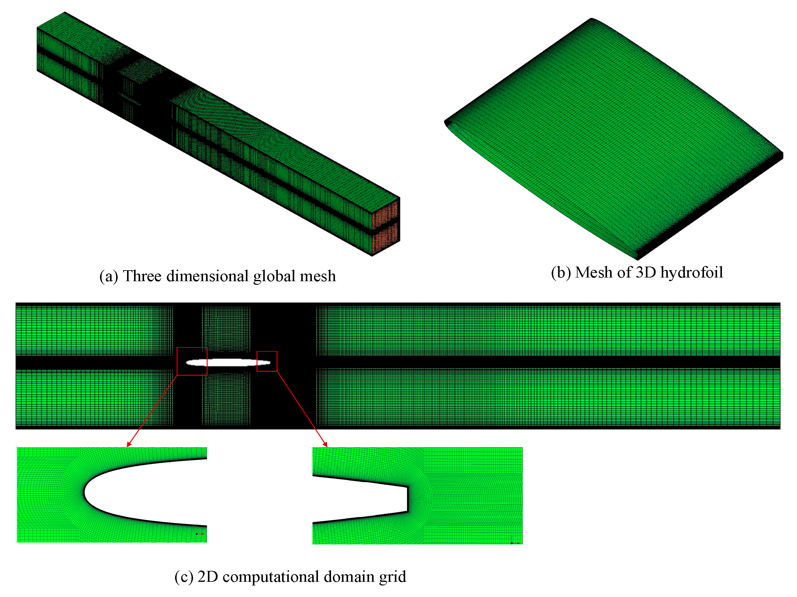
In this study, ICEM CFD 2021R1 software was utilized for mesh generation and preprocessing, playing a crucial role in the accurate resolution of the flow domain around the NACA0009 hydrofoil. The software’s capabilities allow for the creation of a high-quality mesh, which is essential for reliable numerical simulations [61,62]. A study on the applicability of γ-Re_θt grids in airfoil flow field applications was carried out in reference [32]. For hydrofoil wall grids, the grid resolution ranges from 50 ≤ x+ ≤ 150 in the flow direction, 0.77 ≤ y+ ≤ 0.97 in the normal direction of the wall, and 10 ≤ z+ ≤ 40 in the spreading direction. To enhance the quality of a compact boundary layer region in proximity to the wall, O-grids were used. Figure 2 displays the computational domain’s discrete mesh. The implementation of local mesh refinement is carried out in close proximity to the wall to meet the demands of the γ-Re_θt approach, improve the precision of computational calculations, and faithfully depict the critical characteristics of the flow field, with x+_max = 94.6, y+_max = 1.02, and z+_max = 36.4 for the x, y, and z-directions, respectively.

In this paper, a grid-independent study of the γ-Re_θt transition model was carried out. The maximum y+ value of each of the four sets of grids with hydrofoil wall grids is close to 1. Grid M4 is a grid with a relatively large mesh, comprising a total of 2,750,156 individual nodes. Grids M3 and M4 have an equal number of hydrofoil nodes. However, refinements to grid M3 are made not only in the upstream and downstream areas of the hydrofoil but also in the direction perpendicular to the hydrofoil wall, resulting in a node count of 3,885,230. The quantity of surface nodes present on the hydrofoil, including both the leading and trailing edges of the hydrofoil, in grid M2 is twice that of grid M3. There are exactly as many nodes in M1 as there are in M2, except that the quantity of grid nodes along the hydrofoil wall surface is twice that of grid M2. The hydrofoil vortex shedding main frequency is selected as the key parameter, and the vortex shedding main frequency is compared under four sets of grid numbers, as shown in

Table 1. Comparison of wake vortex shedding frequencies with different grid numbers.

Grid	Number of Nodes	Maximum y+	Simulated Value	Tested Value
M1	6,521,238	0.62	1431 Hz	1428 Hz
M2	5,538,952	0.79	1420 Hz
M3	3,885,230	0.93	1336 Hz
M4	2,750,156	1.12	1307 Hz

. The comparison reveals a minimal disparity between grid M1 and grid M2, and the standard errors of the experimental values are within 0.5% considering the computational efficiency, so grid M2 will be used for further calculations.

To precisely assess the flow characteristics of a hydrofoil, it is imperative to employ grid cells of sufficiently tiny size, enabling the precise determination of factors such as boundary layer separation. This research utilized ICEM CFD software to partition the computational domain into hexahedral meshes. Using the finite volume technique, the control equations are discretized on the grids.

The numerical simulations were performed using Ansys Fluent 2021R1, a computational fluid dynamic (CFD) software that employs the finite volume method for solving Navier–Stokes equations. The mixed bounded windward discretization scheme, a term specific to Ansys Fluent, refers to a numerical technique that combines the benefits of first- and second-order discretization schemes. This scheme is used to interpolate the interface values resulting from the discretization of the convective terms, ensuring a balance between accuracy and computational stability. It employs a first-order upwind scheme near the wall, where flow gradients are steep, and a second-order central difference scheme in the outer flow region, where the flow is smoother. This approach helps to accurately capture the flow behavior near the hydrofoil while maintaining solution stability [63,64].

Mixed bounded windward discretization is used to interpolate the interface values that emerge from the discretization of the convection terms while ensuring a maximum level of second-order accuracy. Center-difference interpolation is also used for the interface values that emerge from the discretization of the diffusion terms. For the unsteady Reynolds average simulation (URANS), transient term discretization is implemented utilizing the second-order backward Eulerian scheme, which achieves second-order accuracy. The coupled solution is used for solving the N-S discretized system of equation variables, and a multigrid technique is used to speed up the iterative convergence. The temporal interval between each successive step is 5 × 10⁻⁵ s and the average Courant number is less than 1. The computational aspect described in this context was executed at the High-Performance Computing Center of Eindhoven University of Technology. The computational resources used included 256 GB of RAM and 256 cores, which allows for parallel processing. To investigate the time-varying properties of the shedding vortices, monitoring sites were positioned inside the wake region.

A detailed analysis of the convergence of the two models was conducted. We found that by optimizing the initial conditions and adjusting the physical model parameters, the convergence speed of the models could be improved. We attempted different mesh partitioning strategies to ensure that the mesh was sufficiently refined to capture the spatial changes in the solution field, while avoiding the waste of computational resources caused by excessive mesh partitioning. We added a typical iteration history figure, as shown in Figure 3. In the figure, it can be seen that both models reached convergence after iterating for about 0.05 s of physical time. In addition, we also counted the typical number of iterative cycles required during the simulation process and the order of magnitude of the main residual drop. We found that in most cases, the models required tens of thousands of iterations to reach convergence, and the main residual could drop by as much as six orders of magnitude during the simulation process. This result indicates that although the models have a slower convergence rate, we can still ensure the convergence and accuracy of the models through appropriate adjustments and optimizations.

3.3. Comparative Analysis of 2D and 3D Calculation Results

In this study, the experimental setup involved a blunt trailing edge hydrofoil model tested in a high-speed cavitation tunnel at the EPFL-LMH laboratory [60]. The model was designed to simulate conditions relevant to hydraulic machinery, with a focus on vortex shedding phenomena. The setup included advanced measurement techniques, such as laser Doppler velocimetry (LDV), particle image velocimetry (PIV), and a laser Doppler vibrometer to capture detailed flow field data and hydrofoil vibrations. Data were collected at various free-stream velocities and cavitation indices, with high-precision sensors providing insights into the flow characteristics and structural responses. Analysis of the collected data encompassed time-averaged velocity profiles, vortex shedding frequencies, and vibration amplitudes, employing methods like fast Fourier transform (FFT) for spectral analysis and cross-correlation to assess the coherence and intermittency of the vortex shedding process. This approach allowed for a detailed investigation of the flow dynamics and the influence of cavitation on vortex shedding and hydrofoil vibrations.

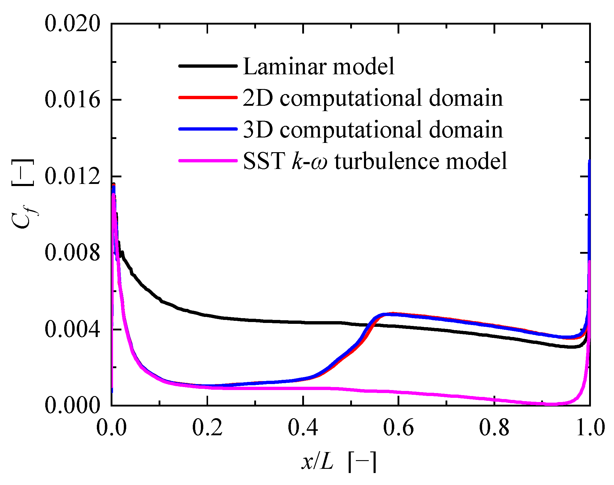
Figure 4 depicts how the wall friction coefficient C_f at the hydrofoil wall distributes under Re_L = 2 × 10⁶. Data from a cross-sectional plane within the 3D computational domain was selected for analysis. The C_f prediction performance of the laminar model is significant within the x/L range, with a maximum value of 0.016, indicating the stress concentration trend of the model under specific conditions. In contrast, although the maximum stress value of the transition model is slightly lower at 0.012, its overall stress distribution is more balanced, indicating that the model can effectively disperse C_f and avoid excessive local C_f when dealing with complex flows. For the 2D computational domain model, the distribution of its calculated values is relatively flat across the entire range, indicating that C_f changes are relatively stable in the 2D computational domain. However, peak stress phenomena were also observed at certain specific x/L values, which may be related to local effects or structural changes in the flow. As for the 3D computational domain model, there is a significant difference in C_f variation trend compared to the 2D model. This difference may be because the 3D domain can better capture the complex structures and phenomena in flow, thereby providing more accurate C_f distribution predictions. However, overall, the stress difference between the 2D and 3D models is not significant.

Figure 5 displays the distribution of H₁₂ of the boundary layer. It is widely accepted that the boundary layer transitions from laminar to turbulent flow as H₁₂ decreases from values greater than 2.6 to less than 1.5, with an intermediate transition state existing between these thresholds [46].

In the hydrofoil leading edge region, the predicted H₁₂ values align closely with experimental data, indicating a reliable result of the flow state. However, after x = 0.2L, the predicted H₁₂ gradually diverges from the experimental values. Notably, the H₁₂ decreases to 1.5 near x = 0.57L, marking the transition to a turbulent state. This is comparable to experimental measurements where the transition occurred at x = 0.85L, which indicates that the transition occurred earlier in the predicted model. Despite these minor differences, there is no significant deviation between the two-dimensional and three-dimensional results. The discrepancies between computational results and experimental data can often be attributed to the limitations inherent in the turbulence models. These models are based on empirical correlations and simplified assumptions that may not fully encapsulate the complex physics of the flow, particularly in regions characterized by high turbulence or near-wall effects.

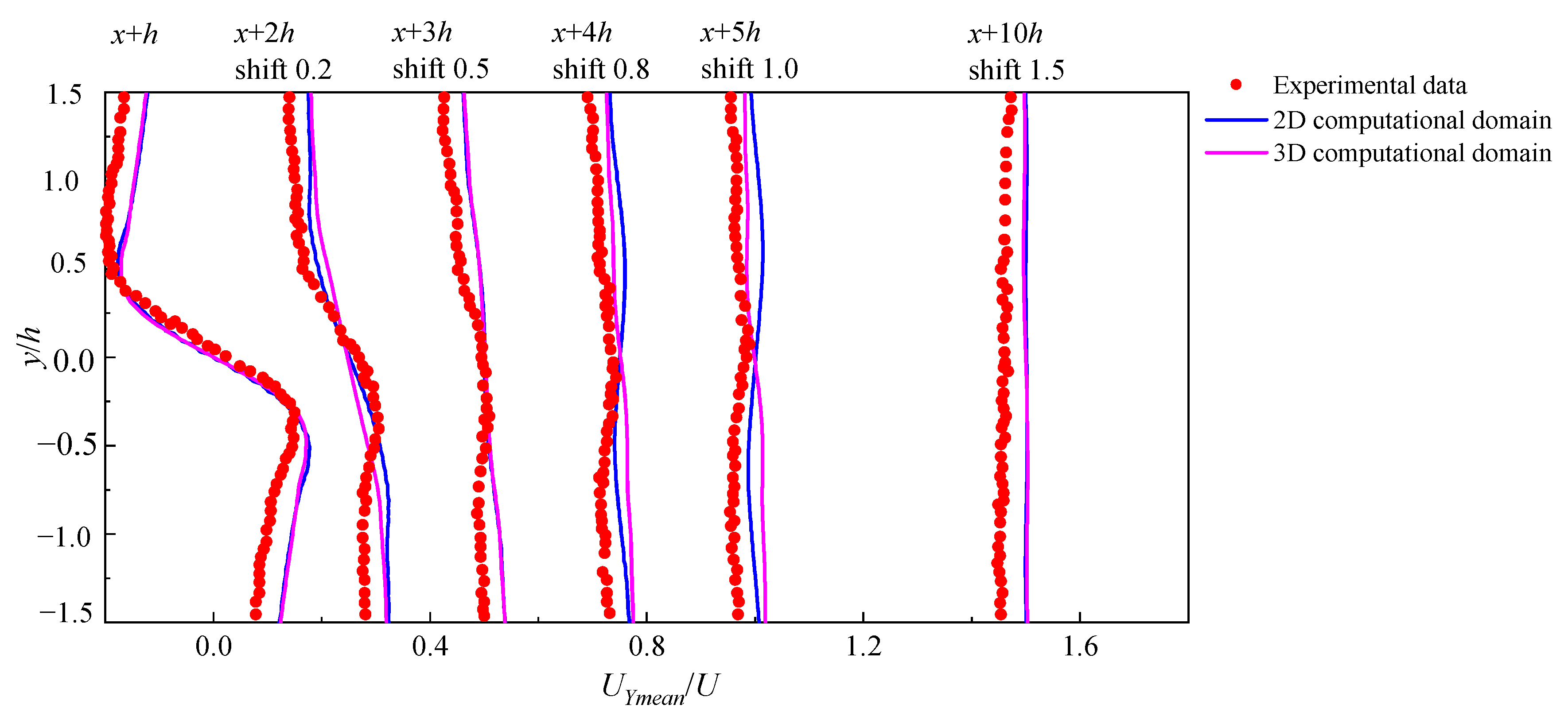
In Figure 6, it can be seen that the disparity between two-dimensional and three-dimensional computations is minimal, with both approaches yielding results that closely align with the experimental values: in the region away from the trailing edge, the three-dimensional calculation closely approximates the experimental value when y takes a positive value, and the two-dimensional calculation closely approximates the experimental value when y takes a negative value, but in general, they all show little difference. To reduce the computational burden, subsequent calculations were carried out using the 2D calculation domain.

3.4. Analysis of Numerical Results

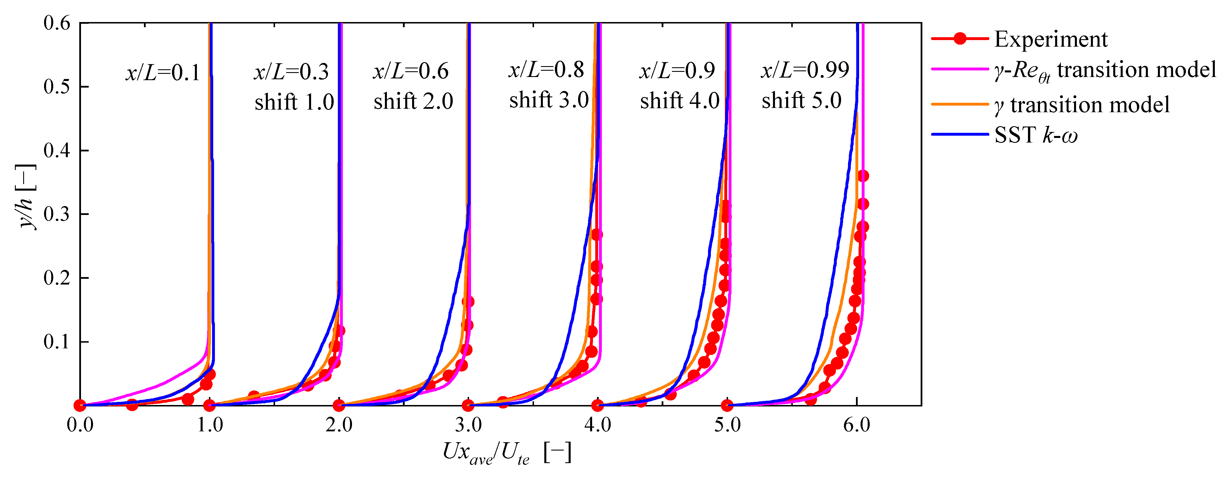
Figure 7 illustrates the results of the hydrofoil boundary layer’s tangential time-averaged velocity distribution, which is calculated by the two kinds of transition models. Within the figure, y designates the distance that is perpendicular to the hydrofoil wall, and h denotes the thickness of the trailing edge. U_xave represents the velocity that is averaged over time at the outermost boundary, and U_te is the time-averaged velocity at the outer edge. The velocity distribution curves for analysis purposes at points x/L = 0.3, 0.6, 0.8, 0.9, and 0.99 are shifted by 1, 2-, 3-, 4-, and 5-unit lengths, respectively, along the horizontal coordinates. Agreement between the velocity distributions of the two models and the experimental data is obtained at the leading edge at a location corresponding to 0.1 times the hydrofoil chord length. However, along the flow direction, velocity distributions calculated by the SST k-ω model show increasing error: the γ transition model is only computed with a larger error close to the aft region of the hydrofoil, i.e., at 0.8 times the hydrofoil chord length.

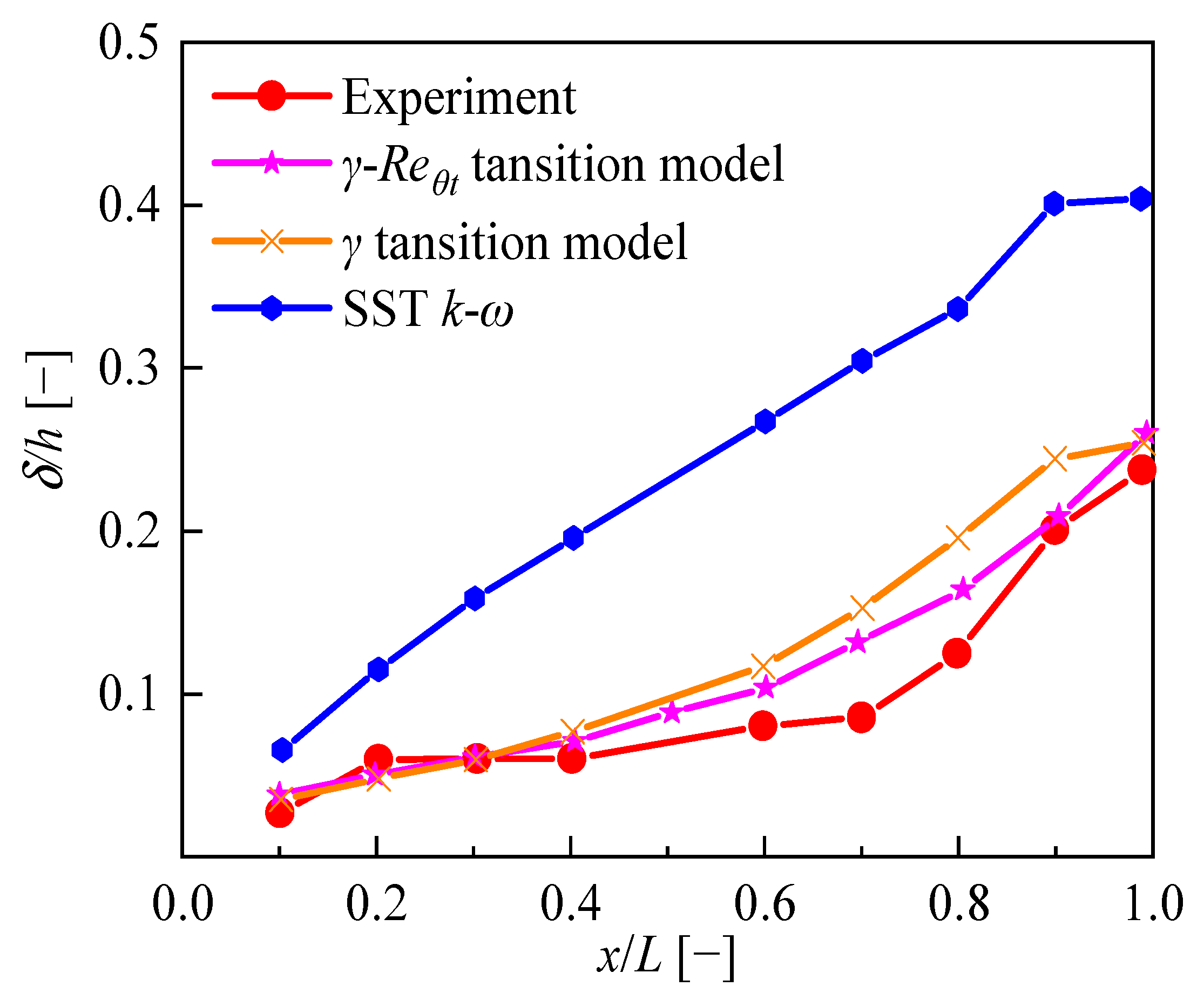
To clarify, the thickness refers to the spatial extent of the hydrofoil boundary layer measured from the adjacent wall (zero velocity) along the normal direction to the position of 0.990 external velocities, denoted as δ, i.e., δ = y|U_x = 99% of U_e. The outcome of the dimensionless thickness δ/h calculated by different models along the hydrofoil chord length is presented in Figure 8. As the boundary layer progresses, the thickness grows with the increasing distance from the leading edge. There exists a substantial disparity in thicknesses computed by these two models. Specifically, the SST k-ω model yields a significantly better thickness compared to the experimental findings. Conversely, thickness at the leading edge, as determined by the γ transition model, exhibits a satisfactory level of concordance with the experimental results.

Figure 9 illustrates the distribution of the shape factor H₁₂ under different models. H₁₂ is a parameter that quantifies the relationship between the displacement thickness δ₁ and its momentum thickness δ₂. When H₁₂ exceeds 2.6, the laminar state is typically observed; when H₁₂ is less than 1.5, the boundary layer is turbulent; and for H₁₂ in the range of 1.5–2.6, it is in a transition state. The shape factor anticipated by the γ transition model deviates from the experimental value after x = 0.2L and decreases to 1.5 near 0.55L, indicating that the transition has been completed at this location, which is earlier than the end of transition observed in the experiment at 0.85L. The γ-Re_θt transition model predicts that the transition endpoint will be close to 0.53L. Although the SST k-ω model has difficulties in capturing laminar flow and transition, while the γ-Re_θt transition model and γ transition model perform better, there are still errors between them and experimental values. This error is particularly evident under high-Reynolds-number conditions, indicating that there is room for further improvement in the model.

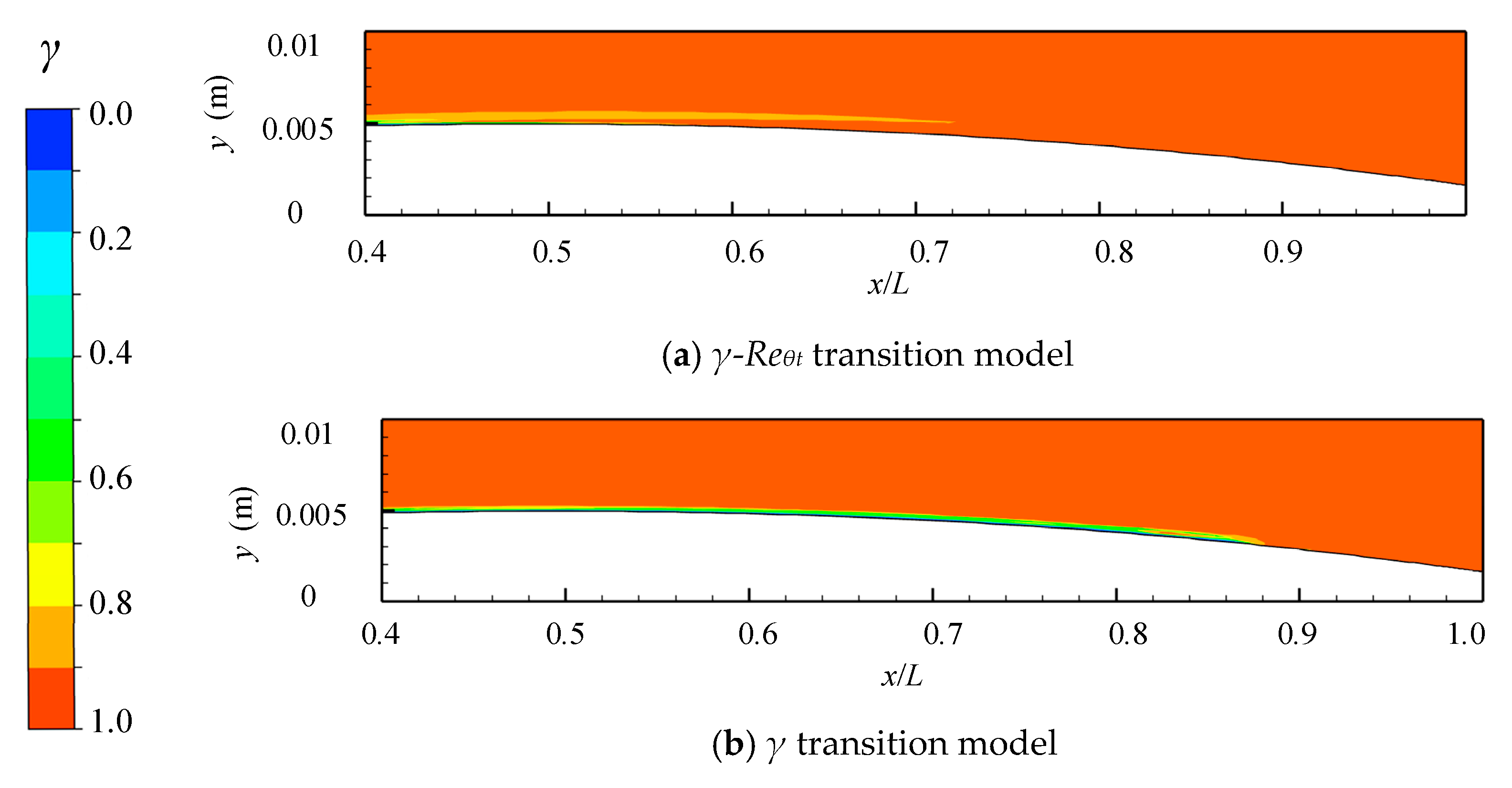
Figure 10 presents the boundary layer intermittency factor distribution obtained using various models for hydrofoil analysis. When employing the SST k-ω turbulence model, the intermittency factor tends to converge towards 1. This observation can be elucidated by the more extensive manifestation of turbulent characteristics beyond the boundary layer under fully turbulent conditions. Conversely, utilizing the γ-Re_θt transition model reveals a rapid increase in the intermittency factor at a distance of 0.4L from the hydrofoil, signifying the onset of transition, and culminating in a transition to a fully turbulent boundary layer at 0.6 chord lengths from the hydrofoil. The γ transition model predicts a gradual rearward shift in the transition location, with the transition end position stabilizing at a distance of 0.9L from the hydrofoil. These findings underscore the efficacy of the γ transition model in accurately predicting the transition position of the hydrofoil boundary layer.

3.5. Prediction Performance Analysis at Different Reynolds Numbers

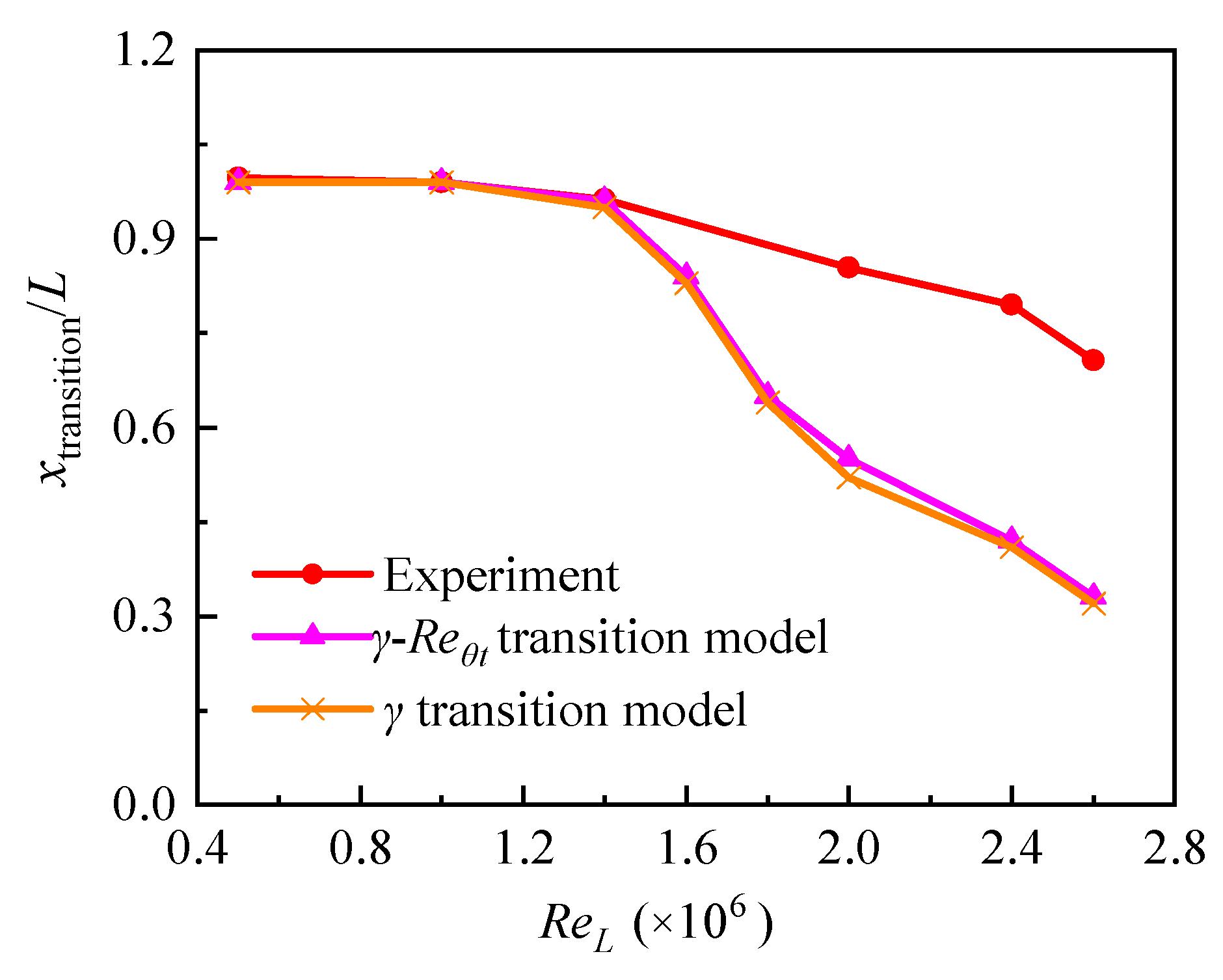
The variation in the full transition site with Reynolds number is depicted in Figure 11, which can be employed to further examine the efficacy of the γ transition model in forecasting the transition of the boundary layer at various Reynolds numbers. Obviously, at a Reynolds number lower than 1.6 × 10⁶, the measured result aligns more consistently with the position, while from Reynolds numbers higher than 1.6 × 10⁶, as the Reynolds number rises, the location of the transition gradually diverges from the measured value. This suggests that the γ transition model is ineffective in accurately predicting boundary layer transition for hydrofoils operating at high Reynolds numbers. According to the relevant literature [65,66], the discrepancies between predicted and experimental values can be attributed to several factors, as suggested by Figure 11. The first is the rapid decrease in turbulence intensity within the free shear layer, especially at high Reynolds numbers. If this is too rapid, an inaccurate estimation of the transition location can result. The second is the necessity of carefully setting a higher turbulence level at the inlet to align with experimental conditions under high-Reynolds-number flows, where an overly high intensity might precipitate an early transition, contradicting experimental observations. Another factor is the potential limitation of the models’ applicability at high Reynolds numbers, where their ability to predict may not fully account for the intricacies of the flow.

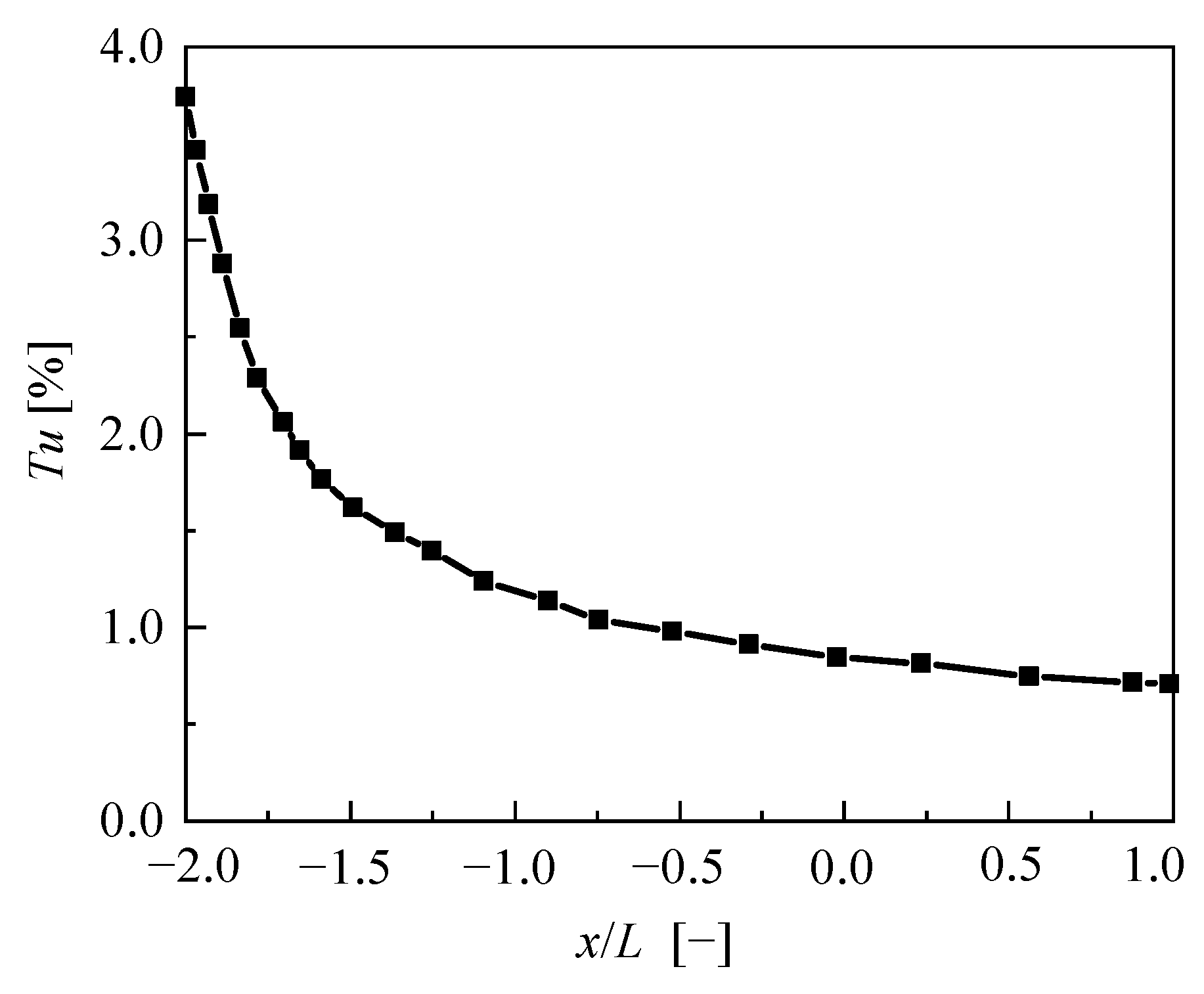
To investigate the causes behind the γ transition model’s poor prediction performance at high Reynolds numbers, the development of turbulence degree Tu along the flow direction is given for a Reynolds number of 2.0 × 10⁶ obtained by numerical calculations shown in Figure 12. It can be seen that the turbulence degree Tu decays rapidly along the flow direction, and the degree of turbulence does not hit 1% when it reaches the leading edge, which is inconsistent with the experimental measurements. Therefore, the inlet of the computational domain at a high Reynolds number must be set to a larger Tu value, but too large a value will accelerate the increase in the predicted value of the intermittency factor γ. This phenomenon results in an accelerated progression of the transition process, and Langtry [32] also pointed out that too large a Tu value will lead to the predicted wall drag coefficient deviating from the laminar flow value. Therefore, the primary cause of the incorrect transition position prediction is the significant degradation of transition in the free-flow field at high Reynolds numbers.

In our current simulation setup, we observed a decay in turbulence intensity within the free stream, which can affect the accuracy of our results, especially at higher Reynolds numbers. To mitigate this decay, future work will explore strategies such as adjusting the free-stream turbulence intensity or employing advanced turbulence models that can better predict and manage turbulence decay. Additionally, we will investigate the impact of different free-stream boundary conditions on the turbulence variables to ensure that they accurately represent the physical flow conditions. Proper management of free-stream turbulence is essential for accurate simulation results, particularly in regions where the boundary layer transitions from laminar to turbulent flow.

4. Analysis of Calculation Results at Different Angles of Attack

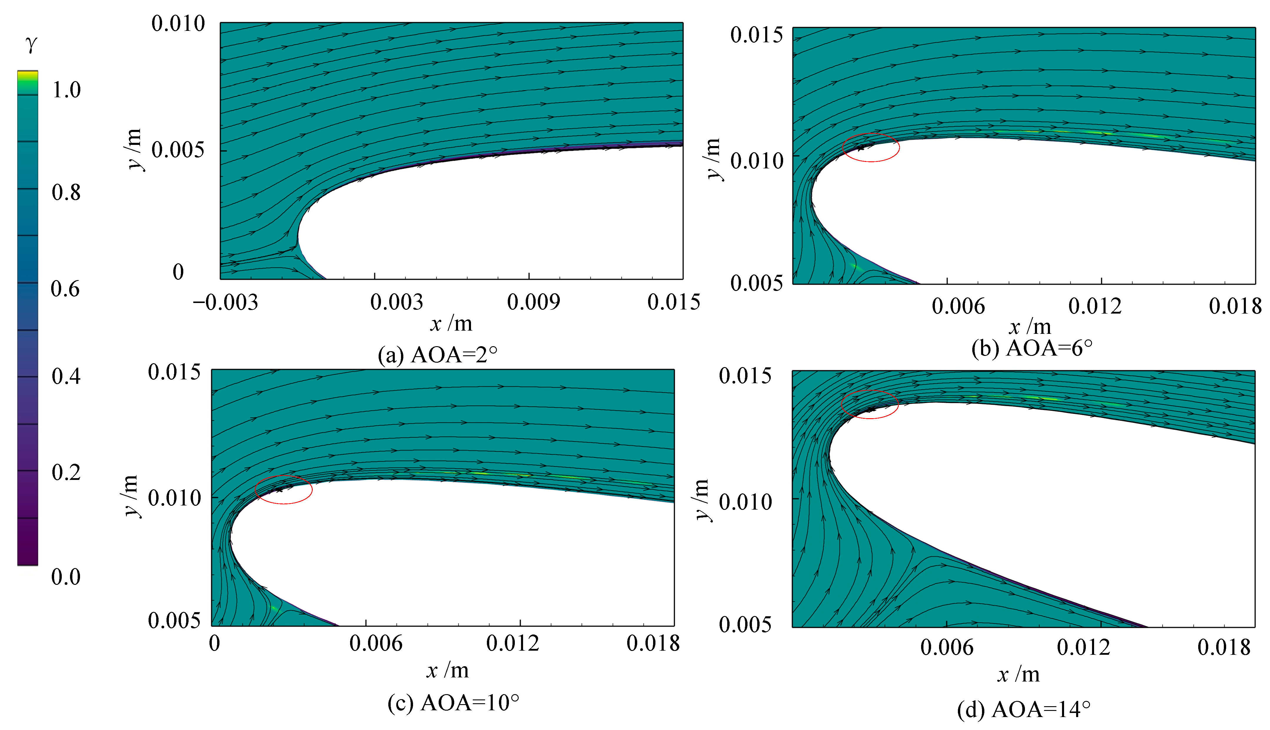
This section uses the γ transition model to study the flow characteristics of hydrofoils, with a focus on analyzing the boundary layer transition characteristics at different angles of attack. Figure 13 shows enlarged boundary layer flow line diagrams of the leading edge at AOA of 2°, 6°, 10°, and 14° under Re_L = 2 × 10⁶, with the cloud reflecting the change in the intermittency factor γ. The laminar separation bubble (LSB) appears in the boundary layer of the leading edge when the AOA is larger than 2° relative to the natural transition at 0°. In the LSB, areas of secondary backward flow and stagnation are present, and the flow downstream of the bubble is turbulent. The laminar separation bubble at 2° extends from x_sep/L = 0.0266 to x_re/L = 0.0622, where x_sep and x_re represent the location of the point of LSB separation and the spot where turbulent flow reattaches, respectively. The relative height is approximately h/L. The h/L of the LSB at 2° is 4.22 × 10⁻⁵. At an AOA of 6°, the LSB spans a range from x_sep/L = 0.0165 to x_re/L = 0.0476, with its height approximating h/L = 4.72 × 10⁻⁵. At an angle of α = 10°, the LSB spans from x_sep/L = 0.017 to x_re/L = 0.029, with a height of approximately h/L = 3.26 × 10⁻⁵. At the location of 0.017L, the boundary layer undergoes a transitional behavior, resulting in the emergence of the LSB. Subsequently, the bubble flow remains attached beyond 0.029L due to the intensified resistance caused by the downstream reverse pressure gradient. Compared with that at α = 10°, when the AOA is increased to 16°, the LSB expands in both the direction of flow and perpendicular to the wall and broadens from x_sep/L = 0.0258 to x_re/L = 0.0374. In fact, an increase in the AOA results in an intensified velocity gradient, causing the vortex to break up into multiple vortices. This guarantees the stability of the separation bubble, with the vortex located upstream being notably diminutive compared to the principal vortex positioned downstream. In a prior study, researchers also identified a twin-eddy arrangement in an airfoil, which was classified as a nonclassical separation bubble [67].

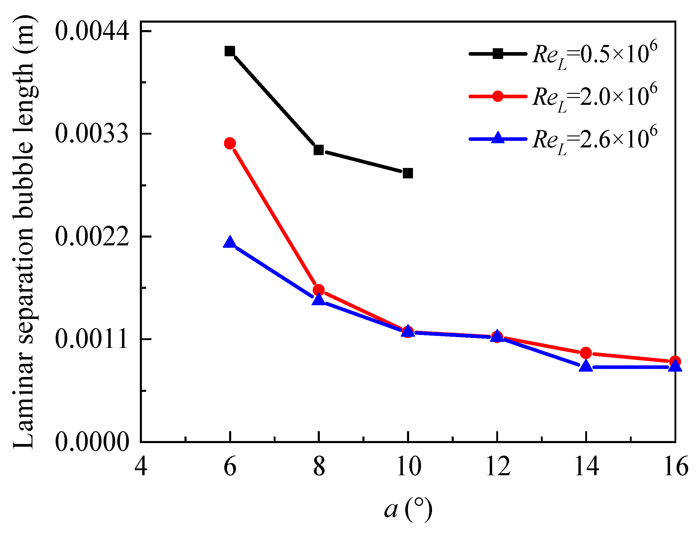
Figure 14 presents a comprehensive depiction of the relationship between the length of the leading edge suction bubble and the AOA across varying Reynolds numbers. As the Reynolds number rises while maintaining a constant AOA, the size of the LSB diminishes. Furthermore, under comparable Reynolds numbers, an increase in the AOA leads to a reduction in the size of the LSB. Notably, both the length and height of the LSB remain relatively stable until the occurrence of trailing edge stall.

Table 2. Location of LSB at three different Re_L values.

	Onset Point (x/L)			Reattachment Point (x/L)
ReL	0.5 × 106	2.0 × 106	2.6 × 106	0.5 × 106	2.0 × 106	2.6 × 106
AOA
6°	0.00164	0.00164	0.00164	0.00578	0.00479	0.00471
8°	0.00147	0.00147	0.00147	0.00456	0.00305	0.00334
10°	0.00102	0.00132	0.00132	0.00385	0.00225	0.00225
12°	/	0.0012	0.0012	/	0.0021	0.00214
14°	/	0.00115	0.00114	/	0.00219	0.00217
16°	/	0.00114	0.00114	/	0.00199	0.00224

shows the variation in the LSB initiation position as well as the turbulence at the reattachment position with AOA for various Reynolds numbers. When Re_L reaches 0.5 × 10⁶ and the angle surpasses 12°, a deep stall ensues, resulting in an inability to record the LSB’s inception point or the turbulence at the point of reattachment. At the same AOA, the LSB initiation location changes rarely. As the Reynolds number rises, the turbulence at the reattachment position shifts upstream along the hydrofoil. With an augmentation in the AOA, the suction surface of the hydrofoil’s leading edge experiences a heightened inverse pressure gradient. This causes the laminar boundary layer to separate earlier, even when the Reynolds number remains constant. Once flow separation occurs at the trailing edge, the LSB’s initiation position and the turbulence at the reattachment location remain largely stationary.

5. Conclusions and Future Prospects

5.1. Conclusions

This study evaluates the accuracy of two transition models in predicting the boundary layer for the NACA0009 blunt trailing edge hydrofoil. The main findings are as follows.

(1)

For natural transition scenarios, the application of the γ-Re_θt and γ transition models significantly improved the predictive capabilities of boundary layer flow distributions in comparison to the SST k-ω turbulence model. At Re_L = 2 × 10⁶, the experimentally determined position for transition completion is 0.85L. In contrast, the SST k-ω turbulence model predicts an earlier transition completion at 0.2L. The γ-Re_θt and γ transition models estimate the transition completion positions at 0.53L and 0.55L, respectively, suggesting a delayed transition relative to the SST k-ω model, but earlier than observed in the experiment.

(2)

For natural transitions, when the Re_L is below 1.6 × 10⁶, the predictive accuracy of both transition models exhibits a notable proximity to the values obtained through experimental analysis. As the Re_L increases, the transition position gradually deviates from the measured value, indicating that the two transition models have poor prediction performance for high-Reynolds-number hydrofoil boundary layer transitions. By analyzing the development of turbulence along the flow direction, it is found that the primary cause of erroneous prediction of transition positions is the significant decrease in turbulence intensity in the free-flow field at high Reynolds numbers.

(3)

Using the γ transition model to study the effects of different angles of attack and Reynolds numbers on the hydrofoil’s leading edge boundary layer, it was found that the occurrence of the LSB is significantly correlated with the AOA, and its size decreases with an increase in the AOA. As the Reynolds number increases, the size of the LSB reduces and remains relatively stable until the onset of the trailing edge stall. Furthermore, an increase in the AOA leads to earlier separation of the boundary layer, which in turn affects the characteristics at the initiation and reattachment points of the LSB.

5.2. Future Prospects

The γ-Re_θt model, with its ability to predict transition points accurately, is set to play a significant role in future studies. Its enhanced predictive capabilities can lead to more efficient designs in aerospace, renewable energy, and naval architecture. Future research could focus on refining the model to handle more complex flow scenarios, such as those involving plasma interactions or bio-inspired surfaces that affect flow transition.

The γ model’s strength lies in its simplicity and effectiveness in predicting transitional flows. Future work could explore the integration of the γ model with advanced numerical methods or machine learning techniques to improve its predictive accuracy further. Additionally, research could be directed towards expanding its applicability to a wider range of Reynolds numbers and flow conditions.

To address the decay of turbulence in the free stream, which is a common issue in many CFD simulations, future studies could explore the following approaches: investigate the potential of the SST k-ω model in sustaining turbulence levels in the free stream—this model could be tested against a variety of experimental data to assess its effectiveness; explore methods of managing turbulence decay by adjusting the free-stream turbulence values—this could involve setting the turbulence values to minimal levels that ensure the desired free-stream turbulence level without excessive decay; and develop or refine advanced turbulence models that can better predict and manage the decay of turbulence, leading to more accurate CFD simulations.

References

1. Zhao, D.; Zhang, Y.; He, Q.; Sun, C.; Bi, M. Hydrodynamic and flow field characteristics of water jet propulsion under mooring conditions. J. Mar. Sci. Eng. 2022, 10, 953. [Google Scholar] [CrossRef]
2. Shi, Z.; Tan, X.; Wang, Y.; Lv, P.; Zou, Y.; Wan, X.; Lv, K.; Li, B.; Duan, H.; Li, H. Experimental Investigation of High Speed Cross-Domain Vehicles with Hydrofoil. J. Mar. Sci. Eng. 2023, 11, 152. [Google Scholar] [CrossRef]
3. Sheha, A.A.A.; Engineer, P.P.C.R.E.; Nasr, M.; Hosien, M.A.; Wahba, E. Computational and experimental study on the water-jet pump performance. J. Appl. Fluid Mech. 2018, 11, 1013–1020. [Google Scholar] [CrossRef]
4. Gupta, S.; Sharma, A.; Agrawal, A.; Thompson, M.C.; Hourigan, K. Role of Shape and Kinematics in the Hydrodynamics of a Fish-like Oscillating Hydrofoil. J. Mar. Sci. Eng. 2023, 11, 1923. [Google Scholar] [CrossRef]
5. Ye, C.; Zheng, Y.; Kan, K.; Tao, R.; Chen, H. Advances in Hydrodynamics of Water Pump Station System. Water 2024, 16, 1430. [Google Scholar] [CrossRef]
6. Kan, K.; Chen, H.; Zheng, Y.; Zhou, D.; Binama, M.; Dai, J. Transient characteristics during power-off process in a shaft extension tubular pump by using a suitable numerical model. Renew. Energy 2021, 164, 109–121. [Google Scholar] [CrossRef]
7. Ye, C.; An, D.; Huang, W.; Heng, Y.; Zheng, Y. Investigation on stall characteristics of centrifugal pump with guide vanes. Water 2023, 15, 21. [Google Scholar] [CrossRef]
8. Arabnejad, M.H.; Svennberg, U.; Bensow, R.E. Numerical Assessment of Cavitation Erosion Risk in a Commercial Water-Jet Pump. J. Fluids Eng. 2022, 144, 051201. [Google Scholar] [CrossRef]
9. Qian, Z.; Wang, F.; Guo, Z.; Lu, J. Performance evaluation of an axial-flow pump with adjustable guide vanes in turbine mode. Renew. Energy 2016, 99, 1146–1152. [Google Scholar] [CrossRef]
10. Baltazar, J.; Rijpkema, D.; de Campos, J.F. On the use of the γ-Reθt transition model for the prediction of the propeller performance at model-scale. Ocean. Eng. 2018, 170, 6–19. [Google Scholar] [CrossRef]
11. Ye, C.; Huang, W.; Yan, H.; Zheng, Y.; Kan, K.; van Esch, B.P.M. Study on rotating stall characteristics of centrifugal pumps based on gamma transition model. Phys. Fluids 2024, 36, 055101. [Google Scholar] [CrossRef]
12. Guo, Q.; Huang, X.; Qiu, B. Numerical investigation of the blade tip leakage vortex cavitation in a waterjet pump. Ocean. Eng. 2019, 187, 106170. [Google Scholar] [CrossRef]
13. Guo, Q.; Zhou, L.; Wang, Z. Numerical evaluation of the clearance geometries effect on the flow field and performance of a hydrofoil. Renew. Energy 2016, 99, 390–397. [Google Scholar] [CrossRef]
14. Wang, C.; Wang, F.; Li, C.; Chen, W.; Wang, H.; Lu, L. Investigation on energy conversion instability of pump mode in hydro-pneumatic energy storage system. J. Energy Storage 2022, 53, 105079. [Google Scholar] [CrossRef]
15. Wang, C.; Wang, F.; Xie, L.; Wang, B.; Yao, Z.; Xiao, R. On the vortical characteristics of horn-like vortices in stator corner separation flow in an axial flow pump. J. Fluids Eng. 2021, 143, 061201. [Google Scholar] [CrossRef]
16. Ducoin, A.; Astolfi, J.A.; Deniset, F.; Sigrist, J.-F. Computational and experimental investigation of flow over a transient pitching hydrofoil. Eur. J. Mech. B/Fluids 2009, 28, 728–743. [Google Scholar] [CrossRef]
17. Ducoin, A.; Astolfi, J.A.; Gobert, M.-L. An experimental study of boundary-layer transition induced vibrations on a hydrofoil. J. Fluids Struct. 2012, 32, 37–51. [Google Scholar] [CrossRef]
18. Posa, A.; Broglia, R.; Balaras, E. Flow over a hydrofoil in the wake of a propeller. Comput. Fluids 2020, 213, 104714. [Google Scholar] [CrossRef]
19. Li, X.; Liu, Y.; Zhu, Z.; Lin, P.; Li, L. Boundary vorticity analysis and shedding dynamics of transient cavitation flow around a twisted hydrofoil. J. Fluids Eng. 2021, 143, 071501. [Google Scholar] [CrossRef]
20. Carabineanu, A. The study of the potential flow past a submerged hydrofoil by the complex boundary element method. Eng. Anal. Bound. Elements 2014, 39, 23–35. [Google Scholar] [CrossRef]
21. Kant, R.; Bhattacharyya, A. A bio-inspired twin-protuberance hydrofoil design. Ocean Eng. 2020, 218, 108209. [Google Scholar] [CrossRef]
22. Churkin, S.A.; Pervunin, K.S.; Kravtsova, A.Y.; Markovich, D.M.; Hanjalić, K. Cavitation on NACA0015 hydrofoils with different wall roughness: High-speed visualization of the surface texture effects. J. Vis. 2016, 19, 587–590. [Google Scholar] [CrossRef]
23. Sedlář, M.; Komárek, M.; Šoukal, J.; Volkov, A.V.; Ryzhenkov, A.V.; Druzhinin, A.A.; Grigoriev, S.V.; Kachalin, G.V.; Kalakutskaya, O.V. Experimental and Numerical Studies into the Cavitation Impact of the Hydrofoil Surface with Different Treatments. Therm. Eng. 2022, 69, 418–428. [Google Scholar] [CrossRef]
24. Rastan, M.R.; Foshat, S.; Sekhavat, S. High-reynolds number flow around coated symmetrical hydrofoil: Effect of streamwise slip on drag force and vortex structures. J. Mar. Sci. Technol. 2019, 24, 500–511. [Google Scholar] [CrossRef]
25. Shahsavari, A.; Nejat, A.; Climent, E.; Chini, S.F. Unexpected trends of lift for hydrofoils with superhydrophobic coating. Eur. J. Mech. B/Fluids 2023, 101, 219–226. [Google Scholar] [CrossRef]
26. Ye, C.; Xia, K.; Yan, H.; Cao, S.; Wang, Z.; Tian, Q.; van Esch, B.P.; Zheng, Y.; Yang, C. Study on the influence of volute structure on the performance of seawater-pumped storage hydropower plant unit. J. Energy Storage 2024, 90, 111848. [Google Scholar] [CrossRef]
27. Kundu, P. Numerical simulation of the effects of passive flow control techniques on hydrodynamic performance improvement of the hydrofoil. Ocean Eng. 2020, 202, 107108. [Google Scholar] [CrossRef]
28. Ge, M.; Svennberg, U.; Bensow, R.E. Improved prediction of sheet cavitation inception using bridged transition sensitive turbulence model and cavitation model. J. Mar. Sci. Eng. 2021, 9, 1343. [Google Scholar] [CrossRef]
29. Kan, K.; Yang, Z.; Lyu, P.; Zheng, Y.; Shen, L. Numerical study of turbulent flow past a rotating axial-flow pump based on a level-set immersed boundary method. Renew. Energy 2021, 168, 960–971. [Google Scholar] [CrossRef]
30. Bhattacharyya, A.; Krasilnikov, V.; Steen, S. Scale effects on open water characteristics of a controllable pitch propeller working within different duct designs. Ocean Eng. 2016, 112, 226–242. [Google Scholar] [CrossRef]
31. Pawar, S.; Brizzolara, S. Relevance of transition turbulent model for hydrodynamic characteristics of low Reynolds number propeller. Appl. Ocean Res. 2019, 87, 165–178. [Google Scholar] [CrossRef]
32. Menter, F.R.; Langtry, R.; Völker, S. Transition modelling for general purpose CFD codes. Flow Turbul. Combust. 2006, 77, 277–303. [Google Scholar] [CrossRef]
33. Menter, F.R.; Smirnov, P.E.; Liu, T.; Avancha, R. A one-equation local correlation-based transition model. Flow Turbul. Combust. 2015, 95, 583–619. [Google Scholar] [CrossRef]
34. Rezaeiha, A.; Montazeri, H.; Blocken, B. CFD analysis of dynamic stall on vertical axis wind turbines using Scale-Adaptive Simulation (SAS): Comparison against URANS and hybrid RANS/LES. Energy Convers. Manag. 2019, 196, 1282–1298. [Google Scholar] [CrossRef]
35. Fahland, G.; Stroh, A.; Frohnapfel, B.; Atzori, M.; Vinuesa, R.; Schlatter, P.; Gatti, D. Investigation of blowing and suction for turbulent flow control on airfoils. AIAA J. 2021, 59, 4422–4436. [Google Scholar] [CrossRef]
36. D’amato, E.; Notaro, I.; Piscopo, V.; Scamardella, A. Hydrodynamic design of fixed hydrofoils for planing craft. J. Mar. Sci. Eng. 2023, 11, 246. [Google Scholar] [CrossRef]
37. Rahman, M.M.; Hasan, K.; Pan, H. Capturing transition around low-Reynolds number hydrofoil with zero-equation transition model. Phys. Fluids 2022, 34, 074115. [Google Scholar] [CrossRef]
38. Cui, B.; Wang, X.; Wang, R.; Xiao, Z. Numerical investigation of transonic axial compressor rotor flows using an improved transition-sensitized turbulence model. Phys. Fluids 2021, 33, 035149. [Google Scholar] [CrossRef]
39. Li, H.; Huang, Q.; Pan, G.; Dong, X.; Li, F. An investigation on the flow and vortical structure of a pre-swirl stator pump-jet propulsor in drift. Ocean Eng. 2022, 250, 111061. [Google Scholar] [CrossRef]
40. Rozhdestvensky, K. A simplified mathematical model of pumped hydrofoils. J. Mar. Sci. Eng. 2023, 11, 913. [Google Scholar] [CrossRef]
41. Durbin, P.A. Some recent developments in turbulence closure modeling. Annu. Rev. Fluid Mech. 2018, 50, 77–103. [Google Scholar] [CrossRef]
42. Rubino, G.; Visonneau, M. Improved crossflow transition predictions for the one-equation γ transition model. Comput. Fluids 2022, 245, 105580. [Google Scholar] [CrossRef]
43. Venkatachari, B.S.; Gosin, S.A.; Choudhari, M.M. Implementation and Assessment of Menter’s Galilean-Invariant γ Transition Model in Overflow. In Proceedings of the AIAA Aviation 2023 Forum, San Diego, CA, USA, 12–16 June 2023. [Google Scholar]
44. Choi, J.H.; Kwon, O.J. Recent improvement of a correlation-based transition model for simulating three-dimensional boundary layers. AIAA J. 2017, 55, 2103–2108. [Google Scholar] [CrossRef]
45. Ye, C.; Tang, Y.; An, D.; Wang, F.; Zheng, Y.; van Esch, B. Investigation on stall characteristics of marine centrifugal pump considering transition effect. Ocean Eng. 2023, 280, 114823. [Google Scholar] [CrossRef]
46. Ye, C.-L.; Wang, C.-Y.; Zi, D.; Tang, Y.; van Esch, B.P.M.; Wang, F.-J. Improvement of the SST γ-Reθt transition model for flows along a curved hydrofoil. J. Hydrodyn. 2021, 33, 520–533. [Google Scholar] [CrossRef]
47. Mykhailyshyn, R.; Duchoň, F.; Virgala, I.; Sinčák, P.J.; Fey, A.M. Optimization of outer diameter bernoulli gripper with cylindrical nozzle. Machines 2023, 11, 667. [Google Scholar] [CrossRef]
48. Santos, D.; Rogers, J.; De Rezende, A.; Maldonado, V. Exploring the Performance Boundaries of a Small Reconfigurable Multi-Mission UAV through Multidisciplinary Analysis. Aerospace 2023, 10, 684. [Google Scholar] [CrossRef]
49. Carreño Ruiz, M.; D’ambrosio, D. Validation of the γ-Reθ transition model for airfoils operating in the very low Reynolds number regime. Flow Turbul. Combust. 2022, 109, 279–308. [Google Scholar] [CrossRef]
50. Mishra, R.K.; Dua, H. Phase transition of cosmological model with statistical techniques. Astrophys. Space Sci. 2020, 365, 1–13. [Google Scholar] [CrossRef]
51. Kontou, M.G.; Trompoukis, X.S.; Asouti, V.G.; Giannakoglou, K.C. The continuous adjoint method to the γ− Reθt transition model coupled with the Spalart–Allmaras model for compressible flows. Int. J. Numer. Methods Fluids 2024, 96, 1715–1740. [Google Scholar] [CrossRef]
52. Pascal, L.; Delattre, G.; Deniau, H.; Cliquet, J. Stability-based transition model using transport equations. AIAA J. 2020, 58, 2933–2942. [Google Scholar] [CrossRef]
53. Ji, B.; Zhong, K.; Xiong, Q.; Qiu, P.; Zhang, X.; Wang, L. CFD simulations of aerodynamic characteristics for the three-blade NREL Phase VI wind turbine model. Energy 2022, 249, 123670. [Google Scholar] [CrossRef]
54. Anzalotta, C.; Joshi, K.; Fernandez, E.; Bhattacharya, S. Effect of forcing the tip-gap of a NACA0065 airfoil using plasma actuators: A proof-of-concept study. Aerosp. Sci. Technol. 2020, 107, 106268. [Google Scholar] [CrossRef]
55. Dewan, A.; Tomar, S.S.; Bishnoi, A.K.; Singh, T.P. Computational fluid dynamics and turbulence modelling in various blades of Savonius turbines for wind and hydro energy: Progress and perspectives. Ocean Eng. 2023, 283, 115168. [Google Scholar] [CrossRef]
56. Chegini, S.; Asadbeigi, M.; Ghafoorian, F.; Mehrpooya, M. An investigation into the self-starting of Darrieus-Savonius hybrid wind turbine and performance enhancement through innovative deflectors: A CFD approach. Ocean Eng. 2023, 287, 115910. [Google Scholar] [CrossRef]
57. Celik, Y.; Ma, L.; Ingham, D.; Pourkashanian, M. Aerodynamic investigation of the start-up process of H-type vertical axis wind turbines using CFD. J. Wind. Eng. Ind. Aerodyn. 2020, 204, 104252. [Google Scholar] [CrossRef]
58. Akhter, Z.; Ali, A.R.; Jawahar, H.K.; Omar, F.K.; Elnajjar, E. Performance enhancement of small-scale wind turbine featuring morphing blades. Energy 2023, 278, 127772. [Google Scholar] [CrossRef]
59. Sridhar, S.; Joseph, J.; Radhakrishnan, J. Implementation of tubercles on vertical axis wind turbines (VAWTs): An aerodynamic perspective. Sustain. Energy Technol. Assessments 2022, 52, 102109. [Google Scholar] [CrossRef]
60. Ausoni, P. Turbulent Vortex Shedding from a Blunt Trailing Edge Hydrofoil (No. THESIS). Ph.D. Thesis, EPFL, Lausanne, Switzerland, 2009. [Google Scholar] [CrossRef]
61. Odetti, A.; Altosole, M.; Bruzzone, G.; Caccia, M.; Viviani, M. Design and construction of a modular pump-jet thruster for autonomous surface vehicle operations in extremely shallow water. J. Mar. Sci. Eng. 2019, 7, 222. [Google Scholar] [CrossRef]
62. Yan, H.; Heng, Y.; Zheng, Y.; Tao, R.; Ye, C. Investigation on pressure fluctuation of the impellers of a double-entry two-stage double suction centrifugal pump. Water 2022, 14, 4065. [Google Scholar] [CrossRef]
63. Zhao, H.-R.; Wang, F.-J.; Wang, C.-Y.; Ye, C.-L.; Yao, Z.-F.; Zhong, Q. A modified VLES model for simulation of rotating separation flow in axial flow rotating machinery. J. Hydrodyn. 2022, 34, 570–584. [Google Scholar] [CrossRef]
64. Huang, Y.; Zhao, M.Q.; Liu, H.T. Numerical Simulation of the Gas Phase of Cyclone-separator Sand Trap Based on ICEM CFD and Fluent. Adv. Mater. Res. 2013, 774–776, 321–325. [Google Scholar] [CrossRef]
65. Sharma, R.; Mishra, D.; Brar, L.S. Performance enhancement of a fin and tube heat exchanger with the novel arrangement of curved winglets using a multi-objective optimization approach. Int. Commun. Heat Mass Transf. 2024, 157, 107804. [Google Scholar] [CrossRef]
66. Bulat, P.; Chernyshov, P.; Prodan, N.; Volkov, K. Control of Aerodynamic Characteristics of Thick Airfoils at Low Reynolds Numbers Using Methods of Boundary Layer Control. Fluids 2024, 9, 26. [Google Scholar] [CrossRef]
67. Wang, R.; Xiao, Z. Transition effects on flow characteristics around a static two-dimensional airfoil. Phys. Fluids 2020, 32, 035113. [Google Scholar] [CrossRef]
Figure 1. NACA0009 blunt trailing edge hydrofoil computational domain.
Jmse 12 01965 g001
Figure 2. Grid diagram.
Jmse 12 01965 g002
Figure 3. Iterative convergence diagrams of two models.
Jmse 12 01965 g003
Figure 4. Distribution of wall friction coefficient (ReL = 2 × 10⁶).
Jmse 12 01965 g004
Figure 5. Boundary layer shape factor distribution (ReL = 2 × 10⁶).
Jmse 12 01965 g005
Figure 6. Distribution of y-direction velocities over time in the wake region (ReL = 2 × 10⁶).
Jmse 12 01965 g006
Figure 7. Tangential time-averaged velocity distribution under different turbulence models.
Jmse 12 01965 g007
Figure 8. Distribution of relative thickness δ/h under various models.
Jmse 12 01965 g008
Figure 9. Distribution of the shape factor H12 for the hydrofoil boundary layer for various models.
Jmse 12 01965 g009
Figure 10. Distribution of the intermittent factor γ for the hydrofoil boundary layer.
Jmse 12 01965 g010
Figure 11. Complete transition position of the boundary layer at different Reynolds numbers.
Jmse 12 01965 g011
Figure 12. Turbulence intensity development along the flow direction.
Jmse 12 01965 g012
Figure 13. Layout of LSB on the surface at different AOA.
Jmse 12 01965 g013
Figure 14. Laminar separation bubble length distributions of hydrofoil.
Jmse 12 01965 g014