Numerical Simulation of Ice and Structure Interaction Using Common-Node DEM in LS DYNA

Abstract

In this work, the icebreaking performance of the cone structure was investigated using a new numerical model called the common-node DEM developed within LS DYNA. The icebreaking characteristics of a typical conical jacket platform in the Bohai Sea focusing on the JZ20-2NW single-pile-leg platform was studied and the ice load characteristics of the cone structure and the dynamic response of the jacket platform under various ice conditions was investigated. The findings indicate that ice thickness significantly impacts the icebreaking mechanism of the cone structure. Specifically, both the peak ice load and the peak acceleration of ice-induced vibrations are proportional to the square of the ice thickness. Additionally, the upward trend in positive vibration displacement of the jacket platform becomes more pronounced with increasing ice thickness. While both the acceleration and displacement caused by ice-induced vibrations on the jacket increase with rising ice velocity, this effect is less significant compared to the influence of ice thickness. Importantly, the ice load remains below the yield strength of the conical shell plate, demonstrating that traditional conical shell plate structures possess a margin of strength redundancy.

1. Introduction

The conical structures that have superior ice-breaking capabilities are commonly used in ice-covered waters [1], such as the Kemi-I lighthouse, Confederation Bridge and jacket platforms in the Bohai Sea (e.g., JZ20-2 MUQ). The way sea ice breaks down is closely linked to the shape of these structures. Furthermore, several effective novel ice-breaking methods have been proposed, such as bubble ice-breaking [2] and water jet ice-breaking [3,4]. When sea ice collides with vertical structures, it shatters into small particles because of crushing fractures. In contrast, it tends to break into fragments while interacting with conical structures following flexural fractures [5,6,7,8]. Since the crushing strength of sea ice is approximately 2–5 times greater than its bending strength, structures with a conical shape can significantly decrease ice loads [9,10]. There are two important factors, i.e., the amplitude and the period, that affect the ice loadings on these conical shapes, and both are closely tied to the ice breaking length [11]. For a constant ice velocity, the load period on the cones is proportional to the breaking length [12]. Moreover, the breaking length offers insight into the sea ice fracture mode, which, in turn, influences the amplitude of the ice load. Various methods, such as numerical simulations, theoretical analyses, model tests and in situ observations, can be employed to study the ice load [13].

Research on conical structure ice loads has employed field measurement systems to gather data on ice loads, ice-induced vibrations, and sea ice parameters [14,15,16]. Qu et al. [17] analyzed the correlation between ice load and vibrations through spectral analysis. However, isolating the impact of individual variables on ice loads is challenging due to environmental complexities and testing inaccuracies. Utilizing field measurements from the JZ20-2 MUQ jacket platform in the Bohai Sea, Xu et al. [18] created a scaling test model at the Hamburg Ship Model Basin (HSVA) to investigate factors influencing ice load on cones. Their findings revealed that ice cover leads to plate-shaped fractures with narrow conical structures and wedge-shaped fractures with wider ones. Additionally, Tian et al. [19] conducted model tests in an ice tank, discovering that ice load increases with cone diameter, provided the ratio of cone diameter to ice thickness is under 30.0. Collectively, these studies highlight the significant roles of cone diameter and ice thickness in affecting ice load and failure modes, although the exact quantitative relationship remains undetermined [20].

The sea ice fracture mode and ice loading during interactions with conical structures is influenced by several key factors, including the cone angle, cone diameter, ice velocity and ice thickness [21,22]. In field measurements and ice tank tests, the sea ice breaking process is primarily observed from a macro perspective, making it challenging to measure the nucleation and initiation of the cracks [23]. This highlights the advantages of numerical simulations, which can effectively calculate ice loads, model the damage processes, and analyze crack formation in sea ice. The finite element method (FEM)[24,25], with its basis in continuum theory and established development, is widely recognized for its reliability in solving engineering problems. However, most FEM software is general-purpose, making it difficult to apply directly to the interactions between sea ice and structures. Recently, a coupling method that combines the FEM with the discrete element method (DEM) has been developed. This approach uses 2D and 3D DEM programs to calculate ice loads in many engineering conditions [26,27]. In this methodology, the DEM calculates the interactions between ice fragments, while the FEM assesses the internal forces within individual fragments, allowing for the simulation of their deformation and collisions. Additionally, other methods include meshless methods such as peridynamics (PD) [28,29,30,31], smoothed particle hydrodynamics (SPH) [32], and mesh methods such as the cohesive element method (CZM) [33], and are also employed in sea ice simulations. While these methods can generally provide reasonable estimates of ice loads, further research is needed to improve the physical phenomenon of sea ice deformation and fracture in simulation.

Since the 1980s, the DEM has been utilized in studying sea ice fracture and the dynamics of floe ice. The DEM can effectively simulate both small-scale collisions between floe ice and analyze the formation of ice ridges, crack initiation, and sea ice fracture in offshore engineering at a mesoscale [34]. Recent advancements in research have focused on the interactions between sea ice and structures, such as platforms or ship hulls, using the DEM [5,35,36]. This approach can accurately simulate the failure processes of sea ice and ocean structures while calculating ice loads and pressure distributions. Furthermore, the DEM excels in capturing the irregular distribution characteristics of ice floe shapes and sizes. During sea ice calculations, simulation variables can be validated by replicating ice mechanics tests, including shearing, bending and compression [37]. The integration of GPU parallel technology has significantly enhanced the computational efficiency and scalability of the DEM, broadening its application in sea ice engineering [38]. The aforementioned studies demonstrate that DEMs of various shapes are extensively used to simulate sea ice floes in broken ice fields and unconsolidated ridges. As a result, DEMs have proven to be effective tools for modeling ice loads on offshore structures and for analyzing the breakage characteristics of sea ice.

In this study, a novel common-node discrete element method is employed to simulate the interaction between level ice and a conical structure [39]. This approach integrates the numerical techniques of the DEM and SPH, allowing for the creation of DEM-SPH particles located on the same node. This research focuses on analyzing the breaking phenomenon, ice-induced vibrations and ice loads on the conical structure using the common-node DEM framework. It investigates how ice thickness and ice velocity affect both the ice breaking length and the load on narrow conical structures. The results are validated by comparing them with our experimental findings.

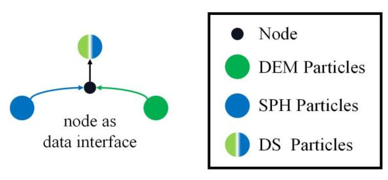
2. The Framework of Common-Node Discrete Element Method

2.1. Basic Principle

Both the DEM and SPH methods gather particle information for calculations, allowing DEM and SPH particles to be established on the same node [39]. This creates a common-node DEM-SPH particle, as illustrated in Figure 1, known as a DEM-SPH particle or DS particle. As a result, a DEM particle can experience forces from other SPH particles at the same node, facilitating fluid–structure interaction (FSI). This combination is referred to as the common-node discrete element–smooth particle hydrodynamic FSI method, or simply the DS-SPH FSI method, also known as the DS method. The examples and modeling techniques utilized in this work are implemented using LS DYNA 2024 R1.

The DS model has the following characteristics: (1) the mechanical properties are primarily governed by DEM particles, with minimal influence from SPH particles; (2) during interactions with the FEM structure, only the DEM particles make contact, while SPH particles do not make contact with the FEM structure. A schematic diagram illustrating the model contact is presented in Figure 2.

The force between DS particles and structures is defined as

$$F_{\mathrm{DS}-\mathrm{FEM}}=SFP\times k_{\mathrm{ni}}\Delta x_{\mathrm{i}}$$

(1)

where SFP represents the contact stiffness, Δx_i denotes the overlap between the i-th particle and the structure, and k_ni is the normal stiffness of the i-th particle, defined as follows:

$$k_{\mathrm{ni}}={\displaystyle \frac{Er}{3(1-2u)}}\times N_{\mathrm{k}}$$

(2)

where E is the elastic modulus of the particle, r is the radius of the particle, v is the Poisson’s ratio, and N_k is the normal stiffness factor of the particles, set to a value of 0.01.

The force acting on the i-th SPH particle arises from both the DS particles and the SPH particles within its support domain, defined as follows:

$$F_{\mathrm{SPH}}=-{\displaystyle \sum _{\mathrm{j}}\frac{m_{\mathrm{j}}\left(p_{\mathrm{i}}+p_{\mathrm{j}}\right)}{2{\rho }_{\mathrm{j}}}}\nabla W\left({\overrightarrow{r}}_{\mathrm{i}}-{\overrightarrow{r}}_{\mathrm{j}},h\right)+\mu {\displaystyle \sum _{\mathrm{j}}{m}_{\mathrm{j}}\frac{{\overrightarrow{u}}_{\mathrm{j}}-{\overrightarrow{u}}_{\mathrm{i}}}{{\rho }_{\mathrm{j}}}{\nabla }^{2}W\left({\overrightarrow{r}}_{\mathrm{i}}-{\overrightarrow{r}}_{\mathrm{j}},h\right)}$$

(3)

where W is the kernel function, p_i and p_j indicate the pressure of i-th and j-th particles, m_j is the mass of SPH particles, h is the smoothing length, ${\overrightarrow{u}}_{\mathrm{i}}-{\overrightarrow{u}}_{\mathrm{j}}$ is the relative velocity, ${\overrightarrow{r}}_{\mathrm{i}}-{\overrightarrow{r}}_{\mathrm{j}}$ is the relative location and ρ_j is the density, defined as follows:

$${\rho }_{\mathrm{j}}={\displaystyle \sum _{\mathrm{i}}{m}_{\mathrm{i}}W\left({\overrightarrow{r}}_{\mathrm{j}}-{\overrightarrow{r}}_{\mathrm{i}},h\right)}$$

(4)

The force on the i-th DS particle is generated by both DS particles and SPH particles within its support domain when the bonding is active, defined as follows:

$$F_{\mathrm{DS}}=-{\displaystyle \sum _{\mathrm{j}}\frac{m_{\mathrm{j}}\left(p_{\mathrm{i}}+p_{\mathrm{j}}\right)}{2{\rho }_{\mathrm{j}}}}\nabla W\left({\overrightarrow{r}}_{\mathrm{i}}-{\overrightarrow{r}}_{\mathrm{j}},h\right)+\mu {\displaystyle \sum _{\mathrm{j}}{m}_{\mathrm{j}}\frac{{\overrightarrow{u}}_{\mathrm{j}}-{\overrightarrow{u}}_{\mathrm{i}}}{{\rho }_{\mathrm{j}}}{\nabla }^{2}W\left({\overrightarrow{r}}_{\mathrm{i}}-{\overrightarrow{r}}_{\mathrm{j}},h\right)}+\left(f_{\mathrm{n}}+f_{\mathrm{s}}\right)$$

(5)

where f_n and f_s represent the normal bonding force and the shear bonding force between the particles, respectively. These are defined as follows:

$$f_{\mathrm{n}}=pb\_k_{\mathrm{n}}\times \Delta u_{\mathrm{n}}$$

(6)

$$f_{\mathrm{s}}=pb\_k_{\mathrm{s}}\times \Delta u_{\mathrm{s}}$$

(7)

where Δu_n and Δu_s denote the normal displacement and shear displacement, respectively; pb_k_n and pb_k_s represent the normal bonding stiffness and shear bonding stiffness, respectively. These are defined as follows:

$$pb\_k_{\mathrm{n}}={\displaystyle \frac{\pi r}{2}}\times pb\_ra{d}^2\times PBN$$

(8)

$$pb\_k_{\mathrm{s}}=pb\_k_{\mathrm{n}}\times PBS$$

(9)

where D is the particle diameter, pb_rad is the bonding factor, PBN is the bonding elastic modulus, and PBS represents the ratio of shear bonding stiffness to normal bonding stiffness, defined as PBS = pb_k_s/pb_k_n.

2.2. Equations of Motion

The force F_i acting on the i-th DS particle is the summation of the forces F_1i and F_2i calculated using SPH. Similarly, the moment M_i is the total moment composed of the moment M_1i computed with the DEM and the moment M_2i from SPH, as described by Newton’s second law:

$$F_i=F_{1i}+F_{2i}=(m_i)\cdot {\ddot{u}}_i$$

(10)

$$M_i=M_{1i}+M_{2i}=I_i{\ddot{\theta }}_i$$

(11)

where ${\ddot{u}}_i$ is the acceleration of the i-th DS particle, m_i represents the total mass of the i-th DS particle, and I_i is the moment of inertia of the i-th DS particle, defined as follows:

$$m_i=(m_{1i}+m_{2i})$$

(12)

$$I_i={\displaystyle \frac{2}{5}}{m}_i{r}_i^2$$

(13)

where m_1i represents the DEM mass of the i-th DS particle, m_2i denotes the SPH mass of the i-th DS particle, and r_i is the DEM radius of the i-th DS particle.

The equation of motion for the particle is solved using the direct integration method. At each time step, the velocity and angular velocity are calculated based on the current acceleration, as well as the angular acceleration, velocity, and angular velocity from the previous time step. The time step is represented by Δt. The formulas are as follows:

$${({\dot{\theta }}_i)}_{n+1}={({\dot{\theta }}_i)}_n+{({\ddot{u}}_i)}_{n+1}\cdot \Delta t$$

(14)

$${({\dot{u}}_i)}_{n+1}={({\dot{u}}_i)}_n+{({\ddot{u}}_i)}_{n+1}\cdot \Delta t$$

(15)

By integrating the particle’s velocity, we can use the velocity, angular velocity, displacement, and angle from the previous time step to determine the current displacement and rotation angle as follows:

$${({\theta }_i)}_{n+1}={({\theta }_i)}_n+{({\dot{\theta }}_i)}_{n+1}\cdot \Delta t$$

(16)

$${(u_i)}_{n+1}={(u_i)}_n+{({\dot{u}}_i)}_{n+1}\cdot \Delta t$$

(17)

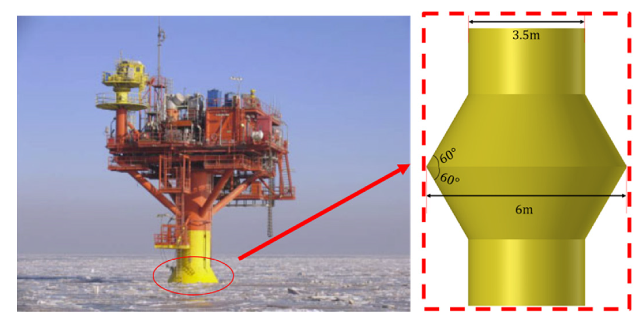
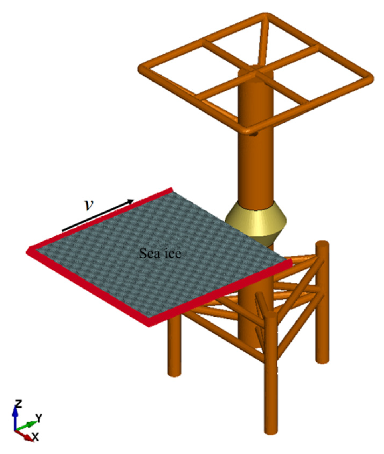
3. Setup of Ice and Structure Simulation

In this work, the JZ20-2NW platform in the Bohai Sea was selected to investigate the inaction of ice and structure, as shown in Figure 3. This platform primarily comprises an upper structure, a jacket, three groups of piles, and a conical structure. The upper structure features a square cross-section with a side length of 12 m and a weight of 250 tons, and it is supported and anchored by the jacket. Each single-leg pile has a diameter of 3.5 m and a total length of 29.5 m, with 13.5 m submerged below the waterline and 16 m extending above it. The three groups of piles are anchored in the seabed, secured by a depth of 6–8 times the diameter of the pile foundation. The conical structure is positioned at the waterline and takes the form of a frustum of a cone, featuring a cone angle of 60° and a maximum diameter of 6 m.

Due to the predominant presence of high-strength large flat ice in the Bohai Sea, flat ice exceeding 30 cm in thickness is seldom encountered in this region, with the maximum ice thickness reaching up to 60 cm. Ice thicker than 40 cm is classified as overlapping ice, with its thickness defined as half that of the measured flat ice thickness. As such, this study focuses exclusively on the interaction between flat ice and structural elements. Figure 4 illustrates the coupling model between the discrete element ice model and the finite element platform. The ice is represented as a square cross-section with a side length of 25 m. The red boundary in the figure indicates the points where boundary conditions for the discrete element ice model are applied. The BOUNDARY_SPC_SET card is utilized to constrain the degrees of freedom in the x and z directions while controlling the ice movement speed in the y direction. The ice speed is defined via the BOUNDARY_PRESCRIBED_MOTION_SET card. To streamline the nonlinear interactions between the pile legs and the seabed, the boundary conditions for the pile legs are represented by an equivalent pile diameter, with the depth of the pile foundation embedded in the seabed set to 6–8 times the pile diameter [40]. This approach rigidly fixes the pile foundation, limiting degrees of freedom in all directions. Both the jacket platform and the conical structure employ shell elements, with a shared node connection at the interface between the cone and the pile legs. The conical structure and the pile legs are constructed using quadrilateral shell elements. The density of the jacket steel is 7850 kg/m³, the Young’s modulus is 210 GPa, and the Poisson’s ratio is 0.3. The mass on the platform is evenly distributed across the corresponding mass points using the ELEMENT_MASS_NODE_SET, while the additional mass of water and air is neglected in the overall model calculation [22]. The conical and jacket structures are combined using the SET_PART_LIST card. To improve the realism of simulating ice-induced vibrations on the jacket platform, it is crucial to account for the friction caused by ice climbing along the cone surface to the pile legs, which contributes to the vibrations in the legs. Consequently, contacts are established between the ice and the cone, pile legs, and overall assembly, defined using the discrete element method contact card DEFINE_DE_TO_SURFACE_COUPLING. The model utilizes an automatic time step setting, with data output intervals of 0.002 s and a total computation time of 20 s. It is recommended to simulate the compression and crushing of level ice with a larger number of particles in the direction of sea ice thickness, such as 3–5 particles. When simulating the bending failure of level ice, fewer particles can be taken in the thickness direction, such as 2–3 particles. In this work, sea ice thickness is set to three particles.

4. Modal Analysis of the Finite Element Model of the JZ20-2NW

Modal analysis is a critical technique for investigating the dynamic characteristics of structures, playing a vital role in understanding and predicting the response of jackets platforms in real-world environments. In the study of the JZ20-2NW platform, modal analysis was conducted on a simplified finite element model to validate its reliability and to delve deeper into the platform’s inherent vibration characteristics. Given that the majority of the jacket platform’s mass is concentrated above the deck, the vibration energy induced by ice loads is primarily concentrated at the fundamental frequency of the structure, with a predominant emphasis on horizontal vibrations. Under the influence of random ice forces, the differential equation of motion governing this finite element model of the jacket platform can be expressed as follows:

$$[M]\left\{\ddot{x}\right\}+[C]\left\{\dot{x}\right\}+[K]\left\{x\right\}=\left\{F\right\}$$

(18)

$$\left\{X\right\}=\left\{x_1{x}_2\dots \dots x_N\right\}$$

(19)

$$\left\{F\right\}={\left\{f_1{f}_2\dots \dots f_N\right\}}^T$$

(20)

where the matrix [M] represents the mass matrix, [C] denotes the damping matrix, and [K] is the stiffness matrix. The vector $\left\{F\right\}$ refers to the external load acting on the structure, while $\left\{X\right\}$ is the displacement vector of the structural nodes. Additionally, $\left\{\ddot{x}\right\}$ represents the acceleration of the structural nodes’ displacement, $\left\{\dot{x}\right\}$ indicates the velocity of the structural nodes’ displacement, and $\left\{x\right\}$ denotes the displacement of the structural nodes. The vibration energy of the structure is mainly concentrated at low-order frequencies of ice loads. In this study, the damping coefficients for 1st, 2nd, 3rd, and 4th orders are taken as 2.0%, 2.1%, 2.2%, 2.3%, and 2.4%, respectively.

For single-pile-leg platforms, the structure is compact, utilizes less steel, and exhibits lower stiffness, which classifies it as a flexible, ice-resistant platform. Its characteristics in response to ice-induced vibrations are relatively simple. In the absence of external forces, the equation of motion for the platform’s free vibrations can be expressed as follows:

$$[M]\left\{\ddot{x}\right\}+[K]\left\{x\right\}=0$$

(21)

In practice, identifying the natural frequencies and mode shapes of a structure is essential for understanding its behavior during free vibrations. Mathematically, this process can be framed as solving the characteristic equation to derive the eigenvalues and eigenvectors. The characteristic equation is generally expressed as follows:

$$K\varphi -{\omega }^{2}M\varphi =0$$

(22)

where $\varphi$ and $\omega$ are the natural frequency and mode of vibration, respectively.

Modal analysis is performed using implicit algorithms, and the CONTRAL_IMPLICIT card is set up to control parameters such as the solution algorithm, control parameters, and characteristic order. The simplified model of the JZ20-2NW platform’s first six natural frequencies and mode shapes is shown in Figure 5.

The simplified platform structure primarily vibrates at its fundamental frequency and mode shapes when subjected to external forces. An analysis of the six modes indicates that the vibrations in the single-leg platform are primarily due to the leg and the upper structure. The calculated natural frequency is 0.754 Hz, which is within the acceptable range for the platform’s natural frequency [41]. Consequently, the simplified model adequately fulfills the analytical requirements for structural dynamic characteristics.

5. Analysis of Simulation Results

In extreme ice conditions, ice-induced vibrations of the jacket platform significantly affect its structural stability and safety. Several factors—such as the speed, thickness, and bending strength of sea ice—contribute to this vibration phenomenon. The formation of sea ice is influenced by natural variables including air temperature, seawater salinity, and brine volume, leading to a certain level of randomness in its thickness and strength. Given the relatively small size span of the single-pile jacket platform conical structure, the sea ice is modeled as square layers with a cross-section of 18 m × 18 m.

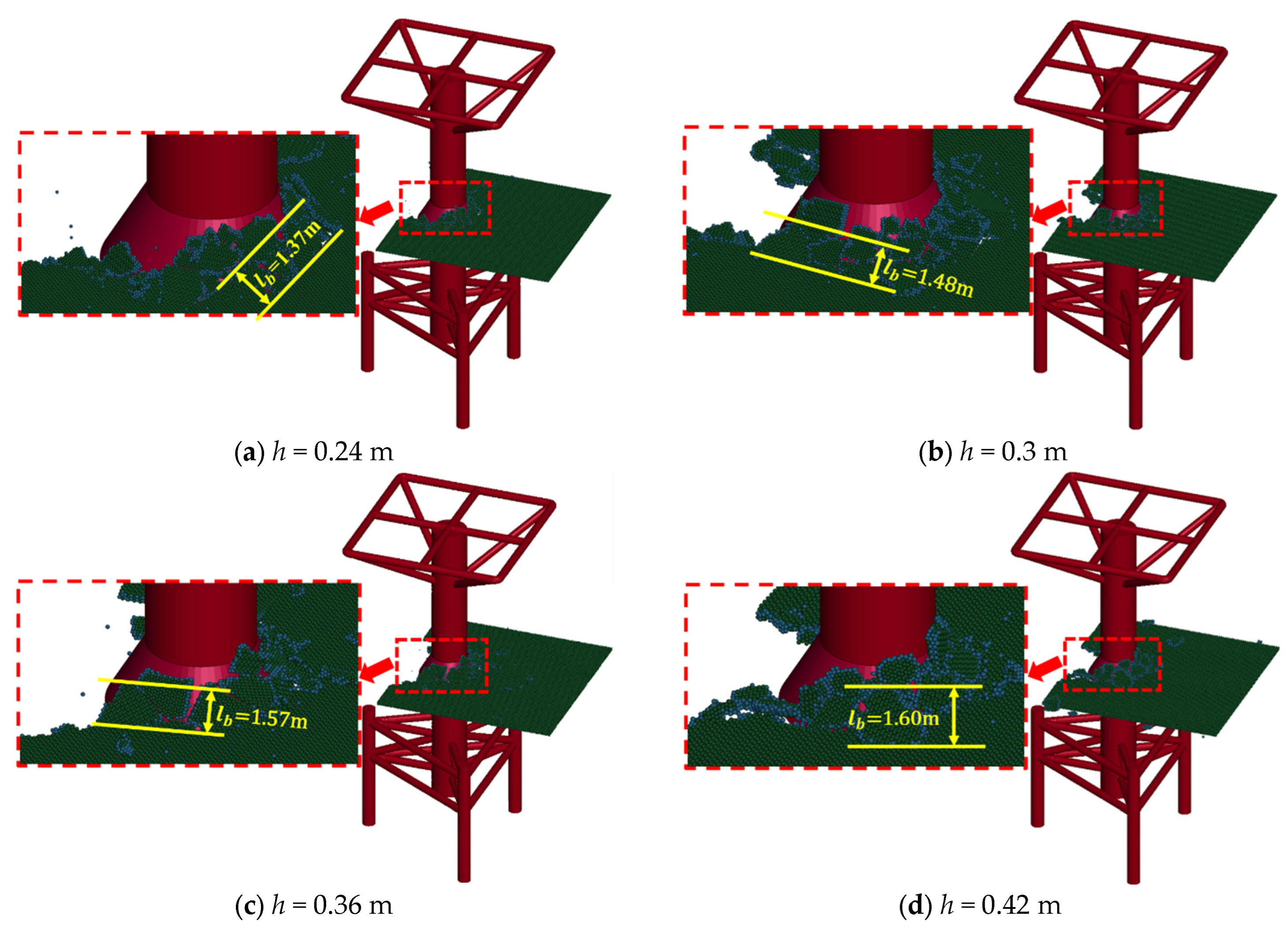
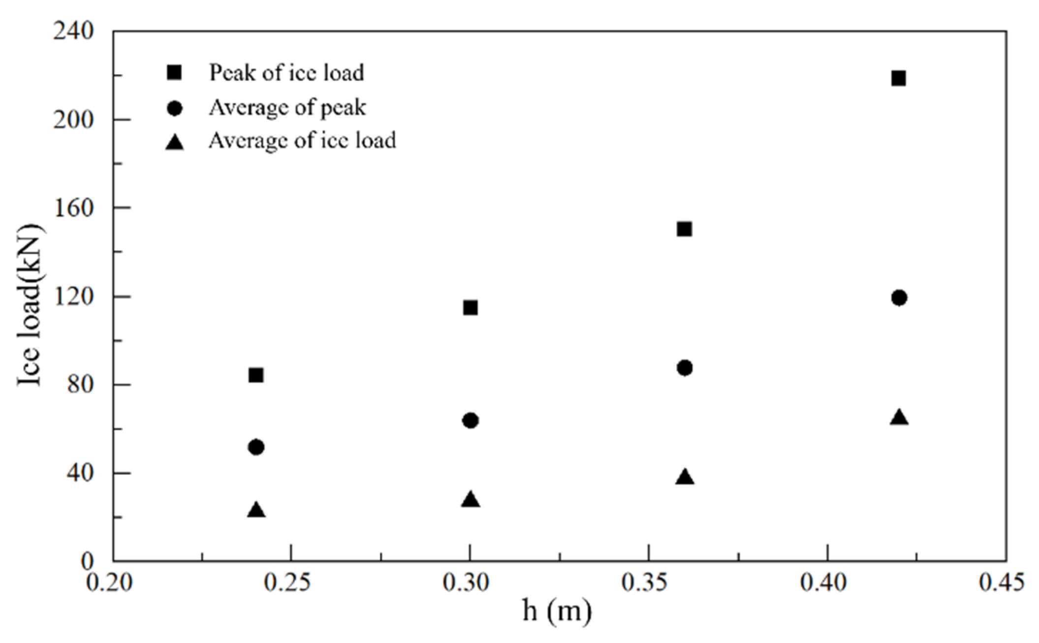
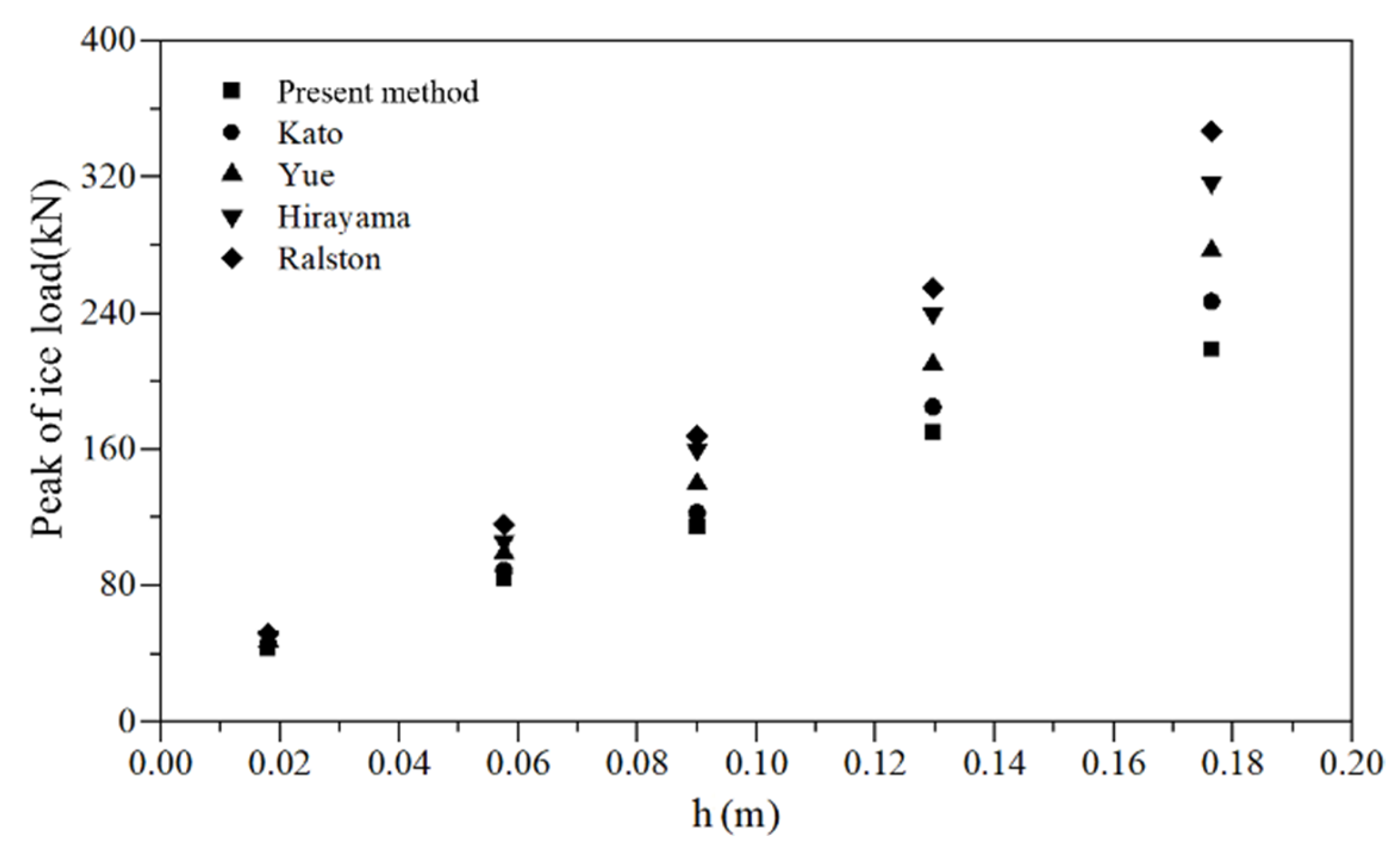
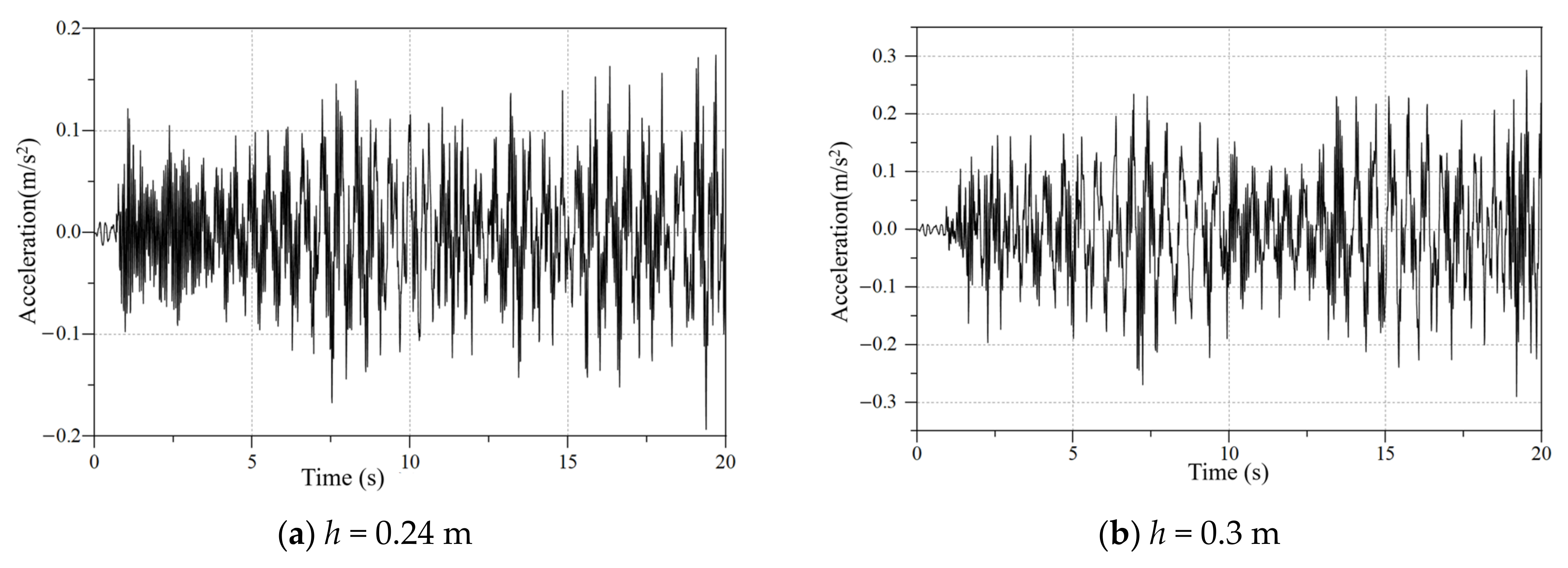
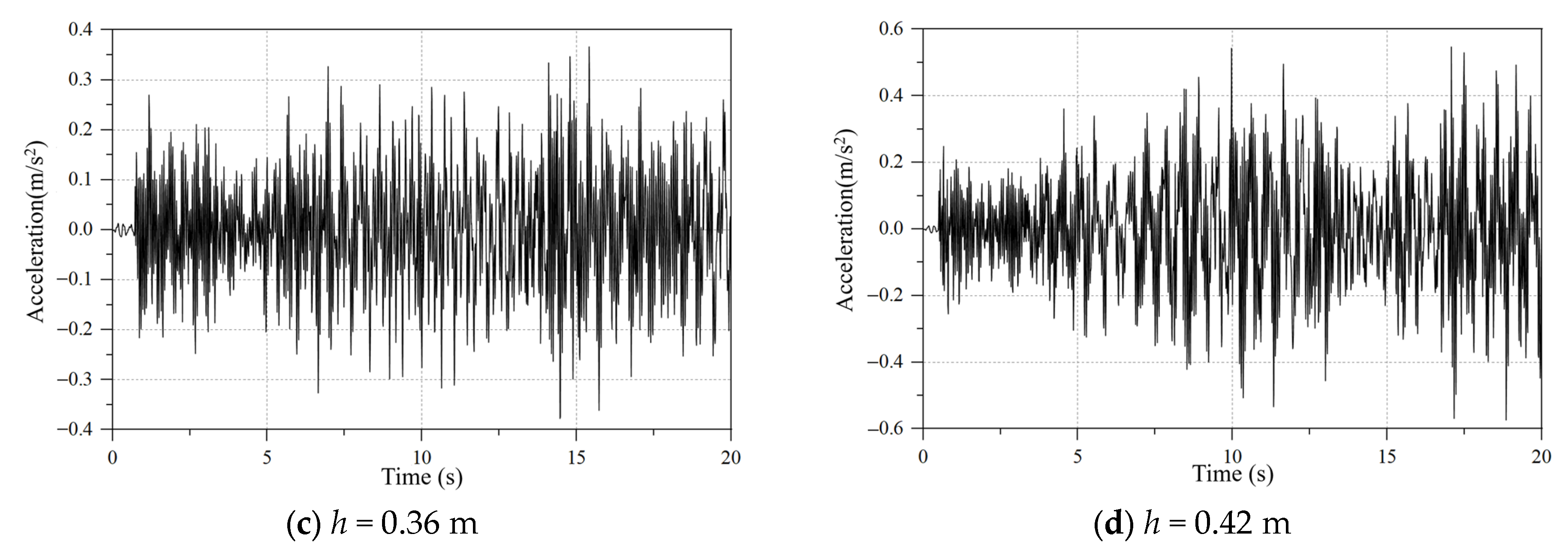
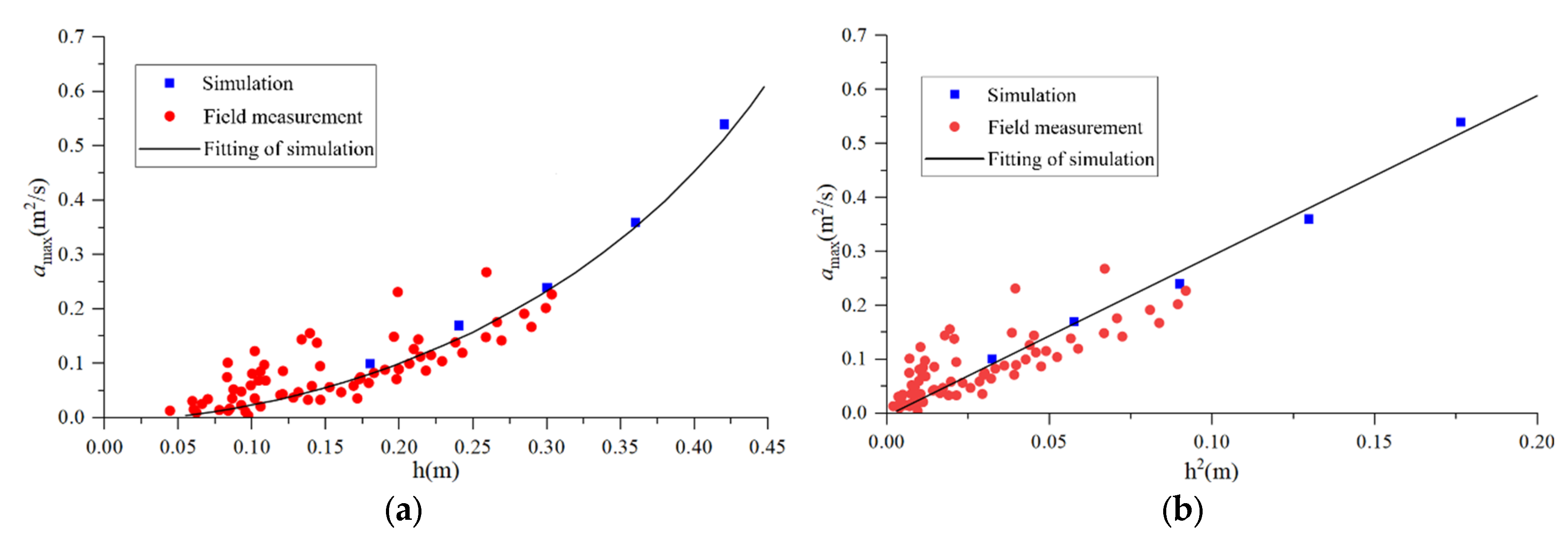
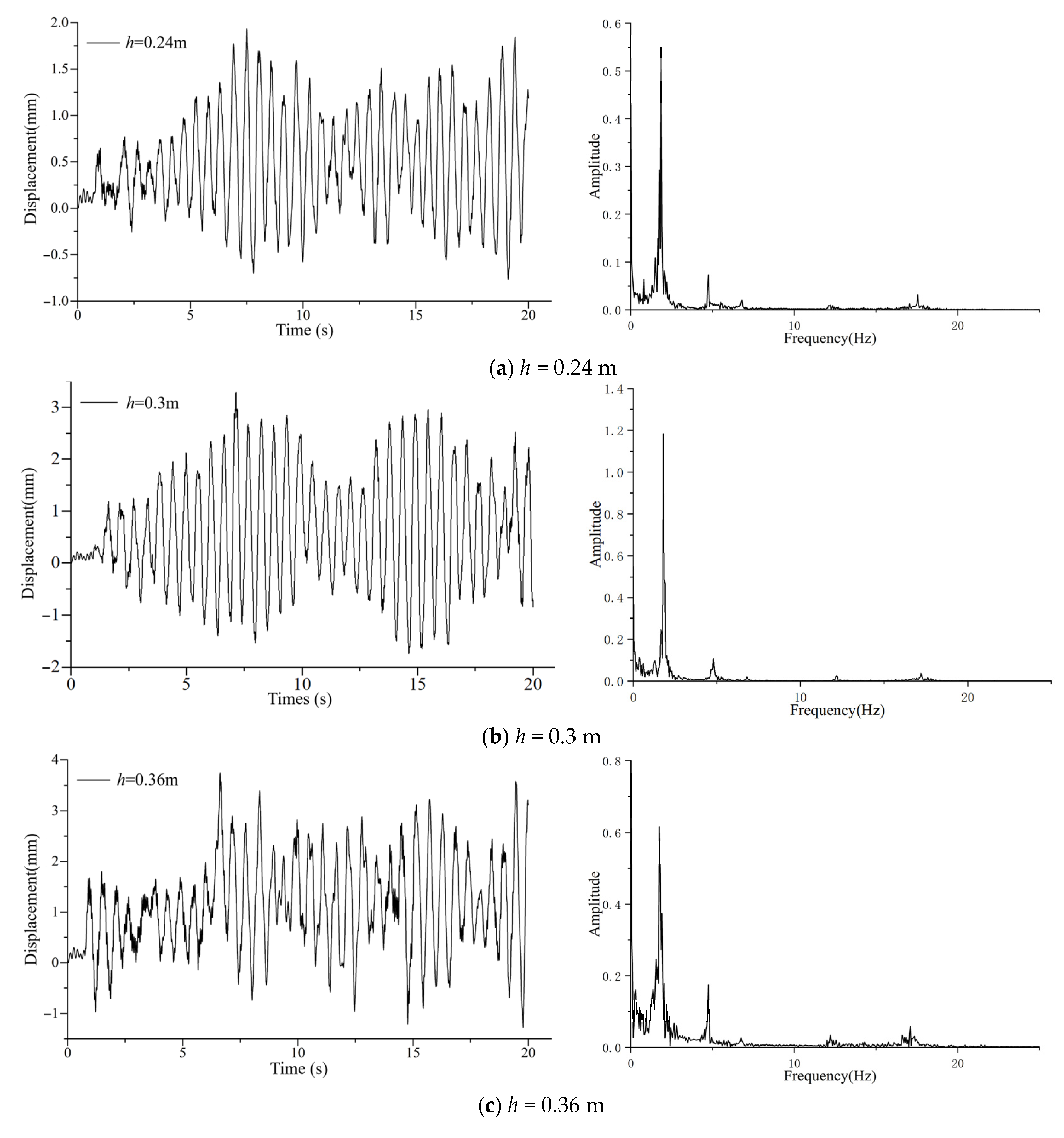
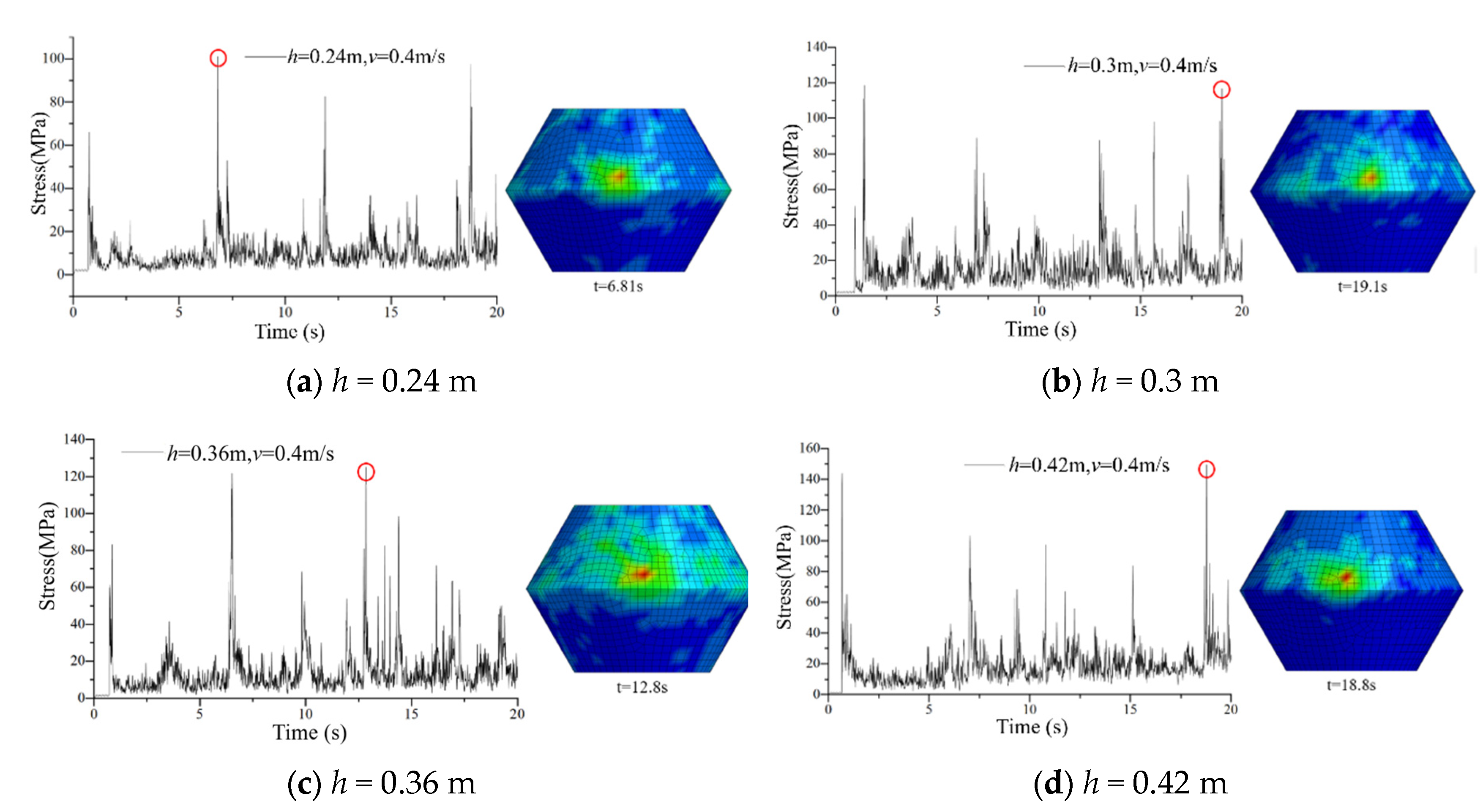
5.1. The Influence of Ice Thickness

For the JZ20-2NW single-pile jacket platform, the dimensions of its conical structure are significantly larger than those of multi-pile jacket structures. Consequently, the influence of ice thickness on ice-induced vibrations requires thorough investigation. The key parameters of the discrete element model for sea ice at varying thicknesses are presented in

Table 1. Parameters related to ice thickness.

Parameter	Value
Sea ice thickness h/m	0.24/0.3/0.36/0.42
Particle diameter D/mm	80/100/120/140
Cementation modulus PBN/MPa	759.1
Ratio of cemented tangential to normal stiffness PBS	0.574
Cementation normal bond strength PBN_S/MPa	0.519
Cementation tangential bond strength PBS_S/MPa	1.221
Friction coefficient of ice and structure ${\mu }_w$	0.15
Friction coefficient of particles ${\mu }_P$	0.1
Viscosity coefficient Cn	0.7

. The selected ice conditions include a compressive strength of 4.2 MPa, a bending strength of 1.4 MPa, an ice velocity of 0.4 m/s, and thicknesses of 0.24 m, 0.3 m, 0.36 m, and 0.42 m.

As shown in Figure 6, the breakup of sea ice under the influence of the JZ20-2NW platform is depicted for different thicknesses, highlighting when the maximum fracture length occurs. The larger conical structure of the JZ20-2NW platform results in the fractured sea ice interacting with the JZ20-2NW platform, which is generally smaller. This outcome is attributed to the significant impact of the cone’s diameter at the waterline on the ice destruction process. When the cone diameter at the waterline is smaller, the destruction of the ice transitions from the initial formation of radial cracks to the development of circumferential cracks, ultimately resulting in the ice breaking into wedge-shaped fragments. Conversely, when the waterline cone diameter is larger, the ice first displays circumferential cracking, followed by radial cracking, leading to smaller, plate-like fragments.

The thickness of ice plays a crucial role in determining the length of sea ice fractures during ice cone interactions. This fracture length is indicated by the maximum fracture length of the sea ice, represented as l_b. Figure 6 demonstrates that the fracture length increases with greater ice thickness, corroborating findings from both experimental and field studies. According to Yue and Bi [12], based on their field experiments, the average ratio of fracture length to ice thickness is estimated to be 7.0. In their observations in the Bohai Sea, Qu et al. [17] reported that this ratio ranges from approximately 1.0 to 14.0, with an average of 6.4. Although this range is quite wide due to environmental factors, it mainly centers around 6.0 to 7.0. In contrast, the ratio calculated in this study lies between 4.0 and 5.0, a difference largely attributed to the randomness of particle destruction from variations in ionic diameters in the discrete element method, as well as the discrepancies between the simulated and real-world environments.

Figure 7 presents the time-history curves of ice loads for various ice thickness conditions. Statistical analyses of the simulated ice loads focused on their average and peak values. The trends observed in these time-history curves clearly reveal that the ice load on the conical structure displays considerable randomness and periodicity, closely matching the findings from field observations.

Statistical analyses of the ice load have been performed on its peak values, average values, and peak average values, as shown in Figure 8. The results clearly demonstrate that the ice load varies significantly with changes in ice thickness. As the thickness increases, the peak values, average values, and peak average values of the ice load all show a noticeable upward trend, following a nonlinear relationship. The bonding strength and stiffness of the discrete element particles play a crucial role in determining the strength of sea ice, thereby affecting the magnitude of the structural ice load. Furthermore, the bonding strength between discrete sea ice particles influences their tensile and shear strengths, which directly impacts the ice load. Consequently, ice thickness has a substantial effect on the ice load.

To further confirm the validity of the results, a comparative analysis was performed between the simulated peak ice load values and the calculated results from standard conical static ice force formulas, as shown in Figure 9. By applying the formulas from Ralston, Kato, Yue, and Hirayama [15,16,42,43], we found that the trend of peak ice load changes exhibits a nearly linear positive correlation with the square of the ice thickness. Nevertheless, variations in computational methods, choices of discrete element parameters for sea ice, and differences in structural dimension parameters have led to some discrepancies between the simulation results and those derived from the formulas.

$$F_{\mathrm{R}}=A_3\left[A_1{\sigma }_{\mathrm{f}}{h}_{\mathrm{i}}^2+A_2{\rho }_{\mathrm{w}}g{h}_{\mathrm{i}}{D}^2\right]$$

(23)

$$F_{\mathrm{K}}=A_{\mathrm{h}}\left(D^2-D_{\mathrm{T}}^2\right){\rho }_{\mathrm{i}}g{h}_{\mathrm{i}}+B_{\mathrm{h}}{\sigma }_{\mathrm{f}}{h}_{\mathrm{i}}^2$$

(24)

$$F_{\mathrm{Y}}=3.2{\sigma }_{\mathrm{f}}{h}_{\mathrm{i}}^2{\left({\displaystyle \frac{D}{L_{\mathrm{c}}}}\right)}^{0.34}$$

(25)

$$F_{\mathrm{H}}=2.43{\sigma }_{\mathrm{f}}{h}_{\mathrm{i}}^2{\left({\displaystyle \frac{D}{L_{\mathrm{c}}}}\right)}^{0.43}$$

(26)

where $F_R$, $F_K$, $F_Y$ and $F_H$ are the static ice forces of Ralstion, Kato, Yue and Hirayama, respectively. $A_1,{ A}_2$ and $A_3$ are dimensionless coefficients. $A_H$ and $B_H$ are obtained through regression analysis from model experiments. ${\sigma }_f$ is the bending strength of the sea ice. $h_i$ is the thickness of the sea ice. ${\rho }_w$ is the density of seawater. ${\rho }_i$ is the density of sea ice. g is the acceleration due to gravity. D is the cone diameter. D_r is the cone diameter and L_c is the fracture length of the sea ice.

The time-history curves of ice-induced vibration acceleration for the platform at varying ice thicknesses are shown in Figure 10. These curves reveal a distinct periodicity in the ice-induced vibration acceleration. Specifically, with increasing ice thickness, the acceleration range evolves from an initial −0.2 m/s² to 0.2 m/s², extending to a range of −0.6 m/s² to 0.6 m/s², accompanied by a significant rise in the peak acceleration.

To further corroborate this observation, the study compares numerical results with real-world field observations, as shown in Figure 11. In Figure 11a, the correlation between the peak acceleration of structural ice-induced vibration and ice thickness is presented. While the field observation results display some variability due to the complex site conditions and challenges in obtaining accurate sea ice parameters, the overall trend remains apparent. The ice-induced vibration acceleration generally exhibits a nonlinear increase with ice thickness, aligning closely with the field observation trends.

Additionally, Figure 11b highlights the relationship between the peak acceleration of structural ice-induced vibration and the square of the ice thickness, demonstrating a linear increase in peak acceleration as the square of the ice thickness rises.

To further investigate the ice-induced structural response of the JZ20-2NW platform, the time-history curves of structural displacement under different ice thickness conditions were obtained, and the time series of ice force was transformed by fast Fourier transform (FFT). The results of the displacement and the frequency spectrum are shown in Figure 12. Ice thickness has a significant impact on the displacement of the jack-up platform, influencing its stability and operational performance. Notably, the upward displacement in the positive direction exhibits a clear increasing trend as ice thickness rises, indicating a direct correlation between the two variables; this change is quite pronounced and suggests that thicker ice may lead to greater upward forces acting on the platform. In contrast, the displacement in the negative direction shows minimal variation with changes in ice thickness, consistently remaining around −1.5 mm, which implies that the platform’s response to downward forces remains relatively stable regardless of the ice conditions.

Additionally, the displacement natural frequencies associated with varying ice thicknesses—specifically at 0.24 m, 0.3 m, 0.36 m, and 0.42 m—are measured at 0.55 mm, 1.18 mm, 0.62 mm, and 0.70 mm, respectively. These frequencies are critical for understanding the dynamic behavior of the platform in ice-covered environments. Furthermore, the mean displacement values corresponding to the same ice thicknesses are recorded as 0.55 mm, 1.18 mm, 0.62 mm, and 0.70 mm. These data not only reinforce the observed trends but also underscore the importance of considering ice thickness in the design and operation of jack-up platforms in polar and subpolar regions.

Analyzing the stress and strain distribution on the conical shell plate under varying ice thickness conditions revealed that the maximum stress occurs near the impact point between the sea ice and the conical shell plate, with no strain detected on the plate’s surface. Research shows that the yield strength of the steel used in the conical shell plate is generally adequate to endure impacts from sea ice. When studying the stress–time-history curves for the maximum stress experienced by the conical shell plate’s surface, we can see shifts in the stress profile. Notably, as sea ice thickness increases, the maximum stress value on the plate’s surface also tends to rise. This highlights the significant impact of ice thickness on the maximum stress experienced at the cone’s surface. The stress–time-history curve shown in Figure 13 reinforces this trend. While the ice speed remains constant across different conditions, the timing of maximum stress occurrence varies due to the influence of ice thickness on the fracturing patterns and lengths of the sea ice.

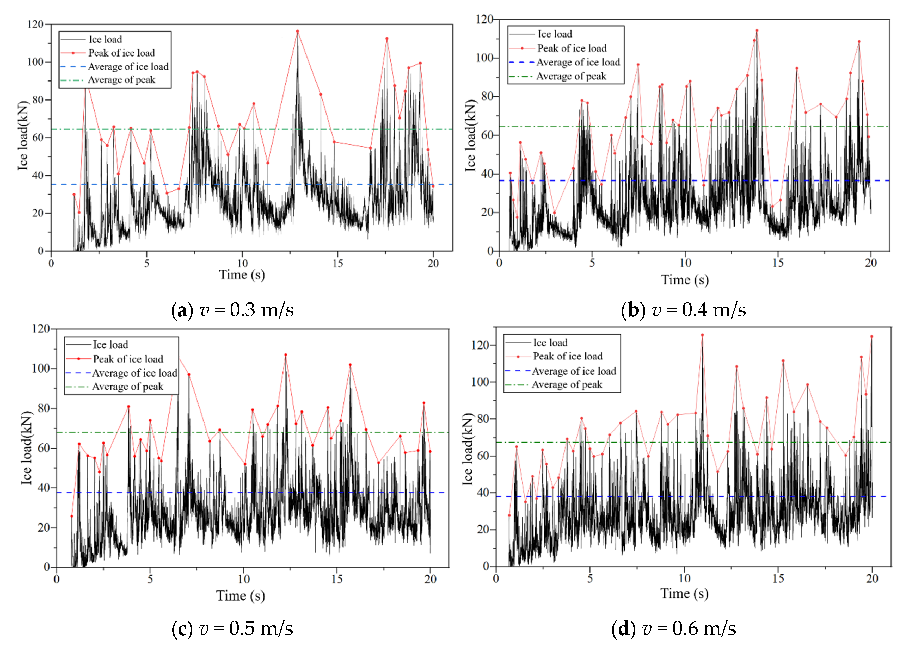
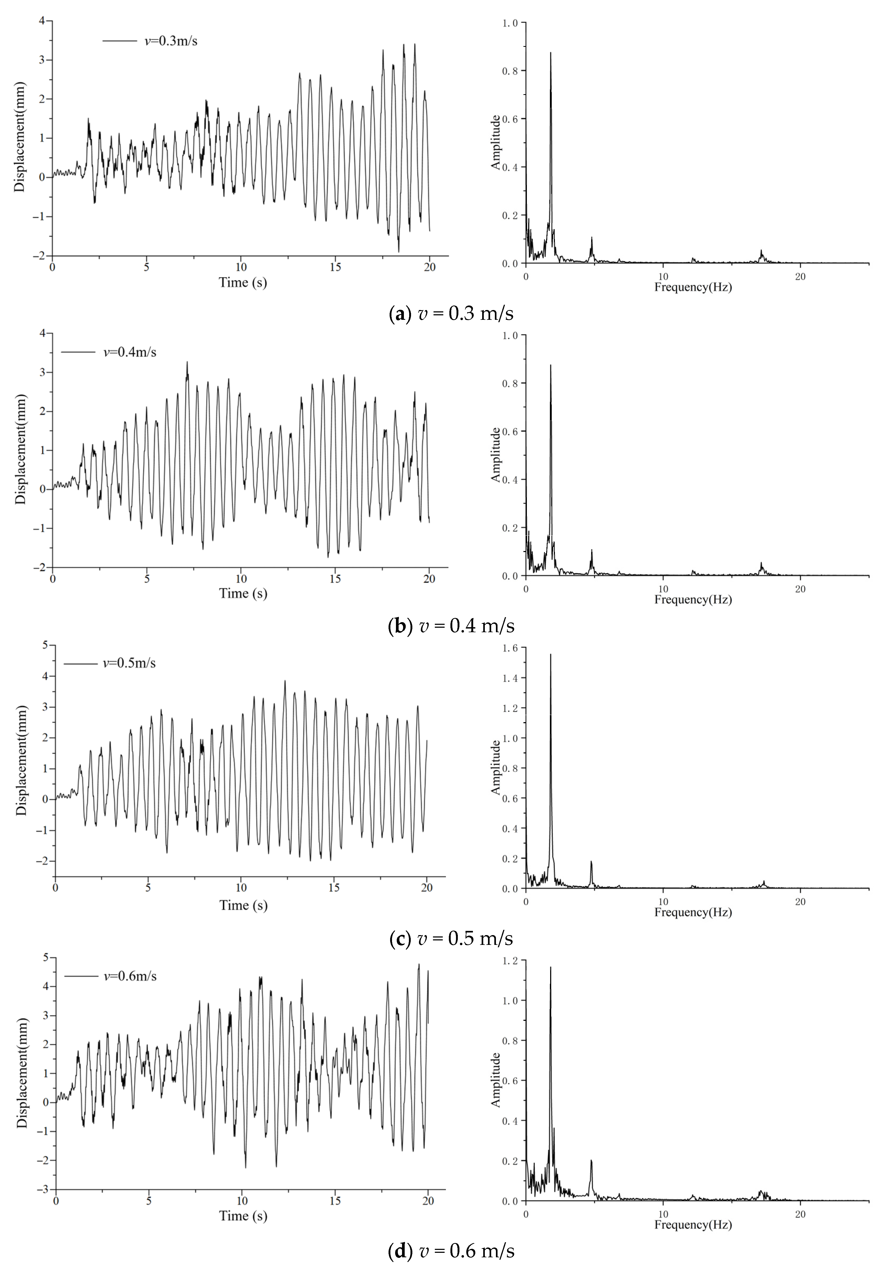
5.2. The Influence of Ice Velocity

In the modeling of sea ice dynamics, the effect of ice speed is significant and cannot be neglected. The ice load cycle is influenced by both the fracture length of the sea ice and the ice speed and, as previously discussed, the fracture length is directly proportional to the ice thickness. Our analysis of experimental data revealed that this ratio is not constant but is instead contingent upon the ice speed. The selected conditions for the ice are as follows: the compressive strength of the sea ice is 4.2 MPa, the flexural strength is 1.4 MPa, the ice thickness is 0.3 m, and the ice speeds are set at 0.3 m/s, 0.4 m/s, 0.5 m/s, and 0.6 m/s. The discrete element parameters associated with the sea ice speed can be found in

Table 2. Discrete element parameters of sea ice at different ice speeds.

Parameter	Value
Sea ice thickness h/m	0.3
Particle diameter D/mm	100
Cementation modulus PBN/MPa	759.1
Ratio of cemented tangential to normal stiffness PBS	0.574
Cementation normal bond strength PBN_S/MPa	0.519
Cementation tangential bond strength PBS_S/MPa	1.221
Friction coefficient of ice and structure ${\mu }_w$	0.15
Friction coefficient of particles ${\mu }_P$	0.1
Normal viscosity coefficient Cn	0.7
Tangential viscosity coefficient Cs	0.4

.

The ice load time-history curves at different ice speeds are shown in Figure 14. It can be observed that the peak ice load remains roughly around 120 kN across various ice speeds, with the average peak value and overall average value stabilizing at approximately 67 kN and 38 kN, respectively. This indicates that, compared to ice thickness, the effect of ice speed on the ice load is relatively minor. Moreover, this study primarily focuses on the brittle failure characteristics of sea ice, and the potential influence of the bonding strength between discrete element sea ice particles on loading rates was not considered in the simulation process. As a result, variations in speed did not significantly impact the final calculation results, a conclusion that aligns with related laboratory experiments and actual measurements [1,12,17,44,45].

The time-history curves and frequency spectrum of ice-induced vibration acceleration for the platform at different ice speeds are shown in Figure 15. The vibration acceleration exhibits a certain periodicity; however, the vibration period displays significant randomness. The ice-induced vibration acceleration of the platform increases with the rise in ice speed, but compared to ice thickness, the effect of ice speed on the ice-induced vibration acceleration is relatively minor.

The time-history curves of ice-induced vibration displacement for the platform at different ice speeds are shown in Figure 16. The ice-induced vibration displacement exhibits periodic changes that tend to increase with the rise in ice speed; however, it is important to note that these changes are not significant in magnitude. This behavior parallels that observed in the ice-induced vibration acceleration, suggesting a consistent relationship between speed and vibration characteristics. As the velocity of the ice increases, the system experiences variations in displacement that, while periodic, do not translate into drastic fluctuations, indicating a degree of stability in the platform’s response to ice movement. Specifically, the displacement natural frequencies corresponding to ice velocities of 0.3 m/s, 0.4 m/s, 0.5 m/s, and 0.6 m/s are measured at 0.55 mm, 1.16 mm, 1.55 mm, and 1.17 mm, respectively. These frequencies provide insight into the dynamic behavior of the platform as it interacts with moving ice, highlighting how varying speeds can influence the vibrational response. Moreover, the mean displacement values for these velocities are recorded as 0.008 mm, 0.008 mm, 0.010 mm, and 0.015 mm, respectively. These mean values, while also relatively small, reflect a gradual increase in displacement as ice speed rises, further supporting the observation of periodic changes in the system’s response to ice dynamics. Overall, the data underscore the complexity of the interaction between the platform and the ice, emphasizing the need for careful consideration in engineering and operational strategies.

Figure 17 shows the stress–time-history curve associated with the maximum stress cloud map on the surface of the conical shell plate. The stress generated in the conical shell plate shows minimal sensitivity to variations in ice speed. Because changes in ice speed have a negligible effect on the ice load borne by the shell plate’s surface, the resulting stress variations are also minimal. Furthermore, the maximum stress values remain well within the yield strength of the shell plate, indicating that it can adequately withstand impacts from sea ice at varying speeds. The investigation of ice-induced effects in the conical structure aligns with linear elastic analysis criteria across different ice conditions.

6. Conclusions

This work investigated the ice-induced vibration characteristics of a typical jacket platform in the Bohai Sea. The interactions between sea ice and the platform were simulated employing a new common-node DEM approach. Modal analysis was conducted on the jacket platform model, alongside measured inherent frequencies, to validate the dynamic characteristics of the simplified jacket model. Using a controlled variable method, the study examined the ice loads and ice-induced vibration characteristics of the JZ20-2NW platform’s conical structure under varying ice conditions, including ice thickness and ice speed. The following conclusions were drawn:

(1) The influence of ice thickness on the ice resistance mechanism of the conical structure is quite significant. The fracture length of sea ice increases with the thickness, and both the peak ice load and the peak ice-induced vibration acceleration are proportional to the square of the ice thickness, which is consistent with the experimental and field observation results.

(2) Ice thickness has a considerable impact on the displacement of ice-induced vibrations in the jacket platform. The positive displacement shows a clear upward trend with increasing ice thickness, while the negative displacement marginally changes, remaining around −1.5 mm.

(3) The ice-induced vibration acceleration and displacement of the conical structure and ice load both increase with increasing ice speed, although this effect is smaller compared to that of ice thickness.

(4) In the analysis of the strength of the conical shell plate, the ice load does not exceed the yield strength of the shell plate, and the yield strength of the shell plate is significantly greater than the peak stress, indicating that the traditional conical shell plate structure exhibits strength redundancy.

References

1. Brown, T.G.; Määttänen, M. Comparison of Kemi-I and Confederation Bridge cone ice load measurement results. Cold Reg. Sci. Technol. 2009, 55, 3–13. [Google Scholar] [CrossRef]
2. Wu, Q.-G.; Wang, Z.-C.; Ni, B.-Y.; Yuan, G.-Y.; Semenov, Y.A.; Li, Z.-Y.; Xue, Y.-Z. Ice-water-gas interaction during icebreaking by an airgun bubble. J. Mar. Sci. Eng. 2022, 10, 1302. [Google Scholar] [CrossRef]
3. Yuan, G.; Ni, B.; Wu, Q.; Lu, W.; Xue, Y. Experimental study on ice breaking by a cavitating water jet in a Venturi structure. Appl. Therm. Eng. 2024, 239, 122095. [Google Scholar] [CrossRef]
4. Yuan, G.-Y.; Ni, B.-Y.; Wu, Q.-G.; Xue, Y.-Z.; Han, D.-F. Ice breaking by a high-speed water jet impact. J. Fluid Mech. 2022, 934, A1. [Google Scholar] [CrossRef]
5. Ranta, J.; Polojärvi, A.; Tuhkuri, J. Ice loads on inclined marine structures—Virtual experiments on ice failure process evolution. Mar. Struct. 2018, 57, 72–86. [Google Scholar] [CrossRef]
6. Sinsabvarodom, C.; Leira, B.J.; Høyland, K.V.; Næss, A.; Samardžija, I.; Chai, W.; Komonjinda, S.; Chaichana, C.; Xu, S. On Statistical Features of Ice Loads on Fixed and Floating Offshore Structures. J. Mar. Sci. Eng. 2024, 12, 1458. [Google Scholar] [CrossRef]
7. Wang, B.; Yin, H.; Gao, S.; Qu, Y.; Chuang, Z. Ice-Induced Vibration Analysis of Fixed-Bottom Wind Turbine Towers. J. Mar. Sci. Eng. 2024, 12, 1159. [Google Scholar] [CrossRef]
8. Xu, Y.; Zhang, D.; Wu, K.; Peng, X.; Jia, X.; Wang, G. Study on the Factors Influencing the Amplitude of Local Ice Pressure on Vertical Structures Based on Model Tests. J. Mar. Sci. Eng. 2024, 12, 1634. [Google Scholar] [CrossRef]
9. Moslet, P.O. Field testing of uniaxial compression strength of columnar sea ice. Cold Reg. Sci. Technol. 2007, 48, 1–14. [Google Scholar] [CrossRef]
10. Timco, G.W.; Frederking, R. Probabilistic analysis of seasonal ice loads on the Molikpaq. In Proceedings of the 17th International Association of Hydraulic Engineering and Research (IAHR), Saint Petersburg, Russia, 21–25 June 2004; Volume 2, pp. 68–76. [Google Scholar]
11. Ji, S.; Di, S.; Liu, S. Analysis of ice load on conical structure with discrete element method. Eng. Comput. 2015, 32, 1121–1134. [Google Scholar] [CrossRef]
12. Yue, Q.; Bi, X. Ice-Induced Jacket Structure Vibrations in Bohai Sea. J. Cold Reg. Eng. 2000, 14, 81–92. [Google Scholar] [CrossRef]
13. Barker, A.; Timco, G. Beaufort sea rubble fields: Characteristics and implications for nearshore petroleum operations. Cold Reg. Sci. Technol. 2016, 121, 66–83. [Google Scholar] [CrossRef]
14. Barker, A.; Timco, G.; Gravesen, H.; Vølund, P. Ice loading on Danish wind turbines: Part 1: Dynamic model tests. Cold Reg. Sci. Technol. 2005, 41, 1–23. [Google Scholar] [CrossRef]
15. Hirayama, K.; Obara, I. Ice forces on inclined structure. In Proceedings of the 5th International Offshore Mechanics and Arctic Engineering, Tokyo, Japan, 13–18 April 1986; pp. 515–520. [Google Scholar]
16. Yue, Q.; Qu, Y.; Bi, X.; Tuomo, K. Ice force spectrum on narrow conical structures. Cold Reg. Sci. Technol. 2007, 49, 161–169. [Google Scholar] [CrossRef]
17. Yan, Q.; Yue, Q.; Bi, X.; Tuomo, K. A random ice force model for narrow conical structures. Cold Reg. Sci. Technol. 2006, 45, 148–157. [Google Scholar] [CrossRef]
18. Xu, N.; Yue, Q.; Bi, X.; Tuomo, K.; Zhang, D. Experimental study of dynamic conical ice force. Cold Reg. Sci. Technol. 2015, 120, 21–29. [Google Scholar] [CrossRef]
19. Tian, Y.; Huang, Y. The dynamic ice loads on conical structures. Ocean Eng. 2013, 59, 37–46. [Google Scholar] [CrossRef]
20. Xu, N.; Yue, Q.; Yuan, S.; Liu, X.; Shi, W. Classification criterion of narrow/wide ice-resistant conical structures based on direct measurements. J. Mar. Sci. Appl. 2016, 15, 376–381. [Google Scholar] [CrossRef]
21. Di, S.; Xue, Y.; Wang, Q.; Bai, X. Discrete element simulation of ice loads on narrow conical structures. Ocean Eng. 2017, 146, 282–297. [Google Scholar] [CrossRef]
22. Long, X.; Liu, S.; Ji, S. Discrete element modelling of relationship between ice breaking length and ice load on conical structure. Ocean Eng. 2020, 201, 107152. [Google Scholar] [CrossRef]
23. Ji, S.; Tian, Y. Numerical ice tank for ice loads based on multi-media and multi-scale discrete element method. Chin. J. Theor. Appl. Mech. 2021, 53, 2427–2453. [Google Scholar]
24. Lu, W.; Lubbad, R.; Løset, S.; Kashafutdinov, M. Fracture of an ice floe: Local out-of-plane flexural failures versus global in-plane splitting failure. Cold Reg. Sci. Technol. 2016, 123, 1–13. [Google Scholar] [CrossRef]
25. Su, B.; Riska, K.; Moan, T. A numerical method for the prediction of ship performance in level ice. Cold Reg. Sci. Technol. 2010, 60, 177–188. [Google Scholar] [CrossRef]
26. Hopkins, M.A. Onshore ice pile-up: A comparison between experiments and simulations. Cold Reg. Sci. Technol. 1997, 26, 205–214. [Google Scholar] [CrossRef]
27. Paavilainen, J.; Tuhkuri, J. Pressure distributions and force chains during simulated ice rubbling against sloped structures. Cold Reg. Sci. Technol. 2013, 85, 157–174. [Google Scholar] [CrossRef]
28. Jia, B.; Ju, L.; Wang, Q. Numerical Simulation of Dynamic Interaction Between Ice and Wide Vertical Structure Based on Peridynamics. Comput. Model. Eng. Sci. 2019, 121, 501–522. [Google Scholar] [CrossRef]
29. Liu, M.; Wang, Q.; Lu, W. Peridynamic simulation of brittle-ice crushed by a vertical structure. Int. J. Nav. Archit. Ocean Eng. 2017, 9, 209–218. [Google Scholar] [CrossRef]
30. Liu, R.; Xue, Y.; Han, D.; Ni, B. Studies on model-scale ice using micro-potential-based peridynamics. Ocean Eng. 2021, 221, 108504. [Google Scholar] [CrossRef]
31. Liu, R.; Xue, Y.; Lu, X. Coupling of Finite Element Method and Peridynamics to Simulate Ship-Ice Interaction. J. Mar. Sci. Eng. 2023, 11, 481. [Google Scholar] [CrossRef]
32. Liu, L.; Zhang, P.; Xie, P.; Ji, S. Coupling of dilated polyhedral DEM and SPH for the simulation of rock dumping process in waters. Powder Technol. 2020, 374, 139–151. [Google Scholar] [CrossRef]
33. Lu, W.; Lubbad, R.; Løset, S. Simulating Ice-Sloping Structure Interactions With the Cohesive Element Method. J. Offshore Mech. Arct. Eng. 2014, 136, 031501. [Google Scholar] [CrossRef]
34. Shen, H.H.; Hibler, W.D.; Leppäranta, M. On applying granular flow theory to a deforming broken ice field. Acta Mech. 1986, 63, 143–160. [Google Scholar] [CrossRef]
35. Tuhkuri, J.; Polojrvi, A. A review of discrete element simulation of ice-structure interaction. Philos. Trans. R. Soc. A Math. Phys. Eng. Sci. 2018, 376, 20170335. [Google Scholar] [CrossRef] [PubMed]
36. Xue, Y.; Liu, R.; Li, Z.; Han, D. A review for numerical simulation methods of ship–ice interaction. Ocean Eng. 2020, 215, 107853. [Google Scholar] [CrossRef]
37. Ji, S.; Di, S.; Long, X. DEM Simulation of Uniaxial Compressive and Flexural Strength of Sea Ice: Parametric Study. J. Eng. Mech. 2017, 143, C4016010. [Google Scholar] [CrossRef]
38. Huang, L.; Tuhkuri, J.; Igrec, B.; Li, M.; Stagonas, D.; Toffoli, A.; Cardiff, P.; Thomas, G. Ship resistance when operating in floating ice floes: A combined CFD&DEM approach. Mar. Struct. 2020, 74, 102817. [Google Scholar] [CrossRef]
39. Zhong-Xiang, S.; Wen-Qing, W.; Cheng-Yue, X.U.; Hong-Bin, L.I.; Yin, J.; Ren-Wei, L. Numerical Simulation of Sea Ice and Structure Interaction Using Common Node DEM-SPH Model. China Ocean Eng. 2023, 37, 897–911. [Google Scholar]
40. Wang, S.; Yue, Q.; Zhang, D. Ice-induced non-structure vibration reduction of jacket platforms with isolation cone system. Ocean Eng. 2013, 70, 118–123. [Google Scholar] [CrossRef]
41. Wu, W.H.; Yu, B.J.; Xu, N.; Yue, Q.J. Numerical simulation of dynamic ice action on conical structure. Eng. Mech. 2008, 25, 192–196. (In Chinese) [Google Scholar]
42. Ralston, T. Plastic limit analysis of sheet ice loads on conical structures. In Physics and Mechanics of Ice: Symposium Copenhagen, 6–10 August 1979, Copenhagen, Denmark; Technical University of Denmark: Lyngby, Denmark, 1979; pp. 289–308. [Google Scholar]
43. Kato, K.; Izumiyama, K. Simulation of ice loads on a conical shaped structure: Comparison with experimental results. In Proceedings of the ISOPE International Ocean and Polar Engineering Conference, Honolulu, HI, USA, 25–30 May 1997; p. ISOPE-I-97-207. [Google Scholar]
44. Frederking, R.; Schwarz, J. Model tests of ice forces on fixed and oscillating cones. Cold Reg. Sci. Technol. 1982, 6, 61–72. [Google Scholar] [CrossRef]
45. Wessels, E.; Kato, K. Ice forces on fixed and floating conical structures. In Proceedings of the 9th International IAHR Symposium on Ice, Sapporo, Japan, 23–27 August 1988; pp. 666–691. [Google Scholar]
Figure 1. Schematic diagram of common-node DEM-SPH particles.
Jmse 12 01999 g001
Figure 2. A schematic for model contact.
Jmse 12 01999 g002
Figure 3. The JZ20-2NW offshore platform.
Jmse 12 01999 g003
Figure 4. Illustration for sea ice and the JZ20-2NW platform interaction.
Jmse 12 01999 g004
Figure 5. Natural frequencies and modes of the first six modes of JZ20-2NW model.
Jmse 12 01999 g005
Figure 6. Interaction between sea ice and JZ20-2NW under different ice thicknesses.
Jmse 12 01999 g006
Figure 7. Ice load history of vertebral body structure under different ice thicknesses with 0.24, 0.30, 0.36 and 0.42 m.
Jmse 12 01999 g007aJmse 12 01999 g007b
Figure 8. Ice load versus ice thickness.
Jmse 12 01999 g008
Figure 9. Peak ice force obtained by simulation and formula under different ice thicknesses.
Jmse 12 01999 g009
Figure 10. Time-history curve of ice-induced vibration acceleration of deck platform under different ice thicknesses.
Jmse 12 01999 g010aJmse 12 01999 g010b
Figure 11. Relationship between peak acceleration of ice-induced vibration and ice thickness. (a) Ice-induced vibration versus ice thickness. (b) Ice induced vibration versus the square of ice thickness.
Jmse 12 01999 g011
Figure 12. Time-history curve of ice-induced vibration displacement for the JZ20-2NW platform at various ice thicknesses.
Jmse 12 01999 g012aJmse 12 01999 g012b
Figure 13. Time-history curve of surface stress of conical shell plate with different ice thicknesses.
Jmse 12 01999 g013
Figure 14. Ice load time-history curve at different ice speeds.
Jmse 12 01999 g014
Figure 15. Time-history curve of ice-induced vibration acceleration of deck platform at different ice speeds.
Jmse 12 01999 g015
Figure 16. Time-history curve of ice-induced vibration displacement of deck platform at different ice speeds.
Jmse 12 01999 g016
Figure 17. Time-history curve of surface stress of conical shell plate at different ice speeds with 0.3, 0.4, 0.5 and 0.6 m/s.
Jmse 12 01999 g017