CFD-DEM Simulation on the Main-Controlling Factors Affecting Proppant Transport in Three-Dimensional Rough Fractures of Offshore Unconventional Reservoirs

Abstract

Hydraulic fracturing is a pivotal technique in the development of offshore unconventional reservoirs. While current research has primarily focused on the longitudinal or transverse roughness of fractures, this study shifts the emphasis to their three-dimensional (3D) roughness characteristics. We present a quantitative analysis of proppant transport within 3D rough fractures of offshore unconventional reservoirs, utilizing computational fluid dynamics (CFD) and the discrete element method (DEM). Our results are validated against experimental data. This study focuses on the main-control factors on the transport of the proppant in rough fractures, including surface roughness, the ratio of lateral to longitudinal forces, the ratio of the proppant diameter to the fracture aperture, and the fracture inclination angle. The results indicate that the rough surface of the fracture has a significant impact on the transport of the proppant, reducing lateral transport distance while increasing the height of the sand dune. Notably, both the lateral transport distance and the height of the sand dune show a quadratic relationship with the fractal dimension of the fractures. In addition, when the ratio of lateral to longitudinal forces is less than one, an increase in fracture roughness significantly reduces the transport efficiency. Once the ratio exceeds one, the effect of fracture roughness on proppant transport becomes negligible. Furthermore, when the ratio of the proppant diameter to the fracture aperture is below 0.25, the roughness has a minimal effect on the lateral transport of the proppant. Our findings, especially the simulation of proppant behavior in realistic 3D fractures, offer a valuable reference point for predicting proppant distribution.

1. Introduction

Hydraulic fracturing plays a crucial role in the development of offshore unconventional reservoirs. It significantly enhances the complexity of the fracture network and expands stimulation reservoir volume, thereby substantially increasing oil and gas production [1,2]. Despite technological advancements, horizontal wells in offshore unconventional reservoirs continue to encounter the challenge of rapid production decline during the initial stages of production [3,4,5,6]. One of the reasons for this phenomenon is the nonuniform distribution of the proppant within the fracture network. The fracturing process in rock creates surfaces that are typically characterized by a rough texture [7,8,9]. Roughness characteristics of the fracture surface are an important cause of the nonuniform proppant distribution. Nonuniform placement of proppants can result in unfilled areas within the fractures. As production proceeds, these unfilled areas may gradually close, reducing the fracture conductivity.

Proppant transport into rough fractures is influenced by the flow characteristics and mechanical behavior of particles [10,11]. Raimbay et al. [12] demonstrated that surface roughness not only determines the flow path of the fluid but also affects the transport of the proppant. Huang et al. [13] further observed that in rough fractures, the interaction between the proppant and the fracture surface promotes an increase in flow turbulence, which helps to suspend more proppant in the fluid. The research by Gong et al. [14] found that in rough fractures, the transport and sedimentation characteristics of the proppant are significantly different from those in smooth fractures, with rough fractures increasing the collisions between particle and particle and between particle and wall. Under the condition of multiparticle sedimentation, particle–particle and particle–wall interactions further affect the hydrodynamic and mechanical behavior of the proppant [15]. This indicates that when the surface morphology of the fracture is complex, the flow of the fluid and the proppant within the fracture becomes more complex, potentially leading to the formation of local velocity gradients and vortices. In addition, when the proppant collides or rubs against the fracture surface, the roughness of the surface increases friction and leads to irregular collisions. These interactions significantly affect the deposition and suspension state of the proppant in the slurry, thereby affecting the uniform sedimentation of the proppant.

The smooth parallel-plate model represents the most fundamental model for the study of fluid flow within fractures. It is commonly utilized in the early stages of research to study the migration and distribution of the proppant within these fractures [16,17,18]. This model provides a basic model for fractures, but neglects the effects of surface roughness and contact area [19]. With the advent of more sophisticated characterization and measurement techniques, the quantification of fracture roughness has become more precise [20,21]. To analyze effect of fracture roughness on proppant transport, rough fracture models are often applied in the study of proppant transport [8,20,22,23]. Fracture surfaces in existing studies are obtained by scanning natural surfaces or generated by fractal theory [24,25]. Numerous studies have conducted in-depth analyses comparing the distribution and migration of the proppant in smooth parallel-plate models with those in rough fractures, revealing significant differences between planar and rough fractures. Suri et al. [26] used CFD-DEM to study the impact of fracture roughness on the transport and placement of a proppant. They observed that particle–particle and particle–wall interactions become dominant in rough fractures. Zhang et al. [27] studied the sedimentation pattern of a proppant in rough fractures with a two-dimensional fractal dimension. They found that more sand clusters can form in rough fractures, whereas such formations do not occur in the smooth parallel-plate model. Guo et al. [28] studied the transport and placement of a proppant in rough fractures with different three-dimensional fractal dimensions. They found that compared with smooth fractures, proppant migration ability and volume all enhance in rough fractures. However, their model mainly considered longitudinal roughness and failed to fully capture the three-dimensional characteristics of the fracture surface. In reality, fractures in rock masses are three-dimensional, and thus, two-dimensional parameters struggle to accurately represent their roughness. Additionally, for the transport and placement of the proppant in rough fractures, researchers have conducted extensive quantitative studies. Zhang et al. [29] studied how fracture roughness affects the transport and placement of the proppant in laboratory-scale rough fracture models. They found that proppant dunes are lower and longer in fractures with a greater fractal dimension. Gong et al. [30] identified that a critical ratio of approximately 1.9 between the fracture width and the mean particle diameter is essential for the occurrence of proppant bridging. Hu et al. [31] conducted a comprehensive study examining the impact of various factors such as the fracture surface’s fractal dimension, fracture width, proppant distribution, shear slip, and tortuous angle on the flow field dynamics. Zhou et al. [32] introduced a comparative model that distinguishes between planar and rough fractures. The model analyzes the properties of dunes under different velocities and fractal dimensions. From this, it can be seen that current quantitative studies primarily focus on the morphological analysis of proppant dunes in rough fractures. These studies have analyzed the deposition and transport processes for various combinations of proppant sizes and injection parameters within rough fractures. However, the quantitative study of fracture roughness remains incomplete, and existing methods still exhibit limitations in their ability to quantitatively generate fractures with specific roughness characteristics.

In summary, existing studies have primarily focused on the longitudinal or transverse roughness of fractures, failing to capture the three-dimensional characteristics and not fully simulating the complex morphology of the fracture surface. Additionally, the effects of roughness on proppant transport and placement, as well as the role of the main-control factors, have not been fully explored and require further investigation. In this work, we employ the coupled CFD-DEM method to analyze the transport of a proppant in rough fractures. We generated 3D rough fracture models using a numerical synthesis method, based on parameters from real rough fractures. The focus is to explore the influence of the main-control factors on proppant transport in rough fractures. The rest of the paper is organized as follows. First, we construct the three-dimensional fracture model using the numerical synthesis method, which allows adjusting roughness through fractal dimension to accurately characterize real fracture roughness. Then, we use CFD-DEM to simulate proppant transport and distribution in rough fractures. Specifically, we quantitatively analyze the transport and distribution mechanisms of proppants in rough fractures, discussing main-control factors including the ratio of lateral to longitudinal forces, the ratio of particle diameter to fracture aperture, and the fracture inclination angle. The results of our research provide a reference point for estimating the distribution of proppants during hydraulic fracturing. This development enables a more precise prediction of proppant placement, which is essential for optimizing the efficacy of hydraulic fracturing in offshore unconventional reservoirs.

2. Methodology

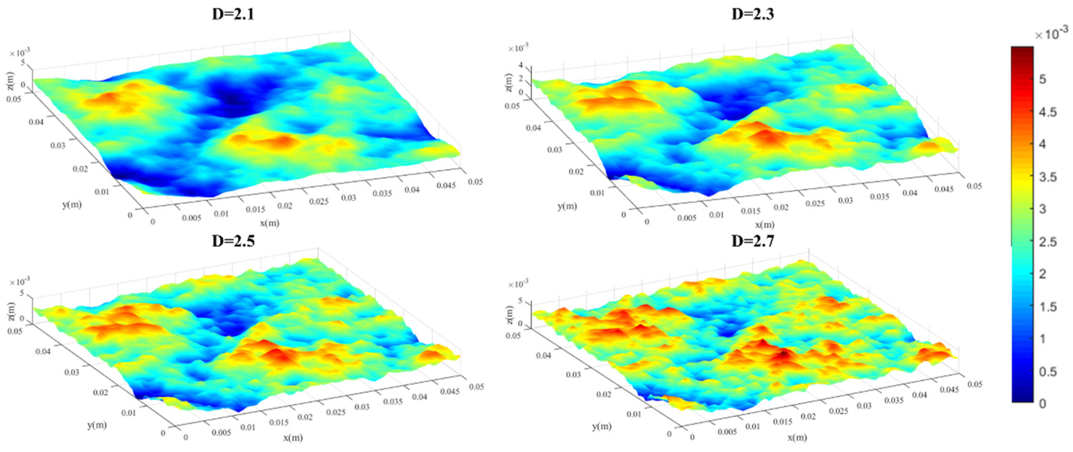
2.1. Construction of Rough Fractures Using Numerical Synthesis Method

The distinctive feature of fracture surfaces is their intricate and nonuniform topography. At the laboratory scale, hydraulic fracture surfaces have been observed to have fractal properties [33]. Fractal dimension, as a mathematical tool, is used to describe complex geometric shapes with irregular and self-similar characteristics. The fractal dimension transcends the traditional Euclidean dimensions, encapsulating the nuanced texture and multiscale complexity of the fractures [34,35]. Fractal dimensions between 2 and 3 are typical for naturally occurring rough surfaces, while smoother surfaces have dimensions close to 2 [36,37]. Fractal dimension captures not only the macroscopic two-dimensional properties of fractures, but also the more complex three-dimensional structure. As illustrated in Figure 1, the increase in fractal dimension is directly correlated with the enhanced roughness of the fracture surface. In this work, we use a numerical synthesis approach to generate rough fractures quantitatively. The method allows for the adjustment of the fractal dimension through parametric modeling, and accurately simulates the irregularities and roughness of fractures. By generating fractures with similar shapes, we can exclude the influence of the fracture shape on the results.

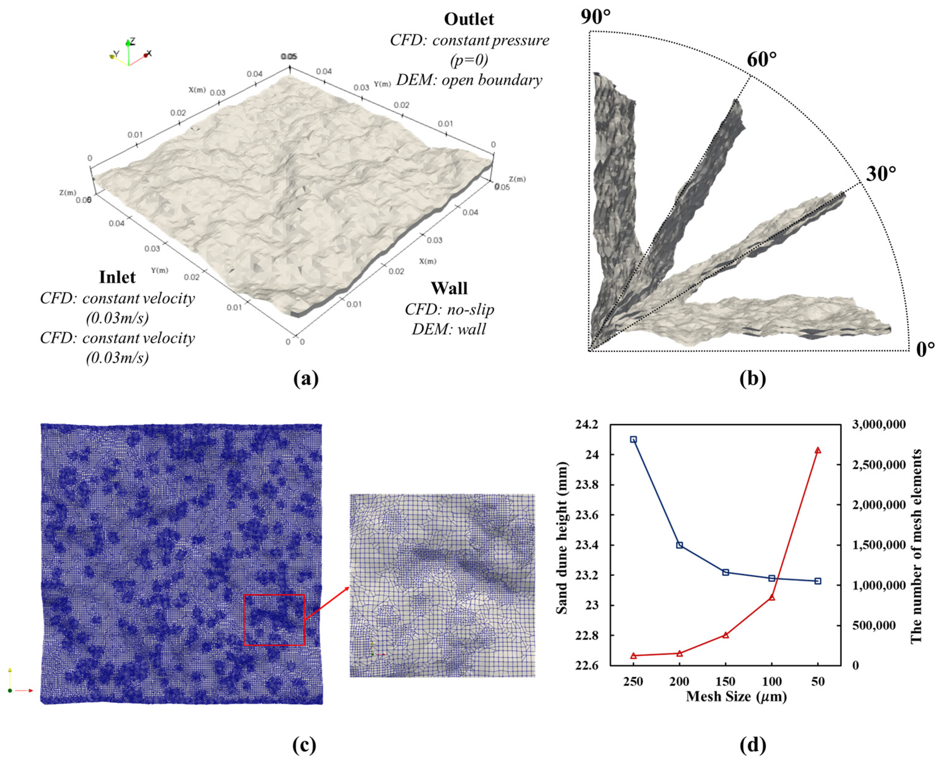
2.2. CFD-DEM Coupling Approach

The resolved CFD-DEM approach is applied to simulate proppant transport within rough fractures. In the resolved CFD-DEM method, a two-way coupling approach is adopted to encompass the dynamics of fluid–particle, particle–fluid, particle–particle, and particle–wall interactions. The motion of particles and the flow of fluid are coupled by treating each particle as a boundary condition. Two open-source solvers, OpenFOAM and LIGGGHTS, are used to numerically simulate fluid flow and particulate transport [38,39]. OpenFOAM, using the finite volume method (FVM), tackles the solution of the Navier–Stokes equations and the spatiotemporal discretization within the framework of computational fluid dynamics (CFD). The continuity equation is

$${\displaystyle \frac{\partial {\alpha }_f}{\partial t}}+\mathsf{\nabla }\cdot \left({\alpha }_f{u}_f\right)=0$$

(1)

where ${\alpha }_f$ is the volume fraction of the fluid phase; ${\displaystyle \frac{\partial {\alpha }_f}{\partial t}}$ is the partial derivative of the fluid volume fraction with respect to time; and $\mathsf{\nabla }\cdot \left({\alpha }_f{u}_f\right)$ is the divergence of the product of fluid volume fraction and fluid velocity vector. The momentum conservation equation (N-S equation) for the fluid phase is

$${\displaystyle \frac{\partial \left({\alpha }_f{u}_f\right)}{\partial t}}+\mathsf{\nabla }\cdot \left({\alpha }_f{u}_f\otimes u_f\right)=-{\alpha }_f\mathsf{\nabla }{\displaystyle \frac{P}{{\rho }_f}}+\mathsf{\nabla }\cdot \left({\alpha }_f\tau \right)+{\alpha }_{f}g-F_P$$

(2)

where ${\displaystyle \frac{\partial \left({\alpha }_f{u}_f\right)}{\partial t}}$ is the partial derivative of the product of the fluid volume fraction and fluid velocity vector with respect to time; $\mathsf{\nabla }\cdot \left({\alpha }_f{u}_f\otimes u_f\right)$ is the divergence of the outer product of the fluid velocity vector with itself, multiplied by the fluid volume fraction; $-{\alpha }_f\mathsf{\nabla }{\displaystyle \frac{P}{{\rho }_f}}$ is the negative product of the fluid volume fraction, gradient of pressure, and inverse of fluid density; $\mathsf{\nabla }\cdot \left({\alpha }_f\tau \right)$ is the divergence of the product of the fluid volume fraction and stress tensor; ${\alpha }_{f}g$ is the product of the fluid volume fraction and gravitational acceleration vector; and $F_P$ is the particle-phase force per unit volume.

The LIGGGHTS solver uses the DEM method to calculate particle location and velocity. For the coupling between fluid flow and particle motion, the resolved CFD-DEM method is used in this model to calculate the momentum exchange between fluid and particles. In the DEM approach, based on Newton’s second law, the governing equation for the motion of particle with mass $m_{p,i}$ can be presented as

$$m_{p,i}{\displaystyle \frac{d{u}_{p,i}}{dt}}=m_{p,i}{\ddot{X}}_{p,i}=F_{c,i}+F_{f,i}+F_{p,i}+F_{v,i}+F_{b,i}$$

(3)

where $u_{p,i}$ is the mass of the particle; $X_{p,i}$ is the time derivative of the velocity of particle; ${\displaystyle \frac{d{u}_{p,i}}{dt}}$ is acceleration of the particle; $F_{c,i}$ is the contact force on the particle, which includes normal and tangential components; $F_{f,i}$ is the drag force on the particle; $F_{p,i}$ is the pressure gradient force on the particle; $F_{v,i}$ is the viscous force on the particle; and $F_{b,i}$ is the buoyancy force on the particle. The Hertz model is used to calculate the particle–particle and particle–wall contact force [40,41]

$$F_{c,i}=F_{n,i}+F_{t,i}=\left(k_n\delta n_{ij}-{\gamma }_n\Delta u_{p,i}{n}_{ij}\right)+\left(k_t\delta t_{ij}-{\gamma }_t\Delta u_{p,i} t_{ij}\right)$$

(4)

where $F_{n,i}$ is the normal contact force component on the particle; $F_{t,i}$ is the tangential contact force component on the particle; $k$ and $\gamma$ are the elastic and viscoelastic constants; respectively; $n$ and $t$ are the unit vectors in the normal and tangential direction; respectively; $\Delta u_{p,i}$ is the relative velocity with respect to particle i; and $\delta$ is the overlap distance between two particles that are under contact. The Di Felice model [42] is adopted to calculate the fluid drag force

$$F_{f,i}={\displaystyle \frac{1}{2}}{\rho }_f\left(\left|u_{f,p}-u_{p,i}\right|\left(u_{f,p}-u_{p,i}\right)\right)C_{d,i}{\displaystyle \frac{\pi d_{p,i}^2}{4}}{\alpha }_f^{2-\mathsf{\chi }}$$

(5)

$$C_{d,i}=\left(0.63+{\displaystyle \frac{4.8}{R{e}_i^{0.5}}} \right)$$

(6)

$$R{e}_i={\displaystyle \frac{{\rho }_f{d}_{p,i}{\alpha }_f\left|u_{f,p}-u_{p,i}\right|}{{\mu }_f}}$$

(7)

$$\mathsf{\chi }=3.7-0.65\exp \left[-{\displaystyle \frac{{\left(1.5-lgR{e}_i\right)}^2}{2}}\right]$$

(8)

where $C_{d,i}$ is the drag coefficient; $R{e}_i$ is the Reynolds number for particle fluid density; $\left|u_{f,p}-u_{p,i}\right|$ is the absolute value of the difference between the fluid velocity and particle velocity; $d_{p,i}$ is the diameter of the particle; ${\mu }_f$ is the dynamic viscosity of the fluid; and $\mathsf{\chi }$ is a correction factor for the drag coefficient. The viscous force and pressure gradient force acting on particle i are calculated by

$$F_{v,i}=-\left(\mathsf{\nabla }·{\tau }_f\right)V_{p,i}$$

(9)

$$F_{p,i}=-\left(\mathsf{\nabla }p\right)V_{p,i}$$

(10)

where $\left(\mathsf{\nabla }·{\tau }_f\right)$ is the divergence of the fluid stress tensor; $V_{p,i}$ is the volume of the particle; and $\mathsf{\nabla }p$ is the gradient of pressure.

3. Numerical Model Verification and Simulation Setup

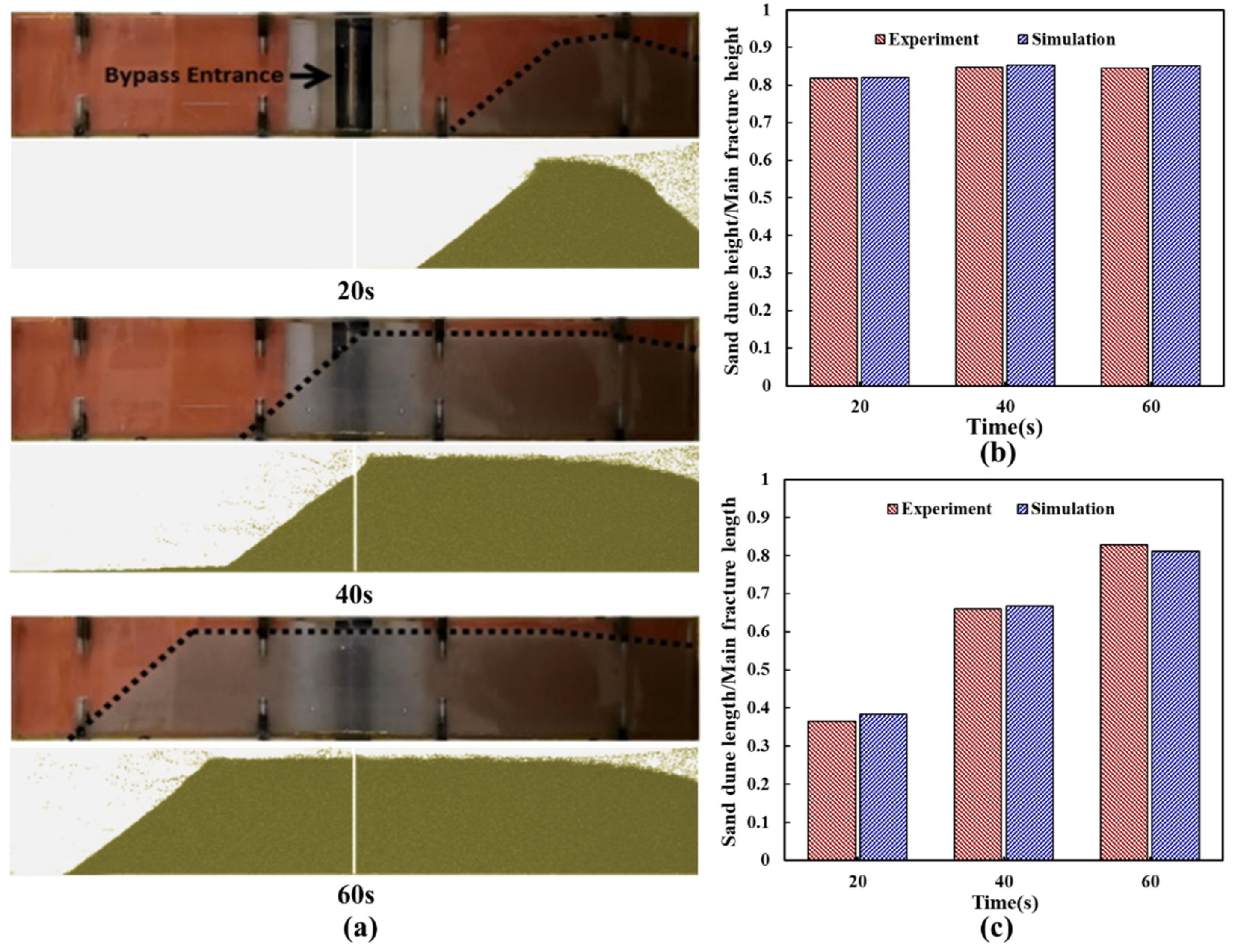
3.1. Numerical Model Verification

To ensure the accuracy of the model, we compared it with experimental data [43]. All conditions were the same as in the laboratory experiments except for the particle size of the proppant. The particle size distribution of the 20/40 mesh sand used in the experiments ranged from 0.4 to 0.8 mm. In the simulation, the midpoint of this range (0.6 mm) was chosen as the representative diameter of the proppant, and the other parameters are detailed in

Table 1. List of parameters used for model validation.

Parameter	Range
Main Fracture Length (mm)	381
Fracture Height (mm)	190.5
Fracture Width (mm)	2
Cross Corner Angle (°)	90
Proppant Diameter (mm)	0.6
Proppant Density (kg/m3)	2650
Proppant Concentration (vol. fraction)	0.038
Injection Velocity (m/s)	0.1
Fluid Viscosity (mPa·s)	1

.

Figure 2a shows the comparison between the experimental and simulation results for proppant distribution. The simulation results are very close to the experimental results, especially in the proppant transport process and dune shape changes. Figure 2b,c compare the height and length of proppant dunes between the experimental results and simulation data. The differences between the simulated and experimental results at various times are less than 2%. The minor discrepancies between the simulation results and the experimental data are attributed to the simplifications made in our model, specifically regarding the injection inlet and the bypass inlet. Therefore, our model can be used to accurately predict the transport and placement of proppants in fractures.

3.2. Simulation Setup

In this work, the open-source software SynFrac v1.0 is used to generate hydraulic fracture models with different fractal dimensions [44,45]. Fractal dimensions for the rough fractures are set at 2.1, 2.3, 2.5, and 2.7. Additionally, to provide a comparative baseline, a smooth fracture model is generated with a fractal dimension of 2.0. A representative size of fractures is chosen based on the actual dimensions of the fractures and the proppant, as well as the results of previous studies [13,14,46]. The average aperture of these fractures is established at 1 mm, with the fracture dimensions standardized to 50 mm by 50 mm. Figure 3 presents the rough fractures used in this study. It can be seen that that as the fractal dimension increases, the roughness of the fracture surface becomes more pronounced.

The boundary conditions for the CFD and DEM domains are shown in Figure 4a. The CFD domain is designed to maintain a uniform inlet fluid velocity, and to use a zero-pressure boundary condition for the outlet. The fracture walls and their adjacent sides are subjected to no-slip boundary conditions. For the DEM domain, the inlet particle velocity maintains at a constant and the outlet configures as an open boundary condition, allowing particles to exit the domain freely. The fracture walls and their adjacent sides are treated as wall boundaries, in accordance with the physical constraints on particle movement. Moreover, each fracture model is designed with different inclination angles as illustrated in Figure 4b. To enhance computational efficiency, localized mesh refinement has been implemented in areas where roughness changes significantly (Figure 4c). The mesh size was selected to be 125 μm, based on sensitivity analysis of the mesh (Figure 4d). To ensure the accuracy of the calculation results, the mesh has been rigorously checked and optimized. The quality of the optimized mesh has been significantly improved. We have ensured that the minimum orthogonal quality of the mesh is greater than 0.2, the skewness values are all controlled within the range of 0 to 0.25, and the aspect ratios are all close to 1. Additionally, to better capture the flow characteristics of the boundary layer, we encrypted the boundary layer mesh. Specifically, we adjusted the height of the first cell near the wall to 5 × 10⁻⁴ m. This measure helps to maintain the YPLUS value near the wall at approximately 1, thus ensuring the simulation accuracy of the near-wall flow. The CFD time step is set at 10⁻⁴ s, while the DEM time step is set to 10⁻⁶ s. The number of coupling iterations between the CFD and DEM solvers is 100. The overall duration of the simulation is 10 s. The computational expense for each model is approximately 20 h.

The fluid injection velocity and the particle velocity are both set at a uniform value of 0.03 m/s, with the particle density defined as 2650 kg/m³. This study specifies a variety of particle diameters: 250 μm, 500 μm, and 750 μm. These parameter settings are designed to simulate the dynamic behavior of the fluids and the proppant during the actual hydraulic fracturing. The Reynolds number of the fluid during the proppant injection process is approximately 580. This value indicates that the flow within the fracture is mainly in a laminar state. Under laminar flow conditions, the fluid flow is relatively stable, with no significant turbulence.

Table 2. Physical and numerical parameter settings in the simulation.

Parameter	Range
Fracture Length (mm)	50
Fracture Width/Height (mm)	50
Equivalent Hydraulic Aperture (mm)	1
Fracture Fractal Dimension	2.1, 2.3, 2.5, 2.7
Proppant Size (mm)	0.25, 0.5, 0.75
Proppant Density (kg/m3)	2650
Proppant Concentration (vol. fraction)	0.05
Injection Velocity (m/s)	0.03
Fluid Viscosity (mPa·s)	1, 2, 3, 4, 5
Inclination Angle (°)	0, 30, 60, 90

presents the simulation parameters used in this work.

4. Results and Discussion

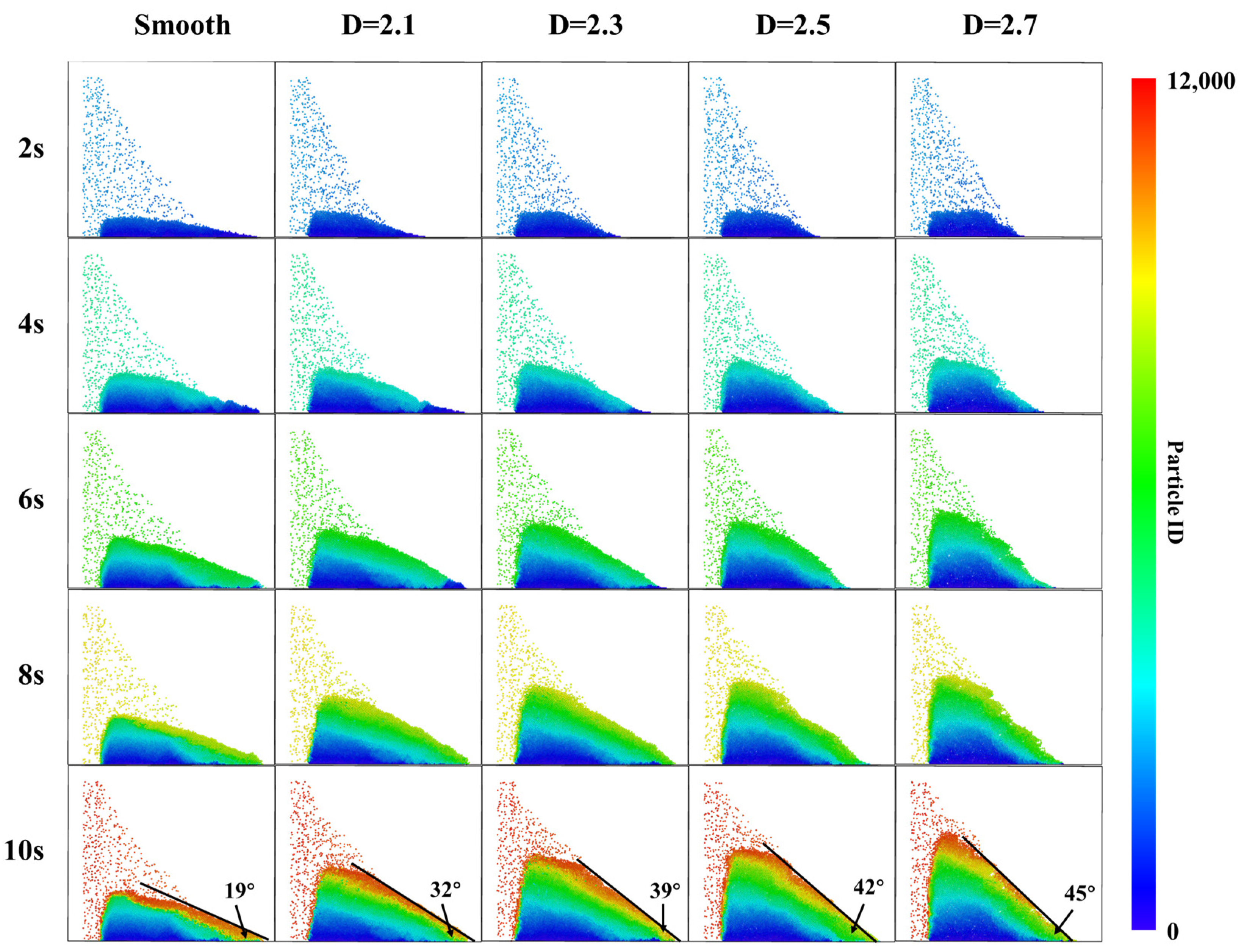
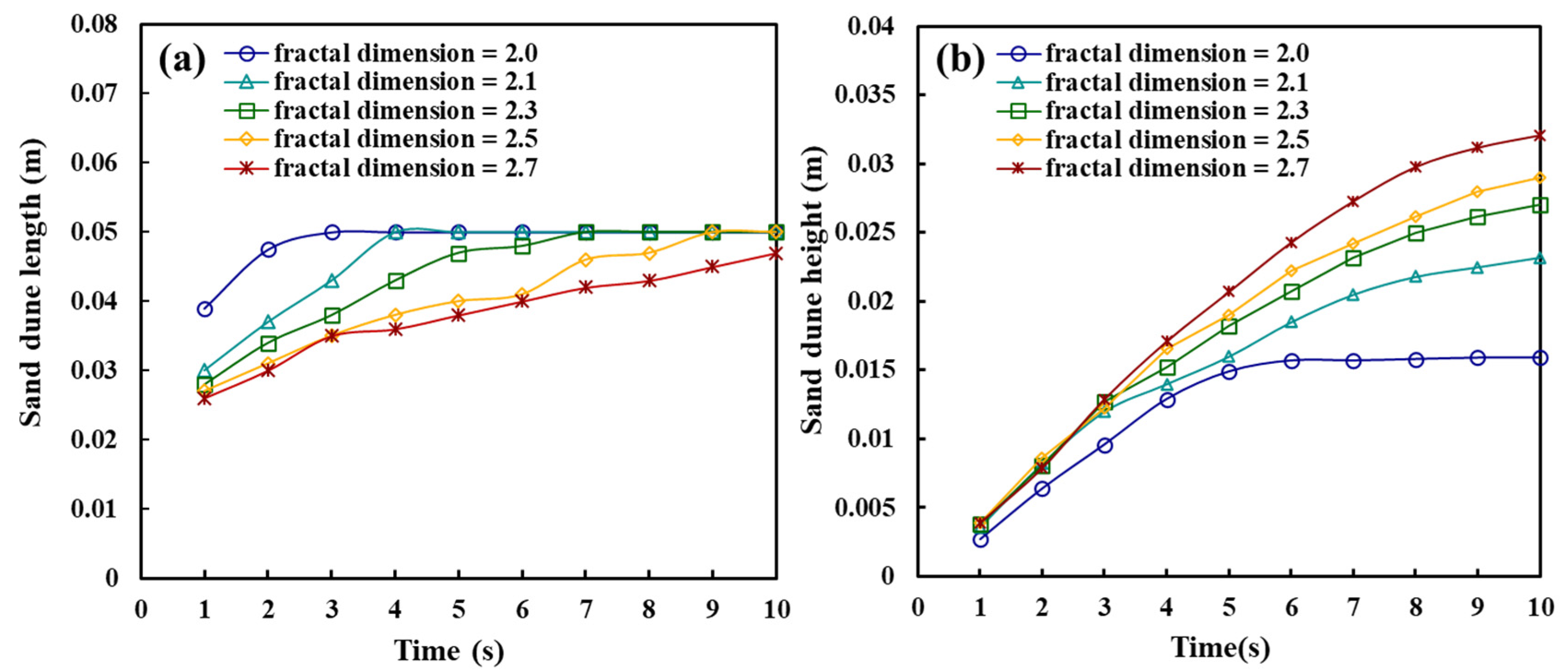
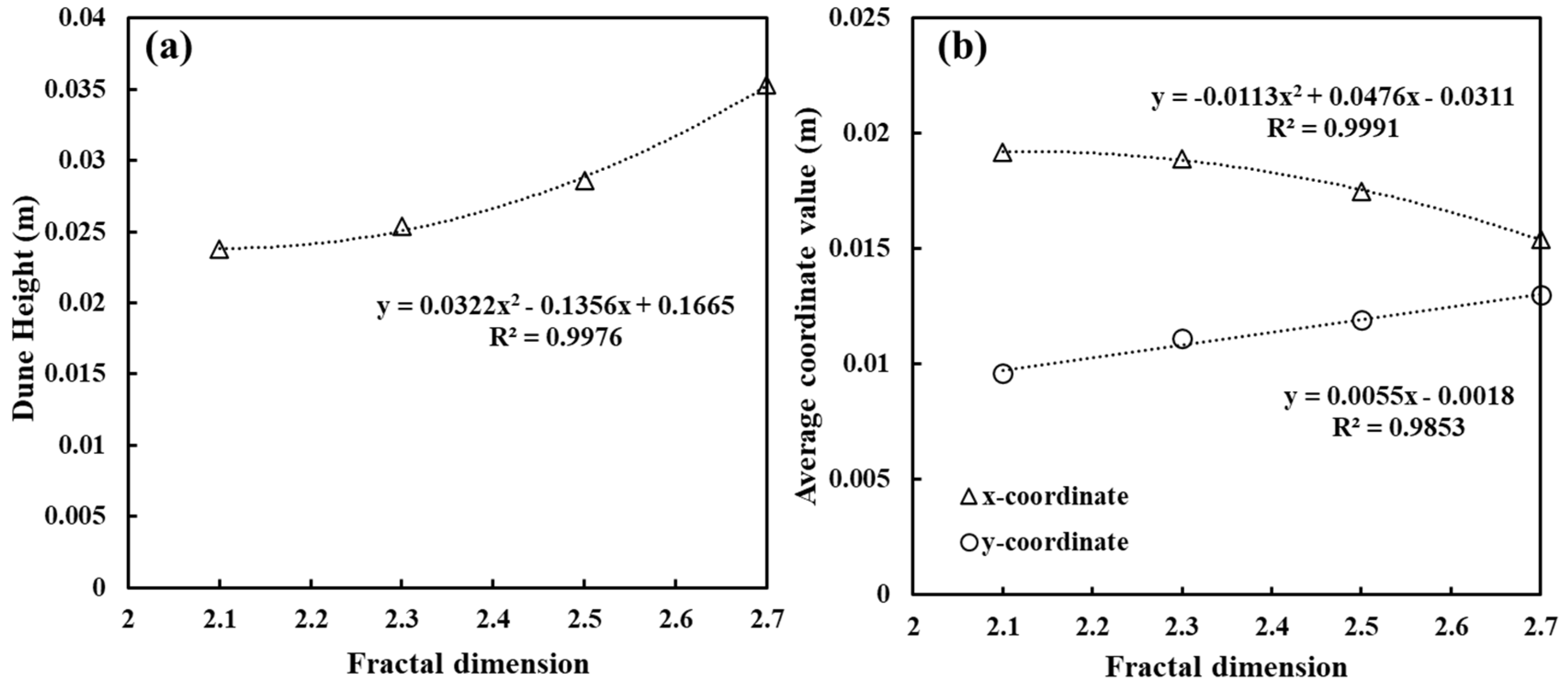
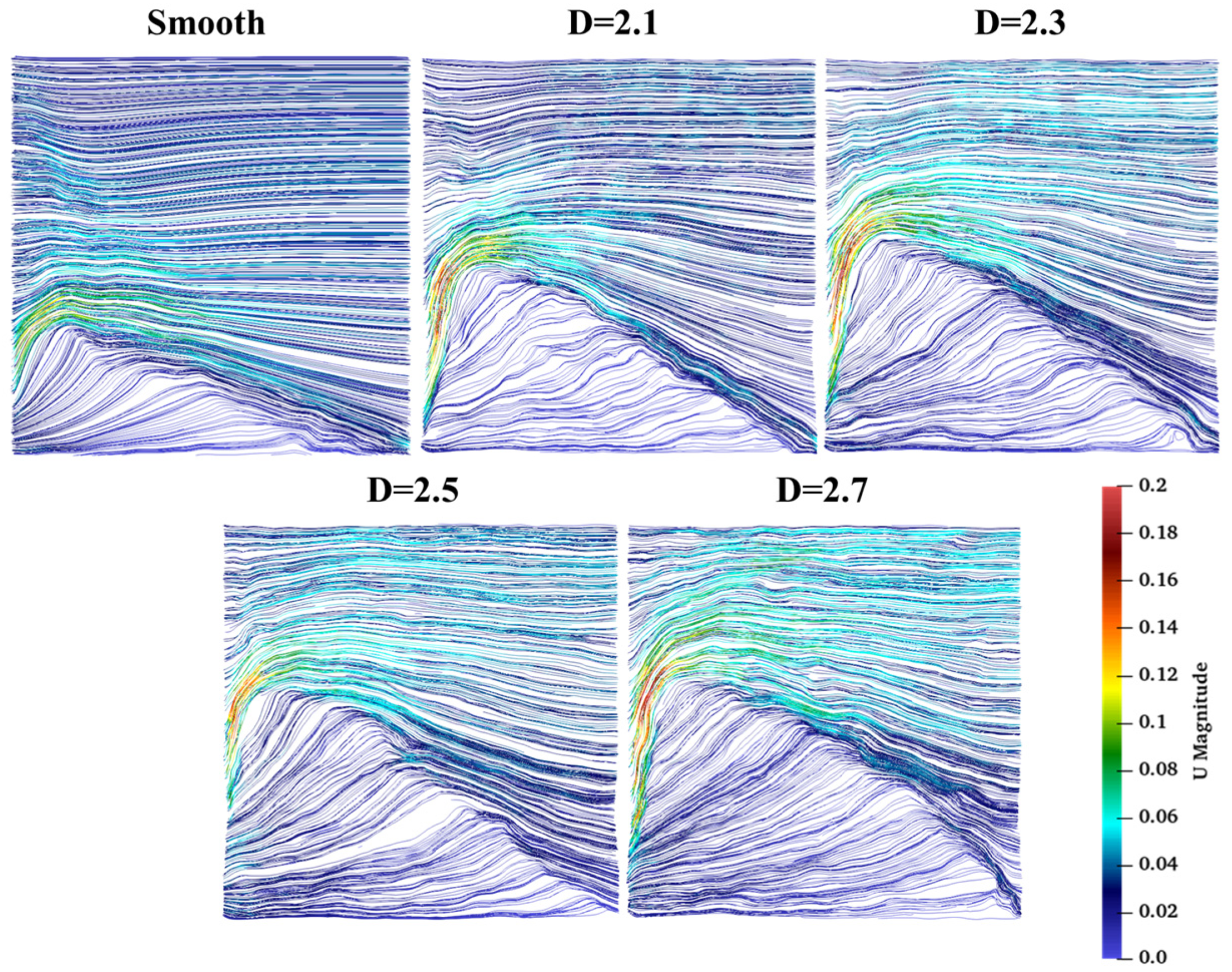
4.1. Proppant Transport in Vertical Fractures with Varying Roughness

In this section, we analyze proppant transport in vertical fractures with varying roughness, focusing on the generation processes of the proppant dune, the proppant transport distance, and the average velocity. The flow of slurry in vertical fractures can be disturbed by rough surfaces, which affect the transport and placement of the proppant, leading to the formation of sand dunes. Sand dunes, in turn, affect the flow characteristics of the slurry, resulting in a complex interaction between the slurry and the fracture.

Figure 5 illustrates that in a smooth fracture, proppant dunes tend to be shorter in height but longer in length than those in rough fractures. As the fractal dimension of rough fractures increases, the resulting proppant dunes become taller and shorter. Additionally, it is evident that the proppant tends to accumulate near the injection surface in rough fractures, rather than being uniformly distributed along the fracture length. The phenomenon can be attributed to the heightened frequency of particle–particle and particle–wall collisions in the rough fractures. Thus, in fractures with higher fractal dimensions, the back angle of sand dunes is steeper. This makes the proppant more susceptible to gravitational forces, leading to a more pronounced rolling.

We further analyze the change of the dune height with the injection time. In Figure 6a, it is observed that the time for the dunes to reach the outlet of the fracture increases with an increasing fractal dimension, indicating that the fracture roughness hinders the lateral transport of the proppant. As shown in Figure 6b, the dune height increases with the injection time, gradually reaching an equilibrium value. The time to reach the equilibrium dune height increases with the fractal dimension. An integrated analysis of Figure 5 and Figure 6 reveals that the sedimentation process of the proppant can be divided into two stages. In stage one, particle sedimentation is mainly governed by gravity, leading to a rapid increase in the dune height. Upon entering stage two, as the dune height increases, the slurry flow channel narrows and the flow rate accelerates. The rate of proppant sedimentation decreases and dune growth slows down until the dune height reaches its equilibrium value.

To explore the relationship between the fractal dimension of fractures and proppant transport efficiency, we analyze correlations between the fractal dimension, dune height, and the position of the proppants. Figure 7a shows that the dune height increases, and a quadratic relationship between the fractal dimension and the dune height occurs. In Figure 7b, there is a quadratic relationship between the fractal dimension and the average x-coordinate. A linear relationship exists between the fractal dimension and the average y-coordinate. As the fractal dimension increases, the average y-coordinate rises, while the average x-coordinate decreases.

To understand the effect of fractal dimension on the transport of the proppant at different stages, Figure 8 plots the changes in the average velocity of proppants in fractures with varying fractal dimensions. We define the average x-velocity of all proppants in the fluid domain as the lateral transport velocity and the average y-velocity is taken as the settling velocity. During stage one, the average x- and y-velocities of the proppant decrease until they reach equilibrium values in each fracture. Fractures with a higher fractal dimension tend to have a lower average x-velocity. While the average y-velocity remains the same with different fractal dimensions. In stage two, the average x- and y-velocities of the proppant are equilibrium, with fractures having a higher fractal dimension exhibiting a lower average velocity.

In order to clarify the transport mechanisms of the proppant, we conducted a detailed analysis on the streamlines and the dynamics of proppant movement. Figure 9 compares the streamlines in fractures with different fractal dimensions. The accumulation of proppant narrows the injection channel and causes significant fluctuations of fluid. The frequency of particle–particle and particle–wall collisions increase as the complexity of the fluid increases.

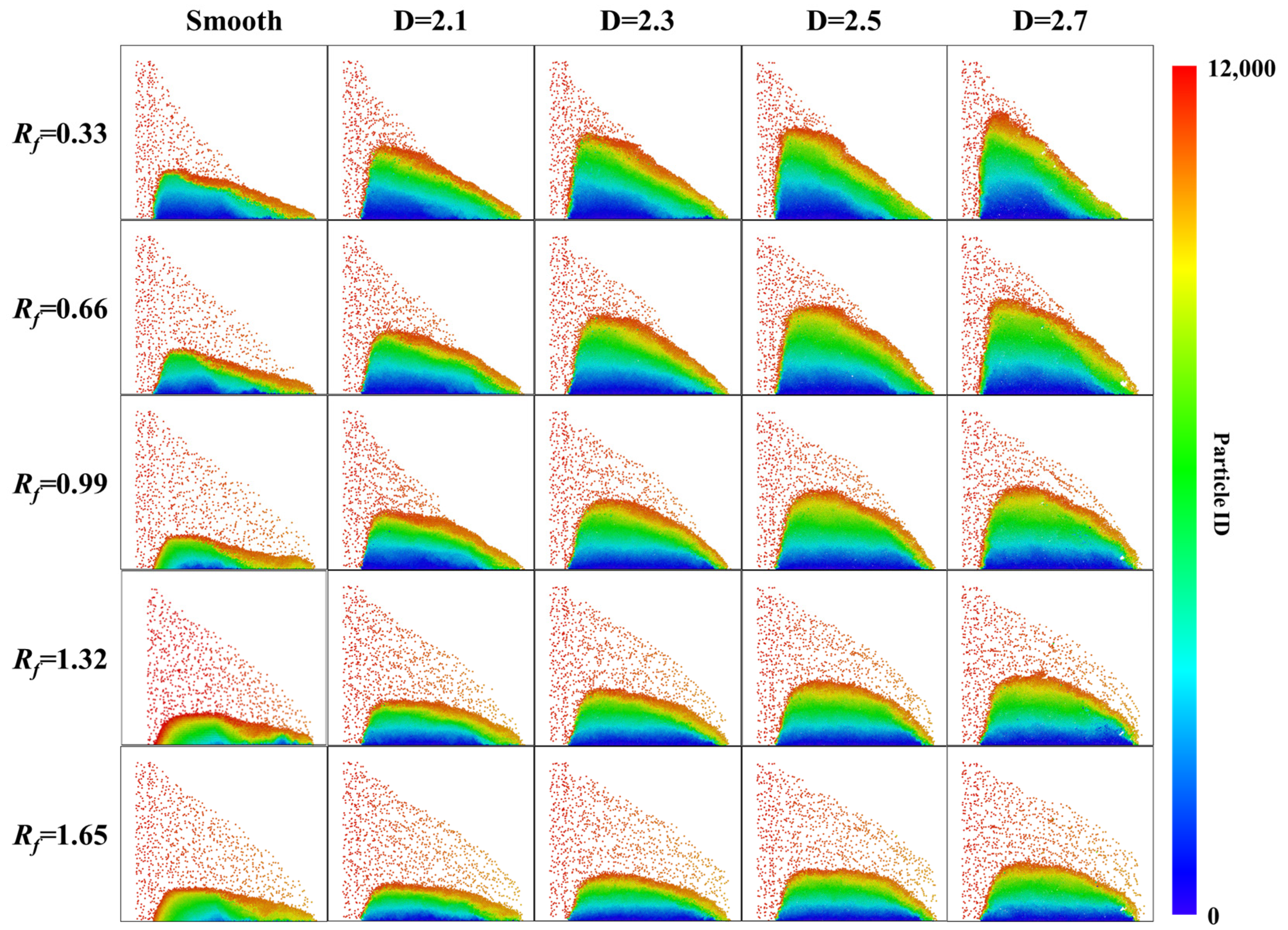
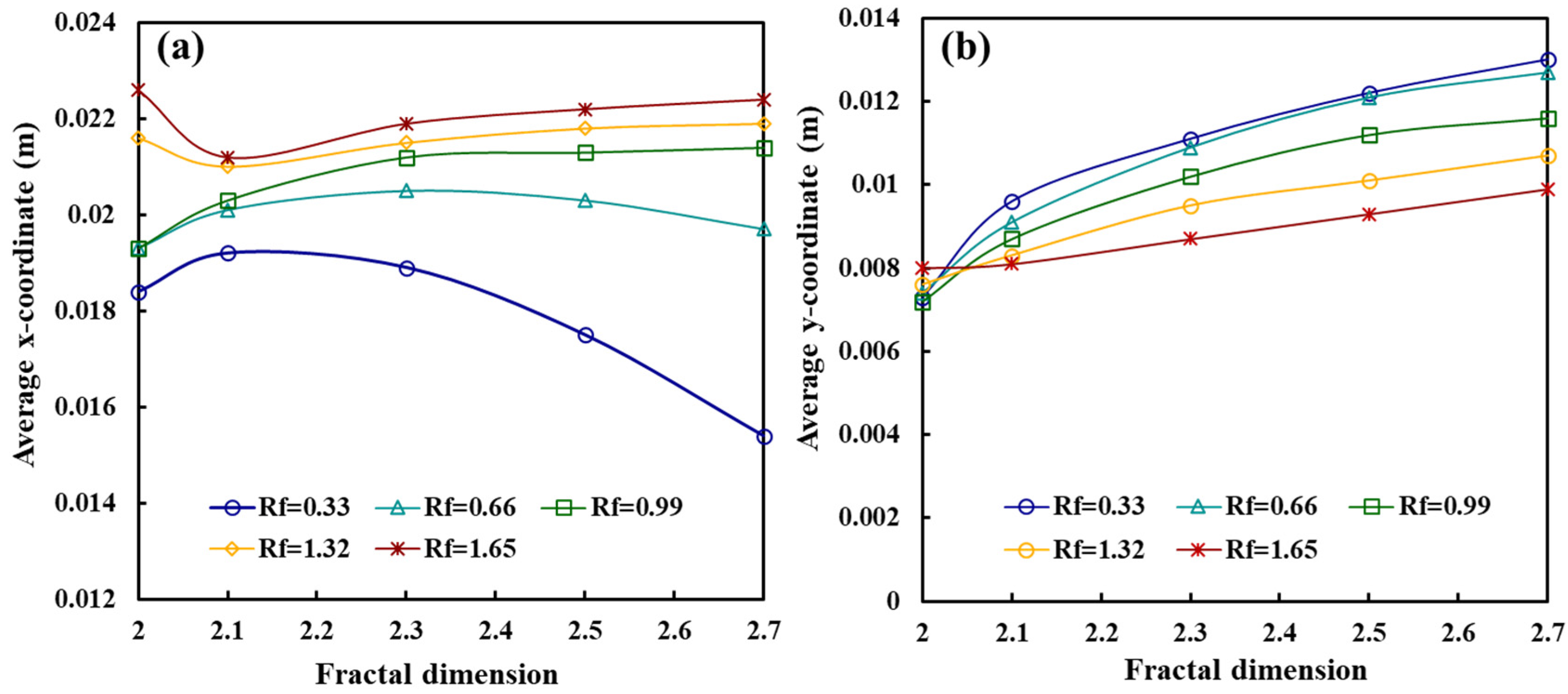
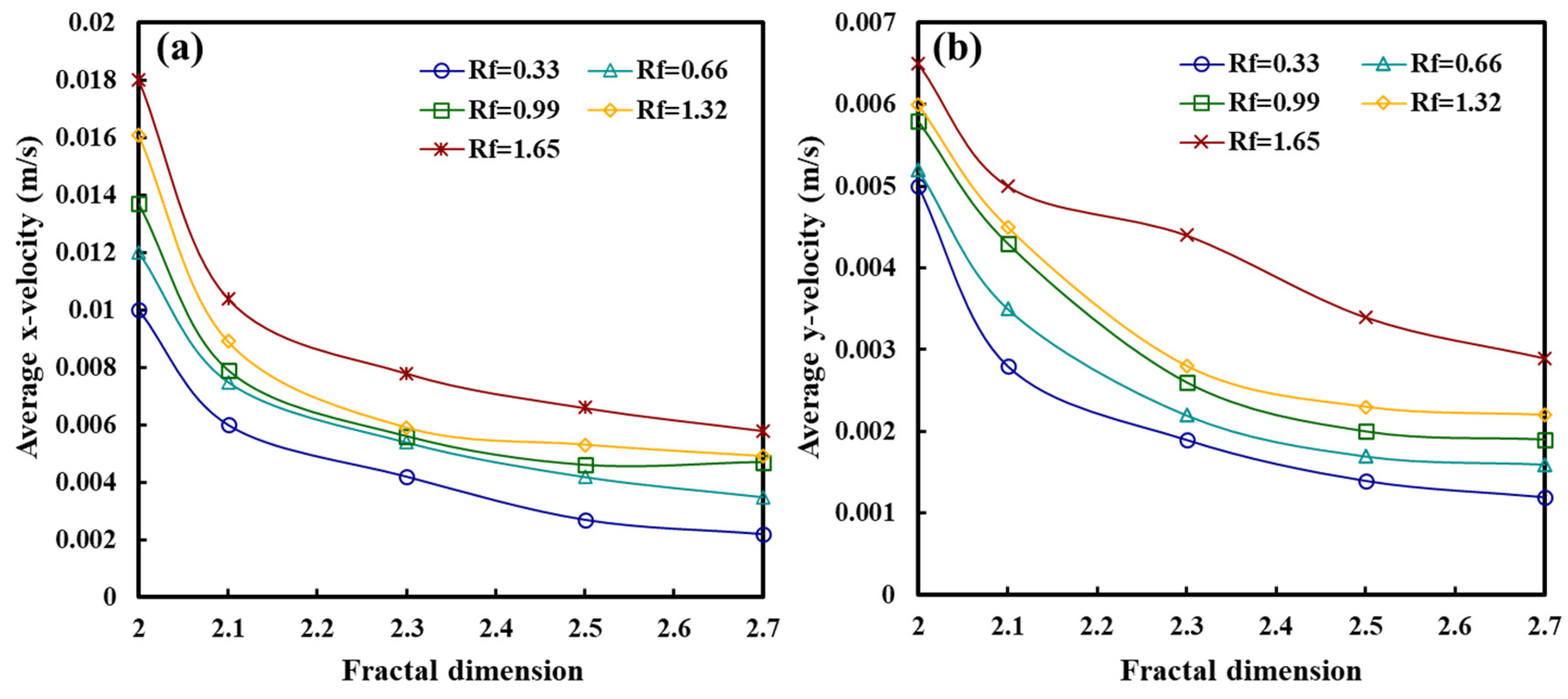
4.2. Effect of the Ratio of Lateral to Longitudinal Forces on the Proppant (R_f)

In this section, we study the effect of the ratio of lateral and longitudinal forces on the transport and distribution of the proppant. In the slurry, the movement of the proppant is influenced by various forces, including buoyancy, gravity, viscous resistance, and inertia. In this study, the Reynolds number of the fluid during the proppant injection process is approximately 600. This value indicates that the flow within the fracture is mainly in a laminar state. And the particle Reynolds number is very low, indicating that the movement of the proppant in the fluid is mainly affected by viscous forces. The calculation of the drag force experienced by the proppant is typically based on Stokes’ Law

$$F_g=3\pi \mu du$$

(11)

where $F_g$ is the drag force of the proppant; $\mu$ is the viscosity of the fluid; $d$ is the diameter of the proppant; and $u$ is the relative velocity of the proppant. In the study of proppant motion in fluids, two principal factors influence the behavior of the proppant: the drag force exerted laterally and the gravitational and buoyancy forces exerted longitudinally. Therefore, we define the ratio of the forces on the proppant laterally to those longitudinally as a dimensionless number (R_f). R_f is calculated as follows:

$$R_f={\displaystyle \frac{18\mu u_x}{\left({\rho }_p-{\rho }_f\right)d^{2}g-18\mu u_y}}$$

(12)

where ${\rho }_p$ is the density of the proppant;${\rho }_f$ is the density of the fluid; and $g$ is the acceleration due to gravity.

Figure 10 compares the morphology of the proppant dunes in rough fractures after 10 s of injection, with varying fractal dimensions and R_f. It is seen that an increase in R_f can significantly enhance the fluid’s proppant-carrying capacity and extend the lateral transport distance of the proppant. As R_f is less than 0.99, the dunes show a typical triangular shape. As R_f increases to 1.32, the morphology of the dune gradually shifts to a flatter, trapezoidal shape, and the height of the dune decreases.

We further analyze the relationship between the average proppant transport distance and the fractal dimension. As shown in Figure 11a, when the R_f value is less than 0.99, the average x-coordinate decreases as the fractal dimension rises. When the R_f value exceeds 0.99, the average x-coordinate is trivially influenced by the fractal dimension. The proppant is observed to be more concentrated in the central region of the fracture in Figure 9. Figure 11b illustrates that the average y-coordinate increases with the fractal dimension. Conversely, the y-coordinate decreases with an increase in the R_f value.

To quantify the effect of roughness on proppant transport, we analyzed the transverse and longitudinal velocities of the proppant in fractures of different fractal dimensions. Figure 12a illustrates that the average x-velocity decreases as the fractal dimension increases. It is noted that in Figure 11b, the average y-velocity of the proppant is low in fractures with high fractal dimensions. Additionally, as the R_f value increases, both the average x- and y-velocity increase. The main reason for this phenomenon is that as the R_f value increases, the resistance experienced by the proppant in the direction of gravity also increases, which enables them to remain suspended for longer periods.

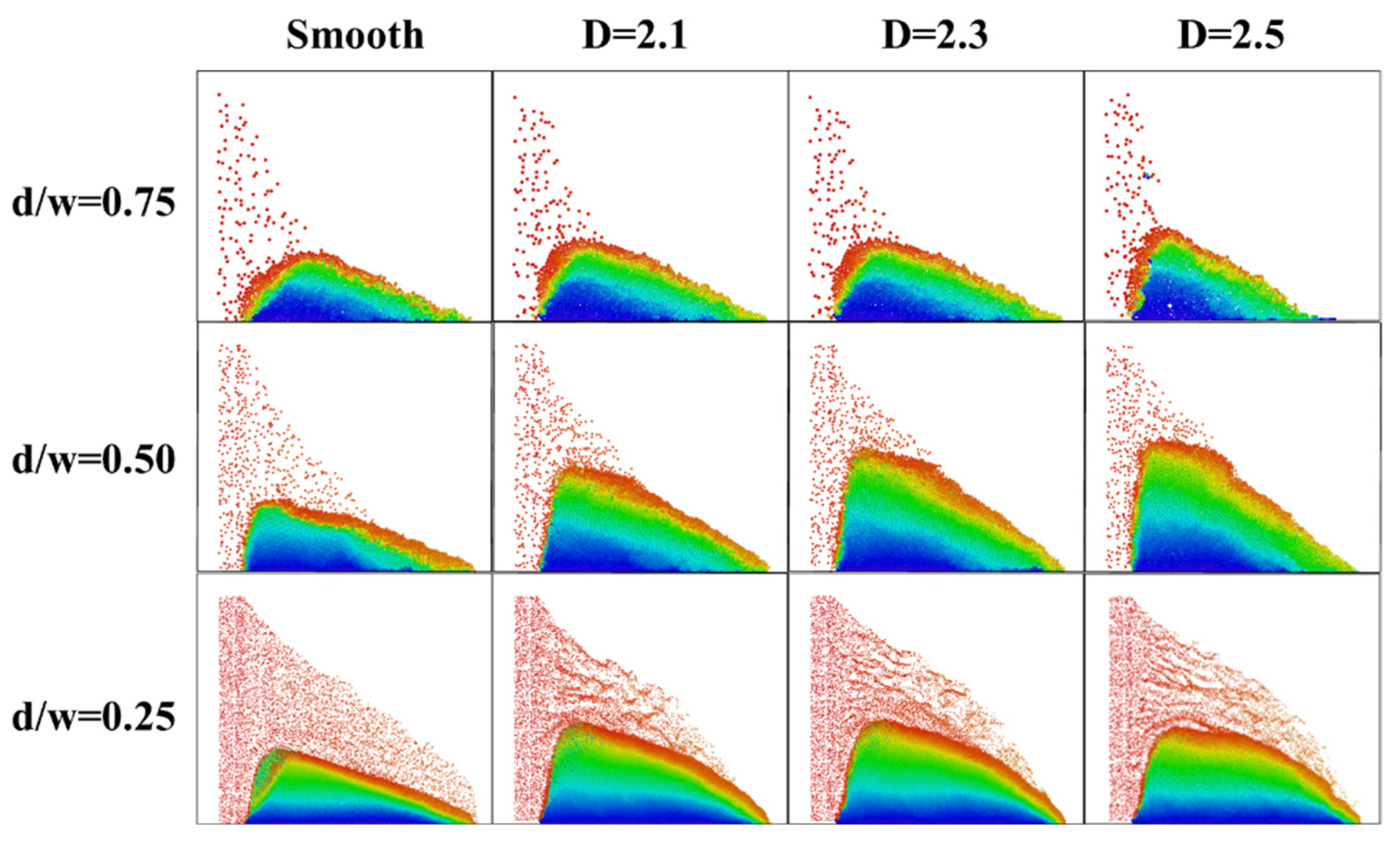
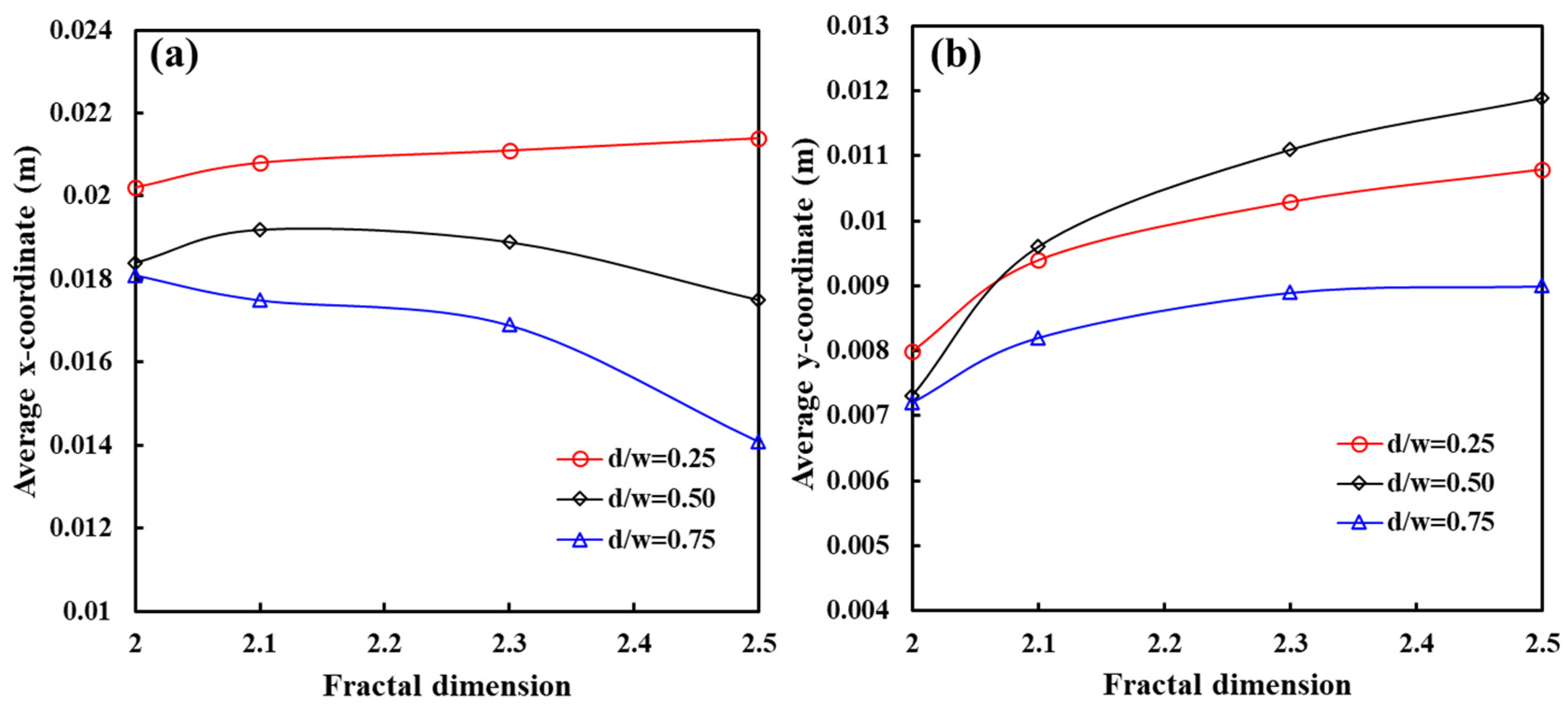
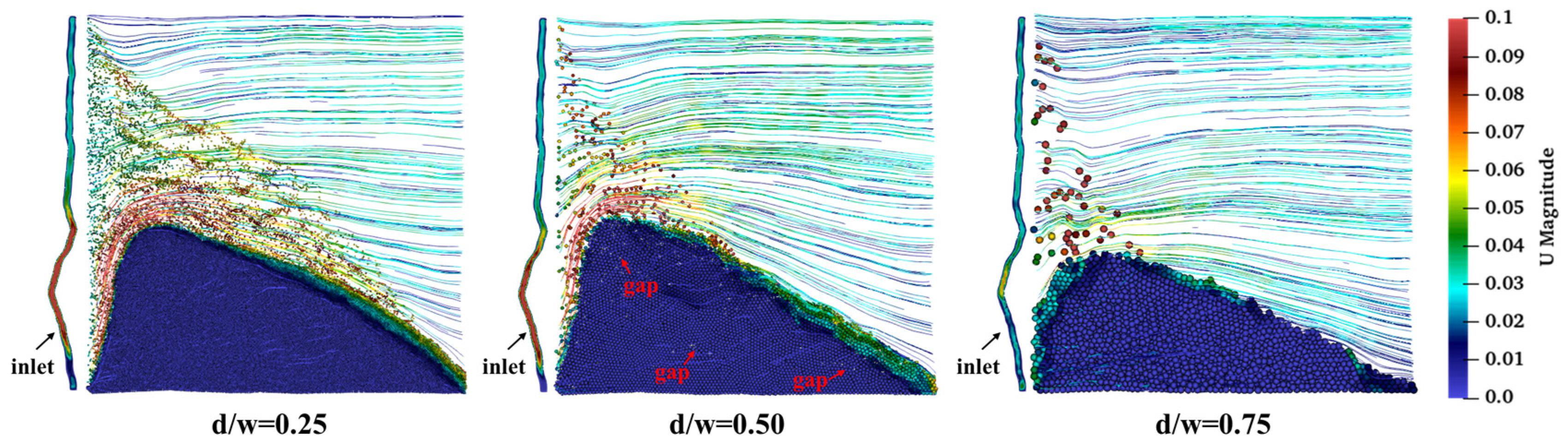
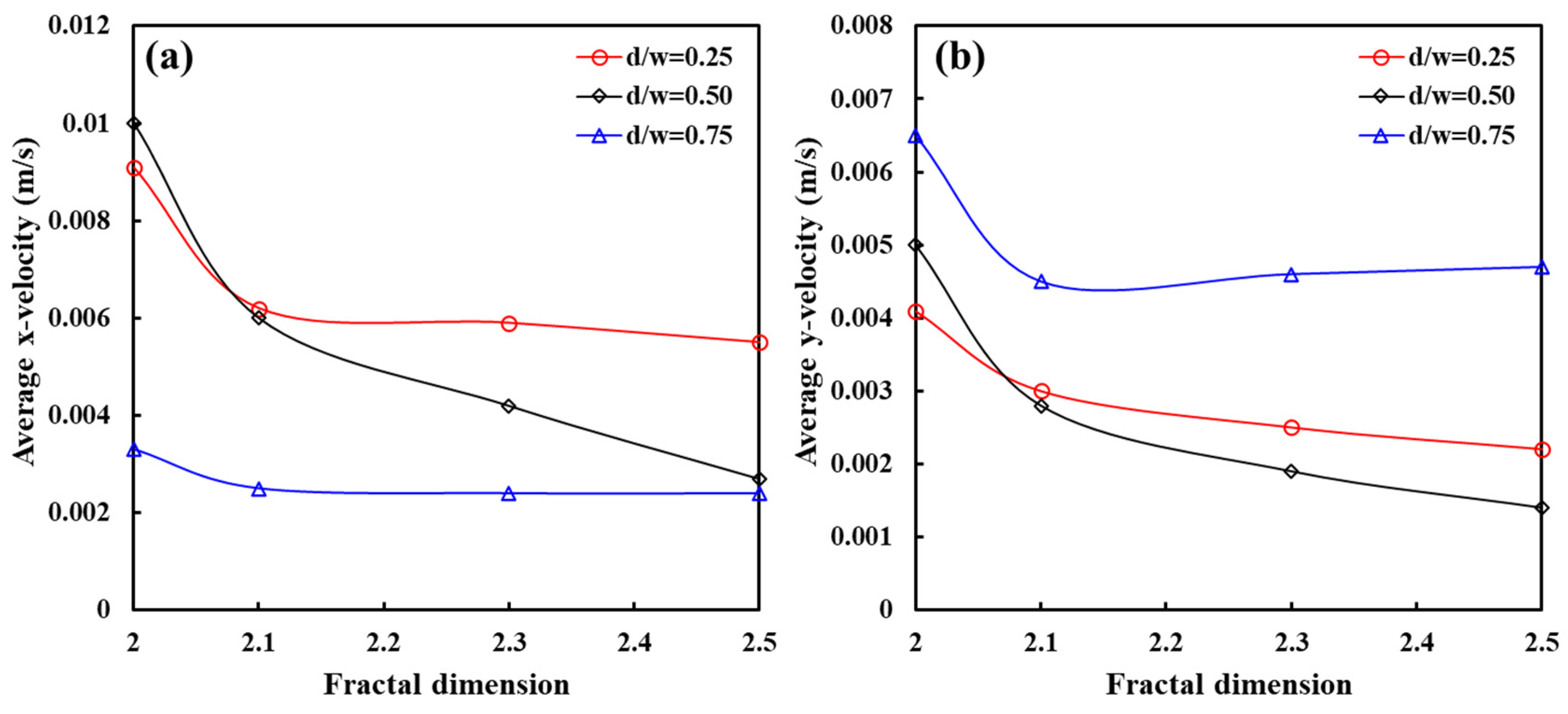
4.3. Effect of the Ratio of the Proppant Diameter to the Fracture Aperture (d/w)

The ratio of the proppant diameter to the fracture aperture is also a critical factor affecting the proppant transport. As the fractal dimension of the fracture increases, there is a higher probability and frequency of particle collisions with the fracture wall, resulting in diminished proppant transport. A shown in Figure 13, it is observed that when the d/w value is 0.25, the effect of roughness on proppant transport is trivial. The final dune heights are gradually equilibrium in fractures with different roughness. Upon increasing the d/w value to 0.75, the area covered by dunes within the fractures is significantly reduced at d/w values of 0.25 and 0.5. And a notable impediment to proppant transport was observed.

We further analyze the relationship between the fractal dimension and the position of the proppant. According to Figure 14a, when the d/w value is 0.25, the average x-coordinate is approximately equilibrium for different fractal dimensions. As the d/w value exceeds 0.25, the increased roughness causes the average x-coordinate to decrease. It is evident from Figure 14b that the average y-coordinate at the d/w ratio of 0.25 is lower than the average y-coordinate at a d/w ratio of 0.50. This phenomenon can be explained by Figure 15, which shows that fractures at a d/w ratio of 0.5 exhibit both a high fill rate and a significant number of gaps.

We further analyzed the interactions between the fluid and the proppant at different d/w values and the impact of roughness on the proppant across these values. Figure 15 illustrates streamlines and proppant velocities in a rough fracture with a fractal dimension of 2.1. As the d/w value increases, the area covered by the suspended proppant in the fracture decreases, and the proppant is transported a shorter distance. Additionally, as the d/w value increases, the frequency of particle collisions with the fracture wall increases, which consequently decreases the transport velocity of the proppant. This size effect is particularly evident with the high d/w value, as proppants are more likely to be obstructed by the fracture walls. Observing the cloud map of the fluid velocity at the injection surface, we found that in the central region of the fracture, the transport velocity of the proppant reaches a maximum due to wall shear action and increased local flow velocity. Conversely, the flow velocity decreases near the fracture wall, resulting in a slower proppant transport velocity. This indicates that with a smaller d/w value, the proppant in the central region of the fracture can penetrate more deeply into the fracture, thereby expanding the recovery area.

To observe the effect of roughness on proppant transport more intuitively, we analyzed the average x- and y-velocities of the proppant for different d/w values. As illustrated in Figure 16a, the average x-velocity decreases with an increasing fractal dimension, particularly noticeable at a d/w ratio of 0.5, while it remains relatively equilibrium at d/w ratios of 0.25 and 0.75. Furthermore, as the d/w value increases, the average x-velocity decreases, indicating that rough fractures exert a greater influence on particle transport at higher d/w values. Figure 16b shows that the average y-velocity decreases as the fractal dimension increases for d/w ratios of 0.5 and 0.25, and remains equilibrium for a d/w ratio of 0.75. Notably, the average y-velocity at a d/w ratio of 0.5 is less than that at a d/w ratio of 0.25. This indicates that a higher settling velocity of proppant does not necessarily mean that the proppant will settle more easily.

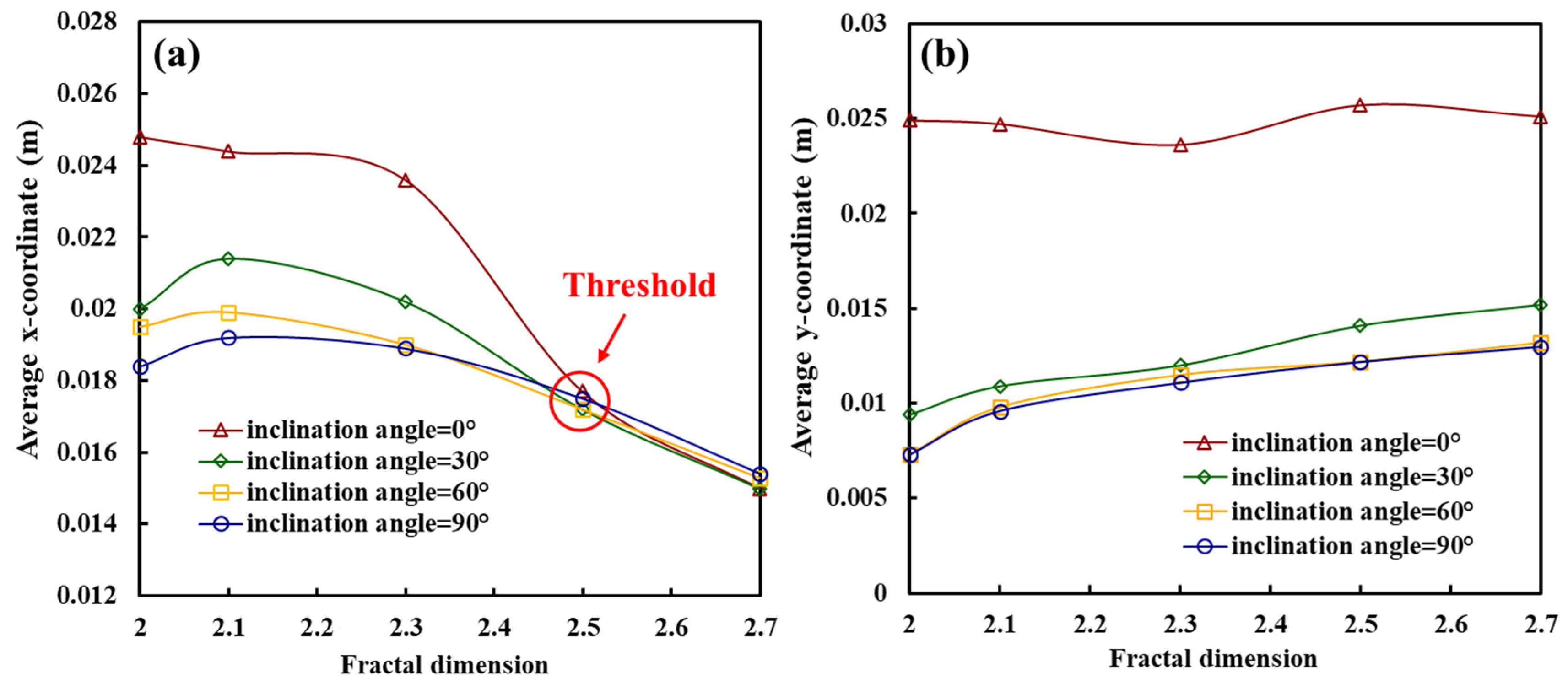
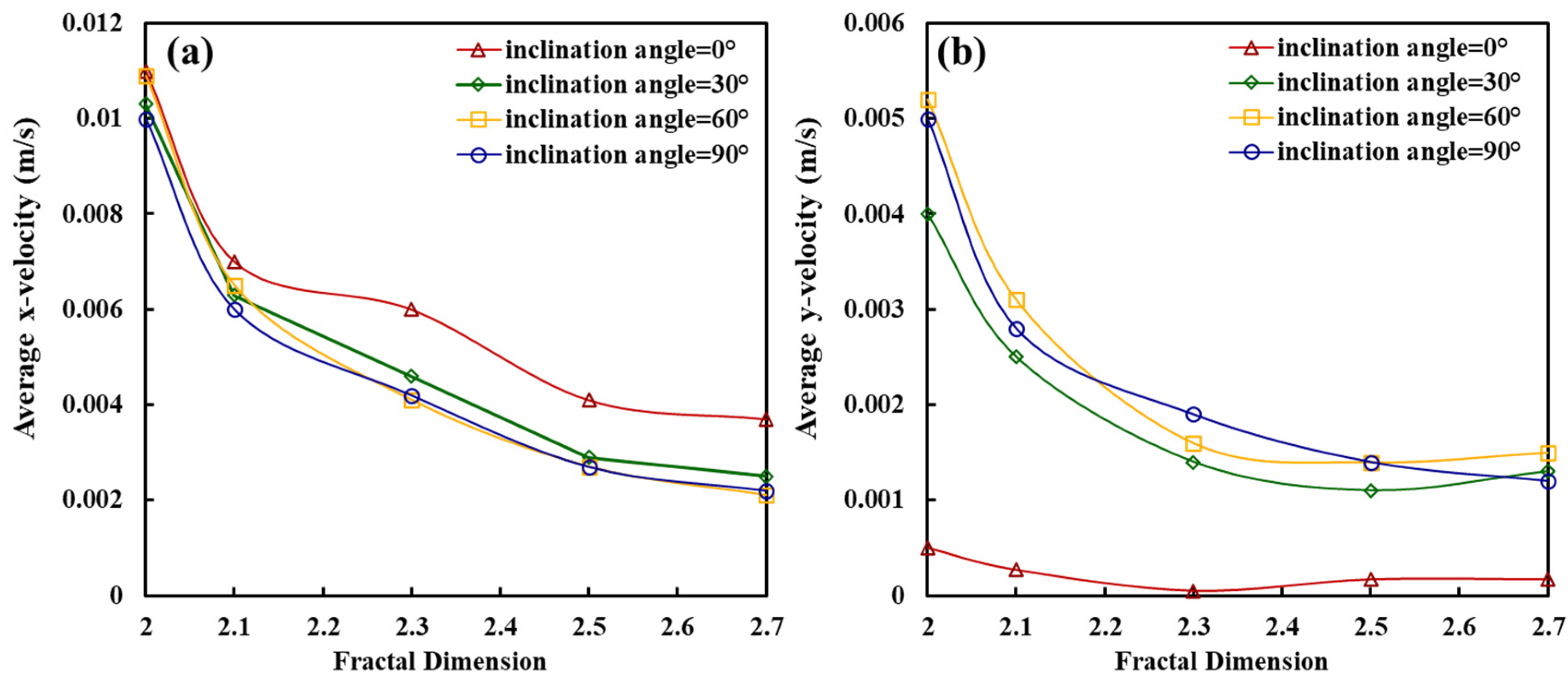
4.4. Effect of Inclination Angle at Different Fracture Dimensions

The inclination angle of fractures has a significant effect on the transport of the proppant [47]. Within inclined fractures, the gravitational settling of the proppant is partially offset by contact with the surface, allowing for more lateral transport distance for the proppant. In unconventional reservoirs, preexisting natural fractures, including a significant number of inclined and even horizontal fractures, have been observed during hydraulic fracturing. Field studies have shown that hydraulic fractures are rarely vertical and that the orientation changes with the distance from the wellbore [48,49,50]. In this section, we explore proppant transport and distribution with different inclination angles.

Figure 17 illustrates the impact of the inclination angles on the areas and morphologies of sand dunes. In horizontal fractures, the sedimentation space is limited, thus reducing the impact of gravity. The friction force reaches its maximum value on the horizontal plane, facilitating the uniform distribution of piston-like sand clusters. Consequently, the fluid plays a more significant role in the distribution of the proppant than gravity, with lateral migration becoming the primary factor. The horizontal expansion of the sand dune is mainly driven by rolling rather than direct sedimentation. The roughness of the fracture significantly affects the distribution of the proppant, as the fractal dimension increases, reducing the lateral transport distance of the proppant. When the inclination angle is 30° and 60°, the sedimentation rate of the proppant accelerates, leading to the formation of sand dunes near the injection surface. At 30°, the proppant is more likely to form bridging, where more sand clusters can be observed. This is beneficial for enhancing the fracture permeability and increasing the flow capacity. As the fractal dimension increases, the undulations of the fracture surface become more pronounced, and the number of sand clusters increases. At 60°, the proppant tends to deposit at the bottom of the fracture, with a significant reduction in the bridging effect. Moreover, the lateral transport distance of the proppant at 60° is greater than at 90°. This indicates that as the inclination angle decreases, the friction force between the proppant and fracture walls increases, thereby enabling the proppant to be transported farther. The lower inclination angle also means that the proppant tends to transport in the lateral, which helps to cover a wider area.

We further analyze the relationship between the average proppant transport distance and the fractal dimension. Figure 18 demonstrates the effect of fracture inclination angles on the average x- and y-coordinates. When the fractal dimension is less than 2.5, there is a corresponding decrease in the lateral transport distance with an increase in the fractal dimension. Conversely, once the fractal dimension surpasses the threshold of 2.5, the influence of the inclination angle on the transport of the proppant becomes minimal.

In Figure 19, the average x- and y-velocities of the proppant with different inclination angles decreases with an increasing fractal dimension. Velocity differences within both inclined and horizontal fractures are significant, primarily due to variations in fracture roughness. When comparing inclined fractures with different fractal dimensions, the average x-velocity decreases and the average y-velocity increases as the inclination angle increases.

We compare the velocity of the proppant and the streamlines of fluid to analyze the change in dune shapes with different fractal dimensions. As shown in Figure 20, taking the fracture with 30° as an example, the presence of sand clusters appears to encourage the proppant to move toward the upper part of the fracture at fractal dimensions of 2.1 and 2.5. If the proppant becomes concentrated at the bottom of the fracture, it could potentially cause the upper part to close, which would significantly reduce the fracture conductivity. The aggregation of the proppant into clusters is beneficial as it enhances fracture support and contributes to the creation of fractures with a greater flow capacity.

5. Conclusions

Hydraulic fracturing plays a crucial role in the development of offshore unconventional reservoirs. In summary, most current research has primarily focused on the longitudinal or transverse roughness of fractures, failing to capture the three-dimensional characteristics and not fully simulating the complex morphology of the fracture surface. In this work, we conduct a quantitative analysis of the transport and distribution of the proppant in rough fractures with varying fractal dimensions using the CFD-DEM approach, with the results validated against experimental data. It is found that increased fracture roughness significantly reduces the proppant transport efficiency, reduces the lateral transport distance, and causes the proppant to accumulate near the injection surface. After the dune height reaches equilibrium, the proppant will be transported at a relatively constant rate, and transport behavior is dominated by rolling. We further analyze the influence of the main-control factors on the proppant transport in rough fractures. Our findings indicate that an increase in the ratio of lateral to longitudinal forces on the proppant significantly reduces the settling velocity and enhances its lateral transport efficiency. When the ratio is low, fracture roughness significantly affects the lateral transport of the proppant. Conversely, at high ratios, the effects become negligible. As the proppant size increases, there is increased dependence of the proppant movement and deposition on the fracture aperture. Proppant transport in rough fracture is more hindered by an increase in the ratio of the proppant diameter to fracture aperture, particularly when the ratio exceeds 0.5. Furthermore, when the fractal dimension is below 2.5, the lateral transport distance of the proppant tends to decrease with an increasing inclination angle. Once the fractal dimension exceeds 2.5, the influence of the inclination angle on the transport of the proppant is negligible. As the fracture inclination decreases, the lateral transport of the proppant also decreases. The proppant migrates along the fracture surface and predominantly accumulates in depressions. This phenomenon, known as “bridging,” leads to enhanced accumulation of the proppant and the formation of sand clusters. Our research, particularly the computational simulation of proppant transport in 3D rough fractures, establishes a reference point for estimating proppant distribution.

References

1. Mayerhofer, M.; Lolon, E.; Warpinski, N. What is stimulated reservoir volume? SPE Prod. Oper. 2010, 25, 89–98. [Google Scholar] [CrossRef]
2. Daneshy, A. Hydraulic fracturing to improve production. Way Ahead 2010, 6, 14–17. [Google Scholar] [CrossRef]
3. Guo, X.; Hu, D.; Li, Y. Theoretical progress and key technologies of onshore ultra-deep oil/gas exploration. Engineering 2019, 5, 458–470. [Google Scholar] [CrossRef]
4. Miller, C.; Waters, G.; Ryalander, E. Evaluation of production log data from horizontal wells drilled in organic shales. In Proceedings of the North American Unconventional Gas Conference and Exhibition, The Woodlands, TX, USA, 14–16 June 2011. Paper SPE-144326-MS. [Google Scholar]
5. Zhao, J.; Ren, L.; Jiang, T. Ten years of gas shale fracturing in China: Review and prospect. Nat. Gas Ind. B 2022, 9, 158–175. [Google Scholar] [CrossRef]
6. Ma, X.; Wang, H.; Zhang, Q. “Extreme utilization” development of deep shale gas in southern Sichuan Basin, SW China. Pet. Explor. Dev. 2022, 49, 1377–1385. [Google Scholar] [CrossRef]
7. Aydin, A.; Schultz, R. Effect of mechanical interaction on the development of strike-slip faults with echelon patterns. J. Struct. Geol. 1990, 12, 123–129. [Google Scholar] [CrossRef]
8. Babadagli, T.; Develi, K. Fractal characteristics of rocks fractured under tension. Theor. Appl. Fract. Mech. 2003, 39, 73–88. [Google Scholar] [CrossRef]
9. Zhang, Y.; Chai, J. Effect of surface morphology on fluid flow in rough fractures: A review. J. Nat. Gas Sci. Eng. 2020, 79, 103343. [Google Scholar] [CrossRef]
10. Zhu, G.; Zhao, Y.; Zhang, T. Micro-scale reconstruction and CFD-DEM simulation of proppant-laden flow in hydraulic fractures. Fuel 2023, 352, 129151. [Google Scholar] [CrossRef]
11. Siddhamshetty, P.; Wu, K.; Kwon, J. Modeling and control of proppant distribution of multistage hydraulic fracturing in horizontal shale wells. Ind. Eng. Chem. Res. 2019, 58, 3159–3169. [Google Scholar] [CrossRef]
12. Raimbay, A.; Babadagli, T.; Kuru, E. Quantitative and visual analysis of proppant transport in rough fractures. J. Nat. Gas Sci. Eng. 2016, 33, 1291–1307. [Google Scholar] [CrossRef]
13. Huang, H.; Babadagli, T.; Li, H. A visual experimental study on proppants transport in rough vertical fractures. Int. J. Rock Mech. Min. Sci. 2020, 134, 104446. [Google Scholar] [CrossRef]
14. Gong, F.; Huang, H.; Babadagli, T. A computational model to simulate proppant transport and placement in rough fractures. In Proceedings of the SPE Hydraulic Fracturing Technology Conference and Exhibition, The Woodlands, TX, USA, 1–3 February 2022. p. D021S003R006.
15. Huang, F.; Wang, F.; Chen, F. Transport and Retention of Coal Fines in Proppant Packs during Gas–Water Two–Phase Flow: Insights from Interface, Pore, to Laboratory Scales. Energy Fuels 2024, 38, 12672–12683. [Google Scholar] [CrossRef]
16. Ranjith, P.G.; Viete, D.R. Applicability of the ‘cubic law’ for non-Darcian fracture flow. J. Pet. Sci. Eng. 2011, 78, 321–327. [Google Scholar] [CrossRef]
17. Chen, Y.; Liang, W.; Lian, H.; Yang, J.; Nguyen, V.P. Experimental study on the effect of fracture geometric characteristics on the permeability in deformable rough-walled fractures. Int. J. Rock Mech. Min. Sci. 2017, 98, 121–140. [Google Scholar] [CrossRef]
18. Wang, L.; Cardenas, M.B.; Slottke, D.T.; Ketcham, R.A.; Sharp, J.M., Jr. Modification of the Local Cubic Law of fracture flow for weak inertia, tortuosity, and roughness. Water Resour. Res. 2015, 51, 2064–2080. [Google Scholar] [CrossRef]
19. Yin, Q.; Ma, G.; Jing, H.; Wang, H.; Su, H.; Wang, Y.; Liu, R. Hydraulic properties of 3D rough-walled fractures during shearing: An experimental study. J. Hydrol. 2017, 555, 169–184. [Google Scholar] [CrossRef]
20. Xie, J.; Hu, Y.; Kang, Y. Numerical study on proppant transport in supercritical carbon dioxide under different fracture shapes: Flat, wedge-shaped, and bifurcated. Energy Fuels 2022, 36, 10278–10290. [Google Scholar] [CrossRef]
21. Zhou, M.; Yang, Z.; Xu, Z. CFD-DEM modeling and analysis study of proppant transport in rough fracture. Powder Technol. 2024, 436, 119461. [Google Scholar] [CrossRef]
22. Cao, C.; Xu, Z.; Chai, J.; Qin, Y.; Tan, R. Mechanical and hydraulic behaviors in a single fracture with asperities crushed during shear. Int. J. Geomech. 2018, 18, 04018148. [Google Scholar] [CrossRef]
23. Lee, J.; Kang, J.M.; Choe, J. Experimental analysis on the effects of variable apertures on tracer transport. Water Resour. Res. 2003, 39. [Google Scholar] [CrossRef]
24. Huang, N.; Liu, R.; Jiang, Y. Numerical study of the geometrical and hydraulic characteristics of 3D self–affine rough fractures during shear. J. Nat. Gas Sci. Eng. 2017, 45, 127–142. [Google Scholar] [CrossRef]
25. Xie, L.Z.; Gao, C.; Ren, L.; Li, C.B. Numerical investigation of geometrical and hydraulic properties in a single rock fracture during shear displacement with the Navier–Stokes equations. Environ. Earth Sci. 2015, 73, 7061–7074. [Google Scholar] [CrossRef]
26. Suri, Y.; Islam, S.; Hossain, M. Effect of fracture roughness on the hydrodynamics of proppant transport in hydraulic fractures. J. Nat. Gas Sci. Eng. 2020, 80, 103401. [Google Scholar] [CrossRef]
27. Zhang, M.; Wu, C.; Sharma, M. Proppant placement in perforation clusters in deviated wellbores. In Proceedings of the Unconventional Resources Technology Conference, Denver, Colorado, 22–24 July 2019; p. D013S014R002, SPE/AAPG/SEG. [Google Scholar]
28. Zhang, B.; Gamage, R.; Zhang, C. Hydrocarbon recovery: Optimized CFD-DEM modeling of proppant transport in rough rock fractures. Fuel 2022, 311, 122560. [Google Scholar] [CrossRef]
29. Guo, T.; Luo, Z.; Zhou, J. Numerical simulation on proppant migration and placement within the rough and complex fractures. Pet. Sci. 2022, 19, 2268–2283. [Google Scholar] [CrossRef]
30. Gong, Z.; Li, N.; Kang, W. Novel oleophilic tracer-slow-released proppant for monitoring the oil production contribution. Fuel 2024, 364, 130945. [Google Scholar] [CrossRef]
31. Hu, X.; Wu, K.; Li, G. Effect of proppant addition schedule on the proppant distribution in a straight fracture for slickwater treatment. J. Pet. Sci. Eng. 2018, 167, 110–119. [Google Scholar] [CrossRef]
32. Zhou, Z.; Shen, L.; Wang, J. Numerical investigating the effect of nonuniform proppant distribution and unpropped fractures on well performance in a tight reservoir. J. Pet. Sci. Eng. 2019, 177, 634–649. [Google Scholar] [CrossRef]
33. Movassagh, A.; Haghighi, M.; Zhang, X. A fractal approach for surface roughness analysis of laboratory hydraulic fracture. J. Nat. Gas Sci. Eng. 2021, 85, 103703. [Google Scholar] [CrossRef]
34. Xie, H.; Sun, H.; Ju, Y. Study on generation of rock fracture surfaces by using fractal interpolation. Int. J. Solids Struct. 2001, 38, 5765–5787. [Google Scholar] [CrossRef]
35. Issa, M.; Islam, M. Fractal dimension––A measure of fracture roughness and toughness of concrete. Eng. Fract. Mech. 2003, 70, 125–137. [Google Scholar] [CrossRef]
36. Charkaluk, E.; Bigerelle, M.; Iost, A. Fractals and fracture. Eng. Fract. Mech. 1998, 61, 119–139. [Google Scholar] [CrossRef]
37. Babadagli, T.; Develi, K. On the application of methods used to calculate the fractal dimension of fracture surfaces. Fractals 2001, 9, 105–128. [Google Scholar] [CrossRef]
38. Kloss, C.; Goniva, C.; Hager, A. Models, algorithms and validation for opensource DEM and CFD–DEM. Prog. Comput. Fluid Dyn. Int. J. 2012, 12, 140–152. [Google Scholar] [CrossRef]
39. Weller, O.; Lange, D.; Tilmann, F. The structure of the Sumatran Fault revealed by local seismicity. Geophys. Res. Lett. 2012, 39, 1–7. [Google Scholar] [CrossRef]
40. Hertz, H. Über die Berührung fester elastischer Körper. J. Reine Und Angew. Math. 1881, 92, 156. [Google Scholar]
41. Mindlin, R.; Deresiewicz, H. Elastic spheres in contact under varying oblique forces. J. Appl. Mech. Sep. 1953, 20, 327–344. [Google Scholar] [CrossRef]
42. Felice, R.D. The void age function for fluid-particle interaction systems. Int. J. Multiph. Flow 1994, 20, 153–159. [Google Scholar] [CrossRef]
43. Tong, S.; Mohanty, K.K. Proppant transport study in fractures with intersections. Fuel 2016, 181, 463–477. [Google Scholar] [CrossRef]
44. Isakov, E.; Ogilvie, S.; Taylor, C. Fluid flow through rough fractures in rocks I: High resolution aperture determinations. Earth Planet. Sci. Lett. 2001, 191, 267–282. [Google Scholar] [CrossRef]
45. Ogilvie, G. On the dynamics of magneto rotational turbulent stresses. Mon. Not. R. Astron. Soc. 2003, 340, 969–982. [Google Scholar] [CrossRef]
46. Xie, J.; Gao, M.; Zhang, R. Experimental investigation on the anisotropic fractal characteristics of the rock fracture surface and its application on the fluid flow description. J. Pet. Sci. Eng. 2020, 191, 107190. [Google Scholar] [CrossRef]
47. Chun, T.; Li, Y.; Wu, K. Comprehensive experimental study of proppant transport in an inclined fracture. J. Pet. Sci. Eng. 2020, 184, 106523. [Google Scholar] [CrossRef]
48. Daneshy, A. A study of inclined hydraulic fractures. Soc. Pet. Eng. J. 1973, 13, 61–68. [Google Scholar] [CrossRef]
49. Agrawal, G.; Kumar, A.; Dutta, S. Productivity Optimization and Validation of Multistage Fracturing in a Rare et al. Geomechanical Setting with Production Logging. In Proceedings of the Offshore Technology Conference, Houston, TX, USA, 16–19 August 2021; p. D021S028R006. [Google Scholar]
50. Kumar, A.; Sharma, M. Diagnosing hydraulic fracture geometry, complexity, and fracture wellbore connectivity using chemical tracer flowback. Energies 2020, 13, 5644. [Google Scholar] [CrossRef]
Figure 1. The change in surface morphology with an increasing fractal dimension.
Jmse 12 02117 g001
Figure 2. (a) Comparison of the simulation and experiment proppant placement at different times. (b) Comparison between the experimental data and the simulation results for the sand dune height. (c) Comparison between the experimental data and the simulation results for the sand dune length.
Jmse 12 02117 g002
Figure 3. 3D rough fracture with different fractal dimensions.
Jmse 12 02117 g003
Figure 4. (a) Schematic of initial and boundary conditions. (b) Four sets of inclination angles. (c) Mesh distribution of rough fracture with a fractal dimension of 2.1 in the simulation. (d) Mesh resolution analysis in the simulation.
Jmse 12 02117 g004
Figure 5. Comparison of proppant dune generation processes in vertical rough fractures with different fractal dimensions.
Jmse 12 02117 g005
Figure 6. (a) The process of changing the length of sand dunes with different fractal dimensions. (b) The process of changing the height of sand dunes with different fractal dimensions.
Jmse 12 02117 g006
Figure 7. (a) The height of the dunes with different varying fractal dimensions at 10 s. (b) The average x- and y-coordinate of all proppants with different fractal dimensions at 10 s.
Jmse 12 02117 g007
Figure 8. (a) Average x-velocities of the proppant with different fractal dimensions in the injection direction at 10 s. (b) Average y-velocities of the proppant with different fractal dimensions at 10 s.
Jmse 12 02117 g008
Figure 9. Fluid streamlines with different fractal dimensions at 10 s.
Jmse 12 02117 g009
Figure 10. Comparison of proppant dune morphology in rough fracture at 10 s equilibrium for different fractal dimensions and Rf.
Jmse 12 02117 g010
Figure 11. (a) Average x-coordinate of all proppants at 10 s equilibrium for different fractal dimensions and Rf. (b) Average y-coordinate of all proppants at 10 s equilibrium for different fractal dimensions and Rf.
Jmse 12 02117 g011
Figure 12. (a) Average x-velocity of the proppant at 10 s with different fractal dimensions and Rf. (b) Average y-velocity of the proppant at 10 s with different fractal dimensions and Rf.
Jmse 12 02117 g012
Figure 13. Comparison of proppant dune morphology with different fractal dimensions and d/w at 10 s.
Jmse 12 02117 g013
Figure 14. (a) Average x-coordinate of all proppants with different d/w at 10 s. (b) Average y-coordinate of all proppants with different d/w at 10 s.
Jmse 12 02117 g014
Figure 15. Fluid streamlines in a rough fracture with a fractal dimension of 2.1 and different d/w at 10 s.
Jmse 12 02117 g015
Figure 16. (a) Average x-velocity of all proppants with different fractal dimensions and d/w at 10 s. (b) Average y-velocity of all proppants with different fractal dimensions and d/w at 10 s.
Jmse 12 02117 g016
Figure 17. Comparison of a proppant dune in rough fracture with different fractal dimensions and inclination angles at 10 s.
Jmse 12 02117 g017
Figure 18. (a) Average x-coordinate of the proppant with different fractal dimensions and inclination angles at 10 s. (b) Average y-coordinate of the proppant with different fractal dimensions and inclination angles at 10 s.
Jmse 12 02117 g018
Figure 19. (a) Average x-velocity of all proppants with different fractal dimensions and inclination angles at 10 s. (b) Average y-velocity of all proppants with different fractal dimensions and inclination angles at 10 s.
Jmse 12 02117 g019
Figure 20. Fluid streamlines in 30° with different fractal dimensions at 10 s.
Jmse 12 02117 g020