Abstract
Vehicles travelling underwater experience drag and the frictional drag costs 60% of the total energy consumption. Using trapped air serving as a lubricant is a promising way to reduce drag. The trapped air plays a significant role in drag reduction, and most failures in drag reduction are related to instability, escape, and dissolution of the trapped air. In this work, discrete grooves are employed to trap air and reduce drag. Through the analysis of the trapped air stability, the groove length and width are believed to be the main factors that influence the air escape and instability, and thus they are limited in this work to avoid these problems. The air dissolution is inevitable. The effective way to mitigate the air dissolution is to deepen the groove depth. The groove depth in this work varies from 0.5 mm to 4 mm. The numerical simulation is employed to analyze the flow field, reveal the drag reduction mechanism, and optimize the groove length. The experimental measurements are conducted to verify our design. The result confirms our design that the discrete grooves successfully avoid air escape and instability, mitigate air dissolution, and reduce drag. This work is meaningful for underwater vehicles to travel with low energy consumption and high speed.
1. Introduction
Vehicles travelling underwater experience pressure drag and frictional drag. The pressure drag comes from the pressure difference around the vehicles and is related to the vehicle’s appearance. Nowadays, the vehicle appearance is streamlined enough and the remained space for reducing the pressure drag is small. The ideal choice is reducing the frictional drag. Ways for reducing frictional drag include boundary layer control and slippery surfaces. Ways for the boundary layer control include riblet surfaces [1,2], vibrating surfaces [3,4] and polymer additives [5,6]. The slippery surfaces include air-lubricant surfaces [7,8] and liquid-infused surfaces [9,10]. The air-lubricant surface uses trapped air serving as the lubricant and is reported to reach a drag reduction rate of 75% [11]. The excellent drag reduction rate of the air-lubricant surface makes this method attractive and promising.
The slippery trapped air is the main cause of the drag reduction. The trapped air morphology has a strong effect on the drag reduction rate. As one can imagine, the drag reduction rate should be proportional to the trapped air coverage rate. Park et al. [11] examined the drag reduction rate at different trapped air coverage rates and the result showed that the drag reduction rate increased when the trapped air coverage rate increased. The best drag reduction rate of 75% was obtained at the trapped air coverage rate of approximately 97%. When the trapped air escapes or vanishes from the surface, the drag reduction rate decreases. Reholon and Ghaemi [12] recorded the trapped air morphology and analyzed its relationship with the drag reduction rate. Their results showed that the drag reduction rate decreased when the trapped air gradually dissolved into the water. The results of Xu et al. [8] showed a similar relationship between the trapped air morphology and the drag reduction rate. These works indicate that attention should be paid to the trapped air stability.
In the drag reduction application of air-lubricant surface, problems such as air instability, escape, and dissolution are met. For the ventilating surface, the air layer is supplied by a ventilating system at the leading edge of the surface and a large downward cavity is used to trap air. The common problems for the ventilating surface are that the trapped air fluctuates or sheds. Lay et al. [13] reported air instability and shedding for the ventilating surface. They reported that the shedding frequency is proportional to the cavity dimensions. Mäkiharju et al. [14] reported that the fluctuation and shedding of the trapped air were as large as the order of 10 cm. They also reported that the required air flux to maintain the trapped air layer increased with the increasing Weber number. Hao et al. [15] reported that deep cavity could prevent the air escape and thus enhance the drag reduction performance. For the large cavity, the capillary force is weak and the air is mainly trapped by flotation. Small surface textures produce large capillary force and thus prevent the trapped air instability and shedding [16,17,18]. For the superhydrophobic surface, the air is trapped in the surface microcavities by the capillary force. The trapped air instability and shedding are avoided. However, a common problem for the superhydrophobic surface is that the trapped air escapes or dissolves. Through our review of the existing works, the dissolution of the trapped air seems to be the main problem. In the work of Aljallis et al. [19], they suspected that the trapped air in the superhydrophobic microcavities was removed by the flowing water. The work of Xu et al. [8] showed that the trapped air in the superhydrophobic microgrooves escaped during the towing tank experiment. The work of Kim and Hidrovo [20] reported that the trapped air in microgrooves dissolved into water automatically. The work of Lv et al. [21] showed that the trapped air in microgrooves would totally dissolve into the water in 30 min at a low pressure of 14 kPa (relative to the barometric pressure). The work of Ling et al. [22] showed that the flowing water accelerated the dissolution process. Reholon and Ghaemi [12] reported that trapped air in the surface microcavities dissolved in water when they were trying to obtain drag reduction using a superhydrophobic surface.
The air instability is related to the Weber Number (). The is defined as and represents the ratio of the inertia force () to the capillary force (). Large means low air stability and the trapped air becomes unstable [14,18]. By analyzing the air dissolution in the existing works, we find that the air dissolution is inevitable [23,24,25]. The effective way to avoid the wetting behavior due to the air dissolution is to increase the trapped air volume or add an air supply system, and we have the same suspicion as Aljallis et al. [19] that the trapped air escape is caused by the frictional force of the flowing water. Thus, in order to avoid or mitigate these common problems, discrete grooves are employed in this work. The groove length and groove width are limited to enhance the capillary force for maintaining the stable trapped air and avoiding air instability and escape. The groove depth is deepened to increase the trapped air volume and mitigate the air dissolution. Experimental measurement and numerical simulation are applied to verify our design. The results show that the air is successfully trapped in the discrete grooves and the drag reduction is obtained.
2. Materials and Methods
2.1. Experimental Details
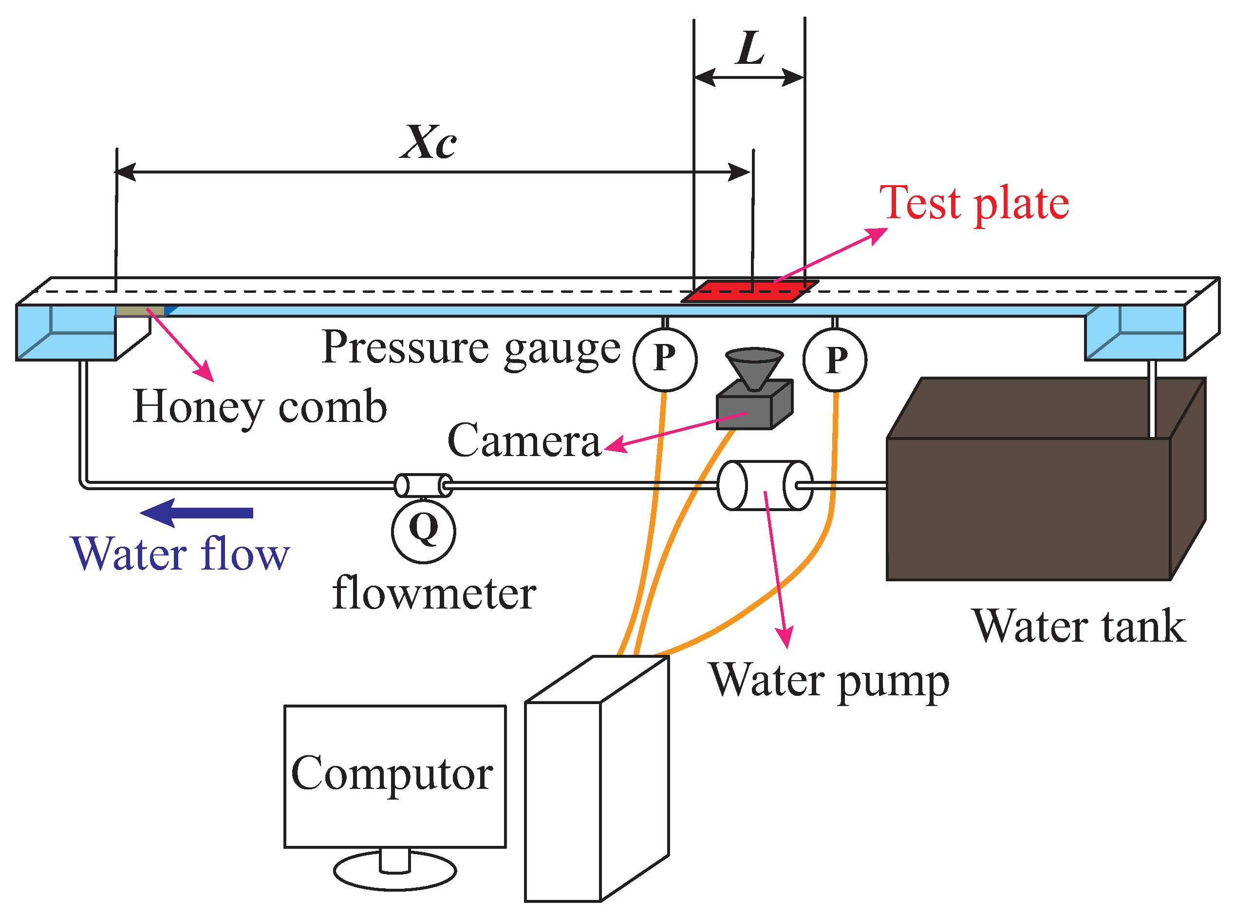
The schematic of the water tunnel where the experiments are conducted is presented in Figure 1. The water tunnel is comprised of two settling chambers, the upstream chamber and the downstream chamber. These two chambers are used to suppress the turbulence and pressure fluctuation in the tunnel. The length, width, and height of the chambers are 60 mm, 40 mm, and 40 mm, respectively. In order to break the vortexes flowing into the tunnel, a honeycomb is connected next to the upstream chamber. The tunnel between those two chambers is 1320 mm long and its cross-section is square. The width and height of the tunnel are 40 mm and 10 mm, respectively. The distance between the entrance of the tunnel and the center of the test plate is mm. This distance is reserved for the development of the turbulent boundary layer. The test plate is 240 mm long and 34 mm wide. The test plate is fixed on the upper wall of the tunnel and faces downward. The buoyancy experienced by the air points upward and prevents the air from leaving the grooves.
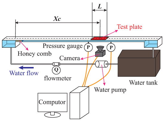
Figure 1.
Schematic of the water tunnel.
The drag reduction rate is characterized by the pressure drop between two pressure gauges and is calculated as below
where the and are the total frictional area between the two pressure gauges and the area of the test plate, respectively. and are the pressure drop of the test sample and the smooth sample, respectively. The total frictional area is comprised of an upper wall, a lower wall, and two side walls. The test plate is on the upper wall. Thus, .
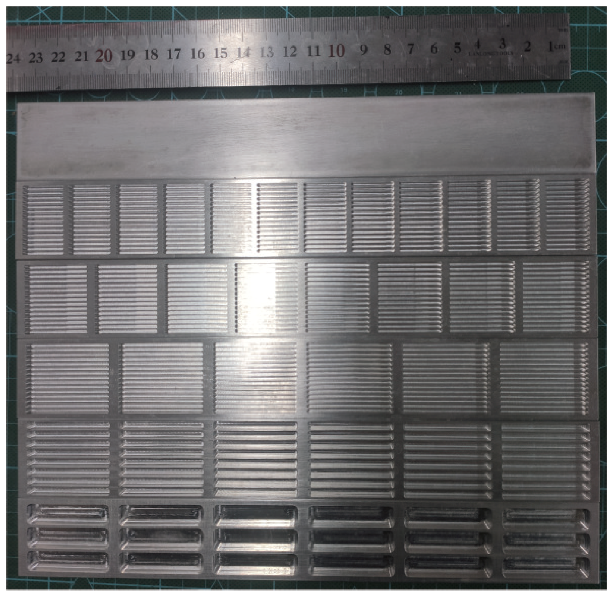
The range of the pressure gauges is 40 kPa and the minimum variation in pressure they can detect is 5 Pa. The two pressure gauges are connected to the computer and their data are synchronously collected. The sampling frequency and sampling time are 20 Hz and 40 s, respectively. For each sample, the pressure data are collected 5 times. Samples used in this work are presented in Figure 2. These samples are T6061 aluminum alloy and the grooves are obtained by milling. The smooth sample is polished before it is tested. The grooved samples are tested directly. The bulk velocity is calculated as , where the Q and S are the volume flow rate and the area of the tunnel cross-section, respectively. The volume flow rate Q is measured with a flow meter. The range and sensitivity of the flow meter are 5 m3/h and 0.001 m3/h, respectively. The water in the tunnel is accelerated by a DC water pump. The flow rate can be adjusted through the duty of the pulse-width modulation (PWM) and the maximum flow rate is 0.90 m3/h.
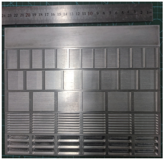
Figure 2.
Samples used in this work. The first one is a ruler. The 2nd one to the 7th one are the samples Smooth, #1, #2, #3, #4, and #5 that are listed in Table 1.
The parameters of the tested samples in this work are listed in Table 1. The length, width, and depth are the streamwise distance between the center of the adjacent grooves, the spanwise distance between the center of the adjacent grooves, and the depth of the grooves, respectively. The length and width of the grooves are 90 percent of the streamwise distance and spanwise distance, respectively. The Reynolds number, , is calculated as below
where the and are the height of the tunnel and the bulk velocity in the tunnel, respectively. The mm.

Table 1.
Parameters of the tested samples. Milimeters are used as the length unit here.
2.2. Numerical Details
The numerical simulation was performed with the Ansys Fluent 2021 R1. The computational domain of the numerical simulation is presented in Figure 3. It is impossible to perform computation on the domain which is the same as the samples used in the experimental measurement. The reason is that the samples used in the experimental measurement comprise dozens of grooves. If the computational domain of the experimental samples is used, the grid quantity might comprise hundreds of millions of elements. The huge number of grid elements requires an extremely excellent computer to accomplish the calculation. Thus, it is impossible to perform the calculation on the domain which is the same as the samples used in the experimental measurement. The computational domain used here is a single groove. The boundary conditions applied here are velocity inlet, pressure outlet, and periodic boundary for the front and back wall. The other walls are set as no-slip boundaries. The gravity is on the −y-axis. The velocity inlet was calculated from a channel with the same cross-section as Figure 3. The calculated channel length is set as (the distance between the entrance of the water tunnel and the center of the test plate presented in Figure 2). The height of the computational domain is the same as the height of the water tunnel (10 mm). The length and width of the computational domain are the same as the groove dimensions used in the water tunnel experiment.
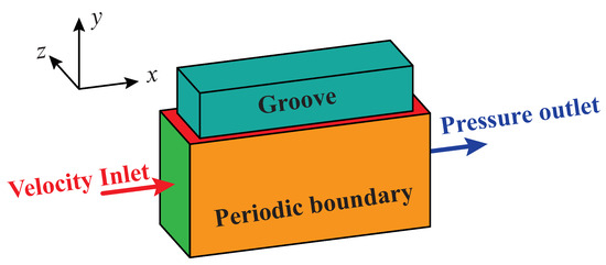
Figure 3.
The computational domain of the numerical simulation.
The calculation is based on the Navier–Stokes equations. The Navier–Stokes equations are written as below
where , p, are the density, static pressure, and viscosity of the fluid, respectively. is the velocity vector. and are the strain tensor and unit matrix, respectively. The transport equations for the standard k- model are written as follows
where k and are the turbulence kinetic energy and its rate of dissipation, respectively. and are added term due to the generation of the turbulence kinetic energy. represents the turbulent viscosity. and are the turbulent Prandtl numbers for k and , respectively. The VOF model is applied here to model the air–water multiphase flow. The tracking of the air–water interface is accomplished by the solution of the continuity equation for the volume fraction of the phases. For the phase, this equation has the following form
where the and represent the volume fraction and source term of the phase, respectively. The represents the mass transfer from the phase to the phase. The volume fraction is constrained by . In this work, = 0 represents water and = 1 represents air. The VOF model is coupled with the NS equation by adding a surface tension to the right hand of Equation (4). The surface tension is calculated as follows
The standard wall treatment is applied because the y* at the wall is larger than 11.25, which meets the requirement of the wall treatment approach. In order to reduce the calculation error, the residual of each flow field quantity is set to be . In order to guarantee the calculation convergence, the adaptive time step is applied. The time step varies from to . The time step is adjusted in order to satisfy . The SIMPLE pressure–velocity coupling scheme is chosen. The spatial discretization of the gradient, pressure, momentum, volume fraction, turbulent kinetic energy, and turbulent dissipation rate are Least Squares Cell-Based, PRESTO, Second-Order Upwind, Geo-Reconstruct, First-Order Upwind, and First-Order Upwind, respectively.
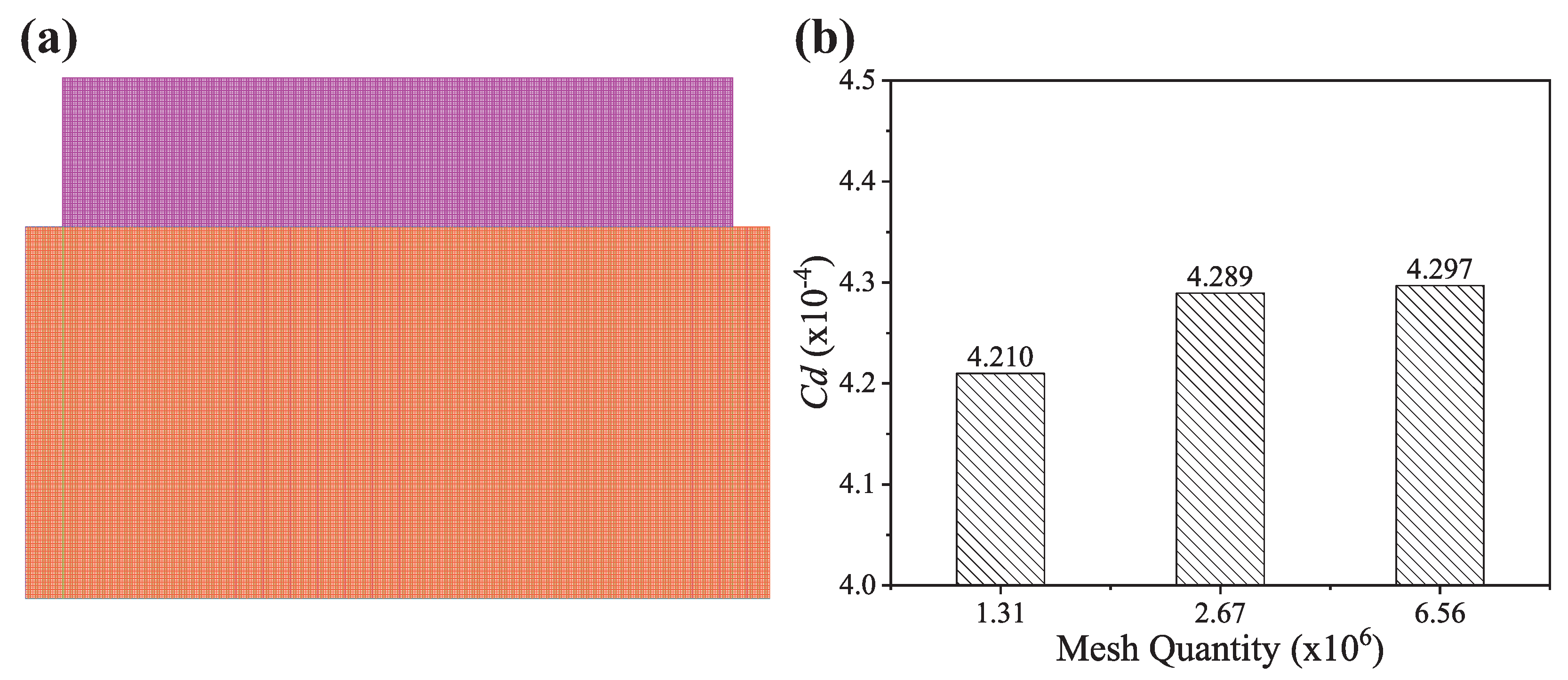
The structural mesh is applied here to improve the mesh quality (Figure 4a). All the meshes are cubes of the same size. The verification of the mesh independency is presented in Figure 4b. The smooth surface is used in the verification. The result shows that the mesh number of 2.76 × 10⁶ and 6.56 × 10⁶ exhibits the same drag coefficient, which indicates that the mesh density of 2.67 × 10⁶ meshes is adequate for the computation accuracy.
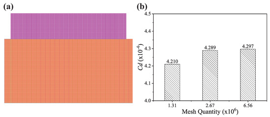
Figure 4.
The structural mesh (a) and mesh independency (b).
3. Results and Discussion
In this section, the following contents are discussed. Firstly, the trapped air stability is discussed. Then, the numerical simulation is applied to explain the drag reduction mechanism and optimize the groove length. Finally, experimental measurements are presented to confirm our design.
3.1. The Trapped Air Stability
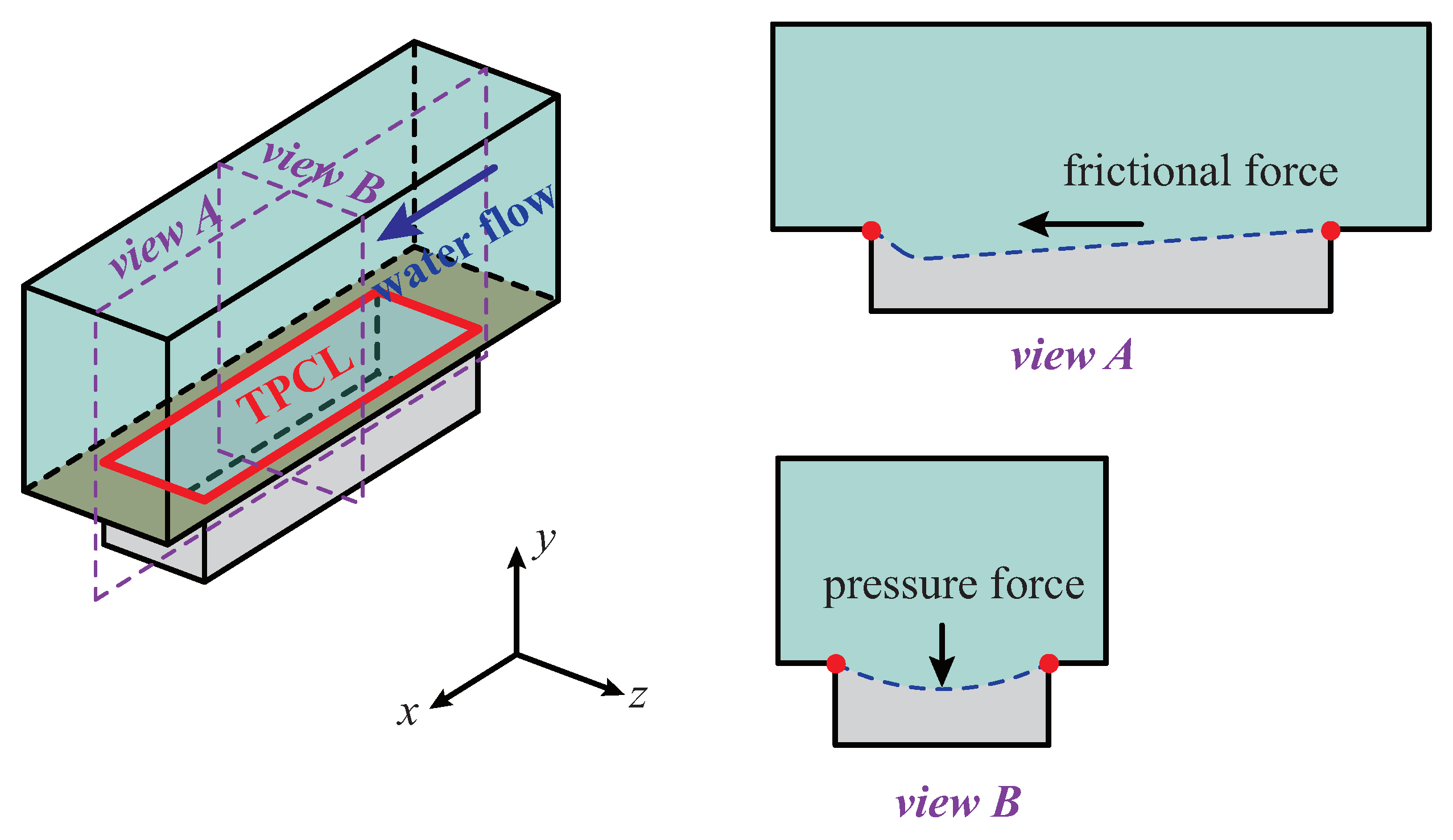
The discussion of the trapped air stability starts from the force balance. The force balance is depicted in Figure 5. The trapped air experiences the capillary force and the frictional force and the pressure force . The trapped air reaches a stable state when these three forces reach balance. The capillary force is produced by the surface tension and is supported by the three-phase contact line (TPCL). The capillary force is estimated as below
where the and the and the and the are the surface tension of the water and the unknown factors in the x direction and y direction and z direction, respectively. The and and are the unit vectors in the x direction and y direction and z direction, respectively. The unknown factors, the and the and the , are only decided by the shape of the air–water interface S and range from −2 to 2. On the right hand of Equation (11), the first term and the second term and the third term are the capillary force components in the x direction and y direction and z direction, respectively. For the flat or the symmetric air–water interface, these three factors will be 0. For the air–water interface shown in Figure 5view A, the will be negative, which means that the x component of the capillary force is in the direction. For the air–water interface shown in Figure 5view B, the will be positive, which means that the y component of capillary force is in the y direction.
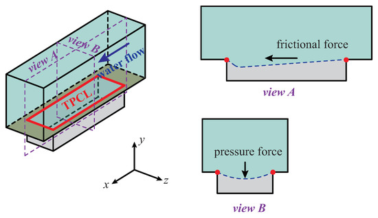
Figure 5.
Schematic of the force balance.
The capillary force is the only force that keeps the trapped air from being broken by the frictional force and the pressure force. The frictional force is produced by the shear stress between the flowing water and the trapped air and it can be evaluated as below
where the is the shear stress between the flowing water and the trapped air. The pressure force is produced by the pressure difference between the water and the air and it can be evaluated as below
where the () is the pressure difference between the water and the air. The trapped air reaches the stable state when . This produces two equations as below
In Equation (15), both the numerator and the denominator cancel by l and is ignored because for all the samples examined in this work.
The above analysis means that the groove length l and groove width w should be limited if the trapped air is going to stay stable. The limitations of the groove length l and the groove width w are written as below
The shear stress and the pressure difference are unknown variables. The known variable is the flow velocity . The unknown variables and can be related to the known variable . The shear stress of the air–water interface can be estimated to be proportional to the shear stress of the smooth surface. The shear stress can also be estimated as , where the is the characteristic length. The can be the boundary layer thickness (for wall-bounded plate flow) or the half of the channel height (for channel flow). Thus, Equation (16) can be rewritten as below
where the and are the proportionality coefficient. The pressure difference of the air–water interface is caused by the inertia force and can be estimated to be proportional with . Thus, Equation (17) can be rewritten as below
where the is the proportionality coefficient. The dimensionless groove length and groove width are defined as below
In this way, the unknown factors, and and and and , can be reduced to the factors and .
The represents the ratio of the frictional force to the capillary force. The trapped air would be destroyed and escape from the grooves if the exceeds the threshold . It can be found that the is the same as the Weber number , which represents the ratio of the inertia force () to the capillary force (). This indicates that the trapped air would be squeezed out of the grooves if the exceeds the threshold .
Now, it can be concluded that the groove dimensions should be limited if the trapped air is going to stay in a stable state. For a specific velocity , the groove length l and groove width w should be kept below a threshold. This is why the discrete grooves are employed here. By limiting the groove length and groove width, air instability and escape are possibly avoided.
3.2. The Numerical Result
3.2.1. The Drag Reduction Mechanism
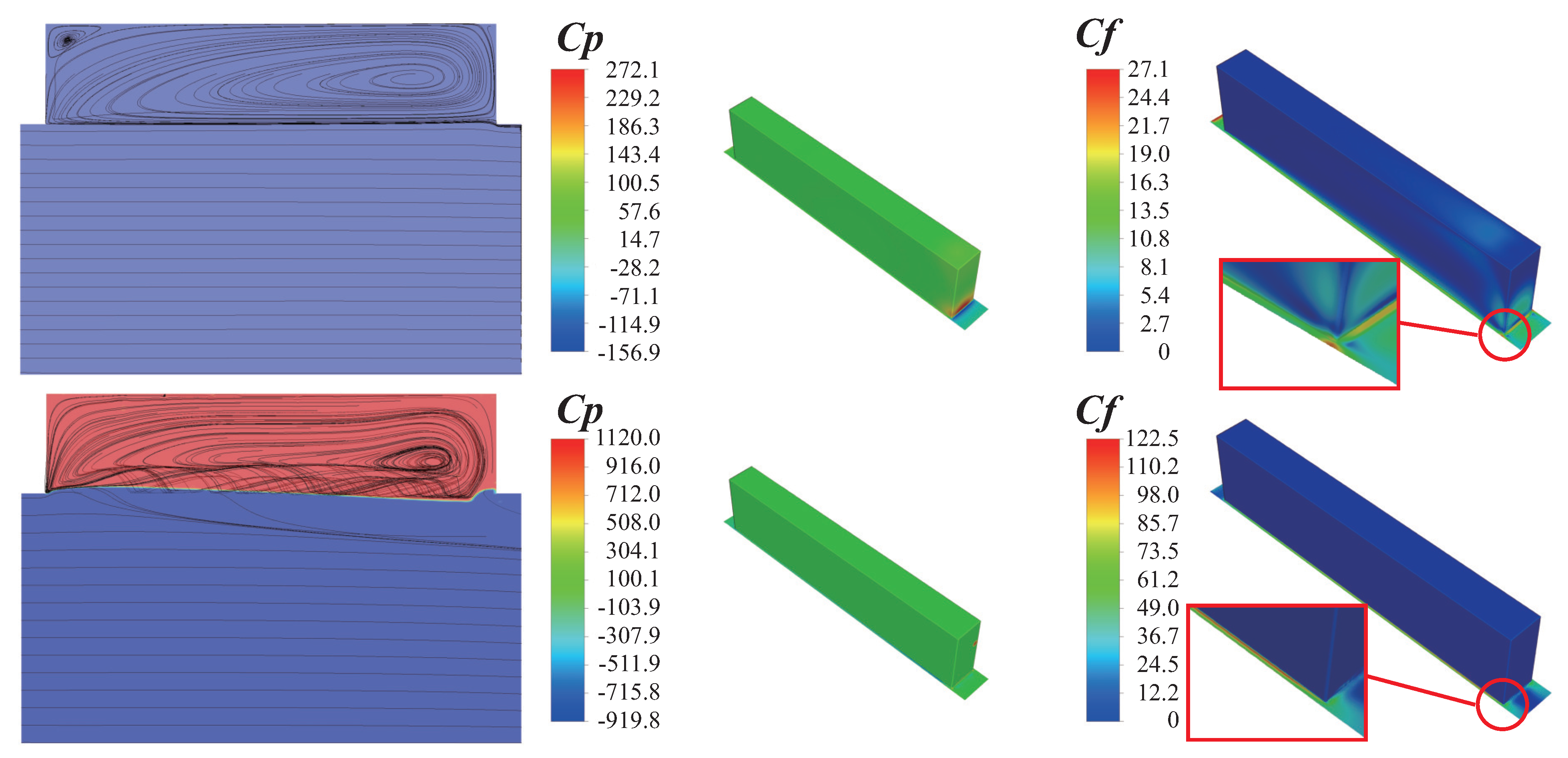
In order to explain the drag reduction mechanism, the groove of sample #1 (Table 1) is calculated. The smooth surface, groove filled with water, and groove filled with air are compared. In the first column of Figure 6, the pathline of the flow field is presented. Vortex grows in both the grooves filled with water and air. In the mid column and right column of Figure 6, the pressure coefficient and frictional coefficient are presented. The pressure coefficient or frictional coefficient is defined as
where the F is the pressure drag or frictional drag. The A is the projected area. It is clearly shown in the mid-column that there is a high-pressure region at the trailing edge of the groove filled with water. And the phase field in the left column also shows that the air–water interface is pressed into the groove. In the right column, the friction coefficient is presented. The friction coefficient is small in the groove filled with water or air. The friction coefficient at the top of the groove filled with water is higher than that of the groove filled with air. This is because the air filled in the groove. The existence of air causes slip velocity at the air–water interface. The nonzero slip velocity increases the velocity gradient at the top of the groove and thus causes a high friction coefficient.

Figure 6.
The pathline and phase field (left column), pressure coefficient (mid column), and friction coefficient (right column). The first row is the groove filled with water and the second row is the groove filled with air. In the left column, the water is represented by blue color, the air is represented by red color.
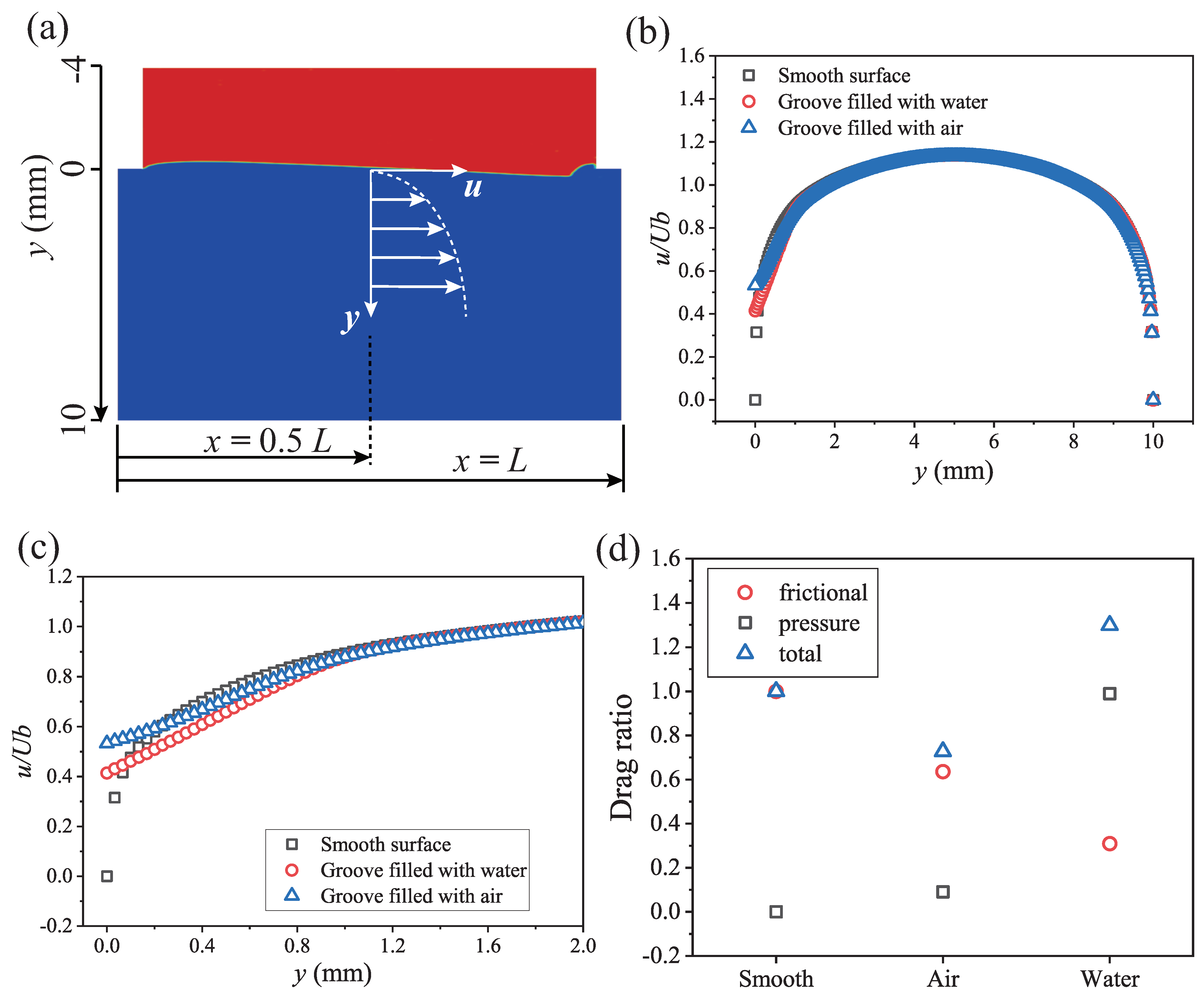
The velocity profile along the y-axis of the smooth surface, groove filled with water and groove filled with air is presented in Figure 7b,c. For the smooth surface, the velocity is 0 at . For the groove filled with water or air, the velocity is greater than 0 at y = 0, which means the slip velocity is caused by the vortex (Figure 6). The slip velocity leads to the intensified friction coefficient on the top of the groove (Figure 6). The velocity gradient of the smooth surface is the largest among these three samples, which means that the smooth surface experiences large frictional drag. The velocity gradient of the groove filled with air is the smallest among these three samples. The velocity gradient of the groove filled with water is smaller than the smooth surface and is larger than the groove filled with air. This indicates that the existence of a vortex in the groove can reduce the frictional drag.
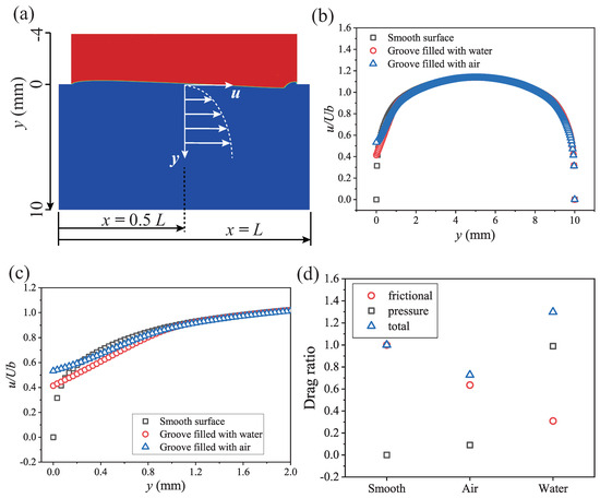
Figure 7.
The velocity profile along y-axis (b,c) and the ratio of the drag component (d). The y axis is chosen at x = 0.5 L and y = 0 is set at the top of the groove, as is shown in (a). (c) is the enlarged profile near y = 0.
In Figure 7d, the drag ratio of the drag component to the total drag of the smooth surface is presented. The smooth surface is smooth and the frictional drag ratio and pressure/drag ratio are 1 and 0, respectively. The friction drag ratio, pressure/drag ratio, and total drag ratio of the groove filled with air are 0.64, 0.09, and 0.73, respectively. The drag reduction of the groove filled with air is 27%. The friction drag ratio, pressure/drag ratio, and total drag ratio of the groove filled with water are 0.31, 0.99, and 1.30, respectively. The drag reduction of the groove filled with water is −30%. Though the velocity gradient of the groove filled with air is smaller than that of the groove filled with water, the slip velocity of the groove filled with air is larger than that of the groove filled with water. The large slip velocity leads to a large friction coefficient on the top of the groove (Figure 6). Thus, the friction drag ratio of the groove filled with air is larger than that of the groove filled with water. This means that the frictional drag reduction of the groove filled with water is better than that of the groove filled with air. But as is shown in Figure 6, there is a high-pressure region at the trailing edge of the groove filled with water. This means that the groove filled with water will introduce pressure drag. The pressure/drag ratio of the groove filled with water is larger than 1, which exceeds the reduced frictional drag and produces a drag increase. The pressure/drag ratio of the groove filled with air is larger than 0.09, which is smaller than the reduced frictional drag and produced the drag reduction. This means that the drag reduction is produced by the reducing frictional drag caused by the vortex in the groove. It also reveals the significant role of the trapped air in the groove. The trapped air in the groove will not only reduce the frictional drag but also mitigate the introduced pressure drag. And the groove wetted by water will cause the drag reduction failure.
3.2.2. Optimizing the Groove Length for Better Drag Reduction
In order to optimize the groove length for better drag reduction performance, the groove dimensions of the sample # 1 and # 2 and # 3 and # 4 (Table 1) are calculated and the result is presented in Figure 8 and Figure 9. In Figure 8, the phase field for the groove with different lengths is presented. For the grooves with lengths of 18 mm and 36 mm, the trapped air is pressed into the grooves at the trailing edge. For the grooves with lengths of 54 mm and 72 mm, the trapped air is stretched by the flowing water and air beads occur. The total simulated time is 0.25 s and it is hard to adjudge from the simulation whether the trapped air will escape or not. In Figure 9, the drag ratio and drag reduction rate are presented. The pressure/drag ratio of these grooves is smaller than 0.1 and the total drag is dominated by the frictional drag. The frictional drag reaches the maximum at the length of 54 mm and then starts to decrease. The drag reduction rates are 27.3%, 30.6%, 5.6%, and 8.5% for grooves with lengths of 18 mm, 36 mm, 54 mm, and 72 mm, respectively. The drag reduction rate reaches the maximum at the groove length of 36 mm.
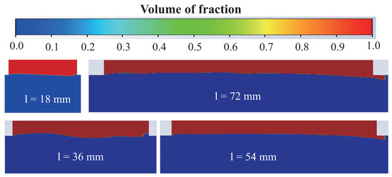
Figure 8.
The phase field, where 0 represents water and 1 represents air.
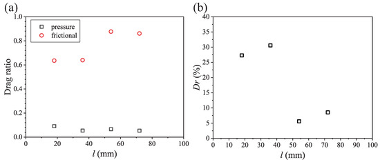
Figure 9.
The drag ratio (a) and drag reduction rate (b) varying with the groove length l.
3.3. The Experimental Result
3.3.1. The Repeatability of the Pressure Drop Measurements
In Figure 10, the five pressure drop measurements of the smooth sample and their average are presented. For each single measurement, the sampling time and sampling frequency are 40 s and 20 Hz. That means each single pressure drop measurement includes about 800 data points. For each single measurement, the pressure drop is the average of the 800 data points. The five pressure drop measurements are 144.0 Pa, 139.3 Pa, 134.8 Pa, 140.3 Pa, 141.0 Pa. The average and the standard error of these pressure drops are 139.9 Pa and 3 Pa, respectively. The error percentage is 2.1%, confirming the repeatability of the pressure drop measurements.
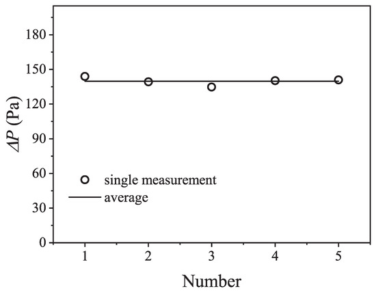
Figure 10.
The five single measurements and average of the pressure drop.
3.3.2. The Influence of the Groove Length on the Trapped Air Stability and Drag Reduction
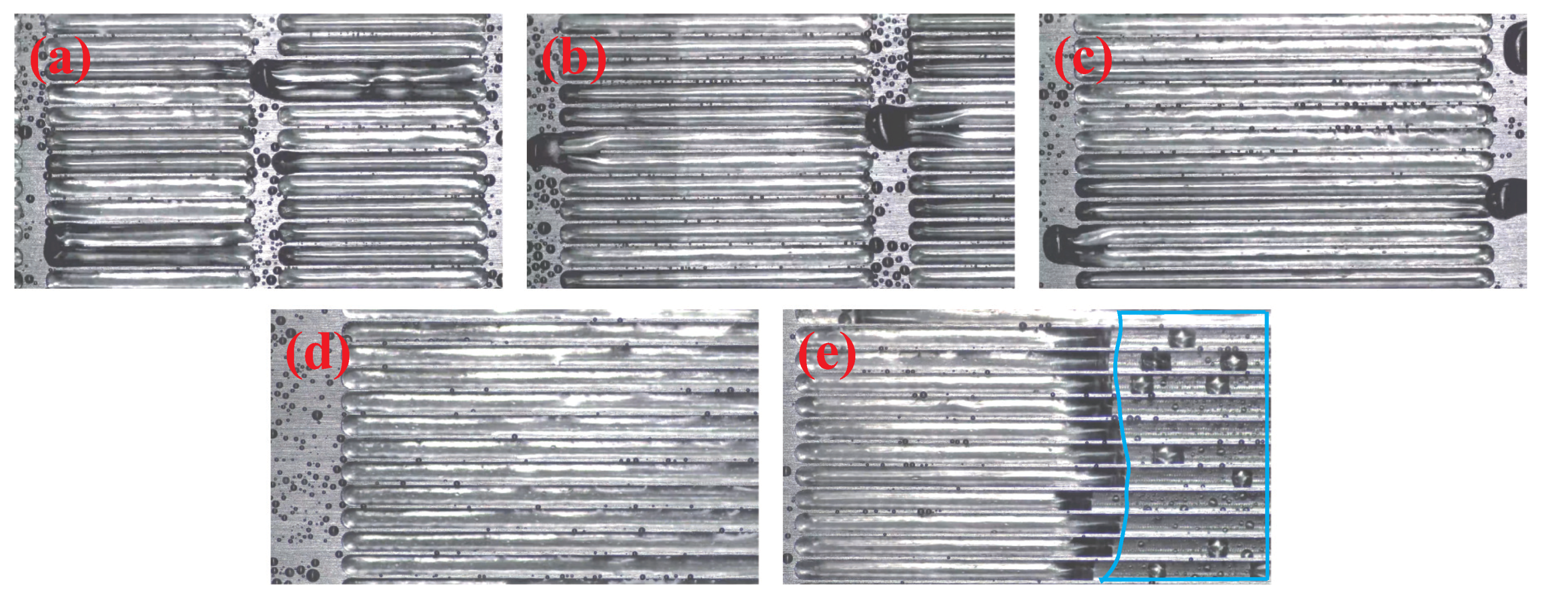
In Figure 11, the trapped air stability in the grooves with different lengths is presented. The trapped air is intact when the groove length l is less than 54 mm (Figure 11a–d). The grooves are wetted when the groove length l is greater than 72 mm (Figure 11e). The result indicates that the grooves with lengths less than 72 mm can successfully avoid the air escape at the Reynolds number = 2500. It can also be found that air beads hang at the trailing edge of the grooves for the groove lengths of 18 mm and 27 mm and 36 mm (Figure 11a–c). This indicates that the frictional force caused by the flowing water is limited and the capillary force provided by the TPCL is abundant and supports the hanging air beads. The air beads disappear when the groove length increases to 54 mm. This means that the frictional force caused by the flowing water reaches the maximum capillary force and the air beads can no longer hang at the trailing edge of the grooves. The experimental result confirms our analysis that the discrete grooves with limited length can successfully avoid air escape.

Figure 11.
The trapped air stability in the grooves. The groove length are 18 mm (a), 27 mm (b), 36 mm (c), 54 mm (d), and 72 mm (e). Grooves wetted by water are circled with blue lines.
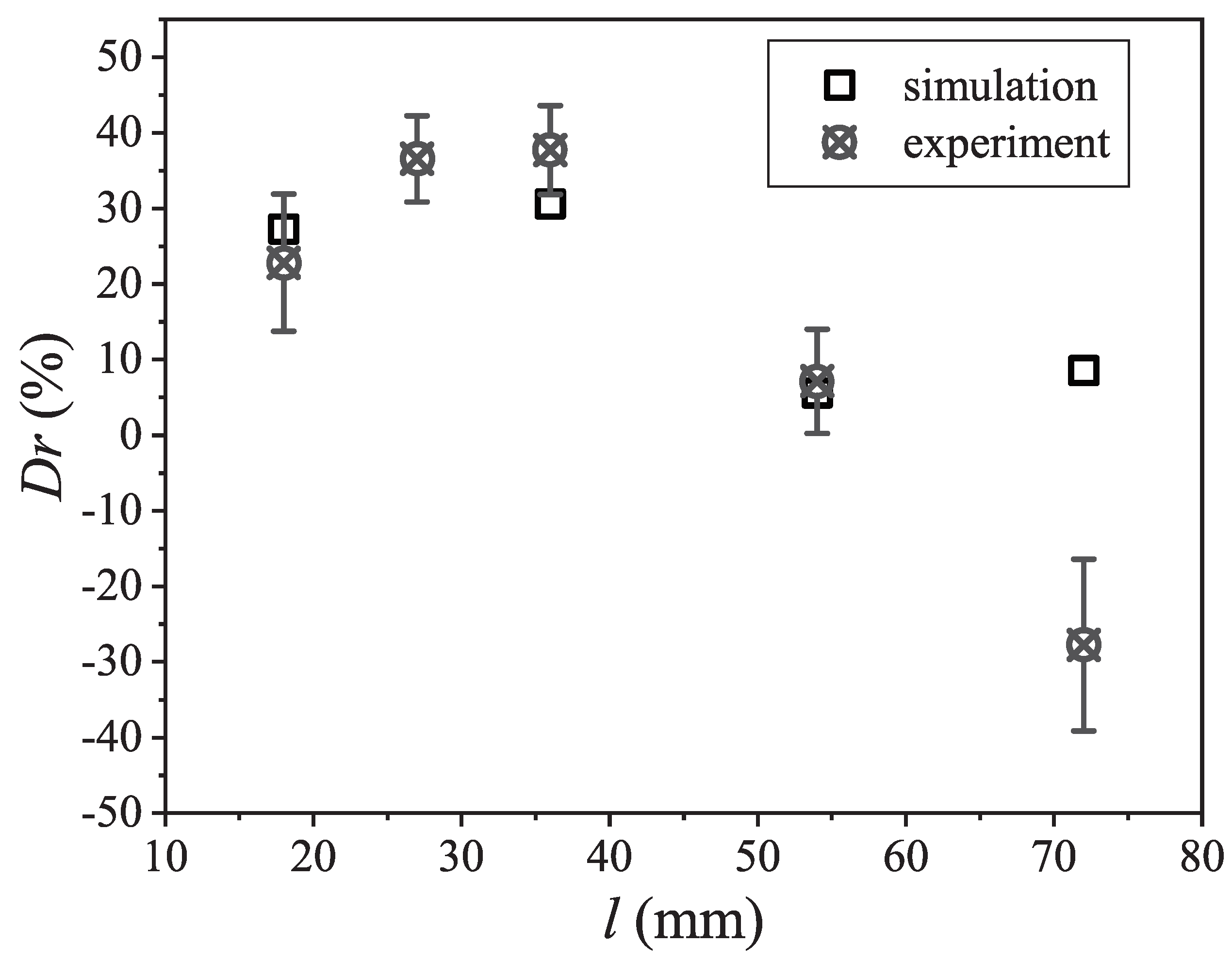
In Figure 12, the drag reduction rate varying with the groove length is presented. The is 22.8% for the groove length of 18 mm. The increases to 36.5% and 37.7% at the groove length of 27 mm and 36 mm, respectively. The starts to decrease when the groove length exceeds 36 mm. The is 7.1% for the groove length of 54 mm. The is −27.7% for the groove length of 72 mm, which means drag increase. The result shows that the discrete grooves exhibit drag reduction when the is 100% and exhibit drag increase when the is less than 100%. The maximum drag reduction rate of 37.7% is obtained at the groove length of 36 mm. This is consistent with the existing works that the drag reduction rate is related to the trapped air coverage rate [8,11,12]. The result of the simulation is also presented in Figure 12. The result shows that the simulation result is within the experimental error range except for the groove with a length of 72 mm. The exception is caused by the trapped air escape. In the experiment, the trapped air escapes from grooves, and the grooves are wetted (Figure 11). However, in the numerical simulation, the simulated time is short and the air escape is not found (Figure 8). Thus, the numerical result shows drag reduction while the experimental result shows drag increase. The result confirms the numerical simulation and the experimental measurements. For the less than 100%, the trapped air is squeezed out from the grooves by the water and the wetted grooves introduce extra pressure drag. Thus, the drag increase is produced at the less than 100%.

Figure 12.
The drag reduction rate varying with the groove length l.
In Figure 13a, the influence of the groove length on the trapped air coverage rate is presented. The trapped air coverage rate is calculated as below
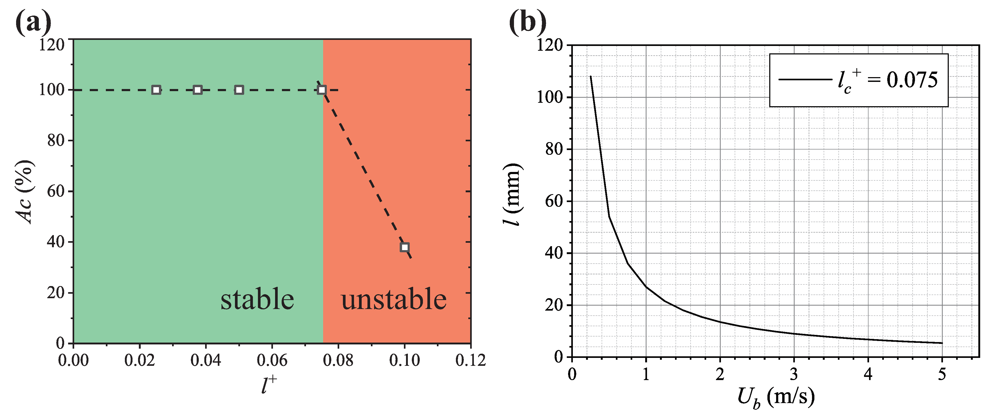
The is 100% for the intact trapped air. For the dimensionless groove length of 0.1 (72 mm), the is 37.9%. We regard the trapped air in the grooves with length ( 54 mm) as a stable state and the trapped air in the grooves with length ( 54 mm) as an unstable state. That means = 0.075. By employing the Equations (18) and (20), the threshold of the groove length at different velocity is obtained and is plotted in Figure 13b. For groove lengths shorter than this threshold, the trapped air is stable. For groove lengths longer than this threshold, the trapped air might be unstable and escape from the grooves. The threshold of the groove length is 54 mm, 27 mm, 13.5 mm, and 5.4 mm at the velocity of 0.5 m/s, 1.0 m/s, 2.0 m/s and 5.0 m/s, respectively.
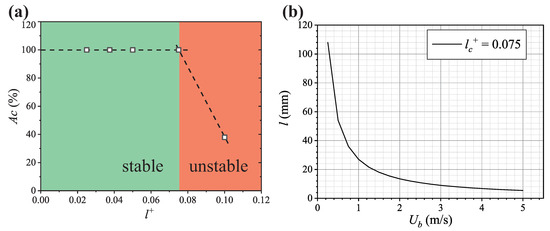
Figure 13.
The trapped air coverage rate varying with the dimensionless groove length (a) and the threshold of the groove length at different velocity (b).
3.3.3. The Influence of the Groove Width on the Trapped Air Stability and Drag Reduction
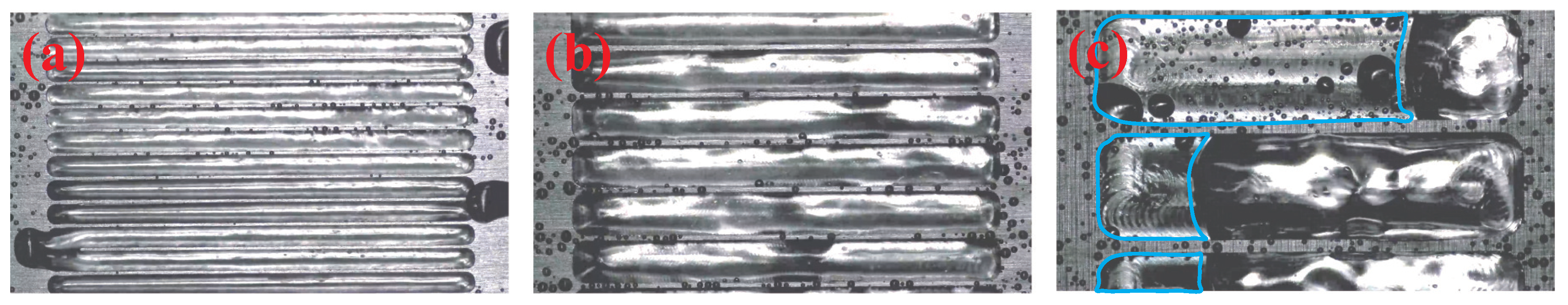
In Figure 14, the trapped air stability in the grooves with different width is presented. The result shows that the trapped air is intact for the grooves with width narrower than 3.6 mm (Figure 14a,b). The air instability occurs at the trailing edge of the grooves for the groove width of 9 mm. The result indicates that the air instability is avoided by limiting the groove width. And this is consistent with the discussion about the trapped air stability in Section 3.1. The air instability is caused by the pressure difference. It is shown in Section 3.2.1 that there is a high pressure region at the trailing edge of the grooves. This high pressure region pressed the air–water interface into the grooves and caused instability.

Figure 14.
The trapped air stability in the grooves. The groove width are 1.8 mm (a), 3.6 mm (b), and 9 mm (c). Grooves wetted by water are circled with a blue line.
In Figure 15, the drag reduction rate varying with the groove width is presented. The of the grooves with width of 1.8 mm is 37.7%. The of the grooves with width of 3.6 mm is 38.2%. The of the grooves with width of 9 mm is −86.0%. According to the trapped air morphology in Figure 14c, the wetted grooves are related with the drag increase. It is shown in Figure 5 and Equation (13) that the pressure difference between the water and the trapped air is the cause of the wetted grooves. The flowing water reattaches to the solid wall at the trailing edge of the grooves and the accumulation of the momentum causes a high pressure region, as is shown in Figure 6. Thus, the air–water interface is pressed into the grooves and pressure drag is introduced. For the grooves with width of 1.8 mm and 3.6 mm, the trapped air is intact and no pressure drag is introduced into the grooves. Thus, both of them exhibit drag reduction. The best drag reduction rate is 38.2%, which confirms the drag reduction efficiency.
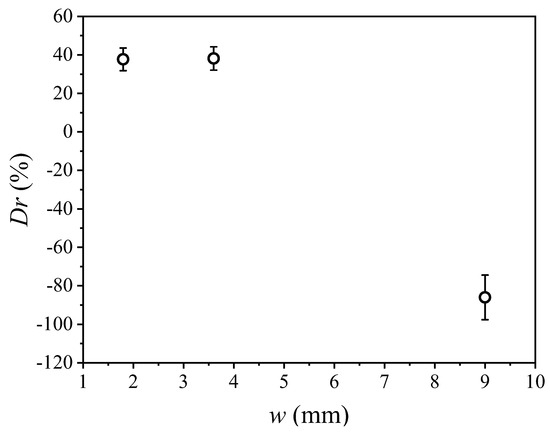
Figure 15.
The drag reduction rate varying with the groove width w.
In Figure 16a, the influence of the groove width on the trapped air coverage rate is presented. For the dimensionless groove width of 6.25 (1.8 mm) and 12.5 (3.6 mm), the trapped air in the grooves is intact and the trapped air coverage rate is 100%. For the dimensionless groove width of 31.25 (9 mm), the trapped air is unstable and the coverage rate is 59.3%. As is shown in Figure 15, the grooves with width of 12.5 (3.6 mm) exhibits the drag reduction rate of 38.2% and the trapped air in them are intact. Thus, we regard the trapped air in the grooves with width less than 12.5 (3.6 mm) as stable state and the trapped air in the grooves with width greater than 31.25 (9 mm) as unstable state. That means = 12.5. By employing Equations (19) and (21), the threshold of the groove width at different velocity is obtained and is plotted in Figure 14b. For groove width narrower than this threshold, the trapped air are stable. For groove width wider than this threshold, the trapped air might be unstable and be pressed into the grooves. The thresholds of the groove width are 3.6 mm, 0.9 mm, 0.23 mm, and 0.036 mm at the velocity of 0.5 m/s, 1.0 m/s, 2.0 m/s, and 5.0 m/s, respectively.
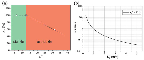
Figure 16.
The trapped air coverage rate varying with the dimensionless groove width (a) and the threshold of the groove width at different velocity (b).
3.3.4. The Influence of the Groove Depth on the Trapped Air Stability and Drag Reduction
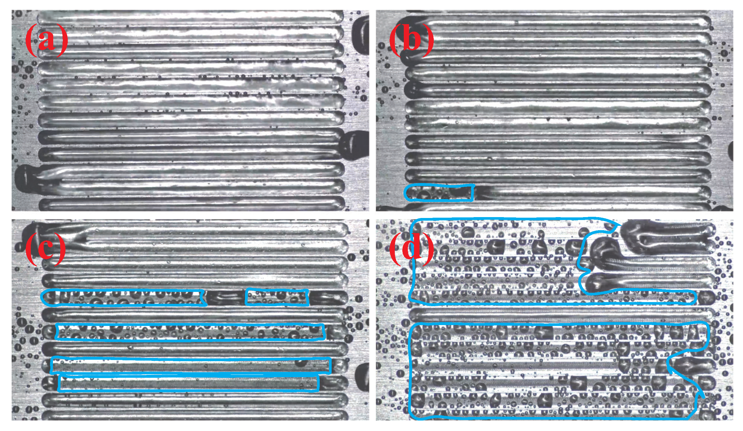
In Figure 17, the trapped air stability in the grooves with different groove depths is presented. The trapped air is intact for the groove depth of 4 mm. The grooves are gradually wetted when the groove depth decreases. As can be found in Figure 17b–d, the wetted area gets larger and larger. The wetted area occurs at the trailing edge of the grooves. This result is similar to the result of Figure 14c and we conclude that the wetted area is caused by the pressure force instead of the air dissolution. The pressure force presses the air–water interface and the chance of the air–water interface touching the bottom wall of the grooves increases when the groove depth decreases.
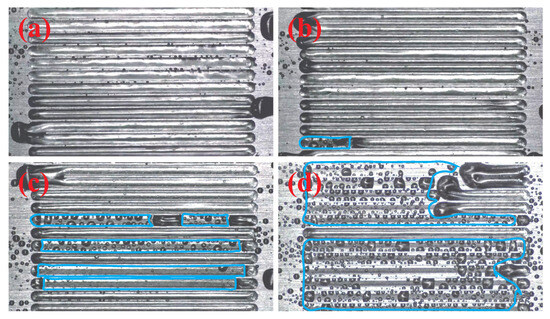
Figure 17.
The trapped air stability in the grooves. The groove depth are 4 mm (a), 2 mm (b), 1 mm (c), and 0.5 mm (d). Grooves wetted by water are circled with a blue line.
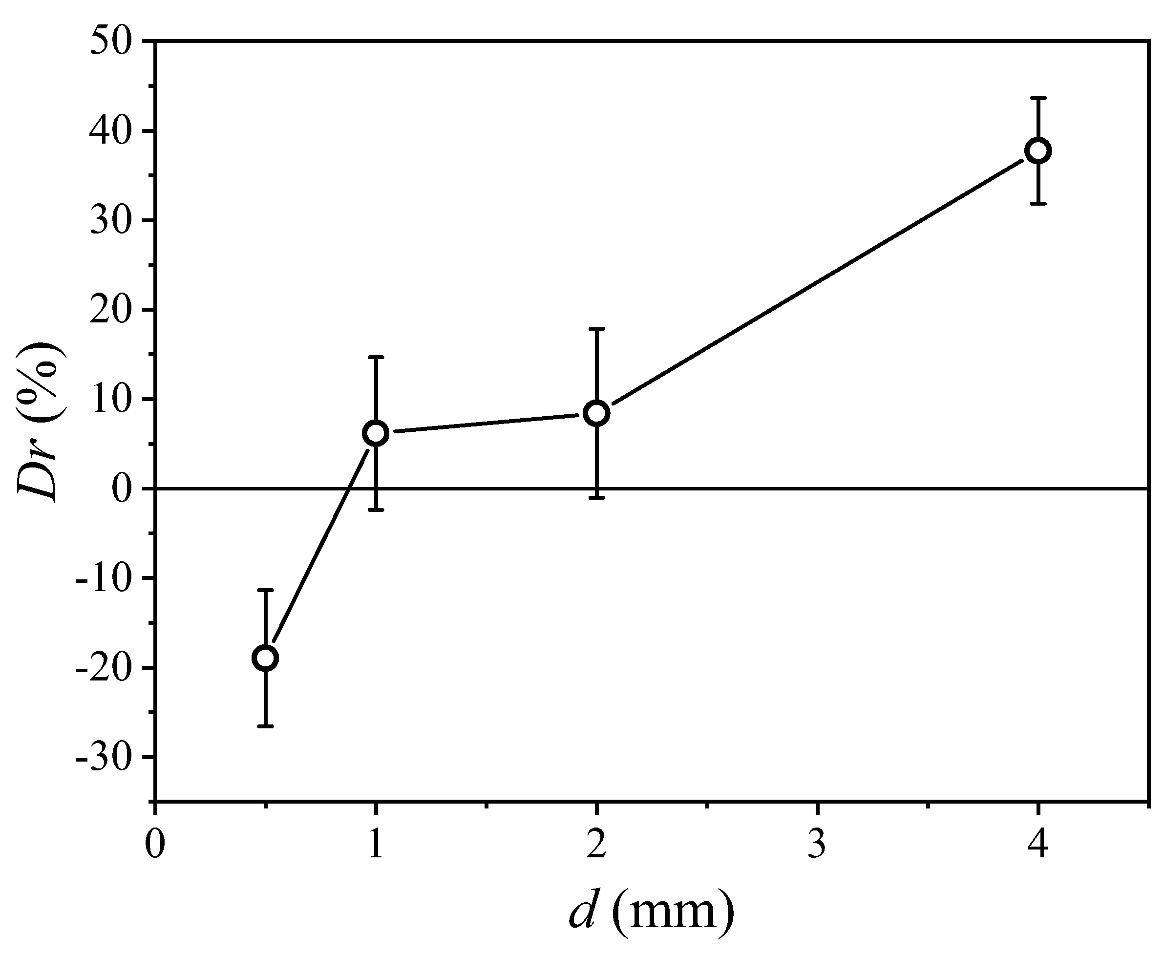
In Figure 18, the drag reduction rate varying with the groove depth is presented. The is 37.8% when the groove depth is 4 mm. The is 8.4% when the groove depth is 2 mm. The is 6.1% when the groove depth is 1 mm. The is −19.0% when the groove depth is 0.5 mm. As is illustrated in Section 3.3.3, the wetted grooves introduce pressure drag and cause drag increase. Thus, the drag reduction rate decreases when the wetted grooves increase.

Figure 18.
The drag reduction rate varying with the groove depth.
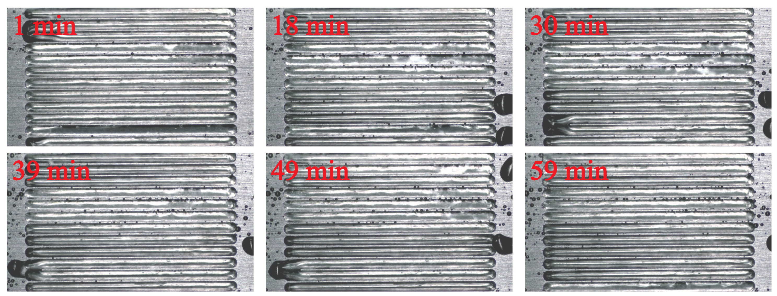
In order to verify that the deepened grooves can mitigate the air dissolution, the grooves with a depth of 4 mm are chosen and tested under the flowing water for 60 min. The result is presented in Figure 19. The result shows that the trapped air is intact and no obvious dissolution is found in the optical pictures. This result confirms that the air dissolution is negligible for the grooves with a depth of 4 mm and is successfully mitigated.
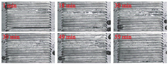
Figure 19.
The trapped air varying with time.
4. Conclusions
In this work, the discrete grooves are employed to trap air and reduce drag. The stability of the trapped air in the grooves is analyzed. The analysis is based on the force balance of the capillary force, frictional force, and pressure force. The analysis indicates that the trapped air escape is related to the groove length. Longer grooves produce larger frictional force, which causes the trapped air to escape. The trapped air instability is related to the groove width. Wider grooves produce a larger pressure force, which causes the trapped air instability. The analysis indicates that the way to avoid trapped air escape and instability is to limit the groove length and width.
The numerical simulation is applied to explain the drag reduction mechanism. The numerical simulation indicates that the vortex grows in the grooves. The formation of the vortex reduces the velocity gradient near the air–water interface and thus reduces the frictional drag. The grooves also introduce pressure drag. The introduced pressure drag is small if the grooves are filled with air. The introduced pressure drag exceeds the reduced frictional drag when the grooves are filled with water. The result shows that the grooves filled with air reduce the total drag while the grooves filled with water increase the total drag. The results emphasize that the grooves should be filled with air when they are applied to reduce drag.
The experimental measurements are conducted in a water tunnel to verify our design. The result shows that the trapped air escape is successfully avoided for the groove length less than 54 mm and the drag reduction of 37.7% is obtained. The maximum groove length at the wider velocity range is provided according to the analysis of the force balance. The trapped air instability is successfully avoided for the groove width less than 3.6 mm and the drag reduction of 38.2% is obtained. The maximum groove width at the wider velocity range is also provided. The result also shows that the deep grooves can successfully mitigate the trapped air dissolution. The deep grooves are examined for 60 min and the result shows that no obvious trapped air dissolution is found. The experimental result is consistent with the analysis and the numerical simulation. This work is meaningful for the underwater drag reduction application.
Author Contributions
Conceptualization, J.W.; methodology, D.W.; formal analysis, Y.N.; investigation, Y.N.; writing—original draft preparation, Y.N.; writing—review and editing, D.W. All authors have read and agreed to the published version of the manuscript.
Funding
This research was funded by the National Natural Science Foundation of China (NSFC) (Grant No. 52275200).
Institutional Review Board Statement
Not applicable.
Informed Consent Statement
Not applicable.
Data Availability Statement
The data that support the findings of this study are available from the corresponding author upon reasonable request.
Conflicts of Interest
The authors declare that there is no conflict of interest in publishing this work.
Abbreviations
The following abbreviations are used in this manuscript:
| Drag reduction rate | |
| trapped air coverage rate | |
| Bulk velocity | |
| TPCL | Three phase contact line |
References
- Zhang, X.; Zhang, D.Y.; Pan, J.F.; Li, X.; Chen, H.W. Controllable Adjustment of Bio-Replicated Shark Skin Drag Reduction Riblets. Appl. Mech. Mater. 2013, 461, 677–680. [Google Scholar] [CrossRef]
- Walsh, M.J.; Weinstein, L.M. Drag and Heat-Transfer Characteristics of Small Longitudinally Ribbed Surfaces. AIAA J. 1979, 17, 770–771. [Google Scholar] [CrossRef]
- Choi, K.S.; Clayton, B.R. The mechanism of turbulent drag reduction with wall oscillation. Int. J. Heat Fluid Flow 2001, 22, 1–9. [Google Scholar] [CrossRef]
- Gatti, D.; Guttler, A.; Frohnapfel, B.; Tropea, C. Experimental assessment of spanwise-oscillating dielectric electroactive surfaces for turbulent drag reduction in an air channel flow. Exp. Fluids 2015, 56, 110. [Google Scholar] [CrossRef]
- Rajappan, A.; McKinley, G.H. Cooperative drag reduction in turbulent flows using polymer additives and superhydrophobic walls. Phys. Rev. Fluids 2020, 5, 114601. [Google Scholar] [CrossRef]
- Fichman, M.; Hetsroni, G. Electrokinetic aspects of turbulent drag reduction in surfactant solutions. Phys. Fluids 2004, 16, 4346–4352. [Google Scholar] [CrossRef]
- Bidkar, R.A.; Leblanc, L.; Kulkarni, A.J.; Bahadur, V.; Ceccio, S.L.; Perlin, M. Skin-friction drag reduction in the turbulent regime using random-textured hydrophobic surfaces. Phys. Fluids 2014, 26, 18. [Google Scholar] [CrossRef]
- Xu, M.; Yu, N.; Kim, J.; Kim, C.J.C. Superhydrophobic drag reduction in high-speed towing tank. J. Fluid Mech. 2020, 908, A6. [Google Scholar] [CrossRef]
- Kim, H.N.; Kim, S.J.; Choi, W.; Sung, H.J.; Lee, S.J. Depletion of lubricant impregnated in a cavity of lubricant-infused surface. Phys. Fluids 2021, 33, 022005. [Google Scholar] [CrossRef]
- Yao, W.H.; Wu, L.; Sun, L.D.; Jiang, B.; Pan, F.S. Recent developments in slippery liquid-infused porous surface. Prog. Org. Coatings 2022, 166, 106806. [Google Scholar] [CrossRef]
- Park, H.; Sun, G.; Kim, C.J.C. Superhydrophobic turbulent drag reduction as a function of surface grating parameters. J. Fluid Mech. 2014, 747, 722–734. [Google Scholar] [CrossRef]
- Reholon, D.; Ghaemi, S. Plastron morphology and drag of a superhydrophobic surface in turbulent regime. Phys. Rev. Fluids 2018, 3, 104003. [Google Scholar] [CrossRef]
- Lay, K.A.; Yakushiji, R.; Mäkiharju, S.; Perlin, M.; Ceccio, S.L. Partial Cavity Drag Reduction at High Reynolds Numbers. J. Ship Res. 2010, 54, 109–119. [Google Scholar] [CrossRef]
- Mäkiharju, S.A.; Elbing, B.R.; Wiggins, A.; Schinasi, S.; Vanden-Broeck, J.M.; Perlin, M.; Dowling, D.R.; Ceccio, S.L. On the scaling of air entrainment from a ventilated partial cavity. J. Fluid Mech. 2013, 732, 47–76. [Google Scholar] [CrossRef]
- Hao, W.U.; Ou, Y.; Qing, Y.E. Experimental study of air layer drag reduction on a flat plate and bottom hull of a ship with cavity. Ocean Eng. 2019, 183, 236–248. [Google Scholar] [CrossRef]
- Qin, S.J.; Sun, S.; Fang, H.Z.; Wang, L.Y.; Chen, Y.; Wu, D.Z. Experimental and numerical investigation on the cavity regime and drag reduction of ventilated partial cavity. Ocean Eng. 2021, 234, 109257. [Google Scholar] [CrossRef]
- Liu, T.; Huang, B.; Wang, G.; Zhang, M.; Gao, D. Experimental investigation of the flow pattern for ventilated partial cavitating flows with effect of Froude number and gas entrainment. Ocean Eng. 2017, 129, 343–351. [Google Scholar] [CrossRef]
- Qu, Z.Y.; Yang, N.N.; Ma, G.H.; Yao, X.L.; Zhang, W.K.; Zhang, H.T.; Cheng, S.H.; Quan, X.B.; Chen, Y.Y. Experimental study on ventilated cavity flow at the tail of underwater vehicle under low surface tension. Ocean Eng. 2023, 267, 113230. [Google Scholar] [CrossRef]
- Aljallis, E.; Sarshar, M.A.; Datla, R.; Sikka, V.; Jones, A.; Choi, C.H. Experimental study of skin friction drag reduction on superhydrophobic flat plates in high Reynolds number boundary layer flow. Phys. Fluids 2013, 25, 14. [Google Scholar] [CrossRef]
- Kim, T.J.; Hidrovo, C. Pressure and partial wetting effects on superhydrophobic friction reduction in microchannel flow. Phys. Fluids 2012, 24, 112003. [Google Scholar] [CrossRef]
- Lv, P.Y.; Xue, Y.H.; Shi, Y.P.; Lin, H.; Duan, H.L. Metastable States and Wetting Transition of Submerged Superhydrophobic Structures. Phys. Rev. Lett. 2014, 112, 196101. [Google Scholar] [CrossRef] [PubMed]
- Ling, H.; Katz, J.; Fu, M.; Hultmark, M. Effect of Reynolds number and saturation level on gas diffusion in and out of a superhydrophobic surface. Phys. Rev. Fluids 2017, 2, 124005. [Google Scholar] [CrossRef]
- Hokmabad, B.V.; Ghaemi, S. Effect of Flow and Particle-Plastron Collision on the Longevity of Superhydrophobicity. Sci. Rep. 2017, 7, 41448. [Google Scholar] [CrossRef] [PubMed]
- Vullers, F.; Peppou-Chapman, S.; Kavalenka, M.N.; Holscher, H.; Neto, C. Effect of repeated immersions and contamination on plastron stability in superhydrophobic surfaces. Phys. Fluids 2019, 31, 012102. [Google Scholar] [CrossRef]
- Kim, H.; Park, H. Diffusion characteristics of air pockets on hydrophobic surfaces in channel flow: Three-dimensional measurement of air-water interface. Phys. Rev. Fluids 2019, 4, 074001. [Google Scholar] [CrossRef]


Disclaimer/Publisher’s Note: The statements, opinions and data contained in all publications are solely those of the individual author(s) and contributor(s) and not of MDPI and/or the editor(s). MDPI and/or the editor(s) disclaim responsibility for any injury to people or property resulting from any ideas, methods, instructions or products referred to in the content. |
© 2024 by the authors. Licensee MDPI, Basel, Switzerland. This article is an open access article distributed under the terms and conditions of the Creative Commons Attribution (CC BY) license (https://creativecommons.org/licenses/by/4.0/).