
Coupled Hydrodynamic and Biogeochemical Modeling in the Galician Rías Baixas (NW Iberian Peninsula) Using Delft3D: Model Validation and Performance

 , ,
, ,  , ,
, ,  ,
,  and
and 
Abstract
:1. Introduction
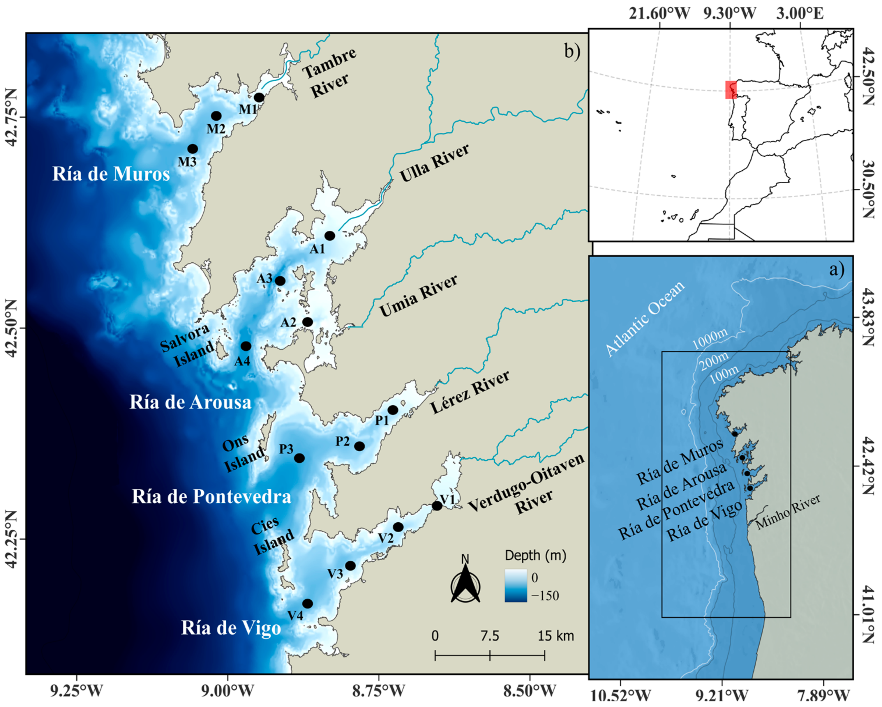
2. Study Area
3. Methodology
3.1. In Situ Data for Model Calibration and Validation
3.2. Numerical Modeling
3.2.1. Hydrodynamic Module
3.2.2. Water Quality Module
3.3. Model Calibration
4. Results
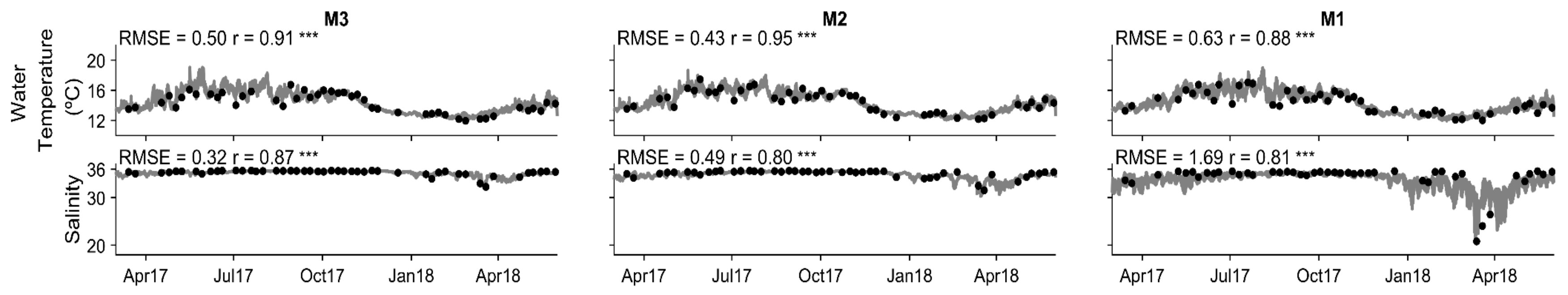
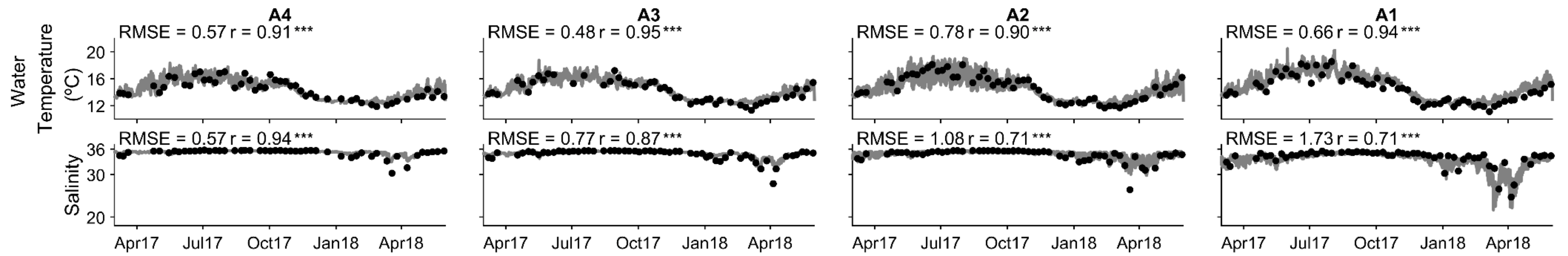
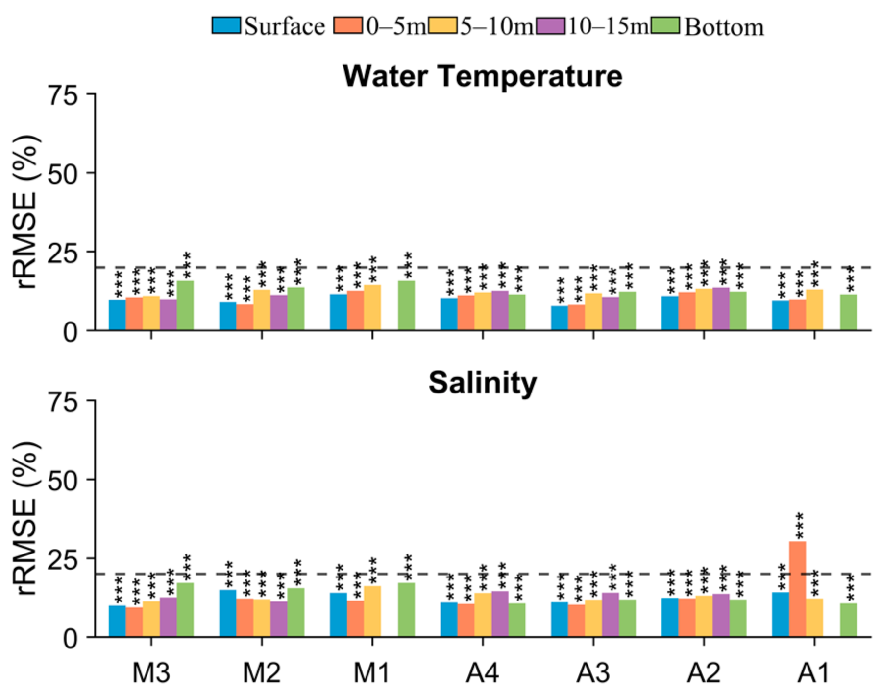
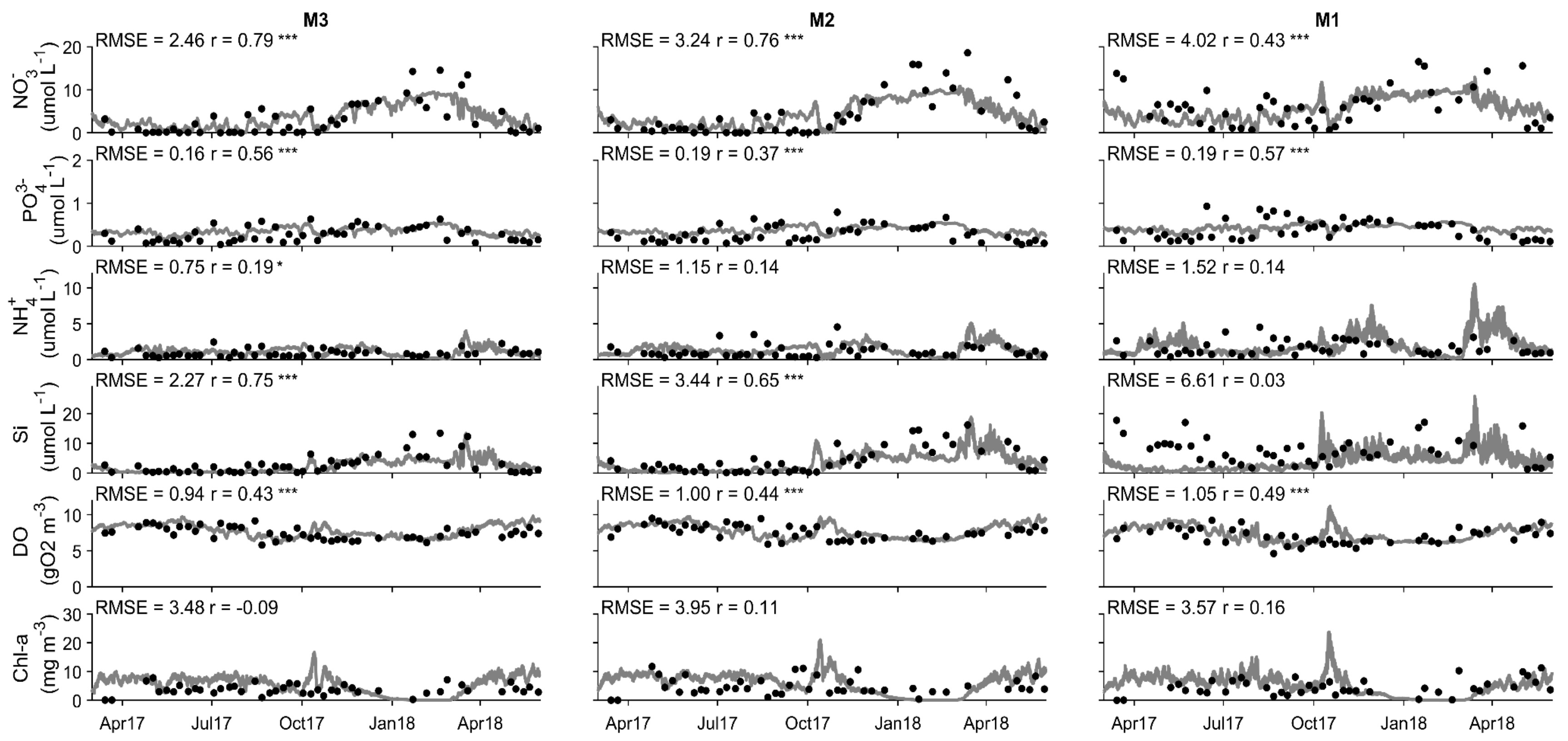
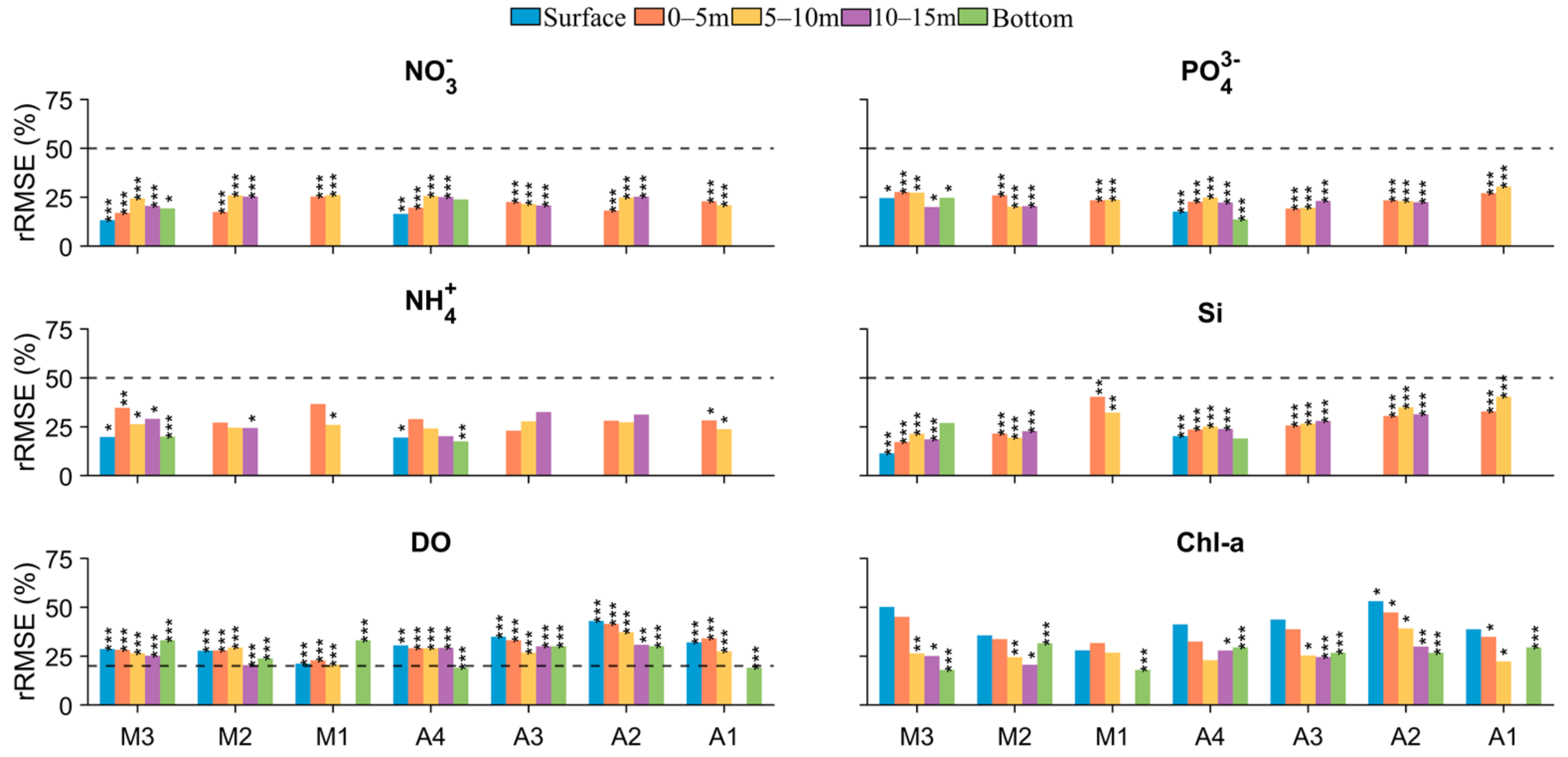
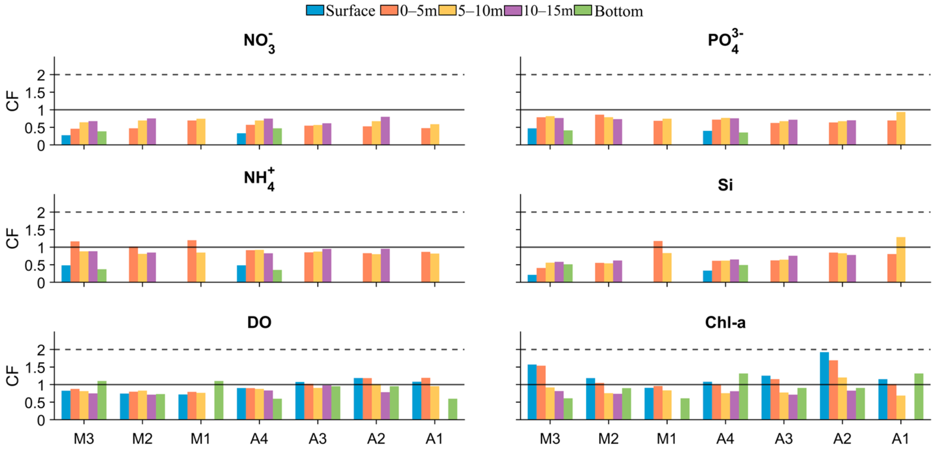
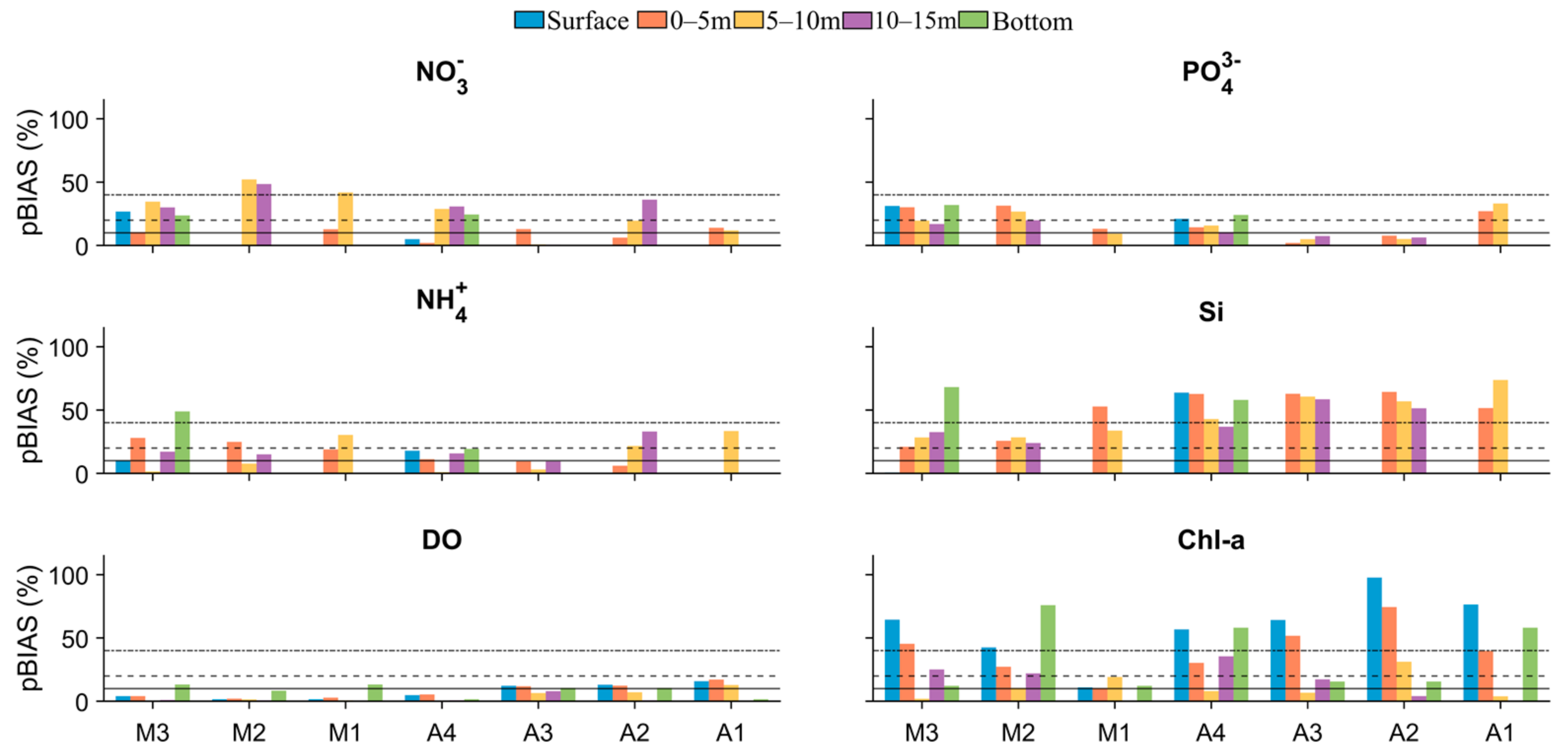
4.1. Model Calibration and Performance
4.2. Water Quality
5. Discussion
6. Conclusions
Supplementary Materials
Author Contributions
Funding
Institutional Review Board Statement
Informed Consent Statement
Data Availability Statement
Acknowledgments
Conflicts of Interest
References
- Kennish, M.J. Environmental threats and environmental future of estuaries. Environ. Conserv. 2002, 29, 78–107. [Google Scholar] [CrossRef]
- Wołowicz, M.; Sokołowski, A.; Lasota, R. Estuaries—A biological point of view. Oceanol. Hydrobiol. Stud. 2007, 36, 113–130. [Google Scholar] [CrossRef]
- Jackson, J.B. What was natural in the coastal oceans? Proc. Natl. Acad. Sci. USA 2001, 98, 5411–5418. [Google Scholar] [CrossRef]
- Cloern, J.E.; Abreu, P.C.; Carstensen, J.; Chauvaud, L.; Elmgren, R.; Grall, J.; Greening, H.; Johansson, J.O.R.; Kahru, M.; Sherwood, E.T.; et al. Human activities and climate variability drive fast-paced change across the world’s estuarine–coastal ecosystems. Glob. Chang. Biol. 2016, 22, 513–529. [Google Scholar] [CrossRef] [PubMed]
- Solomon, S.; Qin, D.; Manning, M.; Alley, R.B.; Berntsen, T.; Bindoff, N.L.; Chen, Z.; Chidthaisong, A.; Gregory, J.M.; Hegerl, G.C.; et al. Technical summary. In Climate Change 2007: The Physical Science Basis. Contribution of Working Group I to the Fourth Assessment Report of the Intergovernmental Panel on Climate Change; Cambridge University Press: Cambridge, UK; New York, NY, USA, 2007. [Google Scholar]
- Jennerjahn, T.C.; Mitchell, S.B. Pressures, stresses, shocks and trends in estuarine ecosystems–An introduction and synthesis. Estuar. Coast. Shelf Sci. 2013, 130, 9–20. [Google Scholar] [CrossRef]
- Hoegh-Guldberg, O.; Poloczanska, E.S. The effect of climate change across ocean regions. Front. Mar. Sci. 2017, 4, 361. [Google Scholar] [CrossRef]
- Canadell, J.G.; Jackson, R.B. (Eds.) Ecosystem Collapse and Climate Change; Springer: Cham, Switzerland, 2021. [Google Scholar] [CrossRef]
- Des, M.; Fernández-Nóvoa, D.; DeCastro, M.; Gómez-Gesteira, J.L.; Sousa, M.C.; Gómez-Gesteira, M. Modeling salinity drop in estuarine areas under extreme precipitation events within a context of climate change: Effect on bivalve mortality in Galician Rías Baixas. Sci. Total Environ. 2021, 790, 148147. [Google Scholar] [CrossRef] [PubMed]
- Castro-Olivares, A.; Des, M.; Olabarria, C.; DeCastro, M.; Vázquez, E.; Sousa, M.C.; Gómez-Gesteira, M. Does global warming threaten small-scale bivalve fisheries in NW Spain? Mar. Environ. Res. 2022, 180, 105707. [Google Scholar] [CrossRef]
- Álvarez-Salgado, X.A.; Gago, J.; Míguez, B.M.; Gilcoto, M.; Pérez, F.F. Surface waters of the NW Iberian margin: Upwelling on the shelf versus outwelling of upwelled waters from the Rías Baixas. Estuar. Coast. Shelf Sci. 2000, 51, 821–837. [Google Scholar] [CrossRef]
- Labarta, U.; Fernández-Reiriz, M.J. The Galician mussel industry: Innovation and changes in the last forty years. Ocean Coast. Manag. 2019, 167, 208–218. [Google Scholar] [CrossRef]
- Pesca de Galicia. Available online: http://www.pescadegalicia.gal (accessed on 29 March 2024).
- FAO. FishStat: Global Aquaculture Production 1950–2022. 2024. Available online: www.fao.org/fishery/en/statistics/software/fishstatj (accessed on 29 March 2024).
- Román, M.; Román, S.; Vázquez, E.; Troncoso, J.; Olabarria, C. Heatwaves during low tide are critical for the physiological performance of intertidal macroalgae under global warming scenarios. Sci. Rep. 2020, 10, 19530. [Google Scholar] [CrossRef] [PubMed]
- Des, M.; Gómez-Gesteira, M.; DeCastro, M.; Gómez-Gesteira, L.; Sousa, M.C. How can ocean warming at the NW Iberian Peninsula affect mussel aquaculture? Sci. Total Environ. 2020, 709, 136117. [Google Scholar] [CrossRef] [PubMed]
- Des, M.; Martínez, B.; DeCastro, M.; Viejo, R.M.; Sousa, M.C.; Gómez-Gesteira, M. The impact of climate change on the geographical distribution of habitat-forming macroalgae in the Rías Baixas. Mar. Environ. Res. 2023, 193, 106884. [Google Scholar] [CrossRef] [PubMed]
- Olabarria, C.; Gestoso, I.; Lima, F.P.; Vázquez, E.; Comeau, L.A.; Gomes, F.; Seabra, R.; Babarro, J.M.F. Response of two mytilids to a heatwave: The complex interplay of physiology, behaviour and ecological interactions. PLoS ONE 2016, 11, e0164330. [Google Scholar] [CrossRef]
- Domínguez, R.; Olabarria, C.; Woodin, S.A.; Wethey, D.S.; Peteiro, L.G.; Macho, G.; Vázquez, E. Contrasting responsiveness of four ecologically and economically important bivalves to simulated heat waves. Mar. Environ. Res. 2021, 164, 105229. [Google Scholar] [CrossRef] [PubMed]
- Vázquez, E.; Woodin, S.A.; Wethey, D.S.; Peteiro, L.G.; Olabarria, C. Reproduction under stress: Acute effect of low salinities and heat waves on reproductive cycle of four ecologically and commercially important bivalves. Front. Mar. Sci. 2021, 8, 685282. [Google Scholar] [CrossRef]
- Román, M.; Gilbert, F.; Viejo, R.M.; Román, S.; Troncoso, J.S.; Vázquez, E.; Olabarria, C. Are clam-seagrass interactions affected by heatwaves during emersion? Mar. Environ. Res. 2023, 186, 105906. [Google Scholar] [CrossRef]
- Detoni, A.M.S.; Navarro, G.; Padín, X.A.; Ramirez-Romero, E.; Zoffoli, M.L.; Pazos, Y.; Caballero, I. Potentially toxigenic phytoplankton patterns in the northwestern Iberian Peninsula. Front. Mar. Sci. 2024, 11, 1330090. [Google Scholar] [CrossRef]
- Rubio, B.; López-Pérez, Á.E.; León, I. Impact of sediment mobilization on trace elements release in Galician Rías (NW Iberian Peninsula): Insights into aquaculture. Environ. Monit. Assess. 2024, 196, 835. [Google Scholar] [CrossRef]
- Stevens, A.M.; Gobler, C.J. Interactive effects of acidification, hypoxia, and thermal stress on growth, respiration, and survival of four North Atlantic bivalves. Mar. Ecol. Prog. Ser. 2018, 604, 143–161. [Google Scholar] [CrossRef]
- Coelho, C.; Silva, R.; Veloso-Gomes, F.; Taveira-Pinto, F. Potential effects of climate change on northwest Portuguese coastal zones. ICES J. Mar. Sci. 2009, 66, 1497–1507. [Google Scholar] [CrossRef]
- Iglesias, I.; Bio, A.; Melo, W.; Avilez-Valente, P.; Pinho, J.; Cruz, M.; Veloso-Gomes, F. Hydrodynamic model ensembles for climate change projections in estuarine regions. Water 2022, 14, 1966. [Google Scholar] [CrossRef]
- Bastos, L.; Bio, A.; Iglesias, I. The importance of marine observatories and of RAIA in particular. Front. Mar. Sci. 2016, 3, 140. [Google Scholar] [CrossRef]
- Teng, J.; Jakeman, A.J.; Vaze, J.; Croke, B.F.; Dutta, D.; Kim, S.J.E. Flood inundation modelling: A review of methods, recent advances and uncertainty analysis. Environ. Model. Softw. 2017, 90, 201–216. [Google Scholar] [CrossRef]
- Iglesias, I.; Venâncio, S.; Pinho, J.L.; Avilez-Valente, P.; Vieira, J.M.P. Two models solutions for the Douro estuary: Flood risk assessment and breakwater effects. Estuaries Coasts 2019, 42, 348–364. [Google Scholar] [CrossRef]
- Xu, C.; Zhang, J.; Bi, X.; Xu, Z.; He, Y.; Gin, K.Y.H. Developing an integrated 3D-hydrodynamic and emerging contaminant model for assessing water quality in a Yangtze Estuary Reservoir. Chemosphere 2017, 188, 218–230. [Google Scholar] [CrossRef]
- Huang, W.; Ma, W.; Liu, X.; Peng, W.; Zhang, J. Numerical study of hydrodynamics and water quality in Qinhuangdao coastal waters, China: Implication for pollutant loadings management. Environ. Model. Assess. 2021, 26, 63–76. [Google Scholar] [CrossRef]
- Xiong, J.; Zheng, Y.; Zhang, J.; Quan, F.; Lu, H.; Zeng, H. Impact of climate change on coastal water quality and its interaction with pollution prevention efforts. J. Environ. Manag. 2023, 325, 116557. [Google Scholar] [CrossRef]
- Chen, Q.; Mynett, A.E. Modelling algal blooms in the Dutch coastal waters by integrated numerical and fuzzy cellular automata approaches. Ecol. Model. 2006, 199, 73–81. [Google Scholar] [CrossRef]
- Troost, T.A.; De Kluijver, A.; Los, F.J. Evaluation of eutrophication variables and thresholds in the Dutch North Sea in a historical context—A model analysis. J. Mar. Syst. 2014, 134, 45–56. [Google Scholar] [CrossRef]
- Vaz, L.; Frankenbach, S.; Serôdio, J.; Dias, J.M. New insights about the primary production dependence on abiotic factors: Ria de Aveiro case study. Ecol. Indic. 2019, 106, 105555. [Google Scholar] [CrossRef]
- Picado, A.; Mendes, J.; Ruela, R.; Pinheiro, J.; Dias, J.M. Physico-chemical characterization of two Portuguese coastal systems: Ria de Alvor and Mira estuary. J. Mar. Sci. Eng. 2020, 8, 537. [Google Scholar] [CrossRef]
- Picado, A.; Pereira, H.; Vaz, N.; Dias, J.M. Assessing present and future ecological status of Ria de Aveiro: A modeling study. J. Mar. Sci. Eng. 2024, 12, 1768. [Google Scholar] [CrossRef]
- Pereira, H.; Picado, A.; Sousa, M.C.; Brito, A.C.; Biguino, B.; Carvalho, D.; Dias, J.M. Effects of climate change on aquaculture site selection at a temperate estuarine system. Sci. Total Environ. 2023, 888, 164250. [Google Scholar] [CrossRef] [PubMed]
- Taboada, J.J.; Prego, R.; Ruiz-Villarreal, M.; Gómez-Gesteira, M.; Montero, P.; Santos, A.P.; Pérez-Villar, V. Evaluation of the seasonal variations in the residual circulation in the Ría of Vigo (NW Spain) by means of a 3D baroclinic model. Estuar. Coast. Shelf Sci. 1998, 47, 661–670. [Google Scholar] [CrossRef]
- Carballo, R.; Iglesias, G.; Castro, A. Residual circulation in the Ría de Muros (NW Spain): A 3D numerical model study. J. Mar. Syst. 2009, 75, 116–130. [Google Scholar] [CrossRef]
- Iglesias, G.; Carballo, R. Seasonality of the circulation in the Ría de Muros (NW Spain). J. Mar. Syst. 2009, 78, 94–108. [Google Scholar] [CrossRef]
- Sousa, M.C.; Vaz, N.; Alvarez, I.; Dias, J.M. Effect of Minho estuarine plume on Rias Baixas: Numerical modeling approach. J. Coast. Res. 2013, 65, 2059–2064. [Google Scholar] [CrossRef]
- Des, M.; Gómez-Gesteira, J.L.; Decastro, M.; Iglesias, D.; Sousa, M.C.; ElSerafy, G.; Gómez-Gesteira, M. Historical and future naturalization of Magallana gigas in the Galician estuaries (NW Spain). Aquaculture 2023, 569, 739843. [Google Scholar]
- Prego, R. General aspects of carbon biogeochemistry in the ria of Vigo, northwestern Spain. Geochim. Cosmochim. Acta 1993, 57, 2041–2052. [Google Scholar] [CrossRef]
- Álvarez-Salgado, X.A.; Rosón, G.; Pérez, F.F.; Figueiras, F.G.; Pazos, Y. Nitrogen cycling in an estuarine upwelling system, the Ria de Arousa (NW Spain). I. Short-time-scale patterns of hydrodynamic and biogeochemical circulation. Mar. Ecol. Prog. Ser. 1996, 135, 259–273. [Google Scholar] [CrossRef]
- Torres-López, S.; Álvarez-Salgado, X.A.; Varela, R.A. Offshore export versus in situ fractionated mineralization: A 1-D model of the fate of the primary production of the Rías Baixas (Galicia, NW Spain). J. Mar. Syst. 2005, 54, 175–193. [Google Scholar] [CrossRef]
- Piedracoba, S.; Nieto-Cid, M.; Souto, C.; Gilcoto, M.; Rosón, G.; Álvarez-Salgado, X.A.; Figueiras, F.G. Physical–biological coupling in the coastal upwelling system of the Ría de Vigo (NW Spain). I: In situ approach. Mar. Ecol. Prog. Ser. 2008, 353, 27–40. [Google Scholar] [CrossRef]
- Vaz, L.; Sousa, M.C.; Gómez-Gesteira, M.; Dias, J.M. A habitat suitability model for aquaculture site selection: Ria de Aveiro and Rias Baixas. Sci. Total Environ. 2021, 801, 149687. [Google Scholar] [CrossRef]
- Fraga, F. Upwelling off the Galician coast, northwest Spain. Coast. Upwelling 1981, 1, 176–182. [Google Scholar] [CrossRef]
- Evans, G.; Prego, R. Rias, estuaries and incised valleys: Is a ria an estuary? Mar. Geol. 2003, 196, 171–175. [Google Scholar] [CrossRef]
- García-Gil, S. A natural laboratory for shallow gas: The Rías Baixas (NW Spain). Geo-Mar. Lett. 2003, 23, 215–229. [Google Scholar] [CrossRef]
- Cartelle, V.; García-Moreiras, I.; Martínez-Carreño, N.; Sobrino, C.M.; García-Gil, S. The role of antecedent morphology and changing sediment sources in the postglacial palaeogeographical evolution of an incised valley: The sedimentary record of the Ría de Arousa (NW Iberia). Glob. Planet. Chang. 2022, 208, 103727. [Google Scholar] [CrossRef]
- Vilas, F.; Bernabeu, A.M.; Méndez, G. Sediment distribution pattern in the Rias Baixas (NW Spain): Main facies and hydrodynamic dependence. J. Mar. Syst. 2005, 54, 261–276. [Google Scholar] [CrossRef]
- Alvarez, I.; deCastro, M.; Gomez-Gesteira, M.; Prego, R. Inter- and intra-annual analysis of the salinity and temperature evolution in the Galician Rías Baixas–ocean boundary (northwest Spain). J. Geophys. Res. Ocean. 2005, 110, C04008. [Google Scholar] [CrossRef]
- Álvarez-Salgado, X.A.; Rosón, G.; Pérez, F.F.; Pazos, Y. Hydrographic variability off the Rías Baixas (NW Spain) during the upwelling season. J. Geophys. Res. Ocean. 1993, 98, 14447–14455. [Google Scholar] [CrossRef]
- Gómez-Gesteira, M.; Moreira, C.; Alvarez, I.; DeCastro, M. Ekman transport along the Galician coast (northwest Spain) calculated from forecasted winds. J. Geophys. Res. Ocean. 2006, 111, C10005. [Google Scholar] [CrossRef]
- Finenko, Z.Z. Production in plant populations. Mar. Ecol. 1978, 4, 13–87. [Google Scholar]
- Ospina-Álvarez, N.; Prego, R.; Álvarez, I.; DeCastro, M.; Álvarez-Ossorio, M.T.; Pazos, Y.; Varela, M. Oceanographical patterns during a summer upwelling–downwelling event in the Northern Galician Rias: Comparison with the whole Ria system (NW of Iberian Peninsula). Cont. Shelf Res. 2010, 30, 1362–1372. [Google Scholar] [CrossRef]
- deCastro, M.; Gómez-Gesteira, M.; Alvarez, I.; Prego, R. Negative estuarine circulation in the Ria of Pontevedra (NW Spain). Estuar. Coast. Shelf Sci. 2004, 60, 301–312. [Google Scholar] [CrossRef]
- Alvarez, I.; DeCastro, M.; Gomez-Gesteira, M.; Prego, R. Hydrographic behavior of the Galician Rias Baixas (NW Spain) under the spring intrusion of the Mino River. J. Mar. Syst. 2006, 60, 144–152. [Google Scholar] [CrossRef]
- Des, M.; deCastro, M.; Sousa, M.C.; Dias, J.M.; Gómez-Gesteira, M. Hydrodynamics of river plume intrusion into an adjacent estuary: The Minho River and Ria de Vigo. J. Mar. Syst. 2019, 189, 87–97. [Google Scholar] [CrossRef]
- deCastro, M.; Alvarez, I.; Varela, M.; Prego, R.; Gómez-Gesteira, M. Miño River dams discharge on neighbor Galician Rias Baixas (NW Iberian Peninsula): Hydrological, chemical and biological changes in water column. Estuar. Coast. Shelf Sci. 2006, 70, 52–62. [Google Scholar] [CrossRef]
- Castro, C.G.; Ríos, A.F. Biogeoquímica de la Ría de Vigo: Ciclo de las Sales Nutrientes; Trampa/Sumidero de CO2. In La Ría de Vigo: Una Aproximación Integral al Ecosistema Marino de la Ría de Vigo; Instituto de Estudios Vigueses: Vigo, Spain, 2008; pp. 85–111. [Google Scholar]
- Filgueiras, A.V.; Prego, R. Biogeochemical fluxes of iron from rainwater, rivers and sewage to a Galician Ria (NW Iberian Peninsula). Natural versus anthropogenic contributions. Biogeochemistry 2007, 86, 319–329. [Google Scholar] [CrossRef]
- Teira, E.; Hernando-Morales, V.; Martínez-García, S.; Figueiras, F.G.; Arbones, B.; Álvarez-Salgado, X.A. Response of bacterial community structure and function to experimental rainwater additions in a coastal eutrophic embayment. Estuar. Coast. Shelf Sci. 2013, 119, 44–53. [Google Scholar] [CrossRef]
- Fernández, E.; Álvarez-Salgado, X.A.; Beiras, R.; Ovejero, A.; Méndez, G. Coexistence of urban uses and shellfish production in an upwelling-driven, highly productive marine environment: The case of the Ría de Vigo (Galicia, Spain). Reg. Stud. Mar. Sci. 2016, 8, 362–370. [Google Scholar] [CrossRef]
- Pérez, F.F.; Alvarezsalgado, X.; Rosón, G.; Ríos, A.F. Carbonic-calcium system, nutrients and total organic nitrogen in continental runoff to the Galician Rias Baixas, NW Spain. Oceanol. Acta 1992, 15, 595–602. [Google Scholar]
- Doval, M.D.; López, A.; Madriñán, M. Temporal variation and trends of inorganic nutrients in the coastal upwelling of the NW Spain (Atlantic Galician rías). J. Sea Res. 2016, 108, 19–29. [Google Scholar] [CrossRef]
- Nogueira, E.; Pérez, F.F.; Ríos, A.F. Seasonal patterns and long-term trends in an estuarine upwelling ecosystem (Ría de Vigo, NW Spain). Estuar. Coast. Shelf Sci. 1997, 44, 285–300. [Google Scholar] [CrossRef]
- Figueiras, F.G.; Labarta, U.; Reiriz, M.F. Coastal upwelling, primary production and mussel growth in the Rías Baixas of Galicia. In Sustainable Increase of Marine Harvesting: Fundamental Mechanisms and New Concepts: Proceedings of the 1st Maricult Conference Held in Trondheim, Norway, 25–28 June 2000; Springer: Dordrecht, The Netherlands, 2002; pp. 121–131. [Google Scholar]
- INTECMAR. Available online: http://www.intecmar.gal/Ctd/Default.aspx (accessed on 24 May 2023).
- Hansen, H.P.; Grasshoff, K. Automated chemical analysis. In Methods of Seawater Analysis; John Wiley & Sons Incorporated: Hoboken, NJ, USA, 1983; pp. 347–395. [Google Scholar]
- Deltares. Available online: https://oss.deltares.nl/web/delft3d (accessed on 20 October 2022).
- GEBCO. Available online: https://www.gebco.net/ (accessed on 10 October 2023).
- Copernicus Marine Data Store. Available online: https://data.marine.copernicus.eu (accessed on 19 February 2022).
- Climate Copernicus. Available online: https://cds.climate.copernicus.eu (accessed on 20 March 2023).
- Meteogalicia. Available online: https://www.meteogalicia.gal (accessed on 1 February 2023).
- Confederación Hidrográfica del Miño-Sil. Available online: https://www.chminosil.es/es/ (accessed on 1 February 2023).
- Deltares. D-Water Quality Technical Reference Manual, 5.01 ed.; Deltares: Delft, The Netherlands, 2024. [Google Scholar]
- Lønborg, C.; Martínez-García, S.; Teira, E.; Álvarez-Salgado, X.A. Bacterial carbon demand and growth efficiency in a coastal upwelling system. Aquat. Microb. Ecol. 2011, 63, 183–191. [Google Scholar] [CrossRef]
- Alonso-Pérez, F.; Castro, C.G. Benthic oxygen and nutrient fluxes in a coastal upwelling system (Ria de Vigo, NW Iberian Peninsula): Seasonal trends and regulating factors. Mar. Ecol. Prog. Ser. 2014, 511, 17–32. [Google Scholar] [CrossRef]
- Figueiras, F.G.; Miranda, A.; Riveiro, I.; Vergara, A.R.; Guisande, C. El Plancton de la Ría de Vigo. In La Ría de Vigo: Una Aproximación Integral al Ecosistema Marino de la Ría de Vigo; Instituto de Estudios Vigueses: Vigo, Spain, 2008; pp. 111–152. [Google Scholar]
- McNichol, A.P.; Osborne, E.A.; Gagnon, A.R.; Fry, B.; Jones, G.A. TIC, TOC, DIC, DOC, PIC, POC—Unique aspects in the preparation of oceanographic samples for 14C-AMS. Nucl. Instrum. Methods Phys. Res. B 1994, 92, 162–165. [Google Scholar] [CrossRef]
- Munhoven, G. Mathematics of the total alkalinity–pH equation–pathway to robust and universal solution algorithms: The SolveSAPHE package v1.0.1. Geosci. Model. Dev. 2013, 6, 1367–1388. [Google Scholar] [CrossRef]
- Zijl, F.; Laan, S.C.; Emmanouil, A.; van Kessel, T.; van Zelst, V.T.; Vilmin, L.M.; van Duren, L.A.; Potential Ecosystem Effects of Large Upscaling of Offshore Wind in the North Sea. Report 11203731-004-ZKS-0015, Version 1.1, 22 April 2021. p. 96. Available online: https://www.noordzeeloket.nl/publish/pages/190266/bottom-up-potential-ecosystem-effects-of-large-upscaling-of-offshore-wind-in-the-north-sea.pdf (accessed on 1 February 2023).
- Vieira, L.R.; Guilhermino, L.; Morgado, F. Zooplankton structure and dynamics in two estuaries from the Atlantic coast in relation to multi-stressors exposure. Estuar. Coast. Shelf Sci. 2015, 167, 347–367. [Google Scholar] [CrossRef]
- SMHI HYPEWEB. Available online: https://hypeweb.smhi.se/ (accessed on 1 February 2023).
- Vergara, J.; Prego, R. Estimación de los Aportes Fluviales de Nitrato, Fosfato y Silicato Hacia las rías Gallegas; Consejo Superior de Investigaciones Científicas: Pontevedra, Spain, 1997. [Google Scholar]
- Gago, J.; Álvarez-Salgado, X.A.; Nieto-Cid, M.; Brea, S.; Piedracoba, S. Continental inputs of C, N, P and Si species to the Ría de Vigo (NW Spain). Estuar. Coast. Shelf Sci. 2005, 65, 74–82. [Google Scholar] [CrossRef]
- Allen, J.I.; Holt, J.T.; Blackford, J.; Proctor, R. Error quantification of a high-resolution coupled hydrodynamic-ecosystem coastal-ocean model: Part 2. Chlorophyll-a, nutrients and SPM. J. Mar. Syst. 2007, 68, 381–404. [Google Scholar] [CrossRef]
- Brito, A.C.; Pereira, H.; Picado, A.; Cruz, J.; Cereja, R.; Biguino, B.; Dias, J.M. Increased oyster aquaculture in the Sado Estuary (Portugal): How to ensure ecosystem sustainability? Sci. Total Environ. 2023, 855, 158898. [Google Scholar] [CrossRef] [PubMed]
- Kaçıkoç, M.; Beyhan, M. Hydrodynamic and water quality modeling of Lake Eğirdir. CLEAN–Soil Air Water 2014, 42, 1573–1582. [Google Scholar] [CrossRef]
- OSPAR Commission. Report of the Modelling Workshop on Eutrophication Issues, 5–8 November 1996, Den Haag, The Netherlands; OSPAR Report; OSPAR Commission: London, UK, 1998. [Google Scholar]
- Maréchal, D.; Holman, I.P. Comparison of hydrologic simulations using regionalised and catchment-calibrated parameter sets for three catchments in England. In Proceedings of the 2nd International Congress on Environmental Modelling and Software, Osnabrück, Germany, 14–17 June 2004. [Google Scholar]
- Mendes, J.; Ruela, R.; Picado, A.; Pinheiro, J.P.; Ribeiro, A.S.; Pereira, H.; Dias, J.M. Modeling dynamic processes of Mondego estuary and Óbidos lagoon using Delft3D. J. Mar. Sci. Eng. 2021, 9, 91. [Google Scholar] [CrossRef]
- Shan, X.; Zhu, Z.; Ma, J.; Fu, D.; Song, Y.; Li, Q.; Zhao, H. Modeling nutrient flows from land to rivers and seas–A review and synthesis. Mar. Environ. Res. 2023, 186, 105928. [Google Scholar] [CrossRef]
- Gutiérrez-Barral, A.; Teira, E.; Díaz-Alonso, A.; Justel-Díez, M.; Kaal, J.; Fernández, E. Impact of wildfire ash on bacterioplankton abundance and community composition in a coastal embayment (Ría de Vigo, NW Spain). Mar. Environ. Res. 2024, 194, 106317. [Google Scholar] [CrossRef]
- Coombs, J.S.; Melack, J.M. Initial impacts of a wildfire on hydrology and suspended sediment and nutrient export in California chaparral watersheds. Hydrol. Process 2013, 27, 3842–3851. [Google Scholar] [CrossRef]
- Morrison, K.D.; Kolden, C.A. Modeling the impacts of wildfire on runoff and pollutant transport from coastal watersheds to the nearshore environment. J. Environ. Manag. 2015, 151, 113–123. [Google Scholar] [CrossRef]
- Teixeira, I.G.; Arbones, B.; Froján, M.; Nieto-Cid, M.; Álvarez-Salgado, X.A.; Castro, C.G.; Figueiras, F.G. Response of phytoplankton to enhanced atmospheric and riverine nutrient inputs in a coastal upwelling embayment. Estuar. Coast. Shelf Sci. 2018, 210, 132–141. [Google Scholar] [CrossRef]
- Wagner, S.; Harvey, E.; Baetge, N.; McNair, H.; Arrington, E.; Stubbins, A. Investigating atmospheric inputs of dissolved black carbon to the Santa Barbara Channel during the Thomas Fire (California, USA). J. Geophys. Res. Biogeosciences 2021, 126, e2021JG006442. [Google Scholar] [CrossRef]
- Margalef, R.; Durán, M.; Saiz, F. El fitoplancton de la ría de Vigo de enero de 1953 a marzo de 1954. Investig. Pesq. 1955, 2, 85–129. [Google Scholar]
- Cermeño, P.; Marañón, E.; Rodríguez, J.; Fernández, E. Large-sized phytoplankton sustain higher carbon-specific photosynthesis than smaller cells in a coastal eutrophic ecosystem. Mar. Ecol. Prog. Ser. 2005, 297, 51–60. [Google Scholar] [CrossRef]
- Cermeño, P.; Marañón, E.; Pérez, V.; Serret, P.; Fernández, E.; Castro, C.G. Phytoplankton size structure and primary production in a highly dynamic coastal ecosystem (Ría de Vigo, NW-Spain): Seasonal and short-time scale variability. Estuar. Coast. Shelf Sci. 2006, 67, 251–266. [Google Scholar] [CrossRef]
- Ospina-Álvarez, N.; Varela, M.; Doval, M.D.; Gómez-Gesteira, M.; Cervantes-Duarte, R.; Prego, R. Outside the paradigm of upwelling rias in NW Iberian Peninsula: Biogeochemical and phytoplankton patterns of a non-upwelling ria. Estuar. Coast. Shelf Sci. 2014, 138, 1–13. [Google Scholar] [CrossRef]
- Comesaña, A.; Fernández-Castro, B.; Chouciño, P.; Fernández, E.; Fuentes-Lema, A.; Gilcoto, M.; Mouriño-Carballido, B. Mixing and phytoplankton growth in an upwelling system. Front. Mar. Sci. 2021, 8, 712342. [Google Scholar] [CrossRef]
- Droop, M.R. The nutrient status of algal cells in continuous culture. J. Mar. Biol. Assoc. UK 1974, 54, 825–855. [Google Scholar] [CrossRef]
- Malone, T.C.; Boynton, W.; Horton, T.; Stevenson, C. Nutrient loadings to surface waters: Chesapeake Bay case study. Keep. Pace Sci. Eng. 1993, 8, 38. [Google Scholar]
- Broullón, E.; Franks, P.J.; Fernández Castro, B.; Gilcoto, M.; Fuentes-Lema, A.; Pérez-Lorenzo, M.; Mouriño-Carballido, B. Rapid phytoplankton response to wind forcing influences productivity in upwelling bays. Limnol. Oceanogr. Lett. 2023, 8, 529–537. [Google Scholar] [CrossRef]
- Paz, M.D.L.; Pérez, F.F.; Álvarez-Rodríguez, M.; Bode, A. Seasonal ventilation controls nitrous oxide emission in the NW Iberian upwelling. Prog. Oceanogr. 2024, 224, 103261. [Google Scholar] [CrossRef]
- Van Duin, E.H.; Blom, G.; Los, F.J.; Maffione, R.; Zimmerman, R.; Cerco, C.F.; Dortch, M.; Best, E.P. Modeling underwater light climate in relation to sedimentation, resuspension, water quality and autotrophic growth. Hydrobiologia 2001, 444, 25–42. [Google Scholar] [CrossRef]
- Fries, J.S.; Noble, R.T.; Paerl, H.W.; Characklis, G.W. Particle suspensions and their regions of effect in the Neuse River Estuary: Implications for water quality monitoring. Estuaries Coasts 2007, 30, 359–364. [Google Scholar] [CrossRef]
- Alonso-Pérez, F.; Zúñiga, D.; Arbones, B.; Figueiras, F.G.; Castro, C.G. Benthic fluxes, net ecosystem metabolism and seafood harvest: Completing the organic carbon balance in the Ría de Vigo (NW Spain). Estuar. Coast. Shelf Sci. 2015, 163, 54–63. [Google Scholar] [CrossRef]
- Sousa, M.C.; Vaz, N.; Alvarez, I.; Gomez-Gesteira, M.; Dias, J.M. Modeling the Minho River plume intrusion into the rías Baixas (NW Iberian Peninsula). Cont. Shelf Res. 2014, 85, 30–41. [Google Scholar] [CrossRef]
- Cerralbo, P.; Grifoll, M.; Espino, M.; López, J. Predictability of currents on a mesotidal estuary (Ría de Vigo, NW Iberia). Ocean Dyn. 2013, 63, 131–141. [Google Scholar] [CrossRef]
- Iglesias, G.; Carballo, R. Effects of high winds on the circulation of the using a mixed open boundary condition: The Ría de Muros, Spain. Environ. Model. Softw. 2010, 25, 455–466. [Google Scholar] [CrossRef]
- Ma, L.; He, F.; Sun, J.; Huang, T.; Xu, D.; Zhang, Y.; Wu, Z. Effects of flow speed and circulation interval on water quality and zooplankton in a pond–ditch circulation system. Environ. Sci. Pollut. Res. 2015, 22, 10166–10178. [Google Scholar] [CrossRef] [PubMed]
- Wang, H.; Chen, Q.; Hu, K.; La Peyre, M.K. A modeling study of the impacts of Mississippi River diversion and sea-level rise on water quality of a deltaic estuary. Estuaries Coasts 2017, 40, 1028–1054. [Google Scholar] [CrossRef]
- Vaz, L. Optimization of Estuarine Aquaculture Exploitation: Modelling Approach. Ph.D. Thesis, University of Aveiro, Aveiro, Portugal, 2020; 235p. [Google Scholar]
- Arhonditsis, G.B.; Brett, M.T. Evaluation of the current state of mechanistic aquatic biogeochemical modeling. Mar. Ecol. Prog. Ser. 2004, 271, 13–26. [Google Scholar] [CrossRef]
- DSLLC. Dynamic Solutions LLC, 3-Dimensional Hydrodynamic and Water Quality Model of Lake Thunderbird, Oklahoma EFDC Water Quality Model Setup, Calibration and Load Allocation Tasks 1A, 1B, 1C and 1D (Draft). Technical Report Prepared by Dynamic Solutions, Knoxville, TN for Oklahoma Department Environmental Quality, Water Quality Division, Oklahoma City, OK; Dynamic Solutions, LLC: New York, NY, USA, 2012. [Google Scholar]
- Dumbauld, B.R.; Ruesink, J.L.; Rumrill, S.S. The ecological role of bivalve shellfish aquaculture in the estuarine environment: A review with application to oyster and clam culture in West Coast (USA) estuaries. Aquaculture 2009, 290, 196–223. [Google Scholar] [CrossRef]
- Ferreira, J.G.; Corner, R.A.; Moore, H.; Bricker, S.B.; Rheault, R. Ecological carrying capacity for shellfish aquaculture—Sustainability of naturally occurring filter-feeders and cultivated bivalves. J. Shellfish Res. 2018, 37, 709–726. [Google Scholar] [CrossRef]


| Ría | Water Volume (km3) | Surface Area (km3) | Length (km) | Mean Mouth Depth (m) | Main River(s) | Mean River Flow (m3s−1) |
|---|---|---|---|---|---|---|
| Vigo | 3.1 | 176 | 31 | southern 50 | Verdugo-Oitaven | 17 |
| northern 25 | ||||||
| Pontevedra | 3.5 | 141 | 22 | southern 60 | Lérez | 25.6 |
| northern 15 | ||||||
| Arousa | 4.5 | 230 | 25 | southern 55 | Ulla | 79.3 |
| northern 5 | Umia | 16.3 | ||||
| Muros | 2.1 | 125 | 13 | 50 | Tambre | 54.1 |
| Parameter | Description [Units] | Value |
|---|---|---|
| Temp | ambient water temperature [°C] | Delft3D-FLOW |
| Salinity | salinity [g kg−1] | Delft3D-FLOW |
| NCRatGreen | green stoichiometric constant for N over C in algae biomass [gN gC−1] | 0.12 |
| PCRatGreen | green stoichiometric constant for P over C in algae biomass [gP gC−1] | 0.01 |
| NCRatDiat | diatoms stoichiometric constant for N over C in algae biomass [gN gC−1] | 0.16 |
| PCRatDiat | diatoms stoichiometric constant for P over C in algae biomass [gP gC−1] | 0.01 |
| SCRatDiat | diatoms stoichiometric constant for Si over C in algae biomass [gSi gC−1] | 0.15 |
| NH4KRIT | critical concentration of ammonium [gN m−3] | 0.1 |
| SWRear | switch for oxygen reaeration formulation - | 7 |
| fPPtot | total net primary production [gC m−2 d−1] | 10 |
| fResptot | total respiration flux [gC m−2 d−1] | 0.5 |
| CBOD5 | carbonaceous biological oxygen demand [gO2 m−3] | time-varying |
| SOD | sediment oxygen demand [gO2 m−3] | time-varying |
| SalM1Green | lower salinity limit for mortality greens [g kg−1] | 0 |
| SalM2Green | upper salinity limit for mortality greens [g kg−1] | 50 |
| GRespDiat | growth respiration factor diatoms [1 d−1] | 0.25 |
| SalM1Diat | lower salinity limit for mortality diatoms [g kg−1] | 0 |
| SalM2Diat | upper salinity limit for mortality diatoms [g kg−1] | 50 |
| Zooplank | input concentration of zooplankton [gC m−3] | time-varying |
| Latitude | latitude of study area [degrees] | 42.2 |
| RefDay | day number of reference day simulation [d] | time-varying |
| RadSurf | irradiation at water surface [W m−2] | time-varying |
| Ditochl | Chlorophyll-a:C ratio in diatoms [mg Chlfa/g C] | 22 |
| Grtochl | Chlorophyll-a:C ratio in greens [mg Chlfa/g C] | 15 |
| Parameter Input | Available | Variable Selected | Adjustment |
|---|---|---|---|
| NH4+ | YES | ||
| NO3− | |||
| PO43− | |||
| Si | |||
| DO | |||
| TIC | NO | DIC | It is assumed that the concentration of TIC is equal to DIC (based on [83]). |
| Alkalinity | pH, water temperature, salinity, and DIC | Alkalinity is calculated from pH, seawater temperature, salinity, and DIC (based on [84]). Water temperature and salinity fields were retrieved form the IBI_MULTIYEAR_PHY_005_002 product. | |
| Diatoms | NO | Chl-a | Based on [82] from 1987 to 1996 at Ría de Vigo. December, January, and February: 40% diatoms and 60% green. March, April, and May: 80% diatoms and 20% green. June, July, and August: 50% diatoms and 50% green. September, October, and November: 80% diatoms and 20% green. |
| Green Algae | |||
| Opal-Si | NO | PHYC | PHYC × (28/12) × 0.5 × 0.13 (based on [85]). |
| POC1 | NO | PHYC | PHYC × 2 × 12/1000 (based on [85]). |
| PON1 | POC | POC × (14/12)/106 (based on [85]). | |
| POP1 | POC | POC × (31/12)/106 (based on [85]). |
| Parameter Input | River | Source | Adjustment |
|---|---|---|---|
| NH4+ | Minho | [86] | Monthly NH4+ values (2010–2011). |
| Rías Baixas | [87] | Monthly IN values from all available models (2000–2010). It is assumed that 10% of the IN corresponds to NH4+ (based on [82]). | |
| NO3− PO43− Si | Minho | [86] | Monthly values (2010–2011). |
| Rías Baixas | [88] | Maximum value dry and wet season (1980–1992). | |
| DO | Minho Rías Baixas | [86]- | Monthly O2 values (2010–2011). A constant value of 8 gO2 m−3 is assigned. |
| TIC Alkalinity | Minho Rías Baixas | [86,89] | Alkalinity is calculated from pH, TIC, water temperature, and salinity following [85]. Seasonal values (2002). |
| Diatoms Green Algae | Minho Rías Baixas | [86] | Monthly values of Chl-a (2010–2011) are divided by two. A constant value of 0.001 gC m−3 is assigned. |
| Opal-Si | Minho Rías Baixas | -- | A constant value of 0 gSi m−3 is assigned. |
| POC1 PON1 POP1 | Minho | [87] | Based on [85], it is estimated that PON = TN − (NH4+ + NO3−); POC = 12 × PON; and POP = TP − PO4. |
| Rías Baixas | [89] | Seasonal values (2002). |
Disclaimer/Publisher’s Note: The statements, opinions and data contained in all publications are solely those of the individual author(s) and contributor(s) and not of MDPI and/or the editor(s). MDPI and/or the editor(s) disclaim responsibility for any injury to people or property resulting from any ideas, methods, instructions or products referred to in the content. |
© 2024 by the authors. Licensee MDPI, Basel, Switzerland. This article is an open access article distributed under the terms and conditions of the Creative Commons Attribution (CC BY) license (https://creativecommons.org/licenses/by/4.0/).
Share and Cite
Castro-Olivares, A.; Des, M.; deCastro, M.; Pereira, H.; Picado, A.; Días, J.M.; Gómez-Gesteira, M. Coupled Hydrodynamic and Biogeochemical Modeling in the Galician Rías Baixas (NW Iberian Peninsula) Using Delft3D: Model Validation and Performance. J. Mar. Sci. Eng. 2024, 12, 2228. https://doi.org/10.3390/jmse12122228
Castro-Olivares A, Des M, deCastro M, Pereira H, Picado A, Días JM, Gómez-Gesteira M. Coupled Hydrodynamic and Biogeochemical Modeling in the Galician Rías Baixas (NW Iberian Peninsula) Using Delft3D: Model Validation and Performance. Journal of Marine Science and Engineering. 2024; 12(12):2228. https://doi.org/10.3390/jmse12122228
Chicago/Turabian StyleCastro-Olivares, Adrián, Marisela Des, Maite deCastro, Humberto Pereira, Ana Picado, João Miguel Días, and Moncho Gómez-Gesteira. 2024. "Coupled Hydrodynamic and Biogeochemical Modeling in the Galician Rías Baixas (NW Iberian Peninsula) Using Delft3D: Model Validation and Performance" Journal of Marine Science and Engineering 12, no. 12: 2228. https://doi.org/10.3390/jmse12122228
APA StyleCastro-Olivares, A., Des, M., deCastro, M., Pereira, H., Picado, A., Días, J. M., & Gómez-Gesteira, M. (2024). Coupled Hydrodynamic and Biogeochemical Modeling in the Galician Rías Baixas (NW Iberian Peninsula) Using Delft3D: Model Validation and Performance. Journal of Marine Science and Engineering, 12(12), 2228. https://doi.org/10.3390/jmse12122228