Abstract
Estimation on the production capacity of wave energy converter arrays (WECs) of the type of simple floaters deployed in nearshore locations highly depends on the evaluation of their performance. The latter also depends on various factors, including the dimensions and inertial characteristics of the devices, their relevant positioning, and the power take-off (PTO) system characteristics. Studying the system operation, based on the prevailing sea conditions in the region considered for deployment, can ensure that such WEC farms are sized and designed in an effective way. Furthermore, the wavelength and propagation direction of incoming wave fields can be significantly impacted by wave-seabed interactions in coastal areas, which can alter the WECs’ response pattern and ultimately the array’s power output. In this work, a 3D BEM hydrodynamic model is proposed aiming to assess the energy-capturing capacity of WEC arrays, accounting for the hydrodynamic interactions between various identical floating devices, as well as the local seabed topography. The model is supplemented by a Coupled Mode System (CMS) to calculate the incident wave field propagating over variable bathymetry, in order to simulate realistic nearshore environments. Finally, a case study is performed for an indicative geographical area, north of the coast of the island of Ikaria, located in the Eastern Aegean Sea region, where the wave potential is high, using long-term data. The latter study highlights the applicability of the proposed method and suggests its usage as a tool to support optimal WEC park design.
1. Introduction
Marine renewables currently support the development of sustainable energy policies and the reduction in carbon emissions via several energy capturing devices that operate based on different principles, which however have not yet reached full commercialization [1]. One of the most common and commercially mature technologies for wave energy harvesting is the installation of heaving point absorber WECs (see Figure 1) in offshore and nearshore locations, see, e.g., Ref. [2]. The identification of structural and functional features, the evaluation of power absorption capacity, and the optimal design and layout of WEC farms depend on the performance evaluation of WECs. The total power generated by an array of WECs may be augmented or decreased as compared to the corresponding power generated by an equal number of individual floating devices, due to hydrodynamic interactions between multiple bodies, also referred to as intra-array interactions [3]. The presence of a seabed slope, or any depth irregularity in general, can also influence the power absorption capacity, especially at low frequencies, where the interaction of the flow fields with the seabed becomes significant. This effect is studied in Ref. [4], using the appropriate methods. The tools proposed in the latter work can be utilized for preliminary optimization studies of WEC park designs with a low computational cost; see also [5]. Several approaches have been utilized to assess the response and power production capacity of WEC arrays, including frequency and time domain BEM approaches, as well as CFD models. A review of different modeling approaches, along with their advantages and limitations, can be found in Ref. [6]. Moreover, reduced models can be applied to obtain results in an extended frequency range with low computational cost, such as the simplified 2D Modified Mild Slope Equation (MMSE) model, proposed in Ref. [7]. Gap resonance phenomena may also occur in hydrodynamic interaction problems, involving multiple floating bodies placed in close proximity [8,9]. The latter could prove to be beneficial, in the sense of enhancing the energy conversion efficiency of WECs. Recent studies indicate that viscous effects become significant during gap resonance phenomena, especially regarding the heaving motion of the structures, and should be accounted for; see Ref. [10]. The effect of viscous forces on surging wave energy converters is quantified in Refs. [11,12], where it is demonstrated that viscous phenomena are significant in terms of annual power absorption. Specifically, in Ref. [12], it is shown that the peak power absorption of surge converters can be reduced by a factor of 36% due to viscous effects.
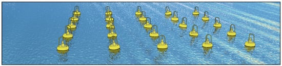
Figure 1.
Point absorber wave park comprising 25 identical floating devices.
The model proposed in the present work is developed based on linear theory and comprises a frequency domain BEM approach, supplemented by a Consistent Coupled Mode System (CMS) that models wave propagation over irregular bathymetry. Thus, the influence of fluid viscosity is not taken into account, which could cause important deviations at specific frequencies. Nevertheless, the 3D numerical approach based on boundary integral equations allows for the modeling of any WEC shape, as opposed to reduced 2D models, and can provide useful results in an extended range of frequencies and angles of incidence. In the context of the present work, we consider an array of single degree-of-freedom (DoF) point absorbers, with each unit being free to oscillate in heave alone, leading to a simplified hydrodynamic model, as compared to the full six DoF setup. As a result, the proposed model ignores the coupling between different degrees of freedom, which could lead to underestimation or overestimation on the response of certain units of the array at particular excitation frequencies. However, it is much more efficient in terms of computational requirements, as compared to the six DoF setup. The results concerning the response of the array can be used to assess the system performance on the basis of spectral average characteristics. In the existing literature, the effect of irregular bathymetry on the operation of wave energy parks has been investigated at a preliminary stage. More specifically, Ref. [13], investigates bathymetric effects on the far field of a WEC park, with the bathymetry profile, however, being constant in the vicinity of the WEC array. Additionally, in Ref. [7], the operation of WECs is studied over irregular bathymetry by a 2D model, that makes use of the MMSE. In the latter work, the point absorbers are modeled on the free surface plane as energy absorbing circular inclusions, while the absorption parameters are calibrated by local 3D BEM formulations in constant local depth. Τhe innovation of the present model lies in the inclusion of real bathymetric data in the modeling, along with oblique wave incidence on the WEC park, which allows for the quantification of the power absorption in site-specific cases, based on local seabed topography, combined with the local wave climate data.
2. Mathematical Formulation
We consider a WEC array of single degree-of-freedom (DoF) heaving point absorbers, comprising M identical devices, operating in some nearshore area where the seabed may present variations, while harmonic propagating incident waves stimulate the whole array. The response of each device in heave is obtained by modeling the surrounding field in the domain D (see Figure 2), accounting for the interaction of the field with the variable bathymetry, as well as intra-array interactions, as discussed in more detail in the sequel. In accordance with the standard hydrodynamic theory for floating structures, the overall flow field consists of the propagating field (incident and diffracted) and M radiation fields, generated by the devices’ motion. Each of the above is represented by a corresponding potential function , and , respectively, so that the resulting velocity fields are equal to . A Cartesian coordinate system is defined, whose origin is placed at Still Water Level (SWL), so that the waterplanes of the whole array are symmetric with respect to the and planes (see Figure 2). The number of WECs in the and -directions is and , respectively (thus, . In this work’s context, the submerged volume of each WEC consists of a cylindrical buoy of radius and draft , supplemented by an oblate semi-spheroidal part, with semi-major axis equal to and semi-minor axis equal to (see Figure 2 and Figure 3), leading to a total draft of . The unit vector, that is normal to the boundary and directed toward the exterior of , is denoted by (see Figure 2). The centers of the two adjacent WECs’ waterplanes are positioned apart in the -direction and apart in the -direction. Finally, the WEC numbering starts from the device, in the 3rd quadrant of the plane, which is the farthest from the origin (see Figure 2). The numbering continues along the -axis until the WEC and the next device is selected to be the one located in the next row of the park and whose waterplane’s midpoint shares the same -coordinate as the 1st device. The numbering is defined similarly until the M-th unit.
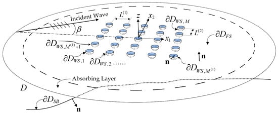
Figure 2.
Sketch of a WEC park comprising 25 floating devices, illustrating the flow Domain D and the parts of boundary , along with basic parameters.
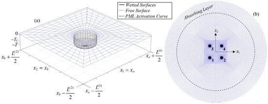
Figure 3.
(a) Indicative mesh of a WEC’s wetted surface, along with the corresponding free surface block’s mesh. (b) Mesh of a WEC park comprising 4 devices (top view), illustrating the WEC numbering and the PML activation curve.
Assuming that all time-dependent quantities oscillate harmonically in the form , where denotes the frequency in [rad/s] and is the imaginary unit, the problem is transferred to the frequency domain by the following representation:
In Equation (1), stands for the incident wave height, is the gravitational acceleration, is the complex amplitude of the m-th device’s response in heave, is the angle of incidence with respect to the -axis and is the total complex potential, which comprises all the subfields and is defined in the frequency domain as:
In Equation (2), and , respectively, stand for complex amplitudes of the incident and the diffracted subfields. Furthermore, is the complex amplitude of the radiation field generated by a unit-amplitude heaving oscillation of the m-th WEC.
2.1. Formulation of the Incident Field
The potential function of the incident field propagating over the seabed, is obtained by a consistent coupled mode model (CMS), free of mild bottom slope assumptions, as extended for three-dimensional environments in Ref. [14]. In the general case, the incident potential is obtained by splitting the function that expresses the depth variation into two components: , where is a parallel-contour bathymetry and denotes additional three-dimensional depth irregularities. The solution is accordingly split as .
In the framework of this work, considering that the isobaths are approximately parallel approaching the coastline, the depth function of the domain D exhibits a 1D variation (see Figure 2 and Figure 4b) of the form , connecting two regions of fixed but different depths, (incidence region) and (transmission region). The incident field is given by:
where is the incident wavenumber at depth , and is the angle of incidence over the parallel contour bathymetry . Substituting Equation (3) into the Laplace equation, the linear form of the free-surface boundary condition (BC) and the Neumann BC at the sea bottom, we obtain a corresponding boundary value problem (BVP) for the unknown potential , for the case of oblique-incident harmonic waves, which is supplemented by proper radiation conditions for the incidence and transmission regions [14]. This problem is solved utilizing a one-dimensional version of the CMS, where the potential accepts the local-mode representation:
In Equation (4), denotes the propagating mode, denotes the evanescent modes, and the term is an additional term, referred to as the sloping-bottom mode, which is introduced to satisfy the homogeneous Neumann BC on the sloping parts of the seabed. The eigenfunctions , which are obtained by local vertical Sturm–Liouville problems formulated in the local vertical intervals , represent the local vertical structure of the n-th mode and are given by:
where the eigenvalues , involved in the above expression, are obtained as the roots of the local dispersion relations,
with being the only real root and being the infinite series of imaginary roots of Equation (6). Utilizing the local-mode representation of Equation (4), a coupled-mode system is formulated for the horizontal complex amplitudes of the form,
where the definition of the coefficients and of the CMS is based on the vertical modes , which are spatially variable due to local depth dependence, see Ref. [14]. The system of Equation (7) is supplemented by appropriate BCs, extracted by matching the unknown potential with the solutions at the two semi-infinite strips of depth and , respectively. The sloping-bottom mode becomes important in the cases of local topographies with steep sloping parts and notably accelerates the convergence of the series of local modes, described by Equation (4); with four to six terms in total being enough to assess the incident field in areas characterized by seabed slopes of more than 100%; see Ref. [14] for more details. In the special case where only is kept, the model reduces to the modified mild-slope equation (MMSE) derived by Massel [15] in 1993 and by Chamberlain and Porter [16] in 1995.
2.2. BEM Formulation for the Diffraction and Radiation Problems
Boundary value problems (BVPs), with the Laplace equation for the potential functions being the field equation, supplemented by suitable boundary conditions (BCs) at the different sections that make up the boundary of the domain, are numerically solved to evaluate the diffraction and radiation fields. The latter boundary, as illustrated in Figure 2, comprises the water-free surface () the wetted surface of each device (, m = 1, 2,…, M) and the solid boundary of the seabed (). The mixed free surface boundary condition (FSBC) is used on and no-entrance BCs are used on the solid boundaries, resulting in the following BVPs,
In the above Equations, denotes the unit normal vector on , directed toward the exterior of the domain (also shown in Figure 2). In Equation (8d), is the Kronecker delta. According to the latter equation, the m-th radiation field is evaluated by applying a BC, which enforces a unitary heaving oscillation of the m-th WEC, while the rest of the devices are treated as being fixed at their mean position. The frequency parameter involved in the FSBC (Equation (8b)), is expressed as a function of the horizontal position , to account for modifications concerning the application of appropriate radiation conditions at infinity. Specifically, the wave fields computed as solutions to the above BVPs propagate undisturbed in directions , which implies that the flow domain extends infinitely. A perfectly matched layer (PML) technique (see Figure 2) is utilized to truncate the computational domain. The PML consists of an absorbing layer that is used to artificially weaken and ultimately zero-out the outgoing wave solutions, treating their radiating behavior at far distances from the WEC park; see also Ref. [4].
The layer’s thickness, which must be of the order of one local wavelength [4], determines the solution damping efficiency and the elimination of numerical reflections. In this work’s context, the layer thickness is selected to be equal to one mean wavelength , amplified by a factor of 15% to account for longer wavelengths at the deeper regions of the domain. denotes the root of the dispersion relation in the real axis, as defined at the mean depth of the area spanned by the WEC array. It is noted that the absorbing layer with the above characteristics was found to provide the sufficient solution damping at the deeper regions of the domain for the local topography studied in this work, which is analyzed in the sequel, as well as the studied frequency range. However, the layer thickness might need readjustment for lower frequencies and for areas with greater depth changes between deep and shallow regions. The PML technique is implemented by introducing an imaginary component to the frequency parameter in the layer:
where denotes the PML activation radius (see Figure 2). Optimum values of the parameters and , involved in Equation (9), are selected (see Ref. [4]) to increase the efficiency of the layer, with regard to the minimization of numerical reflections in the assessed solutions.
A low-order Boundary Element Method (BEM) scheme is developed to numerically solve the BVPs, described by Equation (8). The method involves simple singularity distributions on 4-node quadrilateral elements, while continuity of the geometry is ensured on the boundary parts and the junctions between them. The functions , are expressed as:
where is the Green’s function for the Laplace equation in three dimensions and are discrete strength distributions, defined on the panels that make up the boundary . The latter strength distributions are obtained by the BEM, given that they are defined as a piecewise constant. The distributions , combined with a discrete form of the integral representation (Equation (10)), define the involved subfields . In particular, the potentials and the velocity fields are approximated by,
where the summation index p covers all of the panels that model and are the strength of the singularity distribution, corresponding to the m-th subfield, on the p-th panel which is, in general, complex due to the non-zero imaginary part of the frequency parameter in the PML region. The induced quantities (potential and velocity) by the p-th element (carrying unitary distributed singularity) to the point x in the field are, respectively, denoted by and ; see e.g., Ref. [17]. Numerical solutions are obtained by satisfying each BC at the centroids of the panels distributed across the various boundary sections, using a collocation technique. Constant normal dipole distributions are used on the panels, and thus induced potential is analytically available using the solid angle; see Ref. [18]. Furthermore, induced velocity can be computed by the repetitive application of the Biot–Savart law, since a constant dipole element is equivalent to a vortex ring [17].
The mesh is generated by combining matching structured meshes of the distinct boundary surfaces, ensuring continuous junctions between the different segments which, in conjunction with the 4-node panels, result in global continuity of the discretized boundary. More specifically, the mesh of the WEC’s wetted surface consists of a part that models the lateral surface of the submerged volume’s cylindrical part, supplemented by a mesh of the oblate semi-spheroidal part, defined in spherical coordinates. Furthermore, the free surface in the vicinity of each WEC is modeled by a rectangular block of dimensions and , in the and -directions, respectively, centered at the WEC waterplane’s midpoint. The block is discretized by a radial mesh, using gradually increasing resolution while approaching the wetted surface, for obtaining better quality results. An indicative boundary mesh of a WEC, along with the corresponding free surface block mesh, is illustrated in Figure 3a. The computational mesh shown in Figure 3a is replicated M times to produce the mesh of the whole WEC park, as depicted in Figure 3b (for the case ). Subsequently, a radial mesh is constructed around the WEC park, modeling the remainder of the free surface boundary, extending to a certain number of mean wavelengths and thus, the total radius of the mesh as well as the activation radius of the PML are frequency dependent. It is noted that the nodes distributed in the azimuthal direction are doubled at a specific radius, as shown in Figure 3b, in order to maintain a predefined minimum of elements per wavelength (15–20) in both the angular and radial directions, at the outer part of the free surface mesh. The , coordinates of the seabed mesh in the area of the park are defined by a simple rectangular mesh, while the rest of the seabed boundary mesh is defined similarly to that of the free surface. The -coordinate can be used to model any arbitrary seabed topography.
After obtaining all of the involved subfields, the complex amplitudes of the devices’ response in heave ( are obtained as a solution to the following linear system:
In Equation (12), the diagonal matrix M = MI models the inertia of the heaving point absorbers, with being the identity matrix, being the mass of each device and ρ being the density of the water. Furthermore, hydrostatic restoring forces are represented in Equation (12) by the matrix , where is the hydrostatic restoring coefficient in heave. The energy extraction by the power take-off (PTO) system is modeled by a damping coefficient, denoted in Equation (12) by the diagonal matrix where , and is the stiffness of the PTO system. The added mass is model\led by an M × M matrix, whose elements are defined, for a given frequency, by the component of the radiation force, induced by the -th radiation field on the m-th WEC, that is in phase with the acceleration, while the corresponding elements of the M × M hydrodynamic damping matrix are evaluated by the component in phase with the velocity. The aforementioned force is computed via integration of the pressure induced by the -th radiation field on the m-th wetted surface, multiplied by the (vertical) component of the normal vector,
Furthermore, the pressure induced by the incident and the diffracted subfields, in conjunction with the vertical component of , is integrated on each wetted surface to determine the Froude–Krylov forces and the diffraction excitation forces on each WEC,
The mean power output by each device is subsequently defined as,
assuming there are no losses due to the PTO system. The normalized power , which is evaluated taking into account the intra-array interactions as well as the local bathymetry, is defined by dividing the mean power output with the incident power flux over a cross section equal to each device’s waterline diameter, and evaluated at the depth of the deep region (region of incidence). The latter incident power flux is used, since the wave amplitudes and wave numbers at the vicinity of each WEC may differ due to depth variations. Considering an incident wave of height at the region of incidence, equals,
where denotes the group velocity, calculated at the incidence region’s depth.
3. Case Study
We consider a WEC park consisting of twenty-five (25) devices, placed in a 5 × 5 arrangement, see Figure 4, operating at the north coast of the island of Ikaria, located in the Eastern Aegean Sea region, where the wave energy potential is relatively increased [19].
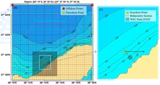
Figure 4.
(a) Computational grid for the application of SWAN and (b) local bathymetry at the north coast of Ikaria Island, indicating the considered WEC park position and the section that defines the local bathymetry of the BEM-CMS model. (* not to scale).
The wave climatology in the region is derived by a 10-year-long time series, which is obtained from the ERA5 database [20] and covers the period between the years 2013 and 2022, at the offshore points 37°45′ N, 26°10′ E and 37°45′ N, 26°20′ E (see Figure 4a). The significant wave height () and the mean energy wave period () are included in the available dataset, along with mean wave direction (—measured clockwise with zero at North), with a resolution in time. Nearshore wave parameters at the target point 37°39′05″N, 26°14′05″E, are obtained by an offshore-to-nearshore (OtN) transformation. The local depth at the target point is 40 m, (see Figure 4), which is also taken to be the maximum depth of the BEM-CMS model () at the region of incidence (see Equation (16)). The OtN is performed using the SWAN model, see [21]. Offshore conditions defined by the parameters ), are considered known, across the seaward boundary and are used to reconstruct directional spectra utilizing the JONSWAP spectrum, along with a hyperbolic type spreading function; (see Section 3.4.4 of Ref. [22]).
The bathymetry used for the OtN, is obtained from GEBCO [23] and the coastline data are extracted from the GMT–GSHHS database; see [24]. Considering that the isobath lines are approximately parallel approaching the coastline, the depth profile of the domain D is defined by a 1D section of the local bathymetry, parallel to the -axis of the BEM model (see Figure 2 and Figure 4b).
Distributed offshore conditions on the seaward boundary are the main forcing of the system. The phase-averaged model SWAN is used, based on the offshore data, to assess the wave parameters within the computational grid, using adequate spatial resolution, as illustrated in Figure 4.
The main equation applied in the SWAN model is the radiative transfer equation,
Equation (17) expresses action balance, with representing the wave action density, defined in terms of spectral density and frequency . The components denote propagation velocity in the physical space, while denote corresponding components in the Fourier space. Moreover, represents the source terms which include, among others, wind-generated wave growth, wave breaking-induced dissipation in deep and shallow water and bottom friction. The OtN transformation is discussed in more detail in Ref. [25]. Offshore wave climatology at the two offshore points, is presented in Figure 5, where the distributions are represented by standard lognormal and KDE models. The corresponding nearshore climatology is shown in Figure 6.
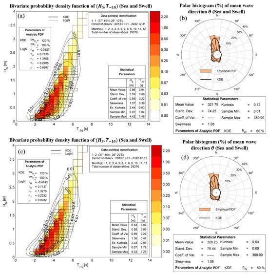
Figure 5.
Wave climatology at the offshore points (a,b) 37°45′ N, 26°10′ E and (c,d) 37°45′ N, 26°20′ E. (a,c) statistics and (b,d) corresponding polar histograms.
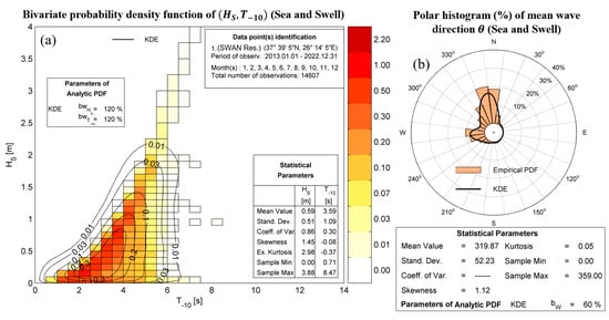
Figure 6.
Wave data at the target point with the geographical coordinates 37°39′05″ N, 26°14′05″ E and depth . (a) statistics and (b) corresponding polar histogram.
3.1. Application of the BEM-CMS Model
In order to efficiently implement the proposed BEM–CMS model, a parallel code was developed using MATLAB R2023a, for calculating the wave fields and the responses of the WEC array for a given frequency and the direction of incidence. The acquisition of the results presented and discussed in the sequel, for the studied ranges of frequencies and incidence directions, required a computing time of the order of 72 h on a workstation equipped with 192 GB RAM and two Intel Xeon Gold 6230R CPUs with 26 cores each. The studied frequency range corresponds to periods up to 10 s and the wavelength at the mean depth of the area spanned by the WEC array (), ranges from 7.6 m to 93.3 m. The total number of quadrilateral elements used for the computational mesh corresponding to the lowest frequency is 53,520, of which 21,600 on the twenty-five wetted surfaces, 19,920 on the free surface and the rest on the seabed boundary.
For higher frequencies, although the mesh radius decreases, maintaining a minimum number of elements per wavelength on the boundary of the free surface requires finer discretization, due to the constant spacing between the devices. For the case of the minimum wave period, the model used 63,740 elements, maintaining the size of the BEM influence matrix below 61 GB to meet memory limitations.
Figure 7 illustrates the real part of the propagating field (comprising the incident and the diffracted subfields), for the array of 25 WECs of radius , with total draft and , placed in a 5 × 5 arrangement with . The origin of the coordinate system of the BEM–CMS model is located 190 m away from the coastline and the local depth at is . All results hereafter refer to the above setup.
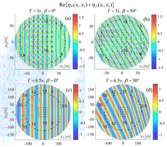
Figure 7.
Superposition of the incident and the diffracted subfields. Incident wave period (a,b) , (c,d) . Angle of incidence (a,c) , (b,d) . Dashed lines represent isobaths. The bold dashed line denotes the PML activation curve.
The color plots in Figure 7 illustrate the potential on the free surface, multiplied by so that it represents the free surface elevation . Figure 8 shows the real part of the free surface elevation corresponding to indicative radiation fields by the WECs 1 and 13. It can be observed that for low frequencies (see Figure 7c,d and Figure 8c,d), the interaction of the fields with the variable bathymetry becomes significant, while for higher frequencies (see Figure 7a,b and Figure 8a,b) the floating devices pose a more considerable effect on both the propagating and the radiated fields. The scattering in the downwave direction, which results in partial shadowing of waves at the lee side, is also observable in Figure 7a,b. Furthermore, the relevant reduction in the local wavelength can be seen in Figure 7c, which is triggered by the decrease in phase velocity due to an interaction of the field with the shoaling bathymetry. In the field shown in Figure 7d, the decrease in phase velocity also results in refraction, due to oblique wave incidence, and it can be observed that the wavefronts tend to align with the isobath lines.
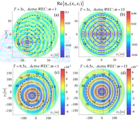
Figure 8.
Radiation fields by the WECs 1 (a,c) and 13 (b,d). Oscillation period (a,b) , (c,d) (equal to incident wave period). Dashed lines represent isobaths. The bold dashed line denotes the PML activation curve.
Figure 9 illustrates added mass contributions on WECs 1, 5, 13 and 25. The normalized added mass of an individual (isolated) WEC operating at the same region and located at (position of WEC 13 in the array), is also plotted for comparison. The elements of the added mass matrix are normalized using the mass of a WEC with the considered submerged volume, which is equal to , of which approximately 85.8% corresponds to the cylindrical part of the submerged volume and 14.2% to the oblate semi-spheroidal part with a semi-major axis equal to and a semi-minor axis equal to .
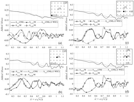
Figure 9.
Normalized added mass contributions on WECs (a) 1 (b) 5 (c) 8 and (d) 14. The normalized added mass of an individual WEC operating at the same region and located at (position of WEC 13 in the array), is also plotted for comparison. Relative position of the WECs is illustrated in the auxiliary legend.
As it can be seen in Figure 9b, the elements and of the added mass matrix present almost identical behavior due to the symmetry of the relevant position of the corresponding devices on the plane. However, minor differences are observed at the low frequency range, which are triggered by the seabed profile. This effect is also evident in Figure 9c, as regards the added mass contributions of the WECs 6 and 10 on WEC 8. On the other hand, the elements and of the added mass matrix behave identically (see Figure 9d), since not only are the relevant positions of these devices symmetric on the plane, but also the devices 4 and 24 are positioned over the same isobath line.
Corresponding results concerning the hydrodynamic damping are illustrated in Figure 10. The hydrodynamic damping data are made non-dimensional by normalizing, with respect to the mass of a WEC times the angular frequency. The bathymetry induced effects are also observable in the hydrodynamic damping data.
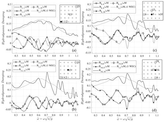
Figure 10.
Normalized hydrodynamic damping contributions on WECs (a) 1 (b) 13 (c) 8 and (d) 14. The normalized damping of an individual WEC operating at the same region and located at (position of WEC 13 in the array), is also plotted for comparison. Relative position of the WECs is illustrated in the auxiliary legend.
Non-dimensional forces acting on WECs 1, 5, 13 and 25 (normalized by , where A is the amplitude of the incident field at the region of incidence), are shown in Figure 11, for incidences normal to the depth contours and for . The figure shows both the Froude–Krylov (FK) and diffraction forces. Corresponding results concerning an individual (isolated) WEC operating at the same region and located at (position of WEC 13 in the array), are also shown for comparison. It can be observed that the FK forces acting on WEC 13 exactly match those acting on the isolated device, while the FK forces on the other WECs present minor differences, depending on the local depth of where they are located. The diffraction forces present more complicated patterns due to intra-array interactions. As it can be seen in Figure 11c, the diffraction forces acting on the WECs 5 and 25 are identical in the case of wave propagation normal to the depth contours, due to symmetry. This applies to any two devices positioned symmetrically, with respect to the plane for .
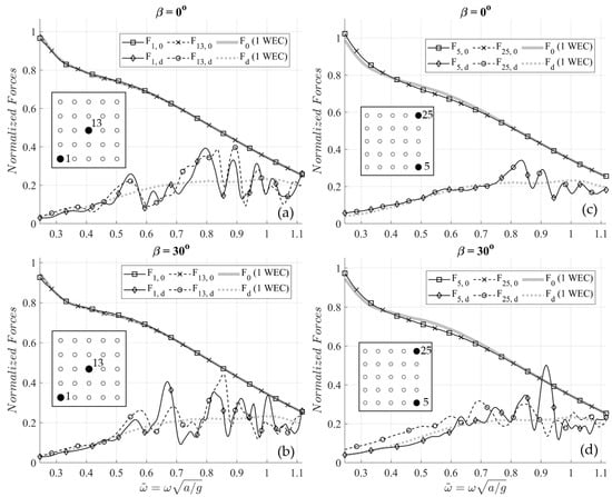
Figure 11.
Normalized Froude–Krylov and diffraction forces on WECs (a,b) 1 and 13, (b,d) 5 and 25. Propagation direction (a,c) and (b,d) . The normalized Froude–Krylov and diffraction forces acting on an individual WEC operating at the same region and located at (position of WEC 13 in the array), are also plotted for comparison. Relative position of the WECs is illustrated in the auxiliary legend.
Response amplitude operators (RAOs) of the WECs 1, 13 and 25 are illustrated in Figure 12, as computed by Equation (12) for . The PTO stiffness is set to 10% of the hydrostatic restoring coefficient (), corresponding to magnitudes used in the literature [26] and the PTO damping is defined as , where is the mean hydrodynamic damping of an individual (isolated) WEC operating in the under-study region (see Figure 10—gray lines) and is a multiplying factor. Based on the above, the PTO damping parameter is approximately equal to .
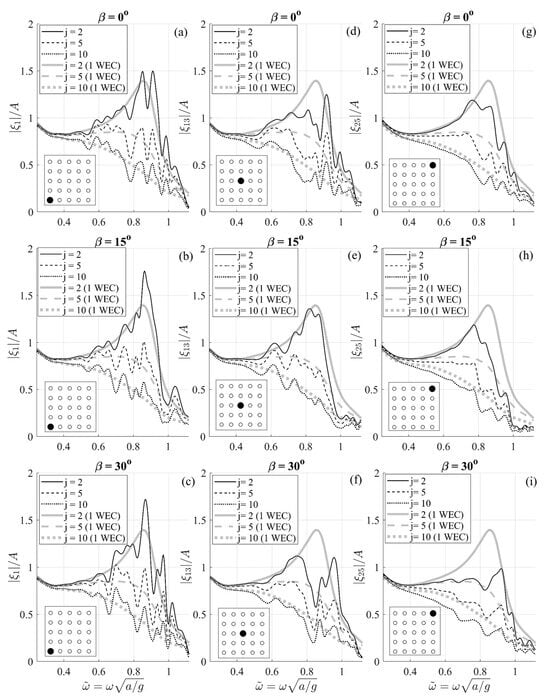
Figure 12.
Normalized responses of WECs (a–c) 1, (d–f) 13 and (g–i) 25. Propagation direction (a,d,g) , (b,e,h) , (c,f,i) . The normalized responses of an individual WEC operating at the same region and located at (position of WEC 13 in the array) are also plotted for comparison. The relative position of the WECs is illustrated in the auxiliary legend. , .
Corresponding results concerning the isolated WEC are also shown for comparison.
As it can be seen in Figure 12, devices with which a wavefront interacts first exhibit increased responses, due to the presence of reflected wave components in their vicinity, generated by the rest of the array. On the other hand, the WECs located at the downwave region experience the shadowing of the wave field due to the preceding devices, and thus perform oscillations of reduced magnitude. This difference in response magnitude is apparent by comparing the responses of WECs 1 and 25 in the case where the incident field propagates at see Figure 12c,i.
Figure 13 depicts the normalized power output by the same WECs (1, 13 and 25) for different values of the multiplying factor , as computed by Equation (16) for . Results concerning the isolated WEC are also plotted for comparison. The above observation concerning the response amplitude operators also holds for the normalized power curves, since the RAO values are explicitly involved in the calculations. The fact that the devices that first encounter the wavefronts benefit from intra-array interactions also agrees with the findings reported in Ref. [27]. Furthermore, as illustrated in Figure 13, the higher the value of PTO damping, the better the devices perform at the low frequencies range.
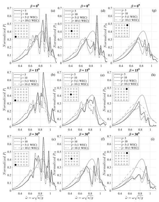
Figure 13.
Normalized power output by the WECs (a–c) 1, (d–f) 13, and (g–i) 25. Propagation direction (a,d,g) , (b,e,h) , (c,f,i) . The power output by an individual WEC operating at the same region and located at (position of WEC 13 in the array), is also plotted for comparison. The relative position of the WECs is illustrated in the auxiliary legend. , .
The -factor is an index that quantifies the effect of hydrodynamic interactions between the devices, on the power absorption of the whole system, and was first introduced in the late 1970s [28]. It is defined as the ratio of the power generated by an array comprising M devices, to M times the power generated by an isolated device. Therefore, implies that the average power output per WEC of the array is reduced, compared to that of the isolated WEC and thus the interactions have a negative impact on the overall power absorption, while q > 1 means that the interactions act constructively [27].
The q-factor of the considered arrangement, defined as,
is shown in Figure 14, for different levels of the angle of incidence and for different values of the multiplying factor , including the value , ( = 35.14 kN/s) which was found to be the optimum, as regards the maximization of the mean annual power output of this arrangement in the considered geographical region, as analyzed in more detail in the sequel. In Equation (18), denotes the normalized power output by the m-th WEC of the 5 × 5 array, for the given parameters, and is the normalized power output by the isolated WEC operating at the same region and located at . It can be observed that in the low frequency range, the intra-array interactions are negligible (and thus the -factor is approximately one) while for higher frequencies the -factor presents more complicated behavior, that is highly dependent on the angle of incidence, and less sensitive to changes in the PTO damping . The value of required to optimize the annual power output is a consequence of the selected devices’ low-natural period in heave as compared to the sea states with the higher energy content in the considered region. Furthermore, the natural period is further slightly reduced by the considered PTO stiffness. Apparently, more massive devices would require less PTO damping. However, in this work’s context the studied devices were chosen to measure three meters in diameter, so that the presented results would be comparable to practical applications [29]. In the general case, a simple estimation of optimum mass and diameter values (that maximize the responses of freely floating bodies—and assuming that and ) could be determined by adjusting the natural period of WECs in heave motion to approach the value of the period carrying the biggest amount of energy in the region, based on the nearshore wave climate data; see Figure 6 (which is usually slightly larger than the mean wave period, due to a positive correlation between the energy period and the significant wave height).
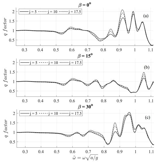
Figure 14.
5 × 5 WEC arrangement -factor for different PTO damping values. Propagation direction (a) , (b) , (c) , .
A colorplot of the q-factor is shown in Figure 15, for angles of incidence in the range [], for the optimum value of PTO damping. The sections shown in Figure 14 are denoted by dashed lines in the colorplot.
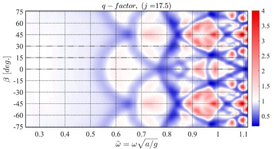
Figure 15.
-factor of the 5 × 5 WEC arrangement. Propagation direction , , .
3.2. Estimation of Absorbed Power
The TMA model [30] is used to reconstruct the wave spectra based on the time series of nearshore wave data:
where is the JONSWAP spectrum and is the TMA filter function. Every spectrum of the series, constructed by Equation (19), is discretized into a large number of frequencies ( is the frequency spacing), and all energy is considered to be concentrated in the mean direction . The WEC arrangement is oriented towards the northwest and specifically at 319 degrees; see Figure 4b. Thus, in the case of incident fields coming from this azimuthal direction, the absorbed power by the WEC park is evaluated using the results of the BEM–CMS model for . Given the arrangement symmetry with respect to the -plane, the power curves for , are used to estimate power absorption by indent spectra with . The power output of the 25-WEC system, for each spectrum , is estimated as follows:
where and represent the normalized power output of the m-WEC, for the given parameters. Polar histograms of net incident and absorbed wave power are shown in Figure 16.
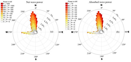
Figure 16.
Polar histograms (%) of (a) net incident wave power and (b) absorbed wave power by the 5 × 5 WEC arrangement. , .
Figure 17 shows a 10-year-long time series of the calculated power output by the considered 5 × 5-WEC arrangement, operating north of the coast of Ikaria Island for , which was found to be the value that maximizes the mean power production, for the considered fixed value. The system’s mean power output is 15.29 kW, which translates to 134.03 MWh produced on an annual basis. The power output ranges from 0 kW to a maximum of 289.84 kW. The probability density function of the annual absorbed power is illustrated in Figure 18a, while Figure 18b–e illustrates corresponding seasonal data. The data presented in Figure 16, Figure 17 and Figure 18 are obtained using results of the BEM-CMS model with a 2-degree resolution in the angle of incidence starting from . Thus, the normalized power curves used for spectra with , are approximated by the power curves corresponding to
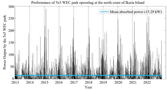
Figure 17.
10-year-long time series of power output (in kW) by the considered 5 × 5-WEC arrangement. , .
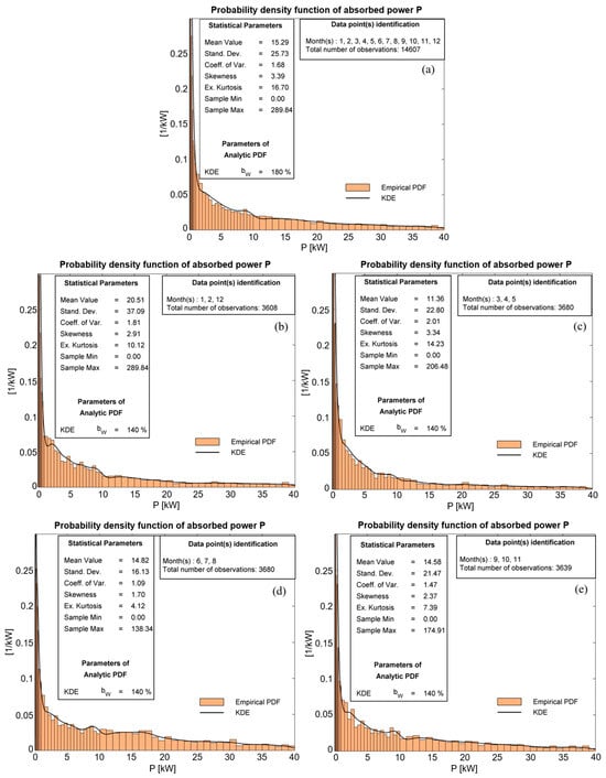
Figure 18.
The probability density function of (a) annual and (b–e) seasonal absorbed wave power by the considered 5 × 5-WEC arrangement. (b) Winter, (c) Spring, (d) Summer, (e) Autumn. , .
4. Conclusions
In this work, a methodology comprising a 3D BEM and a CMS model is developed and discussed to evaluate the energy-capturing capacity of a WEC array, consisting of several floating-point absorber WECs, accounting for intra-array interactions, as well as interactions with the local seabed topography and oblique-wave incidence. A case study is presented for a selected nearshore site, north of the coast of Ikaria Island, located in the Eastern Aegean Sea region, using long-term climatological data as obtained by an OtN transformation. The study illustrates the applicability of the proposed method as a tool for the optimal design of the WEC layout. Numerical results are displayed regarding various quantities of interest, including the exerted forces on selected devices of the array, indicative elements of the hydrodynamic damping and added mass matrices, as well as the effect of PTO parameters on the responses and the power output. In addition, indicative flow fields are presented and discussed, highlighting the effectiveness of the model in simulating refraction/diffraction phenomena. The park effect (-factor) is also quantified and presented for the studied arrangement. Recent studies have shown that installing devices with different individual dimensions within a park can improve the overall performance [31], which will be investigated in future studies using the current methodology, along with different shapes and arrangements of the devices, aiming for the maximization of the power output. The performance of floating WECs could be enhanced by the consideration of additional degrees of freedom [32] and the first results in this direction have been presented in [33]. In this case, the coupling between different DoFs could result in large-amplitude angular oscillations of the WECs [34], which can prove to be an additional important design parameter, as regards the survivability of the devices in harsh conditions.
Author Contributions
Conceptualization, T.G.; methodology, T.G., A.M., K.B.; software, T.G., A.M.; validation, A.M., T.G.; writing—original draft preparation, T.G., A.M.; writing—review and editing, T.G., A.M., K.B.; supervision, K.B. All authors have read and agreed to the published version of the manuscript.
Funding
This research received no external funding.
Institutional Review Board Statement
Not applicable.
Informed Consent Statement
Not applicable.
Data Availability Statement
Data are contained within the article.
Acknowledgments
The doctoral studies of A. Magkouris have been supported by the Special Account for Research (E.L.K.E.) of the National Technical University of Athens (NTUA).
Conflicts of Interest
The authors declare that there are no conflicts of interest.
References
- Guo, B.; Ringwood, J.V. A review of wave energy technology from a research and commercial perspective. IET Renew. Power Gener. 2021, 15, 3065–3090. [Google Scholar] [CrossRef]
- Babarit, A. Ocean Wave Energy Conversion, 1st ed.; ISTE Press-Elsevier: Amsterdam, The Netherlands, 2017. [Google Scholar]
- Stratigaki, V.; Troch, P.; Stallard, T.; Forehand, D.; Kofoed, J.P.; Folley, M.; Benoit, M.; Babarit, A.; Kirkegaard, J. Wave Basin Experiments with Large Wave Energy Converter Arrays to Study Interactions between the Converters and Effects on Other Users in the Sea and the Coastal Area. Energies 2014, 7, 701–734. [Google Scholar] [CrossRef]
- Belibassakis, K.; Bonovas, M.; Rusu, E. A Novel Method for Estimating Wave Energy Converter Performance in Variable Bathymetry Regions and Applications. Energies 2018, 11, 2092. [Google Scholar] [CrossRef]
- Charrayre, F.; Peyrard, C.; Benoit, M.; Babarit, A. A coupled methodology for wave body interactions at the scale of a farm of wave energy converters including irregular bathymetry. In Proceedings of the 33rd Intern Conference on Offshore Mechanics and Arctic Engineering (OMAE2014), San Francisco, CA, USA, 8 June 2014. [Google Scholar]
- Li, Y.; Yu, Y.H. A synthesis of numerical methods for modeling wave energy converter-point absorbers. Renew. Sust. Energ. Rev. 2012, 16, 4352–4364. [Google Scholar] [CrossRef]
- Bonovas, M.; Magkouris, A.; Belibassakis, K. A Modified Mild-Slope Model for the Hydrodynamic Analysis of Arrays of Heaving WECs in Variable Bathymetry Regions. Fluids 2022, 7, 183. [Google Scholar] [CrossRef]
- Gao, J.; Zang, J.; Chen, L.; Chen, Q.; Ding, H.; Liu, Y. On hydrodynamic characteristics of gap resonance between two fixed bod-ies in close proximity. Ocean Eng. 2019, 173, 28–44. [Google Scholar] [CrossRef]
- Gao, J.L.; He, Z.; Huang, X.; Liu, Q.; Zang, J.; Wang, G. Effects of free heave motion on wave resonance inside a narrow gap between two boxes under wave actions. Ocean Eng. 2021, 224, 108753. [Google Scholar] [CrossRef]
- Gao, J.; Gong, S.; He, Z.; Shi, H.; Zang, J.; Zou, T.; Bai, X. Study on Wave Loads during Steady-State Gap Resonance with Free Heave Motion of Floating Structure. J. Mar. Sci. Eng. 2023, 11, 448. [Google Scholar] [CrossRef]
- Bhinder, M.; Babarit, A.; Gentaz, L.; Ferrant, P. Effect of viscous forces on the performance of a surging wave energy converter. In Proceedings of the 22nd International Conference on Ocean, Offshore and Artic Engineering (ISOPE2012) hal-01202082f, Rhodes, Greece, 17–22 June 2012. [Google Scholar]
- Bhinder, M.; Babarit, A.; Gentaz, L.; Ferrant, P. Potential time domain model with viscous correction and CFD analysis of a generic surging floating wave energy converter. Int. J. Mar. 2015, 10, 70–96. [Google Scholar] [CrossRef]
- Verao Fernandez, G.; Balitsky, P.; Stratigaki, V.; Troch, P. Coupling Methodology for Studying the Far Field Effects of Wave Energy Converter Arrays over a Varying Bathymetry. Energies 2018, 11, 2899. [Google Scholar] [CrossRef]
- Belibassakis, K.A.; Athanassoulis, G.A.; Gerostathis, T.P. A coupled-mode model for the refraction-diffraction of linear waves over steep three-dimensional bathymetry. Appl. Ocean. Res. 2001, 23, 319–336. [Google Scholar] [CrossRef]
- Massel, S. Extended refraction-diffraction equation for surface waves. Coast. Eng. 1993, 19, 97–126. [Google Scholar] [CrossRef]
- Chamberlain, P.G.; Porter, D. The modified mild-slope equation. J. Fluid Mech. 1995, 291, 393–407. [Google Scholar] [CrossRef]
- Katz, J.; Plotkin, A. Low Speed Aerodynamics; McGraw-Hill: San Francisco, CA, USA, 2001. [Google Scholar]
- Newman, J. Distributions of sources and normal dipoles over a quadrilateral panel. J. Eng. Math. 1986, 20, 113–126. [Google Scholar] [CrossRef]
- Soukissian, T.; Gizari, N.; Chatzinaki, M. Wave Potential of the Greek Seas; WIT Transactions on Ecology and the Environment; WIT Press: Billerica, MA, USA, 2011. [Google Scholar]
- Dee, D.P.; Uppala, S.M.; Simmons, A.J.; Berrisford, P.; Poli, P.; Kobayashi, S. The ERA-Interim reanalysis: Configuration and performance of the data assimilation system. Q. J. R. Meteorol. Soc. 2011, 137, 553–597. [Google Scholar] [CrossRef]
- Booij, N.; Ris, R.C.; Holthuijsen, L.H. A third-generation wave model for coastal regions: 1. Model description and validation. J. Geophys. Res. Ocean 1999, 104, 7649–7666. [Google Scholar] [CrossRef]
- Massel, S.R. Ocean Surface Waves: Their Physics and Prediction. In Advanced Series on Ocean Engineering, 2nd ed.; World Scientific: Singapore, 2013; Volume 36. [Google Scholar]
- GEBCO Compilation Group (2023). GEBCO 2023 Grid. Available online: https://www.bodc.ac.uk/data/published_data_library/catalogue/10.5285/f98b053b-0cbc-6c23-e053-6c86abc0af7b/ (accessed on 20 January 2024).
- Wessel, P.; Smith, W. A global, self-consistent, hierarchical, high-resolution shoreline database. J. Geogr. Res. 1996, 101, 8741–8743. [Google Scholar] [CrossRef]
- Athanassoulis, G.A.; Belibassakis, K.A.; Gerostathis, T.P. The POSEIDON nearshore wave model and its application to the prediction of the wave conditions in the nearshore/coastal region of the Greek Seas. Glob. Atmos. Ocean Syst. 2002, 8, 201–217. [Google Scholar] [CrossRef]
- Anderlini, E.; Forehand, D.; Bannon, E.; Xiao, Q.; Abusara, M. Reactive control of a two-body point absorber using reinforcement learning. Ocean Eng. 2018, 148, 650–658. [Google Scholar] [CrossRef]
- Babarit, A. On the park effect in arrays of oscillating wave energy converters. Renew. Energy 2013, 68, 68–78. [Google Scholar] [CrossRef]
- Budal, K. Theory of absorption of wave power by a system of interacting bodies. J. Ship Res. 1977, 21, 248–253. [Google Scholar] [CrossRef]
- Jouybari, M.B.; Xing, Y. A practical design procedure for initial sizing of heaving point absorber wave energy converters. IOP Conf. Ser. Mater. Sci. Eng. 2021, 1201, 012018. [Google Scholar] [CrossRef]
- Massel, S. Hydrodynamics of Coastal Zones; Elsevier: Amsterdam, The Netherlands, 1989. [Google Scholar]
- Göteman, M.; Giassi, M.; Engström, J.; Isberg, J. Advances and Challenges in Wave Energy Park Optimization—A Review. Front. Energy Res. 2020, 8, 26. [Google Scholar] [CrossRef]
- Falnes, J. Ocean Waves and Oscillating Systems: Linear Interactions Including Wave Energy Extraction; Cambridge University Press: Cambridge, UK, 2004. [Google Scholar]
- Bonovas, M.; Belibassakis, K.; Rusu, E. Multi-DOF WEC Performance in Variable Bathymetry Regions Using a Hybrid 3D BEM and Optimization. Energies 2019, 12, 2108. [Google Scholar] [CrossRef]
- Tarrant, K.; Meskell, C. Investigation on parametrically excited motions of point absorbers in regular waves. Ocean Eng. 2011, 111, 67–81. [Google Scholar] [CrossRef]
Disclaimer/Publisher’s Note: The statements, opinions and data contained in all publications are solely those of the individual author(s) and contributor(s) and not of MDPI and/or the editor(s). MDPI and/or the editor(s) disclaim responsibility for any injury to people or property resulting from any ideas, methods, instructions or products referred to in the content. |
© 2024 by the authors. Licensee MDPI, Basel, Switzerland. This article is an open access article distributed under the terms and conditions of the Creative Commons Attribution (CC BY) license (https://creativecommons.org/licenses/by/4.0/).