Turbulent Characteristics of a Submerged Reef under Various Current and Submergence Conditions

Abstract

Submerged Reefs (SRs) are a kind of artificial fish habitat that can protect coasts and maintain ecological biodiversity. In this study, the flow field of the SR is simulated by solving a Reynolds-averaged Navier–Stokes equation closed with the Realizable k-ε model based on the finite volume method. The turbulent characteristics of SRs under different inflow velocities and submergences in the vicinity of the SR are analyzed. The wake vorticities are the primary turbulent pattern within and around the SR. The back wake and vorticity are chosen as critical indicators to quantitatively assess the hydrodynamic characteristics induced by the SR. The results show: (1) as the main flow passes through the SR, the upwelling is produced in front of the SR and a large-scale wake region is formed behind the SR which contains a clockwise vortex; (2) the length of the wake region formed behind the SR is positively and linearly correlated with both the inflow velocity and submergence; (3) the dipole-type vorticity patterns are induced within the compartment of the SR, where the area and average value of high vorticity have a positive correlation with the flow velocity and a negative correlation with the submergence, respectively.

1. Introduction

Global climate change, natural habitat degradation, and coastal erosion are accelerating coastal ecosystems’ deterioration worldwide. The Submerged Reef (SR) is a kind of artificial reef deployed on the sea bed, which can cause hydrodynamic changes within itself and in the surrounding sea area through changing the original marine geomorphology and flow field structure. The SR forms a benthic system to boost the populations of aquatic organisms by emulating the traits of natural habitats such as coral reefs [1,2,3]. Many studies indicate that fish tend to congregate around reefs due to the favorable conditions provided by wake flow [4,5,6]. Furthermore, the construction of the SR promotes waves breaking ahead, decreases wave transmission, and weakens wave energy nearshore, so as to protect coasts from severe erosion [7,8,9,10,11,12,13,14,15,16,17]. In short, the SR can alleviate the decline of fishery resources, enhance the population of marine organisms, protect coastal ecological environments, and alleviate coastal erosion [17,18,19,20,21]. The study of the flow structure both inside and outside the SR is of great importance for guiding practical ocean engineering.

The seafloor topography undulation caused by SRs combined with their inside structure form a complex flow field [22,23,24]. The water flows pass through the SR, bringing about a significant upwelling above the SR crest. Upwelling is defined as water rising from beneath the surface to replace water that has been pushed away. Furthermore, the interaction between the SR and the mainstream produces a wake behind the SR, i.e., back wake [25,26]. In particular, the upwelling transports nutrients from the bottom to the vicinity of the free surface [27,28,29,30], while the back wake promotes the deposition of nutrients in the rear of the SR [1], leading to the enhancement of water exchange [2]. Zooplankton, pelagic swimming organisms, and benthic resources are augmented by food supply and habitat modification due to the cycling of materials in the watershed [30,31,32]. Meanwhile, small-scale wakes and turbulence are generated inside the SR, forming an internal low-velocity but intense turbulence area owing to its perforated structural characteristics [33]. Due to the strong connectivity between the water bodies both inside and outside the SR, the internal turbulent flow directly affects the external flow regime, especially the formation of the back wake, which plays a vital role in hydrodynamic behavior and material transport [34,35,36]. The formation of small-scale turbulence within the SR can increase the growth and survival rates of fish larvae and enhance ecosystem stability [24,26]. Fischer et al. [37] noted that the turbulent intensity of the high Reynolds number turbulence is generated within the SR, which is strongly correlated with fish abundance (an indicator of fish fattening). Based on the RANS model using OpenFoam V. 1812^®, Hashempour and Kolahdoozan [38,39] carried out a numerical simulation study on the flow characteristics and sediment distribution with a porous three-dimensional tubular reef. The results show that a pair of reverse vortices are formed within the back wake in the vertical flow field.

When it comes to the flow field inside the SR, a vortex dipole is formed by the close pairing of two vortices of equal strength but opposite directions [40,41]. The formation of vortex dipoles plays an important role in the flow field by causing fluids’ mixture and diffusion, affecting the substances’ transport and exchange, and generating turbulence to promote flow energy dissipation [42]. Zheng et al. [33] conducted a fine experimental study on the turbulent structure inside a porous box SR using Particle Image Velocimetry (PIV). The study found that a pair of high-vorticity dipole vortex structures was formed inside the SR, which was induced by the jet-like effect of inflow from opening holes on the stoss face. Hence, it plays an important role in the mixing and exchange of the water inside and outside the SR. Due to the complexity of the structure itself, the turbulent pattern within the SR contains highly nonlinear turbulent processes, such as fluid separation and vortex evolution, which are difficult to solve analytically but are crucial for the accurate evaluation of the flow field effect in the SR [43]. Most of the studies on the flow field of underwater permeable structures, such as submerged reefs, focused on the upwelling and the back wake. However, there is a relative paucity of research on the turbulent characterization inside SRs.

It is quite necessary to examine the turbulent patterns within SRs under different inflow and submergence conditions, especially the generation and influence mechanism of inner vortical structure. In this study, numerical modelling validated with experimental data is carried out to analyze and discuss the turbulent characteristics within and around the SR affected by various inflow velocities and water depths.

2. Materials and Methods

The main aim of this section is to construct a numerical flume model using Computational Fluid Dynamics and validate this using experimental data. In actual practice, the flow field in the vicinity of the SR is nonlinear turbulence, which performs spatially irregular and temporally disordered fluid motion. To describe accurately the turbulence characteristics induced by the SR, the turbulence model chosen is crucial and critical for numerical prediction. Referring to previous research [33], the Reynolds-averaged Navier–Stokes equation closed by the Realizable k-ε turbulence model is an available and effective option for predicting turbulence detail for certain kinds of perforated reef-type breakwater, i.e., SRs. Limited by the length of this paper, the theoretical background of the numerical model is not presented here; however, the related content and the realization of the model are fully described in the user manual of ANSYS FLUENT 17.0 [44].

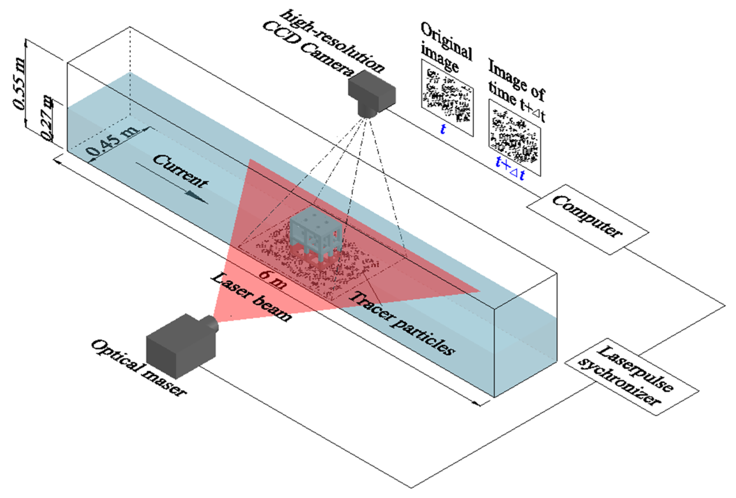
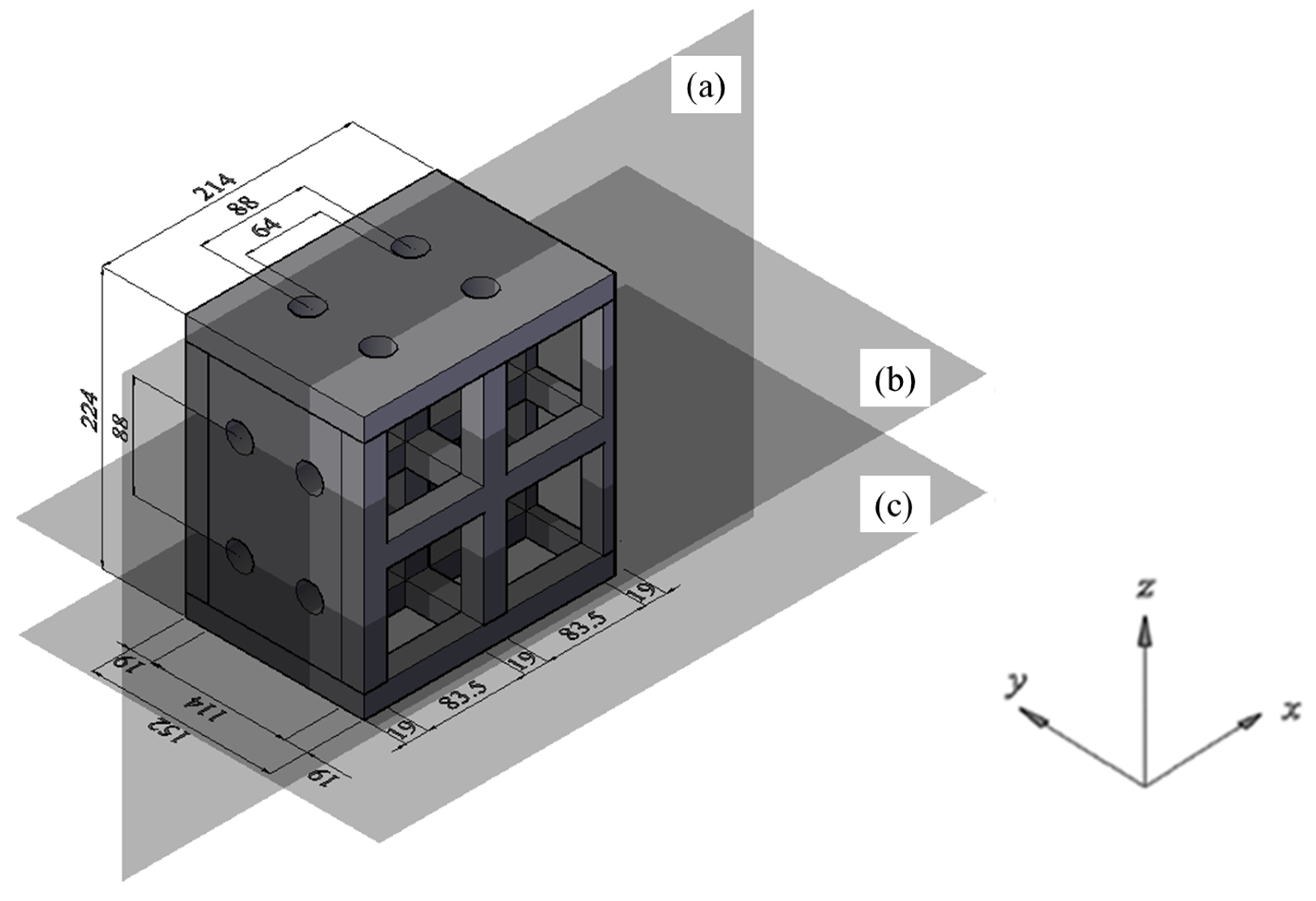
2.1. Experiment Setup

To verify the feasibility and accuracy of the numerical results, the turbulent flow field of the SR unit was measured using the Particle Image Velocimetry (PIV) technique at the Hydrodynamics Laboratory of Shanghai Ocean University, China. The experimental flume was 6.00 m long, 0.45 m wide, and 0.55 m high. Both the bottom and side walls of the flume were made of tempered glass, which made it easy to perform the PIV flow measurements, as shown in Figure 1. The SR model was designed according to the prototype deployed in the Beidaihe nourishment project in China. Based on the water depth of the Beidaihe coast and the experimental flume’s size, the scale model was 1:12.5 of the prototype to satisfy the flume’s physical constraints and the water depth was set at 0.27 m correspondingly. The SR model material was acrylic Plexiglas with a light transmission rate of 92%. The SR model had a length of L = 0.214 m, a width of B = 0.152 m, and a height of H = 0.224 m, and contained four circular holes with a diameter of 0.024 m in both the crest and stoss faces, as shown in Figure 2. Three profiles (vertical profile, transversal profile near crest layer, and transversal profile near bottom layer) were selected to present the three-dimensional turbulent characteristics. Further detail can be observed in [33]. The SR location, water depth, and inflow velocity were constant during the experiment.

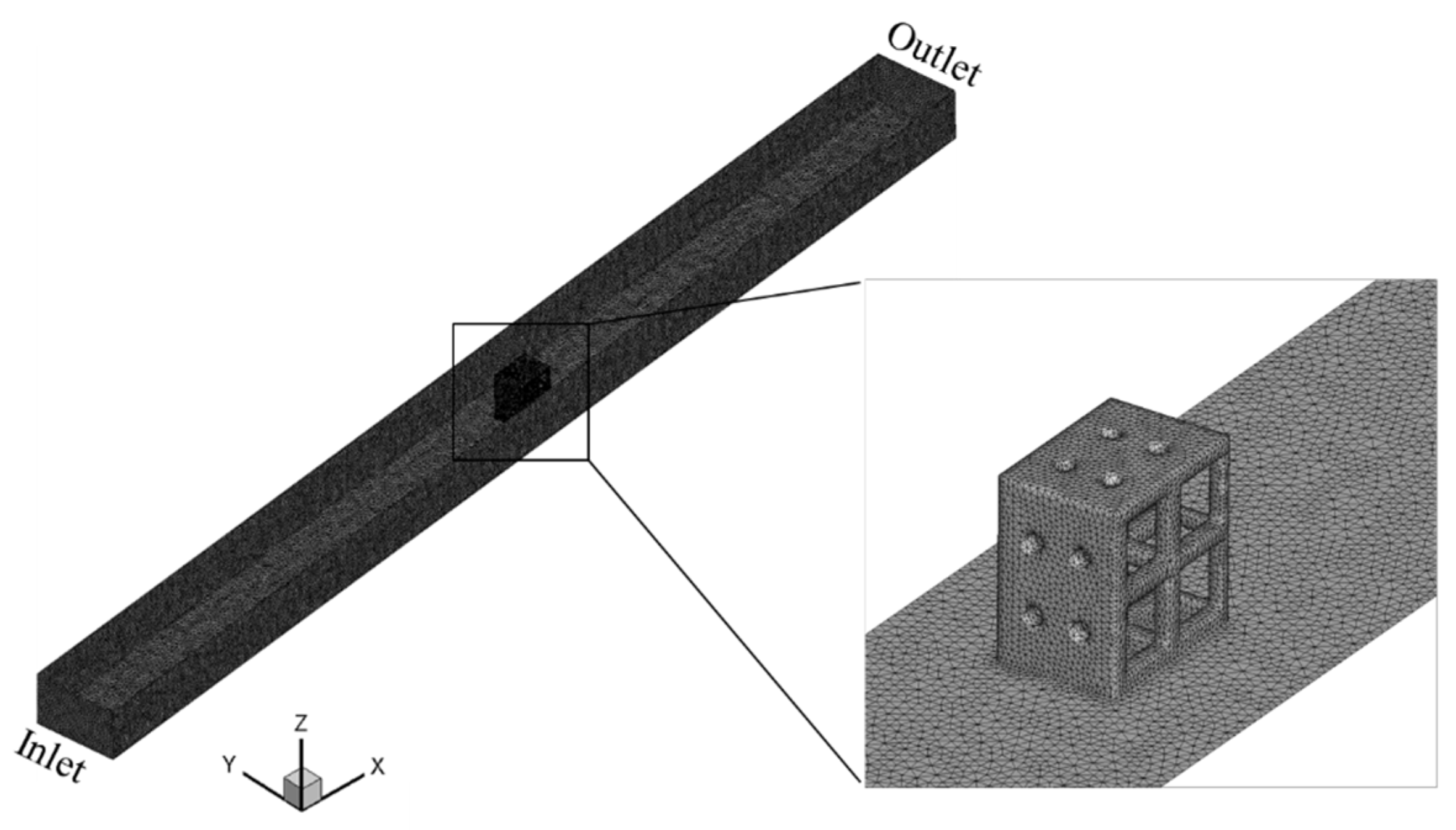
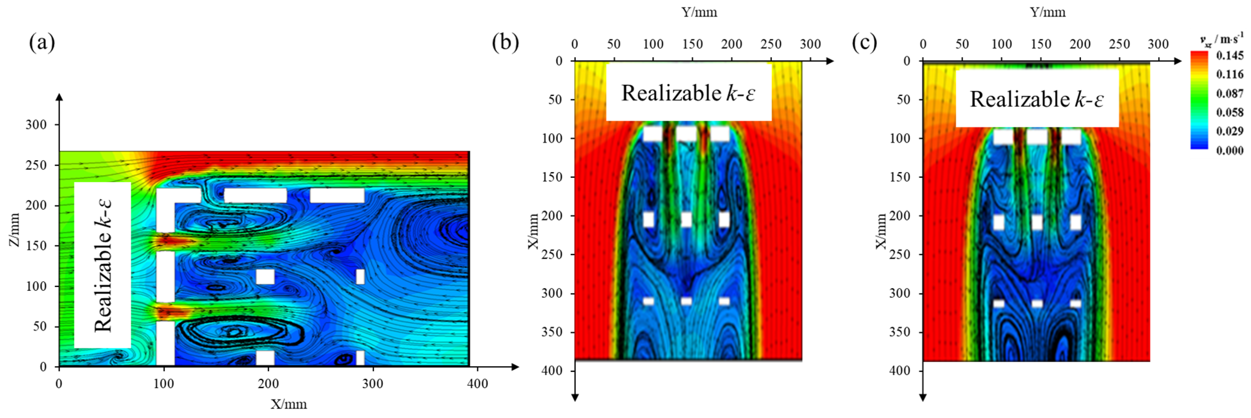
2.2. Numerical Model Setup

Considering the complex structure of the SR and the small-scale circular holes on the surface, the numerical model is discretized by the unstructured grid of tetrahedral cells. For validation, the model scales and specifications used in the numerical flume are consistent with those in the PIV experiment. The computational domain width and height are in accordance with the physical flume, while the length is set to 16 times the SR’s length (5 times in front of the SR and 10 times behind the SR) to ensure that the development of the wake region behind the SR could reach 10 times the SR’s length.

The boundary conditions are, respectively, set for the inlet, outlet, and wall. The outlet is modeled as a zero-pressure boundary condition, where unknown velocities are calculated from the incoming flow. The wall surface of the flume and the SR is prescribed as the stationary no-slip boundary condition. The free water surface is simulated as a moving wall with zero shear stress and the same inflow velocity. Based on the grid independence verifications, the model with a grid consisting of $112\times {10}^4$ elements is applied in the current numerical simulation to balance the accuracy and efficiency of the calculation, the detailed grid is shown in Figure 3.

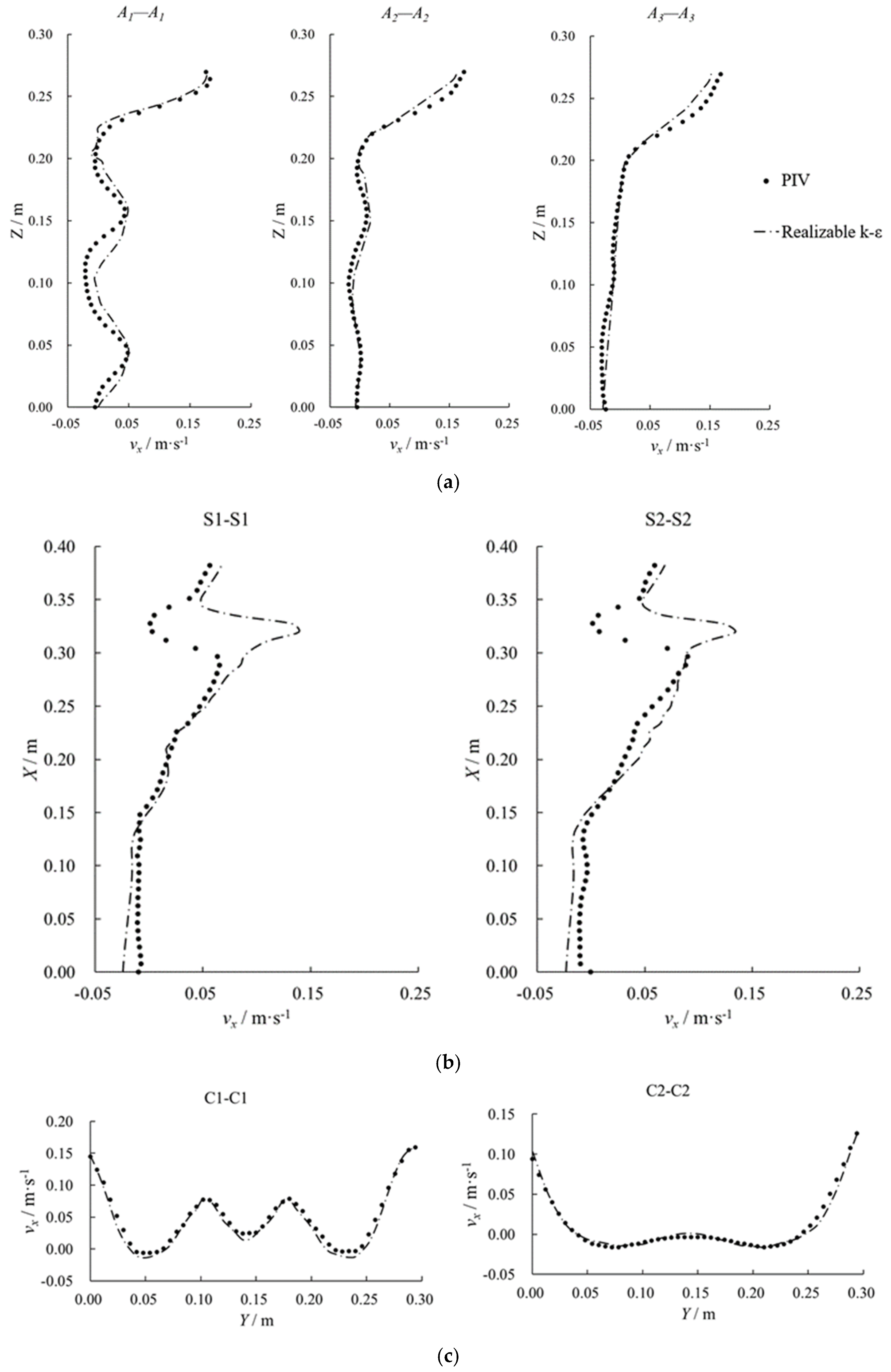
2.3. Model Validation

To examine the accuracy of the turbulence models, the longitudinal velocities in specific profiles are compared between experimental and numerical results for different flow fields. Based on the experimental results of the PIV experiment, the longitudinal flow velocities along different feature profiles of the SR are extracted. As shown in Figure 4, vertical profiles of A1−A1 and A2−A2 are through the centerlines of the two crest circular holes, and A3−A3 is located at the lee face of the SR. Longitudinal profiles are S1−S1 and S2−S2 through the centerlines of two circular holes on the SR stoss face. Transverse profiles are C1−C1 and C2−C2 through the centerlines of the fore and rear parts within the SR compartment. Figure 5 shows the numerical results of the flow fields on three profiles and is in agreement with the experimental results (Figure 4).

In our previous research, three turbulence models (Realizable k-ε, Standard k-ε, RNG k-ε) have been compared [29]. Realizable k-ε is the most suitable turbulence model for the simulation of complex flow field in the vicinity of the SR under the condition of limited computational capability in terms of the comprehensive model’s computational accuracy and efficiency. Figure 6 compares the experimental measurements with the simulation results of the Realizable k-ε turbulent models. Figure 6a shows longitudinal velocities distributed along vertical profiles; flow velocity reaches the peak behind the stoss face openings within the fore half of the SR and gradually decreases, moving away from the stoss face. Figure 6b shows longitudinal velocities of longitudinal profiles; the flow velocity performs symmetrical distribution with the SR center in a transverse direction. The velocity variation trend is similar to the vertical profile. The flow velocity in the opening hole on the SR stoss face is significantly discrepant between the experiment and the numerical model, on account of the limited mesh quantity and wall face treatment. Figure 6c shows longitudinal velocities of transversal profiles; the flow velocity has a similar trend between the experiment and the numerical model. Except for the flow velocity in the openings, the results obtained from the turbulent model are in agreement with those measured.

3. Results

When the SR is deployed in the sea, the pressure of the water column around the SR is changed by the current, and the flow regime is redistributed. In this section, based on the well-validated CFD model, numerical analysis is performed to explore the turbulent characteristics in the vicinity of the SR.

In the offshore area, the surrounding hydrodynamic environment of the SR is altered by the tide cycle shifting flood and ebb tidal currents. In order to investigate the changes of turbulent properties inside and around the SR under various inflow and submergence conditions, the flow fields of the SR under different inflow velocities and submergences are simulated and analyzed, respectively.

In the numerical flume model, the impact of the submergence of the SR is investigated by modifying the total water depth. The relative elevation above the SR (R/h: R is the absolute value of the submergence of the SR; h is the total water depth) is used in this study. The operating conditions used in the simulation are shown in

Table 1. Model condition setting.

R/h	Inflow Velocity (m/s)
0.17	0.09
	0.15
	0.20
0.44	0.09
	0.15
	0.20

Note: R/h is the relative elevation above the SR (R is the submergence of the SR; h is the total water depth).

.

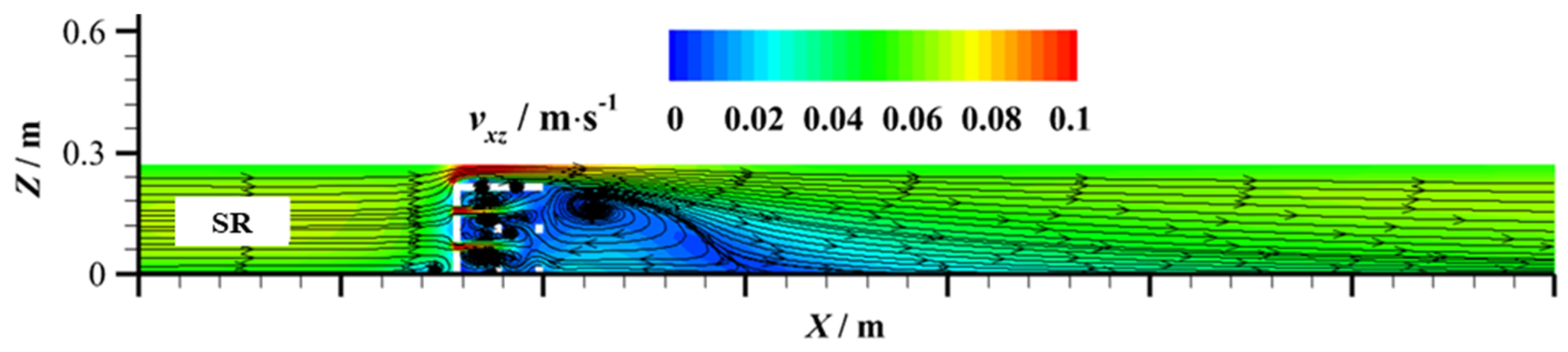
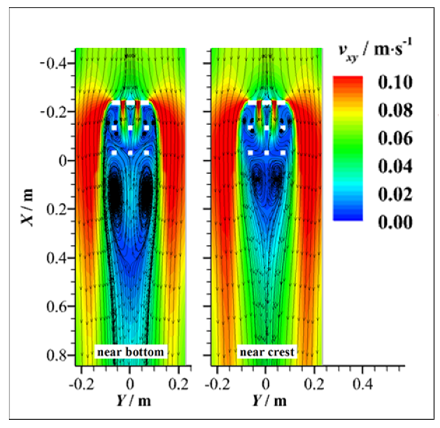
3.1. Flow Field

Numerical simulations are post-processed to obtain the time-averaged flow fields of the SR with the addition of streamlines under a constant inflow and submergence, and under different inflows and submergences, respectively.

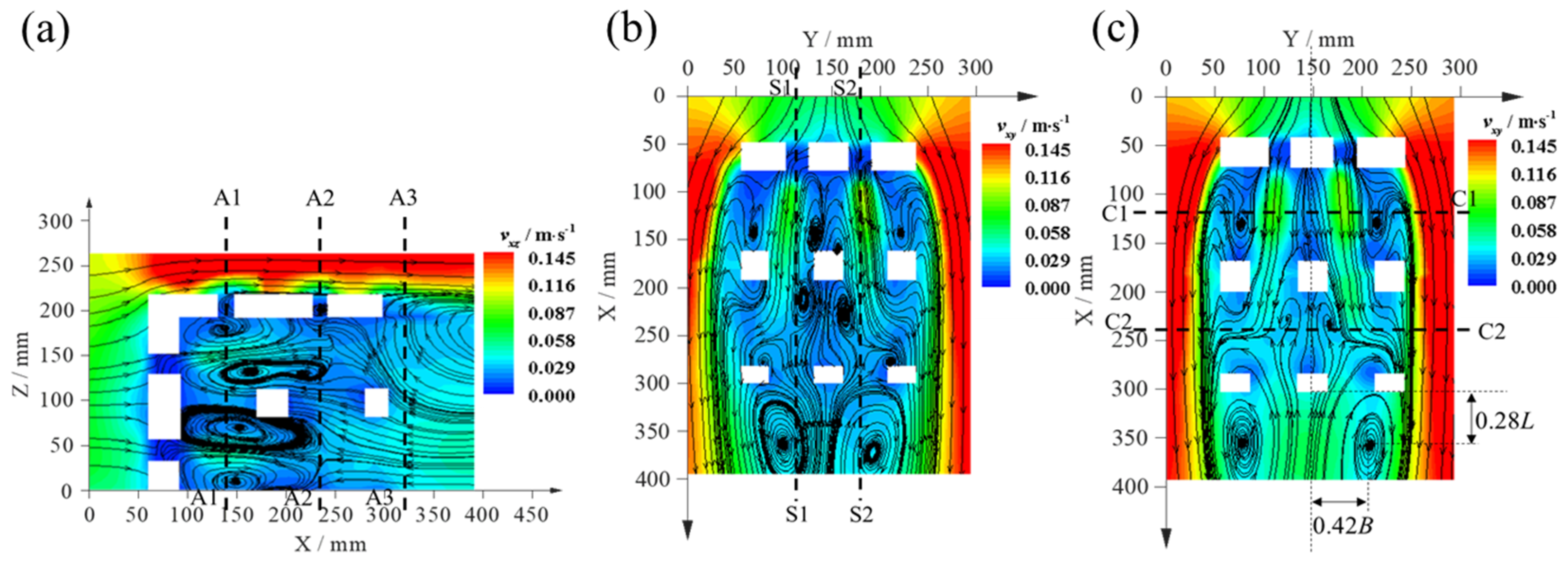
3.1.1. Vertical and Transversal Flow Fields under a Constant Inflow and Submergence

Figure 7 shows the vertical flow field of the SR (when R/h is 0.17, inflow velocity is 0.09 m/s), where the vector lines represent streamlines and the color contour map represents velocity magnitude. As the main flow passes through the SR, the streamline is gradually lifted due to the blocking effect of the SR, resulting in upwelling above the SR. Although most of the mainstream flow is blocked by the stoss face, part of flow enters into the SR compartment through the stoss face openings. The flow velocity through the opening holes is reduced by the wall resistance, and there are two quasi-symmetrical vortices in the fore half of the SR compartment because of the inflow, which has a jet-like effect. Meanwhile, the smallest scale vortices in the flow field are formed in the opening holes of the crest. As the upwelling converges to the mainstream, prevailing current flows over the SR towards the downstream. The flow creates a larger wake region behind the SR, which contains a large-scale clockwise vortex. The wake current flows from the leeside of the SR, which dominates the flow pattern within the SR compartment.

Figure 8 shows the transversal flow fields of the SR (when R/h is 0.17, inflow velocity is 0.09 m/s) at the near bottom (Z = 0.068 m) and near crest layers (Z = 0.156 m), incorporating the flow velocity contours and streamline. The structure of the flow field formed by the SR is similar at two transversal layers. When the water flow passes through the SR, the main flow section is narrowed, and a high-velocity zone (vxy ≥ 0.10 m·s⁻¹) is formed on both lateral sides of the SR, causing the water to flow downstream, and a pair of transversal vortices are formed in the back wake. Inside the compartment of the SR, two quasi-symmetrical high-velocity zones are formed behind the openings on the stoss face of the SR. This indicates that although the velocity in the opening holes is reduced by the SR crest reef friction resistance, the inflow through the openings induces a jet-like effect. As a whole, the transversal flow fields are occupied by several different sized vortices and form two sets of Continuous Vortex Streets around the square column inside the SR. In addition, the vortex distribution shows a certain symmetry in the lateral direction due to the symmetry of the SR structure.

The size of the transversal back vortex formed on the near bottom layer is much larger than that on the near crest layer. Since the flow field on the bottom layer is subject to greater bottom friction, the vortices are pulled into a longer shape by turbulent viscous forces. More vortices are formed on the near crest layer than that on the near bottom layer because the near crest flow is influenced by the SR crest with more energy dissipation. Similarly, in the transversal flow field, more vortices are generated in the fore half of the SR, consistent with those in the vertical flow field.

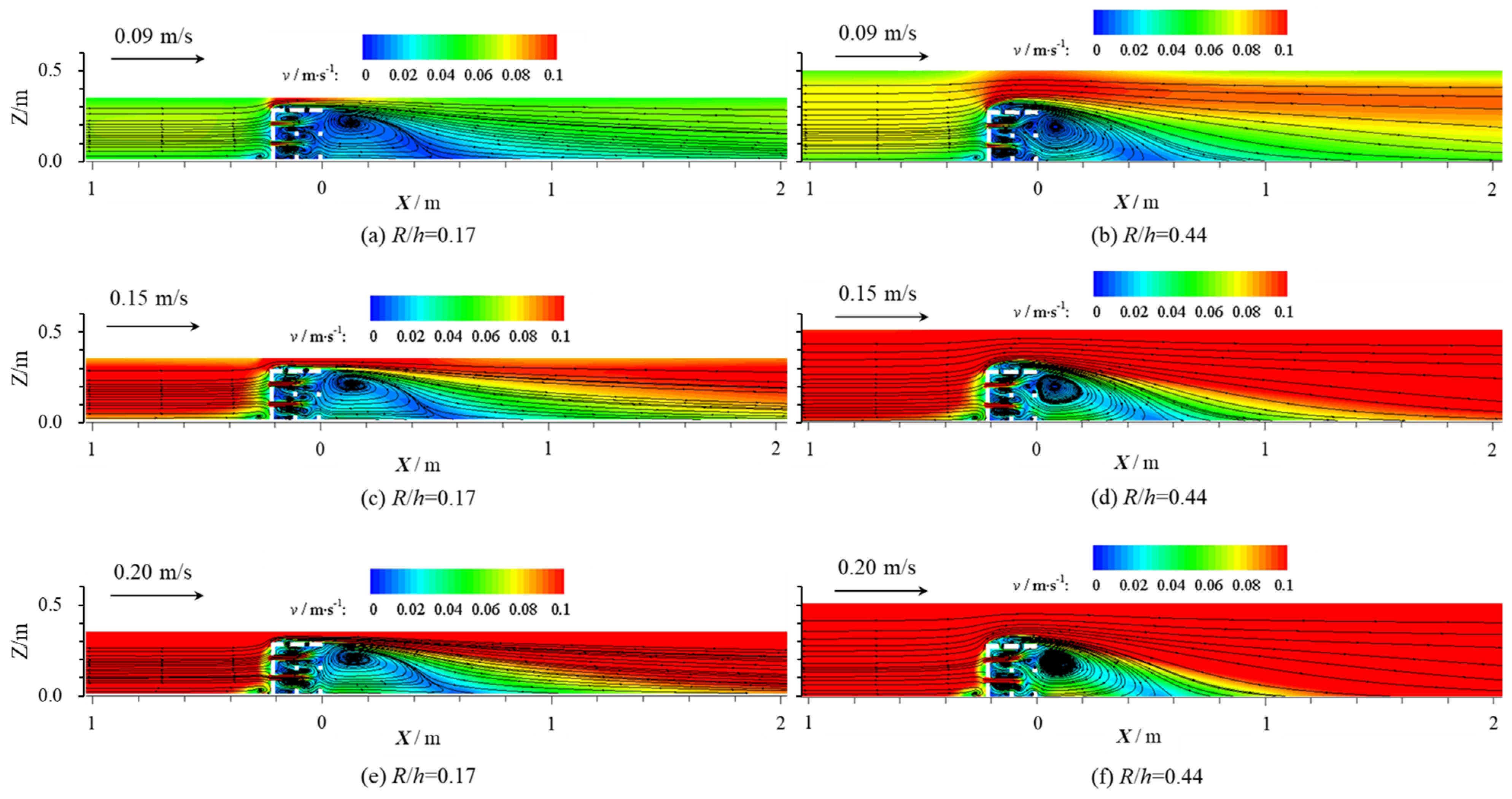
3.1.2. Flow Fields under Different Inflows and Submergences

The vertical flow field pattern reflects the primary turbulent structure characteristics and distribution range of the SR. Additionally, the distribution features of the transversal flow fields at different depths depend on the formation of vertical turbulent structure. Therefore, this section concentrates on analyzing and discussing the changes in the vertical flow field under different inflow and submergence conditions.

Flow fields induced by the SR under different constant inflows and submergences are shown in Figure 9. As shown in the figure, a small angular vortex forms in front of the SR under different conditions. This is because the increased friction near the bottom leads to a stagnant zone at the junction between the stoss face and the flume bottom when the main flow encounters the stoss face. Under the effect of different inflow velocities and submergences, the different shapes, sizes, and strengths of flow structure form within the SR. For the same R/h, the high-velocity jet-like flow region of the inner SR expands with the increasing velocity, and the velocity in the near bottom in the back wake is strengthened. Under the same velocity, the vortex region of the inner behind SR is bigger when R/h = 0.44 than when R/h = 0.17; the low velocity area above the crest expands and the velocity near bottom in the back wake is also increased.

3.2. Vorticity Pattern

Vortices are evident in fluid motion and have an important influence on the flow field, which is a key factor in triggering the vibration of the SR as well as energy dissipation. As mentioned before, it can be seen that vortex structures of various scales are generated in the vicinity of the SR, and the internal vortex structure is the main medium connecting the fluid motion inside and outside the structure. The ecological effect of the SR can be enhanced by the vortex. Therefore, it is significant to analyze the vortex field formed inside the SR compartment. The vorticity, defined as the spin of the flow field, is used to characterize the vortex motion in the flow field, which is considered as a collection of composite moving fluid vectors. The numerical data of the flow fields were used to generate the vorticity contours in the vertical and transversal planes. Ω_y and Ω_z are used for the vorticity along the transversal and vertical profiles, respectively, which are defined as:

$${\Omega }_y=\frac{\partial v_z}{\partial x}-\frac{\partial v_x}{\partial z}$$

(1)

$${\Omega }_z=\frac{\partial v_y}{\partial x}-\frac{\partial v_x}{\partial y}$$

(2)

where $v_x$ is the longitudinal velocity component; $v_y$ is the transverse velocity component; $v_z$ is the vertical velocity component; and Ω_y and Ω_z are the rotational strengths of the recirculating flow along the transverse and vertical directions, respectively.

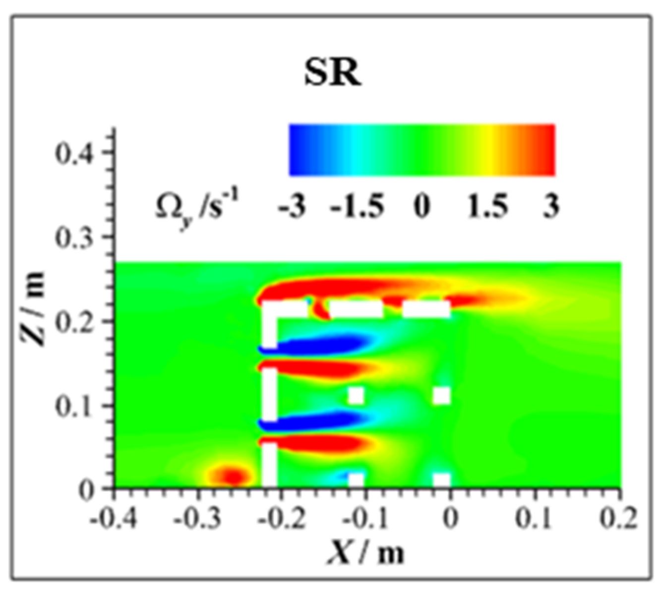
3.2.1. Vertical and Transversal Vorticity Patterns under a Constant Inflow and Submergence

Figure 10 shows the calculated results of the vertical vorticity pattern in the vicinity of the SR (when R/h is 0.17, inflow velocity is 0.09 m/s). These results show that high-vorticity dipoles are produced inside and behind the openings of the stoss face. When the flow passes through the holes, vortices are formed due to the change in velocity and the bending of the flow lines. For this reason, two pairs of strip-like vorticity dipoles containing positive and negative vortices are formed correspondingly behind two stoss face openings. The presence of vortices allows the rotation of the fluid at the microscopic scale to create vorticity. Above the SR crest, a positive vorticity region with higher magnitude is formed and extended to the rear of the SR. This indicates that the increasing flow velocity and bending of the flow lines may cause a greater rotational flow effect as it passes through the crest holes, resulting in the formation of larger vortices and greater vorticity.

Figure 11 shows the transversal vorticity distribution in the vicinity of the SR (when R/h is 0.17, inflow velocity is 0.09 m/s) on the near bottom and near crest layers. The vorticity distribution is similar in both planes. High-vorticity regions are generated on both lateral sides of the SR as well as within the SR. The high-vorticity regions on both sides extend downstream, while the shear stress layer is enlarged due to the fluid viscosity, resulting in a larger high-vorticity region. The internal high vorticity is concentrated in the front half of the SR, and there are two pairs of dipole-type high-vorticity clouds with opposite directions behind two openings of the SR stoss face. In addition, the vorticity of the near bottom layer is slightly weaker than that of the near crest layer because of the stronger influence of the SR crest.

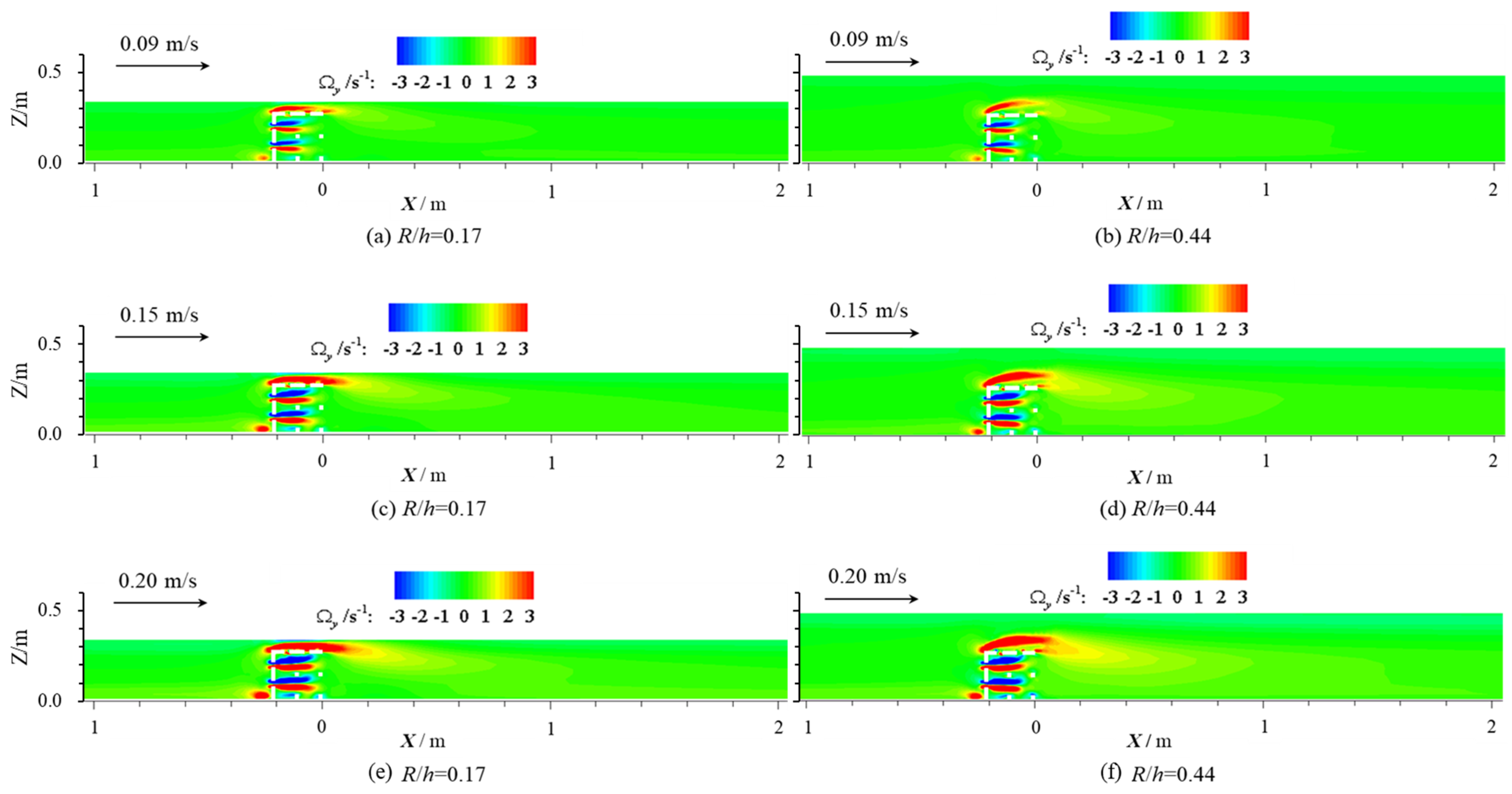
3.2.2. Vorticity Patterns under Different Constant Inflows and Submergences

Figure 12 shows the vorticity distribution in the vicinity of the SR under different constant inflows and submergences. In general, the dipole structures with high vorticity form inside the SR and their location in each case are basically the same, while the range and magnitude of the high-vorticity region differ significantly. With respect to the same R/h, the range of the high-vorticity zone spreads and the contained vorticity value gradually increases with the increase in inflow velocity, indicating that the vortex structure at the same location is strengthened by the increase inflows. With respect to the same inflow velocity, the range of the high-vorticity zone expands vertically and constricts transversally with the increase in R/h.

3.3. Turbulent Intensity

Turbulence, as a complex flow regime prevalent in nature, has a significant impact on fish migration. As an important reference indicator, turbulent intensity is usually used to characterize turbulence and assess coastal fish habitat suitability. Therefore, the distribution of turbulent intensity in the vicinity of the SR attracts major concerns. Turbulent intensity is defined as the ratio of the standard deviation of the fluctuating velocity to the mean velocity, representing the intensity of the flow fluctuations [44]. In this section, $I_{xy}$ and $I_{xz}$ represent the total turbulent intensity in the transversal and vertical profiles, respectively. The calculation details of turbulent intensity can be observed in [33].

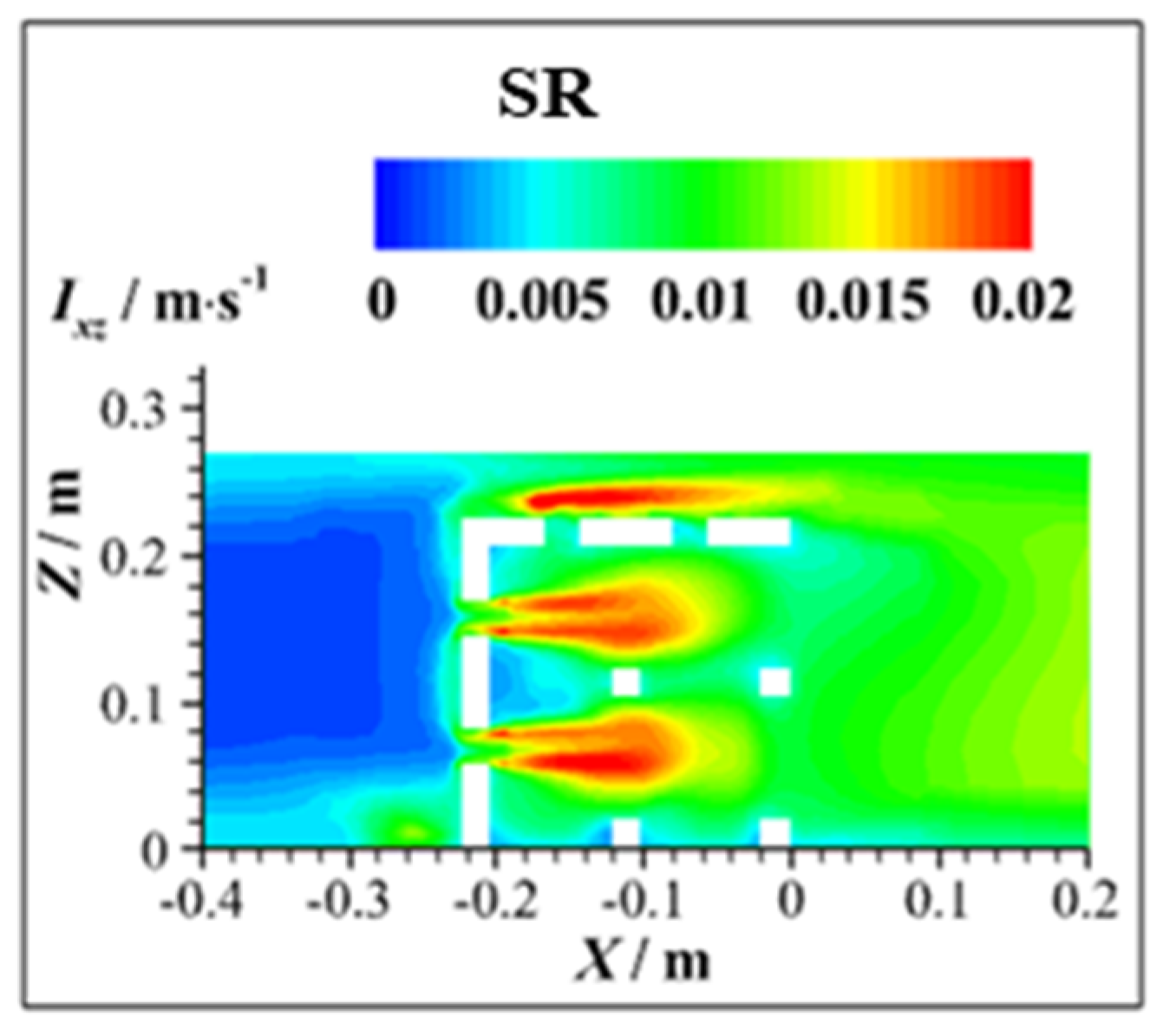
3.3.1. Vertical and Transversal Turbulent Intensity Distribution under a Constant Inflow and Submergence

Vertical turbulent intensity inside the compartment of the SR (when R/h is 0.17, inflow velocity is 0.09 m/s) is shown in Figure 13. The turbulent intensity in front of the SR is relatively small due to the blocking effect of the SR structure. However, when the flow contacts the flume bottom and the free surface, the flow velocity gradient varies considerably due to the effect of the friction, and the turbulent intensity increases accordingly. As a result, a significant gradient in the flow perpendicular to the wall may lead to an increase in the turbulent intensity. In addition, the turbulent intensity above the crest is also strong as the flow rises over the SR. Since the flow velocity changes sharply over the crest’s perforated holes, stronger disturbance and higher turbulent intensity are produced.

Figure 14 shows the transversal turbulent intensity distributed on the near bottom and near crest layers (when R/h is 0.17, inflow velocity is 0.09 m/s). It can be seen that turbulent intensity is generated on both lateral sides, the interior, and the rear of the SR. Strong turbulent regions ($I_{xy}>0.016\mathrm{m}/\mathrm{s}$) are formed both inside and behind the structure, and the turbulent intensity on the near bottom layer is greater than that on the near crest layer. The reason for this is the drag effect on the near bottom layer is prominent, causing the lower velocity and more turbulent intensity than that on the near crest layer.

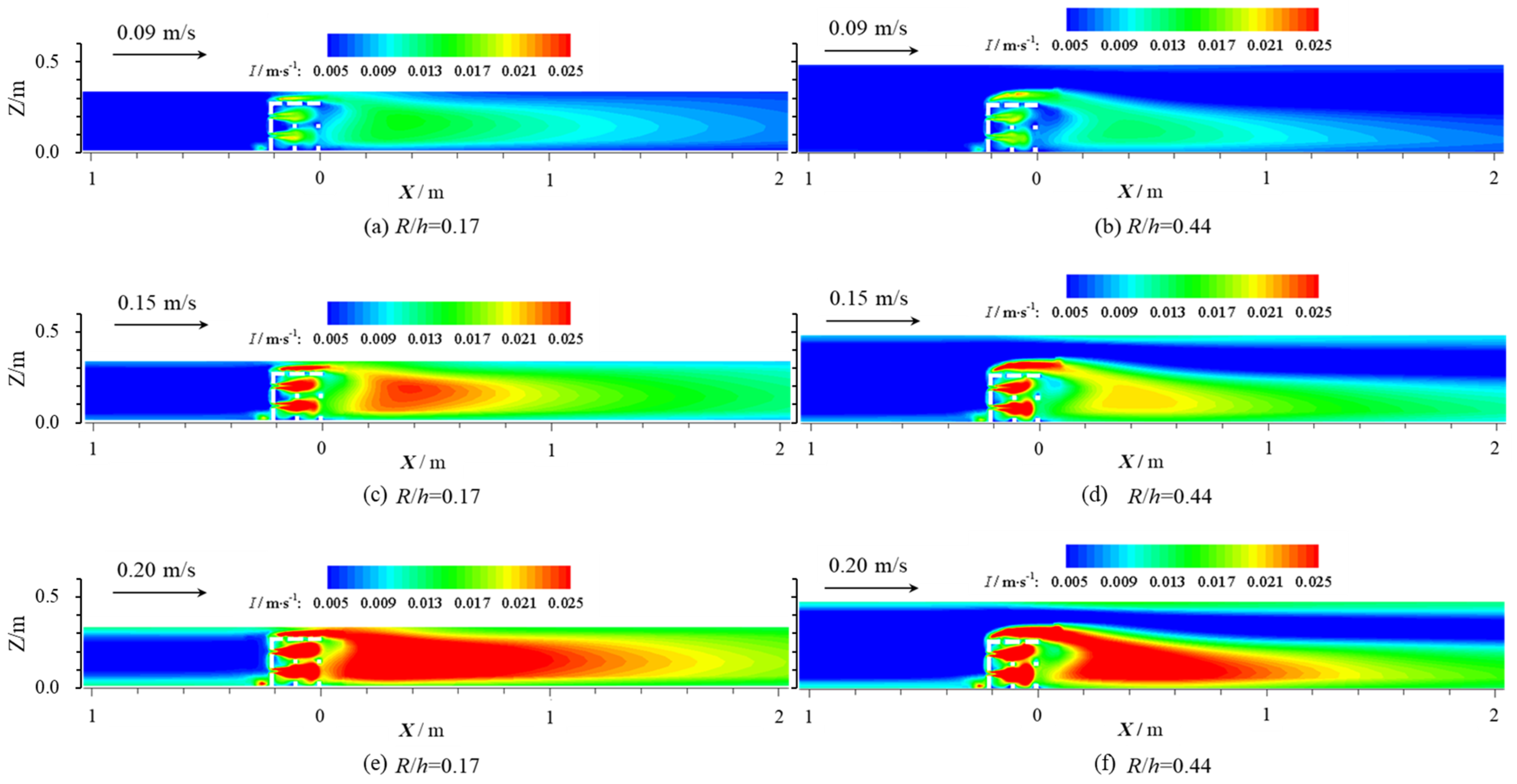
3.3.2. Turbulent Intensity Distribution under Different Constant Inflows and Submergences

The vertical turbulent intensity distribution in the vicinity of the SR under different inflows and submergences is given in Figure 15. The turbulent intensity is calculated as the root mean square of the fluctuated flow velocity, which represents the fluctuation of the flow velocity. In relation to the same R/h, the turbulent intensity gradually increases with the raising inflow velocity, both inside and behind the SR. Similarly, in relation to the same inflow velocity, the turbulent intensity inside and behind the SR decreases with the increasing R/h value. This phenomenon also explains the reason why the vortex dipole inside the SR is larger under smaller submergence, as shown in Figure 12.

4. Discussion

The back wake area behind the leeside of the SR is often a low-speed, slow-flowing area containing a large number of wakes that provide fish with breeding and roosting sites [45]. And the vorticity pattern strength generated within the SR is strongly correlated with fish abundance [37]. In particular, the length of the back wake and the high-vorticity dipoles are chosen to quantify the influence of inflow and submergence, which can provide a reference for SR deployments.

4.1. The Impact of Inflow and Submergence on the Length of the Back Wake

The back wake is the largest turbulent structure in the flow field, which has a good shielding effect. In order to quantitatively analyze the change characteristics of this back wake under different inflows and submergences, the lengths of the back wake are extracted and calculated under different conditions. The length of the back wake was divided by the length of the SR (lr) to obtain the dimensionless relative back wake lengths for further analysis, and the calculated results are listed in

Table 2. The relative length of back wake of the SR under different inflows and submergences.

Inflow Velocity (m/s)	R/h = 0.17	R/h = 0.44
0.09	2.11	2.24
0.15	2.24	2.39
0.20	2.31	2.51

. As shown in the table, in terms of the same R/h, the back wake length increases with the increase in inflow velocity. In terms of the same inflow velocity, the increase in R/h results in an extension of the back wake length. It indicates that the inflow velocity and R/h are positively and linearly correlated with the back wake length.

4.2. The Impact of Inflow and Submergence on the High-Vorticity Dipoles

The variation rule of the high-vorticity dipoles inside the SR under different inflows and submergences are quantitatively elucidated by extracting the high-vorticity area with |Ω_y| > 1.5 s⁻¹ and the corresponding mean vorticity values, the results are listed in

Table 3. The area and average value of high vorticity (|Ω_y| > 1.5 s⁻¹) inside the SR under different inflows and submergences.

Inflow Velocity (m/s)	R/h = 0.17				R/h = 0.44
	Area (×10−3 m2)		Mean Vorticity (s−1)		Area (×10−3 m2)		Mean Vorticity (s−1)
	Ωy > 1.5 s−1	Ωy < −1.5 s−1	Ωy > 1.5 s−1	Ωy < −1.5 s−1	Ωy > 1.5 s−1	Ωy < −1.5 s−1	Ωy > 1.5 s−1	Ωy < −1.5 s−1
0.09	4.074	4.085	3.701	−3.801	3.983	3.973	3.688	−3.771
0.15	7.202	6.704	4.905	−5.083	6.495	6.246	5.198	−5.205
0.20	9.021	8.266	5.923	−6.169	7.832	7.368	6.397	−6.411

. For the same R/h, the area and intensity of the high-vorticity region gradually increase with the raising inflow velocity. For the same inflow velocity, the area of the dipole inside the SR reduces with the increase in R/h, while the mean vorticity value decreases at an inflow velocity of 0.09 m/s and increases at a higher inflow velocity. It can be interpreted that the free water surface is closer to the SR crest when R/h is 0.17, leading to greater fluid turbulence and instability inside, resulting in the formation of vorticity dipoles with larger areas. Additionally, when the inflow velocity is lower, the free water surface’s influence is stronger.

5. Conclusions

This study investigated turbulent features in the vicinity of the perforated SR under different constant inflow and submergence conditions by well-validated numerical modelling, focusing on the three-dimensional characteristics of the back wake length and inner flow patterns. The main conclusions are as follows:

(a)

As the main flow passes through the SR, the upwelling is produced in front of the SR and a large-scale wake region is formed behind the SR, which contains a clockwise vortex. The vortex structure formed inside the SR is induced by the interaction between wake currents from the lee side and the jet-like flow from the stoss face openings.

(b)

In terms of the same submergence, as the inflow velocity increases, the relative back wake length increases gradually, as well as the area and mean values of the high-vorticity region inside the SR. The turbulent intensity distributed inside and behind the SR is enhanced with a higher inflow velocity.

(c)

In terms of the same inflow velocity, as the submergence increases, the relative back wake length increases, while the high-vorticity region above the SR crest expands along the vertical direction and constricts along the longitudinal direction. The area of high-vorticity dipoles within the SR decreases as submergence increases, while the mean vorticity value decreases at an inflow velocity of 0.09 m/s and increases at a higher inflow velocity. Moreover, the turbulent intensity in the vicinity of the SR gradually attenuates.

This study can give guidance on the placement of SRs in coastal engineering, while in practical engineering the SR will be subject to flood tide, ebb tide, and ocean waves. In our further study, the mechanisms of SRs on wave nonlinearity, energy exchange, and turbulence distribution under wave-current combined actions will be discussed.

References

- Jiang, Z.; Liang, Z.; Tang, Y.; Huang, L.; Yu, D.; Jiang, M. Numerical Simulation and Experimental Study of the Hydrodynamics of a Modeled Reef Located within a Current. Chin. J. Oceanol. Limnol. 2010, 28, 267–273. [Google Scholar] [CrossRef]
- Kallianiotis, A.A.; Batjakas, I.E. Temporal and Environmental Dynamics of Fish Stocks in the Marine Protected Area of the Artificial Reef of Kitros, Pieria (Northern Greece, Mediterranean Sea). J. Mar. Sci. Eng. 2023, 11, 1773. [Google Scholar] [CrossRef]
- Oteiza, P.; Odstrcil, I.; Lauder, G.; Portugues, R.; Engert, F. A Novel Mechanism for Mechanosensory-Based Rheotaxis in Larval Zebrafish. Nature 2017, 547, 445–448. [Google Scholar] [CrossRef]
- Ng, K.; Phillips, M.R.; Calado, H.; Borges, P.; Veloso-Gomes, F. Seeking Harmony in Coastal Development for Small Islands: Exploring Multifunctional Artificial Reefs for São Miguel Island, the Azores. Appl. Geogr. 2013, 44, 99–111. [Google Scholar] [CrossRef]
- Relini, G.; Relini, M.; Palandri, G.; Merello, S.; Beccornia, E. History, Ecology and Trends for Artificial Reefs of the Ligurian Sea, Italy. Hydrobiologia 2007, 580, 193–217. [Google Scholar] [CrossRef]
- Bohnsack, J.A.; Johnson, D.L.; Ambrose, R.F. 3—Ecology of Artificial Reef Habitats and Fishes. In Artificial Habitats for Marine and Freshwater Fisheries; Seaman, W., Sprague, L.M., Eds.; Academic Press: San Diego, CA, USA, 1991; pp. 61–107. ISBN 978-0-08-057117-1. [Google Scholar]
- Hirose, N.; Watanuki, A.; Saito, M. New Type Units for Artificial Reef Development of Eco-Friendly Artificial Reefs and the Effectiveness Thereof. In 30th PIANC-AIPCN Congress 2002; Institution of Engineers: Sydney, Australia, 2002. [Google Scholar]
- Armono, H. Wave Transmission on Submerged Breakwaters Made of Hollow Hemispherical Shape Artificial Reefs. In Proceedings of the Canadian Coastal Conference, Kingston, ON, Canada, 15–17 October 2003; Volume 2003. [Google Scholar]
- Buccino, M.; Del Vita, I.; Calabrese, M. Predicting Wave Transmission Past Reef BallTM Submerged Breakwaters. J. Coast. Res. 2013, 65, 171–176. [Google Scholar] [CrossRef]
- Srisuwan, C.; Rattanamanee, P. Modeling of Seadome as Artificial Reefs for Coastal Wave Attenuation. Ocean Eng. 2015, 103, 198–210. [Google Scholar] [CrossRef]
- Van Gent, M.R.A.; Buis, L.; Van Den Bos, J.P.; Wüthrich, D. Wave Transmission at Submerged Coastal Structures and Artificial Reefs. Coast. Eng. 2023, 184, 104344. [Google Scholar] [CrossRef]
- Metallinos, A.S.; Repousis, E.G.; Memos, C.D. Wave Propagation over a Submerged Porous Breakwater with Steep Slopes. Ocean Eng. 2016, 111, 424–438. [Google Scholar] [CrossRef]
- Panizzo, A.; Briganti, R. Analysis of Wave Transmission behind Low-Crested Breakwaters Using Neural Networks. Coast. Eng. 2007, 54, 643–656. [Google Scholar] [CrossRef]
- Tsai, C.-C.; Chang, Y.-H.; Hsu, T.-W. Step Approximation on Oblique Water Wave Scattering and Breaking by Variable Porous Breakwaters over Uneven Bottoms. Ocean Eng. 2022, 253, 111325. [Google Scholar] [CrossRef]
- Zheng, S.; Meylan, M.; Zhang, X.; Iglesias, G.; Greaves, D. Performance of a Plate-wave Energy Converter Integrated in a Floating Breakwater. IET Renew. Power Gener. 2021, 15, 3206–3219. [Google Scholar] [CrossRef]
- Khan, M.B.M.; Gayathri, R.; Behera, H. Wave Attenuation Properties of Rubble Mound Breakwater in Tandem with a Floating Dock against Oblique Regular Waves. Waves Random Complex Media 2021, 1–19. [Google Scholar] [CrossRef]
- Naik, N.; Behera, H. Role of Dual Breakwaters and Trenches on Efficiency of an Oscillating Water Column. Phys. Fluids 2023, 35, 047115. [Google Scholar] [CrossRef]
- Fang, L.; Chen, P.; Chen, G.; Tang, Y.; Yuan, H.; Feng, X. Preliminary Evaluation on Resources Enhancement of Artificial Reef in the East Corner of Zhelang Shanwei. Asian Agric. Res. 2013, 5, 111–115. [Google Scholar] [CrossRef]
- Liu, T.-L.; Su, D.-T. Numerical Analysis of the Influence of Reef Arrangements on Artificial Reef Flow Fields. Ocean Eng. 2013, 74, 81–89. [Google Scholar] [CrossRef]
- Jang, S.-C.; Jeong, J.-Y.; Lee, S.-W.; Kim, D. Identifying Hydraulic Characteristics Related to Fishery Activities Using Numerical Analysis and an Automatic Identification System of a Fishing Vessel. J. Mar. Sci. Eng. 2022, 10, 1619. [Google Scholar] [CrossRef]
- Lin, J.; Zhang, S. Research Advances on Physical Stability and Ecological Effects of Artificial Reef. Marine Fish./Haiyang Yuye 2006, 28, 257–262. [Google Scholar]
- Tang, Y.L.; Long, X.Y.; Wang, X.X.; Jiang, Z.Y.; Cheng, H.; Zhang, T.Z. Comparative analysis on flow field effect of general artifi-cial reefs in China. Trans. Chin. Soc. Agric. Eng. 2017, 33, 97–103. [Google Scholar] [CrossRef]
- Jiang, Z.Y. Artificial Reef Hydrodynamics and Numerical Simulation Study. Ph.D. Thesis, Ocean University of China, Qingdao, China, 2009. [Google Scholar]
- Maslov, D.; Pereira, E.; Duarte, D.; Miranda, T.; Ferreira, V.; Tieppo, M.; Cruz, F.; Johnson, J. Numerical Analysis of the Flow Field and Cross Section Design Implications in a Multifunctional Artificial Reef. Ocean Eng. 2023, 272, 113817. [Google Scholar] [CrossRef]
- Kim, D.; Woo, J.; Yoon, H.S.; Na, W.B. Efficiency, tranquillity and stability indices to evaluate performance in the artificial reef wake region. China Ocean Eng. 2016, 122, 253–261. [Google Scholar] [CrossRef]
- Paxton, A.B.; Peterson, C.H.; Taylor, J.C.; Adler, A.M.; Pickering, E.A.; Silliman, B.R. Artificial reefs facilitate tropical fish at their range edge. Commun. Biol. 2019, 2, 168. [Google Scholar] [CrossRef]
- Fabi, G.; Grati, F. Adriatic Sea: The role of artificial reefs in the marine spatial planning. In Proceedings of the RECIF Conference on Artificial Reefs: From Materials to Ecosystem, Caen, France, 27–29 January 2015. [Google Scholar]
- Gates, A.R.; Horton, T.; Serpell-Stevens, A.; Chandler, C.; Grange, L.J.; Robert, K.; Bevan, A.; Jones, D.O.B. Ecological role of an offshore industry artificial structure. Front. Mar. Sci. 2019, 6, 675. [Google Scholar] [CrossRef]
- Spring, D.L.; Williams, G.J. Influence of Upwelling on Coral Reef Benthic Communities: A Systematic Review and Meta-Analysis. Proc. R. Soc. B Biol. Sci. 2023, 290, 20230023. [Google Scholar] [CrossRef]
- Stocking, J.; Rippe, J.; Reidenbach, M. Structure and Dynamics of Turbulent Boundary Layer Flow over Healthy and Algae-Covered Corals. Coral Reefs 2016, 35, 1047–1059. [Google Scholar] [CrossRef]
- Stocking, J.; Laforsch, C.; Sigl, R.; Reidenbach, M. The Role of Turbulent Hydrodynamics and Surface Morphology on Heat and Mass Transfer in Corals. J. R. Soc. Interface 2018, 15, 20180448. [Google Scholar] [CrossRef] [PubMed]
- Reidenbach, M.A.; Stocking, J.B.; Szczyrba, L.; Wendelken, C. Hydrodynamic Interactions with Coral Topography and Its Impact on Larval Settlement. Coral Reefs 2021, 40, 505–519. [Google Scholar] [CrossRef]
- Zheng, Y.; Kuang, C.; Zhang, J.; Gu, J.; Chen, K.; Liu, X. Current and turbulent characteristics of perforated box-type artificial reefs in a constant water depth. Ocean Eng. 2022, 244, 110359. [Google Scholar] [CrossRef]
- Silva, A.T.; Katopodis, C.; Santos, J.M.; Ferreira, M.T.; Pinheiro, A.N. Cyprinid Swimming Behaviour in Response to Turbulent Flow. Ecol. Eng. 2012, 44, 314–328. [Google Scholar] [CrossRef]
- Silva, A.T.; Santos, J.M.; Ferreira, M.T.; Pinheiro, A.N.; Katopodis, C. Effects of Water Velocity and Turbulence on the Behaviour of Iberian Barbel (Luciobarbus Bocagei, Steindachner 1864) in an Experimental Pool-Type Fishway. River Res. Appl. 2011, 27, 360–373. [Google Scholar] [CrossRef]
- Goettel, M.T.; Atkinson, J.F.; Bennett, S.J. Behavior of Western Blacknose Dace in a Turbulence Modified Flow Field. Ecol. Eng. 2015, 74, 230–240. [Google Scholar] [CrossRef]
- Fischer, J.L.; Filip, G.P.; Alford, L.K.; Roseman, E.F.; Vaccaro, L. Supporting Aquatic Habitat Remediation in the Detroit River through Numerical Simulation. Geomorphology 2020, 353, 107001. [Google Scholar] [CrossRef]
- Hashempour, M.; Kolahdoozan, M. Three-Dimensional Modeling of Dilute Sediment Concentration around the Synthetic Sponge Inspired by the Tubular Sponge Mechanism. Ocean Eng. 2023, 271, 113799. [Google Scholar] [CrossRef]
- Hashempour, M.; Kolahdoozan, M. Inspiration of Marine Sponges to Design a Structure for Managing the Coastal Hydrodynamics and Protection: Numerical Study. Front. Mar. Sci. 2023, 10, 1091540. [Google Scholar] [CrossRef]
- Van Heijst, G.J.F.; Flor, J.B. Dipole formation and collisions in a stratified fluid. Nature 1989, 340, 212–215. [Google Scholar] [CrossRef]
- Pope, S.B. Turbulent Flows; Cambridge University Press: Cambridge, UK, 2000. [Google Scholar]
- Nst, O.A.; Brve, E. Flow separation, dipole formation and water exchange through tidal strait. Ocean. Sci. 2021, 17, 1403–1420. [Google Scholar] [CrossRef]
- Afanasyev, Y. Formation of vortex dipoles. Phys. Fluids 2006, 18, 159. [Google Scholar] [CrossRef]
- ANSYS. Ansys-Fluent, Release 17.0; ANSYS Inc.: Canonsburg, PA, USA, 2017. [Google Scholar]
- Li, X.; Luan, S.; Chen, Y.; Zhang, R. The 3D vortex structure of cube artificial reef’s wake vortex. J. Dalian Ocean. Univ. 2012, 27, 572–577. [Google Scholar] [CrossRef]