Utilizing Machine Learning Tools for Calm Water Resistance Prediction and Design Optimization of a Fast Catamaran Ferry

Abstract

The article aims to design a calm water resistance predictor based on Machine Learning (ML) Tools and develop a systematic series for battery-driven catamaran hullforms. Additionally, employing a machine learning predictor for design optimization through the utilization of a Genetic Algorithm (GA) in an expedited manner. Regression Trees (RTs), Support Vector Machines (SVMs), and Artificial Neural Network (ANN) regression models are applied for dataset training. A hullform optimization was implemented for various catamarans, including dimensional and hull coefficient parameters based on resistance, structural weight reduction, and battery performance improvement. Design distribution based on Lackenby transformation fulfills all of the design space, and sequentially, a novel self-blending method reconstructs new hullforms based on two parents blending. Finally, a machine learning approach was conducted on the generated data of the case study. This study shows that the ANN algorithm correlates well with the measured resistance. Accordingly, by choosing any new design based on owner requirements, GA optimization obtained the final optimum design by using an ML fast resistance calculator. The optimization process was conducted on a 40 m passenger catamaran case study that achieved a 9.5% cost function improvement. Results show that incorporating the ML tool into the GA optimization process accelerates the ship design process.

1. Introduction

The EU-funded project “TrAM-Transport: Advanced and Modular” develops battery-driven zero-emission fast passenger vessels for coastal areas and inland waterways. Modular design and manufacturing methods are the focus of this project, with the objectives of minimizing environmental impact and life cycle cost [1,2]. The development of a systematic series of zero-emission catamaran hullforms for different displacement tonnage and ship types can significantly help this process. Enormous catamaran hullforms will be generated during the systematic series development, and resistance calculation takes time for each design. An accurate and fast resistance predictor leads to a convenient tool for a class of hullforms. Therefore, a new model for such diversity with appropriate generalization to new predictions is desired in this field, leading to data mining approaches [3]. ML can be combined with optimization algorithms to efficiently explore the design space and identify optimal or near-optimal solutions. Genetic algorithms, particle swarm optimization, and other optimization techniques can benefit from ML models to guide the search process and converge to better solutions faster. By leveraging these techniques, naval architects and ship designers can streamline the hullform optimization process, reduce the need for time-consuming simulations, and ultimately arrive at more efficient and cost-effective ship designs [4].

2. Background

Resistance calculations in past decades have been implemented by model tests or sea trial measurements. Classic regression models are limited to conventional vessels with specified general particulars. Traditional methods of resistance prediction involve extensive model testing, computational fluid dynamics (CFD) simulations, and empirical correlations. However, the complexity of catamaran hullforms, coupled with the desire for enhanced design efficiency, necessitates a paradigm shift in the approach to resistance prediction [5]. Enter machine learning—a transformative tool capable of extracting intricate patterns from vast datasets, promising to revolutionize the maritime design landscape [6]. Accordingly, the current study embarks on a comprehensive exploration of the systematic series development and calm water resistance prediction for fast catamaran ferries. We leverage the power of machine learning tools to augment traditional design methodologies, seeking to enhance accuracy, efficiency, and the overall efficacy of the design process. Additionally, a Genetic Algorithm optimization study will be implemented on a sample design by using a machine learning resistance predictor as a fast approach objective calculation method.

Ship resistance optimization plays an important role in hullform development. Assessing the ship resistance in the first stage of ship design allows the designer to analyze the influence of different hullforms and parameters. Accordingly, different methods of geometry optimization and design study have been developed during past decades. Papanikolaou et al. [7] implemented a global and local hullform optimization of the fast catamaran in two design study scenarios. In the first stage of optimization, 1000 hullforms were elaborated with a surrogate-based design study using a potential theory 3D panel code. After that, the two most promising designs were selected as the initial hullform for local modification, focusing on the stern region. However, a comprehensive design optimization might be proposed according to balance accuracy and time [8]. An all-inclusive hullform optimization in the field of ship design defines various hullforms with different geometrical parameters. Accordingly, the marine industry needs an optimization platform to minimize the required propulsion power according to various possibilities of hullform. Additionally, a systematic series is developed on generated geometries to establish a resistance predictor.

Li et al. [9], by using Single-Parameter Lagrangian Support Vector Regression (SPL-SVR), developed a metamodel on seakeeping data. A multidisciplinary design optimization in the concept design stage of ships has been proposed. Recently, Fahrnholz and Caprace [10] conducted a regression analysis on three sailboats’ systematic series. Based on machine learning techniques, a resistance predictor was designed on resistance data. Nazemian and Ghadimi [11], by using a D-optimal DoE study, investigated the resistance performance of a trimaran hull series. A resistance analysis and its improvement were encompassed to extract the optimum value of hull parameters and sidehull arrangement.

Machine learning techniques have commenced in the last decade in the field of ship design and hydrodynamics [12,13]. Resistance prediction has been developed and compared with traditional approaches by Radojic et al. [14,15]. An Artificial Neural Network regression method was designed for planing boats at different series types. Machine learning models can also be implemented on added resistance [16] and ice resistance [17]. Different aspects of ship design targets can be considered in dataset analysis. Liu and Papanikolaou [18] developed a semi-empirical formula, approximating the added resistance of ships in regular waves of arbitrary heading. The development of a catamaran class alongside the optimization process has been considered in the current study with automatic design generation.

The present paper is divided into three phases; systematic series development for a fast passenger and freight zero-emission catamaran, applying machine learning on generated data, and hullform optimization using a developed resistance predictor. Based on surveyed literature, it can be concluded that a hullform optimization process needs to be added to ship series. For each tonnage condition and ship type, a predictive machine learning model is developed to calculate calm water resistance. Moreover, the final design would be the best design with respect to the lowest resistance at multi-design speeds. A genetic algorithm optimization process connects to the resistance predictor to calculate design objectives of the optimization process. In the frame of the TrAM project, various optimized design options are prepared based on ship dimension and coefficient and hullform alteration. Accordingly, the design study starts with numerous ship types and tonnage and offers different possibilities of catamaran hullform as flexibility for the owner’s selection. Owners can choose their optimized design based on their requirements. On the other hand, by selecting design requirements like ship dimensions from the ship owner and an ML fast-approach resistance predictor, an optimized design can be obtained from a Genetic Algorithm in a fast approach.

3. Methodology

The present design study code capabilities, allowing any type of hullform to be modelled in case of different ship design targets, offer scope for the creation of a wide range of hullforms and provide an optional selection for owners. Combined with the built-in resistance, structure weight, and battery-driven system performance calculations, you have the tools to experiment with shapes and explore design parameters. Accordingly, an extensive fast catamaran series has been created, and a resistance predictor model has been developed on the generated dataset. The case study is a catamaran hull [1,2] as an initial design for database production. The database consists of three tonnages (${∆}_1=75$, ${∆}_2=80$, ${∆}_3=85$) tons. Two types of passenger and freight catamaran boats are defined as the initial hullform. The general arrangement of the under-studied catamarans is depicted in Figure 1.

Firstly, a Machine Learning dataset is generated using shift transformation and self-blending methods. After that, total resistance is calculated for all generated hullforms via the slender body method. The structural weight of each design is estimated by a regression formula and shell expansion of the hull surface. The propulsion system of the vessel works with electrically powered battery spares. Performance and battery weight are computed based on resistance and consequently, the break power of the catamaran [19,20].

The framework of the design study and machine learning is illustrated in Figure 2. For each tonnage, ship geometry is designed and distributed on the design space according to a multi-level combination of design variables. Performing parametric transformations and self-blending methods creates a series of hullforms with systematically varying parameters, which have been coded in the MATLAB program (R2022b) [21]. Parametric transformation by moving ship sections and self-blending by moving Control Points implement parametric transformations to create new hulls. Accordingly, the design dataset will be prepared for the machine learning process. Outputs of the design study are total resistance, structure weight, and battery weight calculated for each design.

Pre-processing progress is applied to obtained data to define different regression schemes. Herein, Regression Tree (RT), Support Vector Regression (SVR), and Artificial Neural Network (ANN) methods are used to predict other interesting designs and find a resistance predictive model. Then, a fast-approach resistance predictor will be applied in optimization process, in which the Genetic Algorithm (GA) method will be used, which is shown in the second stage of Figure 2.

The case study catamaran is the prototype hullform, which is designed and built in frame of the Horizon 2020 European Research project TrAM [22]. The main purpose of this effort is to replicate this hullform based on small modifications. The optimization process is conducted on six design variables and two constraints that are shown in

Table 1. Design parameters of the catamaran case study for design optimization.

Optimization Parameter	Symbol	Specifications
Design Variable	Lwl	Waterline length (m)
Design Variable	B	Demi hull Beam (m)
Design Variable	T	Draft (m)
Design Variable	DT	Demi hull transverse distance (m)
Free Variable	Cb	Block coefficient
Design Variable	Cm	Max section area coefficient
Design Variable	LCB (% of Lwl)	Longitudinal Center of Buoyancy
Constraint	∇	Displacement (ton)
Constraint	(DT × 2) + B	Total Beam (m)

. The output of the optimization process is resistance at 12 knots and resistance at 22 knots, which is represented by a weighting cost function:

$$\begin{gathered} Cost function=\left(\left(\frac{{Rt}_{LowFn}}{{Rt}_{LowFn0}}\right)\times {Wt}_{LowFn}+\left(\frac{{Rt}_{HighFn}}{{Rt}_{HighFn0}}\right)\times {Wt}_{HighFn}+(Weight/ \\ Weight0)\times {Wt}_{Weight}\right)\times \left(\frac{Disp0}{Disp\_get}\times \frac{1}{1000}\right), \end{gathered}$$

(1)

The resistance at a low Froude number signifies as Rt_LowFn, indicating resistance at 12 knots. Rt_HighFn corresponds to the resistance at a high Froude number, contributing to resistance at 22 knots. Weight pertains to the lightweight design of the ship, nondimensionalized against the initial design weight. Disp0 and Disp_get respectively represent the displacements of the initial hull and the displacement of the new hull, calculated from hydrostatic data. Alterations in the shape and geometry of the ship hull are achieved by imposing a constraint that maintains the difference in displacement under 1%. If displacement is the sole constraint, the length, breadth, and draft are automatically adjusted to accommodate the hull geometry redistributed volume. Consequently, the displacement constraint is defined as follows:

$$\left|\frac{{∆}_{new}-{∆}_{org}}{{∆}_{org}}\right|\le 0.01,$$

(2)

Another constraint of the present study is the total beam of the catamaran to satisfy port requirements, therefore:

$$2\times Demi hull offset+demi hull beam\le 9,$$

(3)

Demi hull offset is the distance between centerline of each demi hull.

Nine design parameters of the catamaran ship are selected as input data for the regression learner. The total resistance value is the output parameter of the study, which is calculated through the slender body method [23,24]. Attribute selection is depicted in

Table 2. Selected attributes for data mining with their respective statistical values.

Specifications	Symbol	Min	Max	Mean	Deviation
Ship speed [kn]	V	12	22	17	3.4232
Waterline length (m)	Lwl	28	36	32	2.2633
Demi hull Beam (m)	B	2.0985	2.2065	2.1407	0.0352
Draft (m)	T	1.183	1.386	1.283	0.0518
Demi hull transverse distance (m)	DT	3.35	3.424	3.3889	0.0239
Block coefficient	Cb	0.4349	0.5062	0.4663	0.0144
Max section area coefficient	Cm	0.7091	0.7610	0.7293	0.0135
Longitudinal Center of Buoyancy (% of L)	LCB	0.5346	0.5549	0.5463	0.0047
Waterplane area (m2)	Aw	96.235	104.339	100.488	2.9536
Maximum section area (m2)	Ax	3.923	4.153	4.094	0.0582

. Regression models are implemented for each ship speed [12, 13.25, 14.5, 15.75, 17, 18.25, 19.5, 20.75, 22] knots. Finally, a comprehensive regression is applied to all generated hulls at different drafts and dimensions to generalize the systematic series.

3.1. Database Generation of Catamaran Case Study

In the process of geometry generation and resistance calculation, the entirety of the design procedures is coded using the MATLAB (R2022b) programming tool and Maxsurf (V23) software. The MATLAB script includes six sequential sections, beginning with the interaction between Maxsurf and MATLAB using the Component Object Model (COM). The design dataset will automatically be pre-processed and imported into MATLAB Regression Learner. The hullform alterations were made by a combination of the Lackenby variation and a novel self-blending method in order to prepare the dataset of catamaran hullforms [21]. Shift transformation is a geometry modification technique used to modify or move hull sections with respect to the main axes of x, y, and z. The geometry parametrization method used in the current research is the Lackenby variation method, also known as the Lackenby shift transformation [25]. The Lackenby variation approach entails creating a collection of related hullforms by gradually altering the design specifications of the initial hullform. During the transformation, the positions of the stations are shifted forward and backward until the desired parameter specifications are achieved. In connection with the section transformation, the relation ∆y = ∆x(x) is established. Essentially, this means that at a given x-coordinate along the hull, a geometric shift is made in the x-direction using the corresponding y-value. A positive y-value indicates a forward shift, while a negative value indicates a backward section movement. A notable feature of this function is its exceptional ability to maintain hull fairness to an extremely high degree throughout the transformation process [21,26].

In the blending technique, on the other hand, the geometry is changed by manipulating the control points. A parametric transformation is performed to generate a hull design derived from blending two superior hull shapes. In this approach, two hulls are combined by a blending function, resulting in a new hull shape. The coordinates of the control points for the blended hull are determined proportionally based on a blending ratio (α) that ranges from 0 to 1, where 0 corresponds to complete hull number 1 and 1 corresponds to complete hull number 2. The expression for the blending function in three directions is as follows:

$${CP}_{new}\left(x_{new},y_{new},z_{new}\right)=\alpha \times {CP}_i\left(x_i,y_i,z_i\right)+(1-\alpha )\times {CP}_j\left(x_j,y_j,z_j\right),$$

(4)

In this context, CP denotes the control point, α represents the blending ratio, while i and j refer to the indices of the hulls being blended. To determine the updated positions of control points for the newly created hulls, relation (4) is employed. Figure 3 presents a schematic illustration featuring four distinct control point distribution patterns. These patterns are delineated as follows: (a) Control points located at the YZ intersection of the waterline and the outline of the cross-section; (b) Control points positioned at the YZ intersection of the buttock line and the outline of the cross-section; (c) Control points situated at the YZ intersections of the cross-section outline, originating from the intersection of the deck line and the centerline; (d) Control points employed for section blending in the X direction. As a result, diverse hull configurations are reconstituted during the application of the self-blending method within the process of ship design [21]. A sample structure of the Design Dataset is depicted in

Table 3. Design dataset preparation.

Design_ID	Lwl	B	T	Cb	Cm	Cp	LCB	Aw	Ax	Demi_offset	Disp	Cost	Rt_Low	Rt_High
0	29.92	2.20	1.34	0.45	0.74	0.62	0.55	100.24	4.10	3.40	79.99	1.00	12.75	51.27
1	29.00	2.10	1.33	0.49	0.72	0.69	0.54	97.86	4.03	3.35	79.85	0.96	11.95	50.39
2	31.00	2.13	1.31	0.46	0.73	0.63	0.54	102.34	4.12	3.38	79.84	0.97	12.35	50.13
⋮	⋮	⋮	⋮	⋮	⋮	⋮	⋮	⋮	⋮	⋮	⋮	⋮	⋮	⋮
9775	36.00	2.09	1.19	0.50	0.74	0.71	0.54	104.21	4.15	3.4	84.65	1.03	14.33	47.63

.

3.2. Machine Learning Training

As shown in Figure 2, the dataset collection based on geometry parameters input and resistance output on different ship hullforms is the first step of the machine learning process. The combination of geometry construction methods presented in the previous section ensures that the dataset is diverse and representative of the range of hullforms. Regression learners are applied to diverse design configurations, resulting in 9775 designs. The pre-processing procedure reforms the database for the application of machine learning techniques. Linear normalization is implemented on each parameter according to Equation (5):

$${parameter}_{normalized}=\frac{{parameter}_{original}-{parameter}_{min.value}}{{parameter}_{max.value}-{parameter}_{min.value}},$$

(5)

Another step of preprocessing is using a principal component analysis technique (PCA) and outlier detection using the Hotellings T2 test [27]. Selecting the outliers can be useful for removing them from the dataset or for deeper investigation. Dimensionality reduction is applied to the inputs to project data into a space of lower dimension while preserving a maximum of information. The number of data reduces from 9775 to 8745 records according to PCA and outlier detection with a confidence interval of 0.05 [28,29]. Finally, the database is randomly split into a learning set and test set, which contain 70% and 30% of the records, respectively.

Regression trees (RTs), support vector machines (SVMs), and artificial neural network (ANN) regression models are applied for dataset training based on nine predictors and one response. The regression tree is a supervised learning algorithm with tree-structured classification. There is a decision-related algorithm for each node based on the attributes. Each step in a prediction involves checking the value of one predictor variable to determine whether an attribute is larger than, smaller than, or equal to a value of the following branch. The response value is contained in the last node, which is known as the leaf node. The second supervised regression tool is linear epsilon-insensitive SVM regression. This method disregards prediction errors that are less than some fixed hyperplane. Data points include the support vectors that have errors larger than the admissible error of the model. The function the SVM uses to predict new values depends only on the support vectors to minimize the error. Box constraint, Epsilon value, and Kernel scale parameter are set to automatic mode, and the application uses a heuristic procedure to select an appropriate value.

The artificial neural network consists of interconnected neurons organized in layers. An ANN algorithm works based on the human neuron system, which consists of a number of layers, the kind of neural synapses, and the learning algorithm [10,30]. The artificial neural network is herein applied to the dataset using multilayer feedforward networks. Ship hull parameters define the first fully connected layer, and each subsequent layer has a connection from the previous layer. The weight matrix multiplies to each fully connected layer. Weight intensity iteratively changes aiming to decrease the final error. The number of layers and their neurons are selected by the Bayesian optimizable algorithm [31].

Internal parameters of regression model can be chosen manually; however, the optimized regression methods can select optimized internal values by using hyperparameter optimization. Some of these options can strongly affect the regression method’s performance. Accordingly, Optimizable Regression Tree, Optimizable SVM, and Optimizable ANN methods are applied herein to automate the selection of hyperparameter values [32]. The Bayesian optimization technique has been used to tune hyperparameters in terms of the mean squared error (MSE) as an objective function. Model evaluation is implemented by statistical parameters and test datasets. The coefficient of model determination consists of R-squared (R²), mean squared error (MSE), mean absolute error (MAE), and root mean square error (RMSE):

$$R^2=1-\frac{{\sum }_i{\left(y_i-x_i\right)}^2}{{\sum }_i{\left(y_i-\overline{y}\right)}^2},$$

(6)

$$\overline{y}=\frac{1}{n}{\sum }_{i=1}^n{y}_i,$$

(7)

$$MSE=\frac{1}{n}{\sum }_{i=1}^n{\left(y_i-x_i\right)}^2,$$

(8)

$$MAE=\frac{1}{n}{\sum }_{i=1}^n\left|y_i-x_i\right|,$$

(9)

$$RMSE=\sqrt{\frac{1}{n}{\sum }_{i=1}^n{\left(y_i-x_i\right)}^2},$$

(10)

where $y_i$ is predicted resistance of the record i, $x_i$ is the calculated resistance from the dataset, and n is the number of samples.

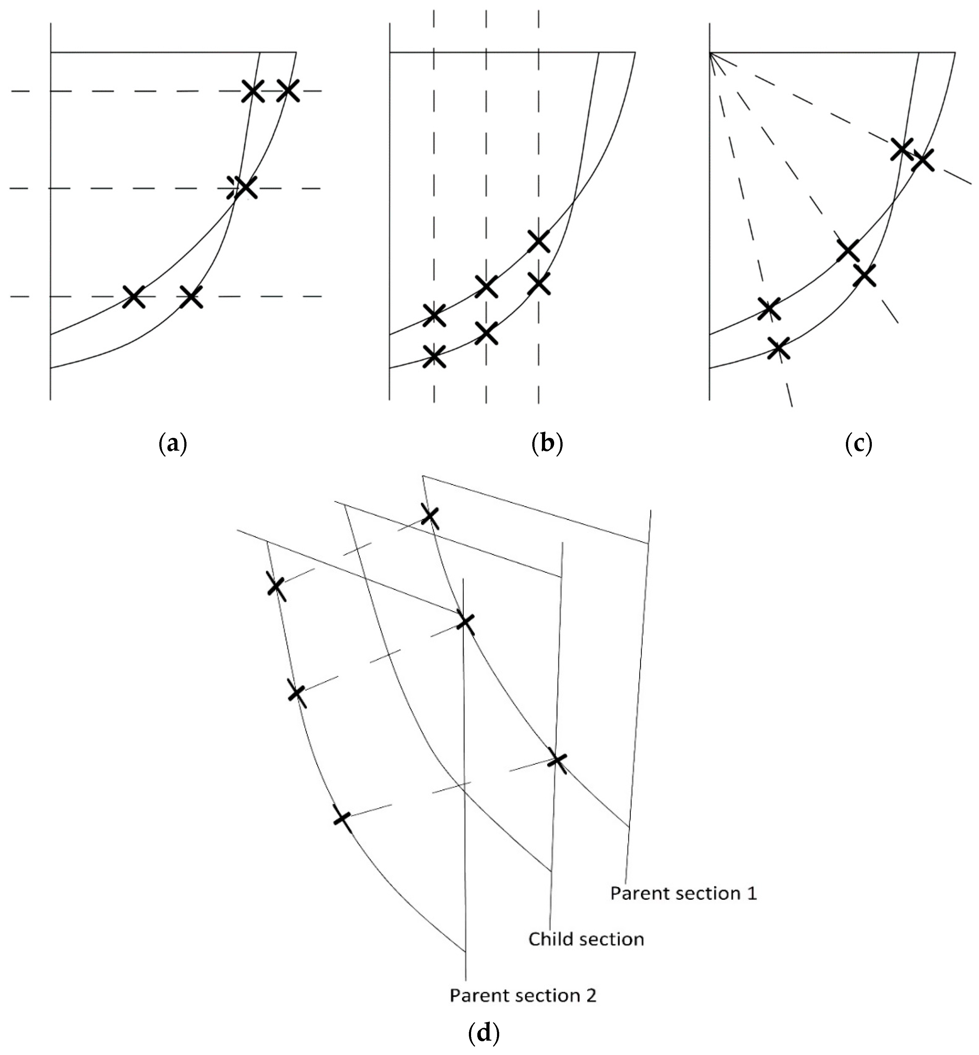
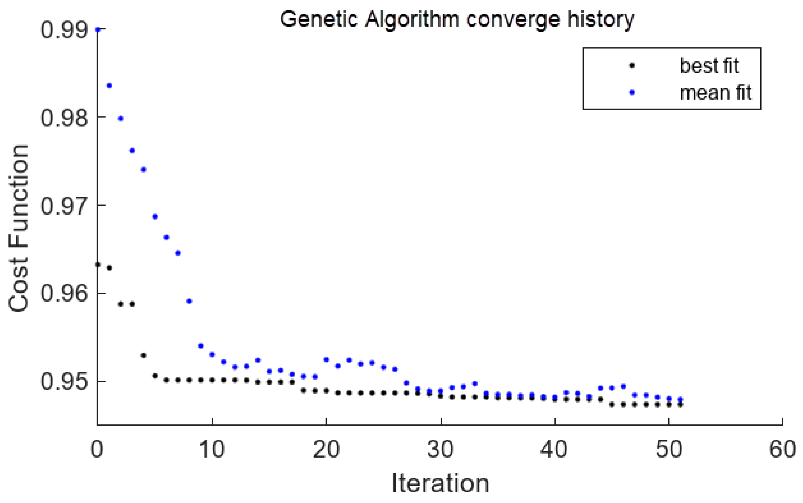
3.3. Genetic Algorithm Optimization

The Genetic Algorithm (GA) of the MATLAB optimization toolbox was used for direct optimization using the obtained resistance predictor. The genetic algorithm (GA) is an approach to optimization problems based on the mechanism of natural selection that underlies biological evolution. This algorithm iteratively adjusts a collection of individual solutions. At each iteration, the genetic algorithm selects specific individuals from the existing population to serve as parents, from which it generates offspring for the next generation. In subsequent iterations, the population undergoes an “evolutionary” development and converges to an optimal solution. The population size was selected as 40 with 100 Max Generations. Algorithm’s stopping or termination criterion is regulated via Max Generations and Max Stall Generations. The variable “Max Generations” denotes the upper limit of generations that process will go through during the optimization. The variable “Max Stall Genera-tions” represents the maximum number of consecutive generations in which there is no improvement in the best fitness value of the population. Max Stall Generations and Function tolerance are set to 50 and 0.005, respectively, to determine the stop condition. The algorithm terminates when the average relative change in the fitness function value over Max Stall Generations becomes smaller than the Function tolerance.

In the GA solver domain, there is a different treatment of linear constraints and bounds compared to nonlinear constraints. The optimization process ensures that all linear constraints and bounds are consistently satisfied. Nevertheless, it is important to note that the satisfaction of all nonlinear constraints may not be achieved in every generation during the GA operation.

In the case that the GA converges to a solution, the resulting solution is guaranteed to satisfy the requirements of the nonlinear constraints. In the genetic algorithm, three primary rule categories are employed during each iteration to generate the subsequent generation based on the existing population [33]:

▪

Selection rules select the individuals, called parents, that contribute to the population of the next generation. The selection depends on the individuals’ scores.

▪

Crossover rules combine two parents to form children for the next generation.

▪

Mutation rules apply random changes to individual parents to form children.

4. Results

Three regression models have been developed according to internal parameter selection to minimize the MSE value. The PCA dimensionality reduction reduces the number of features from nine to six features.

Table 4. Internal parameters of optimum regression models.

Optimizable Regression Tree	Optimizable Neural Network	Optimizable SVM
RMSE: 0.1043	RMSE: 0.03037	RMSE: 0.1168
R2: 0.98	R2: 1	R2: 0.97
MSE: 0.01088	MSE: 0.000922	MSE: 0.01365
MAE: 0.057334	MAE: 0.020429	MAE: 0.06614
Minimum leaf size: 3	Num. of layers: 2 Activation: Sigmoid Lambda: 1.5276 × 10−8 First Layer size: 26 Second Layer size: 77	Box constraint: 17.0223 Kernel scale: 8.5763 Epsilon: 8.17 × 10−4 Kernel function: Gaussian

presents evaluation results of the model performance and internal obtained parameters of regression models.

Regression evaluation results depict that the model developed using the artificial neural networks algorithm has been fitted more suitable than other implemented models. This model has an R-squared determination equal to 1, while the errors and dispersion measurements are minimal. Figure 4 illustrates the history of the MSE parameter minimization for three applied methods. The dark blue point corresponds to observed minimum MSE, and the light blue one represents the estimated minimum MSE. The number of iterations is considered 30, with the best point of MSE value shown in red color.

The response plot presented in Figure 5 shows the main and predicted responses versus the record number. Additionally, predicted vs. actual and residual plots are shown in Figure 6 for each regression model. These plots help us understand how well the regression model makes predictions for different response values. It can be indicated that the ANN method can predict responses close to the actual ones due to well-scattered samples along the diagonal line. Additionally, the residual plot depicts the difference between the predicted and true responses, which can be interpreted as a clear distribution around zero for the ANN regression method. In order to evaluate overfitting, 15% of samples were applied during regression modelling, and the RMSE of the validation value under training results is compared to the RMSE of the test value under test results, comprising 15% of the total samples. The assessment of response plots and modelling summary represents the appropriate performance of the ANN method against other implemented methods. In addition, the test RMSE is higher than the validation RMSE, which indicates that this model can be an appropriate resistance prediction model for the rest of the design study.

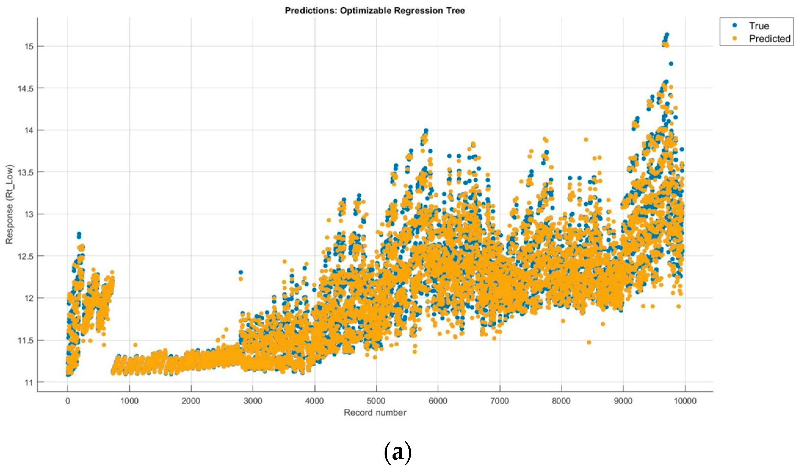
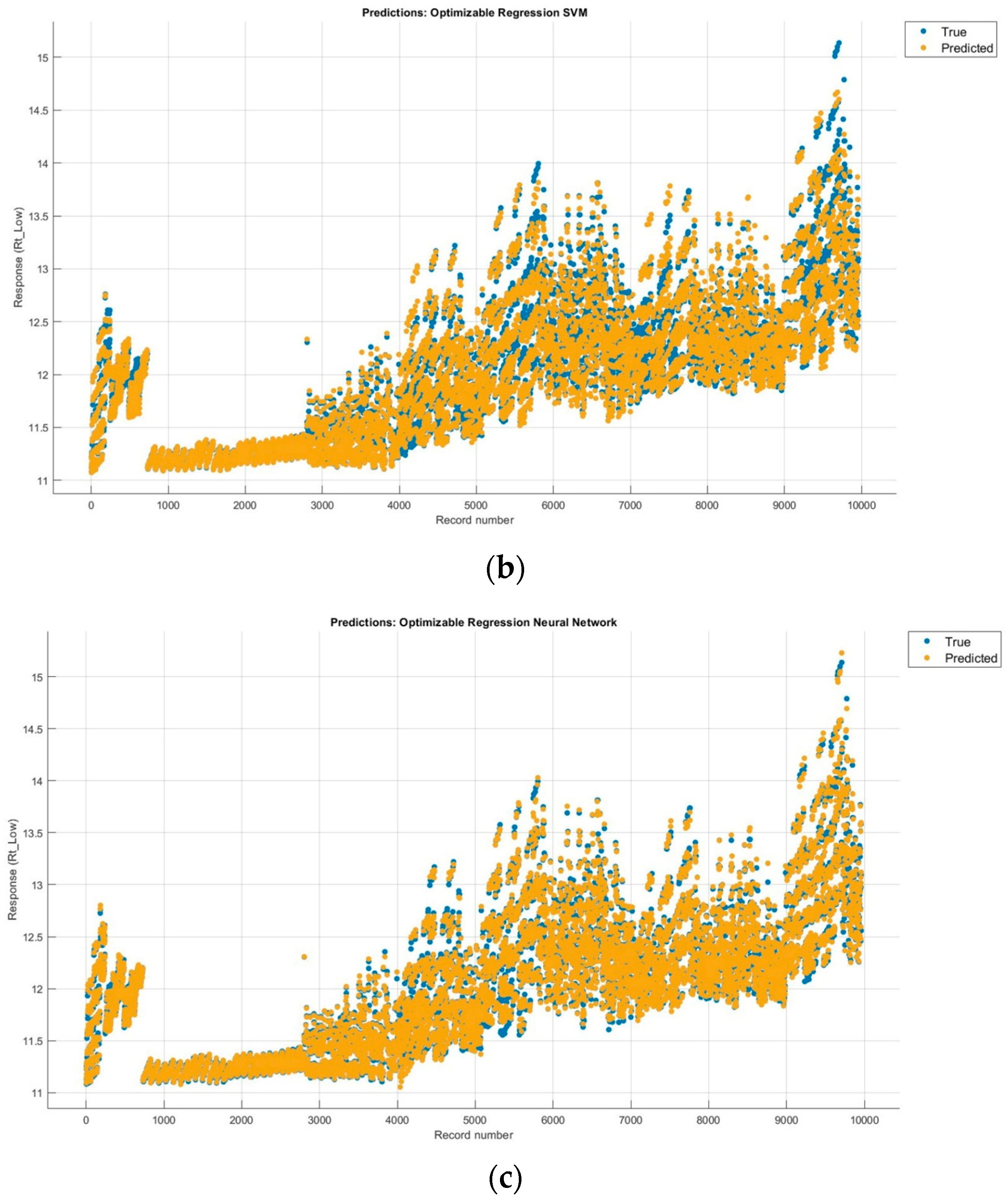
4.1. Regression Model Evaluation

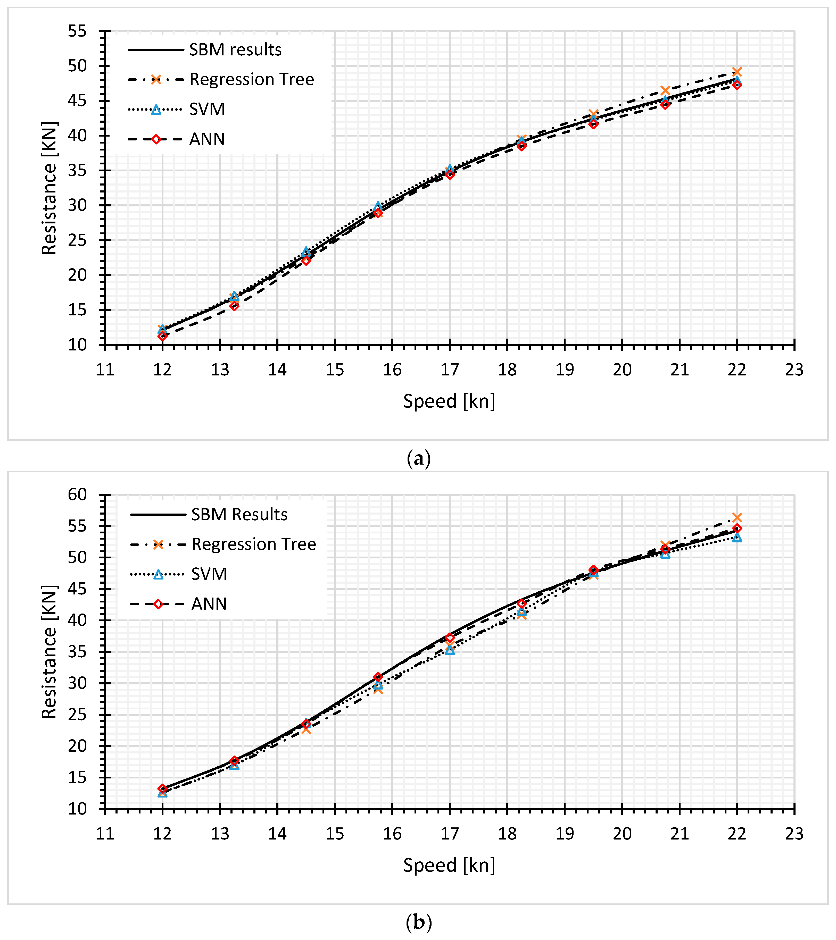
4.1.1. Dataset Test Cases

A comparison is conducted between RT, SVM, and ANN methods for evaluating resistance predictors. Two designs from the dataset have been selected randomly for evaluation in this subsection. Figure 7a shows the results for a random hull in the hullform series. In addition, Figure 7b depicts the results for a random catamaran hullform for the 85-ton series.

The proposed models fit well the observed data for test cases within the dataset. However, small underestimate values can be indicated at speeds 15 to 18 knots. R-square and RMSE values for Figure 7 (random design test model 1 and 2) are presented in

Table 5. Prediction parameters of the model test for dataset designs.

	Test Model 1	Test Model 2
RT	RMSE: 0.6051 R2: 0.9991	RMSE: 1.4895 R2: 0.9934
SVM	RMSE: 0.3185 R2: 0.9996	RMSE: 1.1625 R2: 0.9971
ANN	RMSE: 0.8083 R2: 0.9997	RMSE: 0.3606 R2: 0.9994

. The artificial neural networks algorithm fits the observed data effectively according to lower values of prediction parameters.

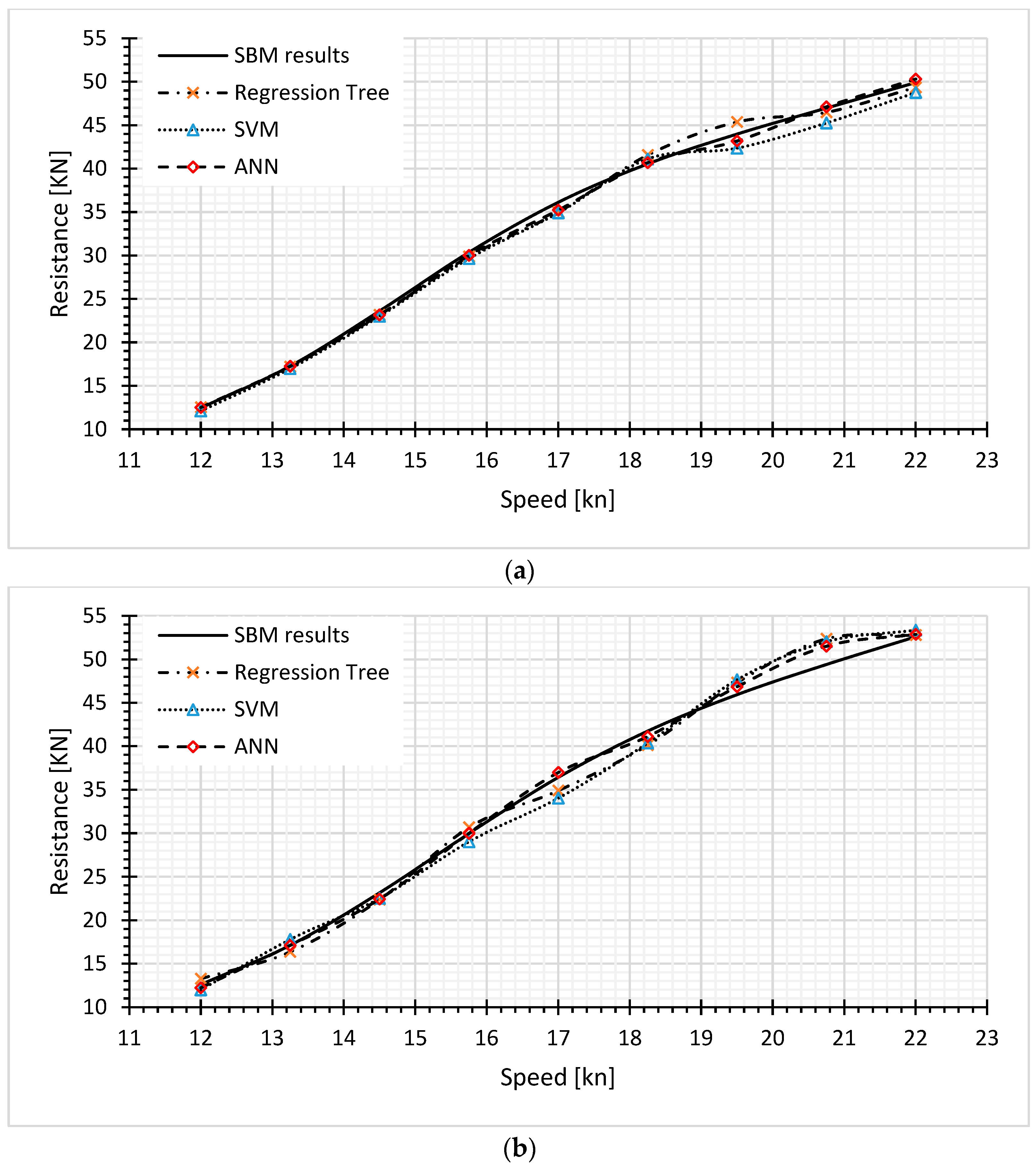
4.1.2. Interpolation Test Cases

In this section, two interpolated designs based on ship tonnage have been imported into regression models. Catamaran hullforms of 77.5 ton and 82.5 tons are designed for regression model evaluation. Three implemented regression models are adjusted for the 77.5-ton hullform (Figure 8a) and the 82.5-ton hullform (Figure 8b). Regression data are well adjusted using the ANN method for both designs according to predictor parameters presented in

Table 6. Prediction parameters of the model test for interpolation designs.

	77.5 ton	82.5 ton
RT	RMSE: 0.7597 R2: 0.9965	RMSE: 1.4029 R2: 0.9911
SVM	RMSE: 1.0426 R2: 0.9976	RMSE: 1.4938 R2: 0.9906
ANN	RMSE: 0.4677 R2: 0.9988	RMSE: 0.8633 R2: 0.9977

. However, a slight difference can be observed at higher speeds of the 82.5-ton case, which is slightly superior.

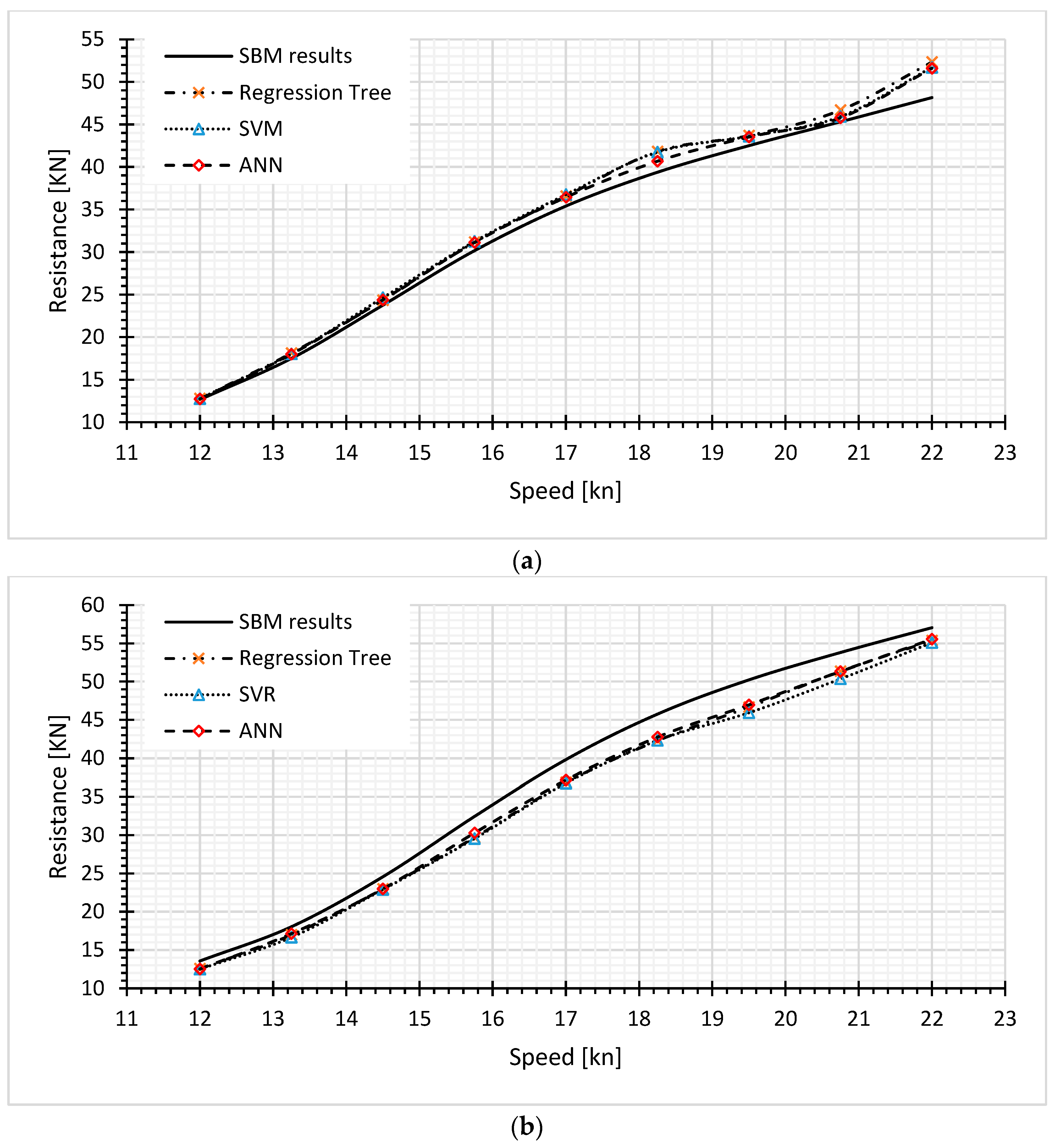
4.1.3. Extrapolation Test Cases

Extrapolation designs define hullforms outside the displacement bound of the dataset. Considering the displacement of all designs from the dataset are designed between 75 to 85 tons. two catamaran hullforms of 71.5 tons and 88.5 tons are considered for regression model evaluation. The purpose of the extrapolation test is the assessment of regression models for out-of-boundary catamarans. Figure 9a,b shows resistance values against speed for Slender Body Method results and fitted regressions for the 71.5-ton design and 88.5-ton design, respectively. In Figure 9a, all regression models estimate resistance higher than actual values. On the contrary, the proposed models are inferior to SBM results in Figure 9b. In the transition to high speeds, the models become less accurate. In addition,

Table 7. Prediction parameters of the model test for extrapolation designs.

	71.5 ton	88.5 ton
RT	RMSE: 1.8147 R2: 0.9964	RMSE: 2.4631 R2: 0.9975
SVM	RMSE: 1.6215 R2: 0.9965	RMSE: 2.7815 R2: 0.9975
ANN	RMSE: 1.3860 R2: 0.9968	RMSE: 2.2180 R2: 0.9983

presents prediction values of fitting quality, which depicts that regressions are more precise in the lower displacement design than in the higher one.

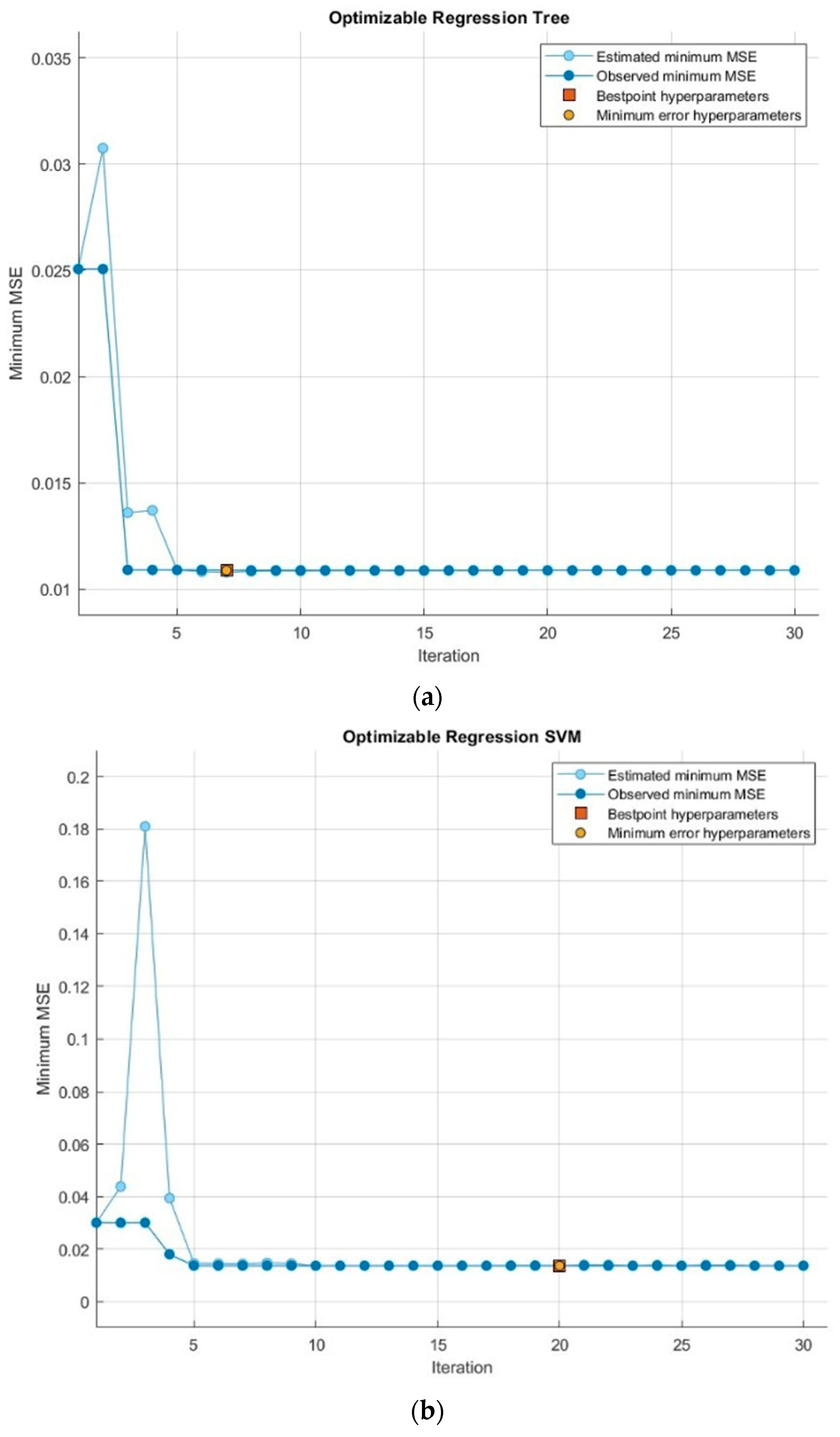
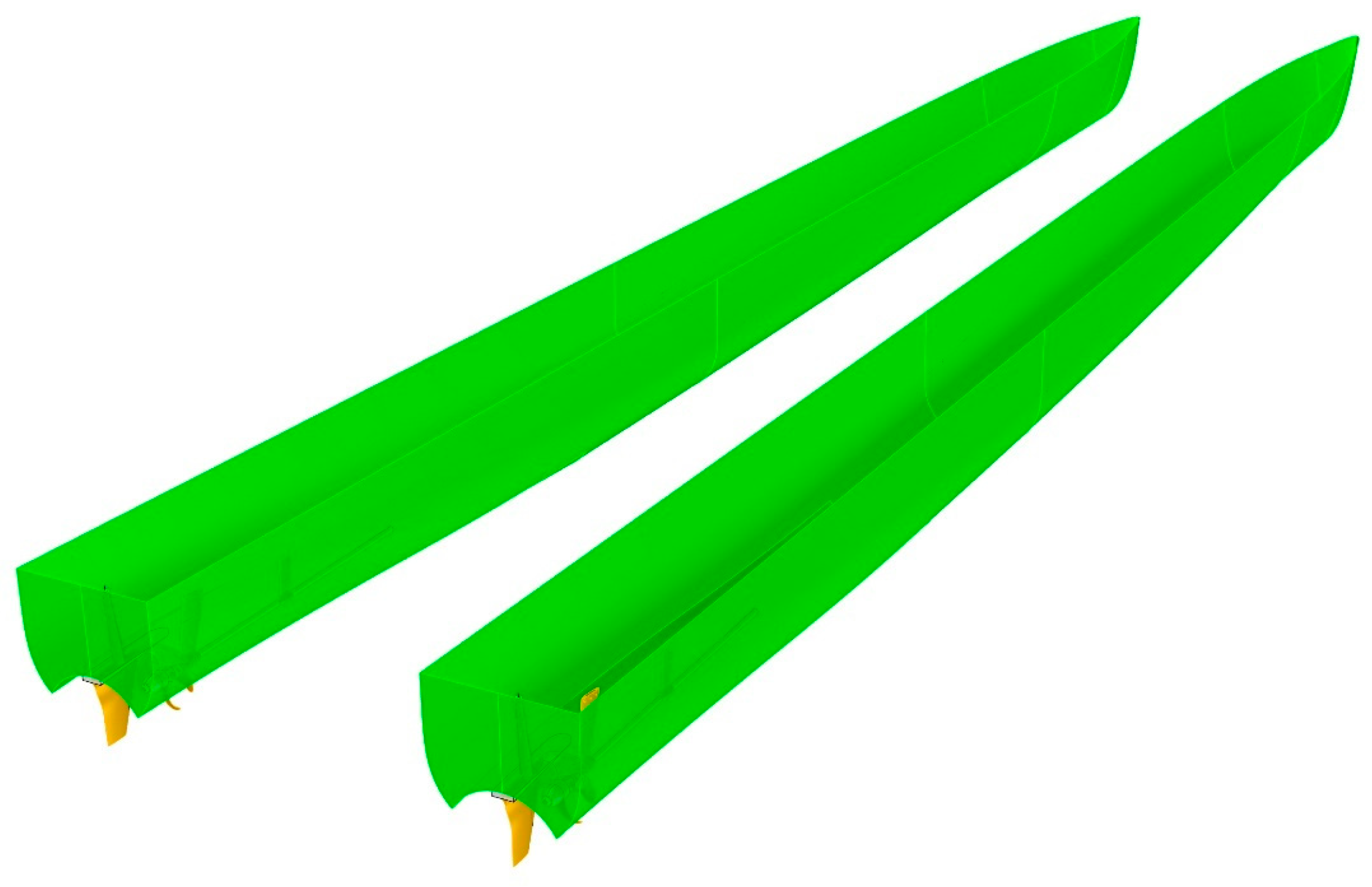
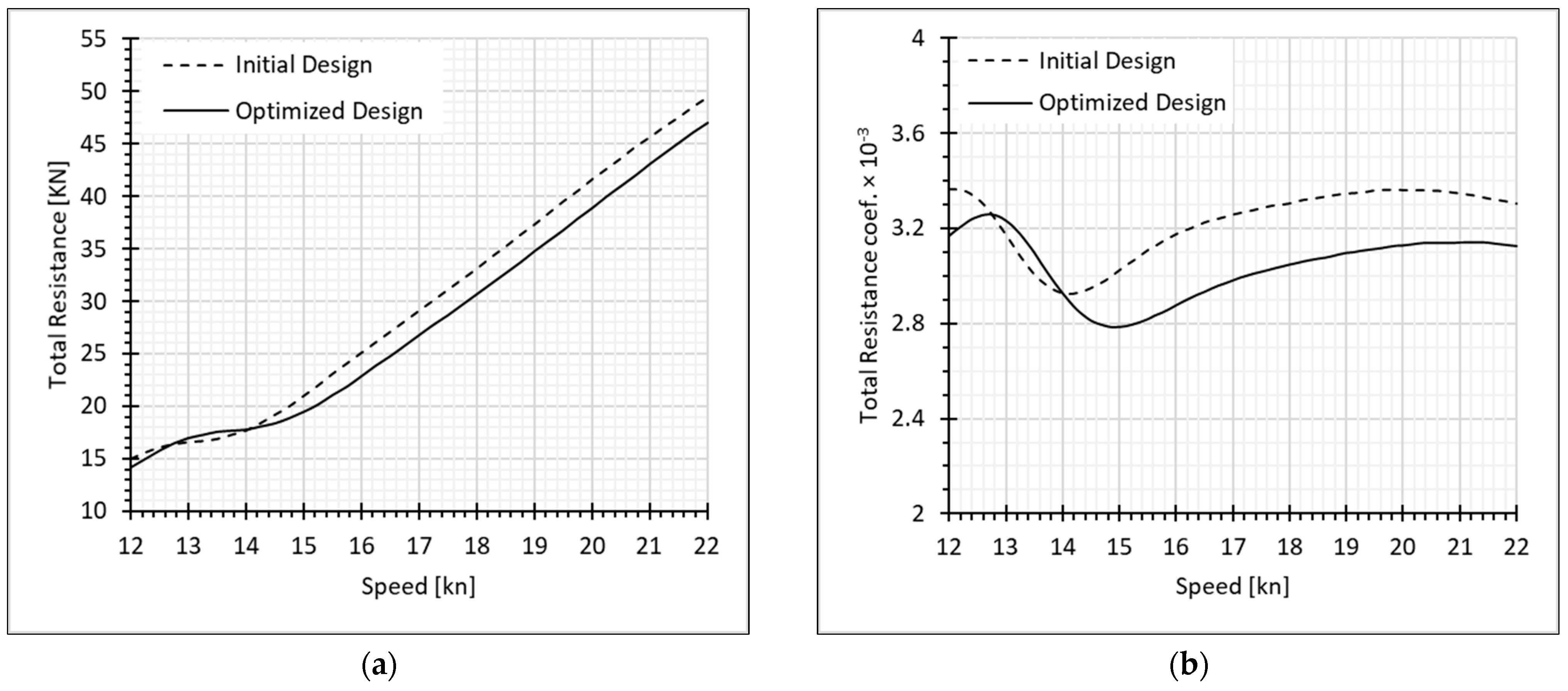
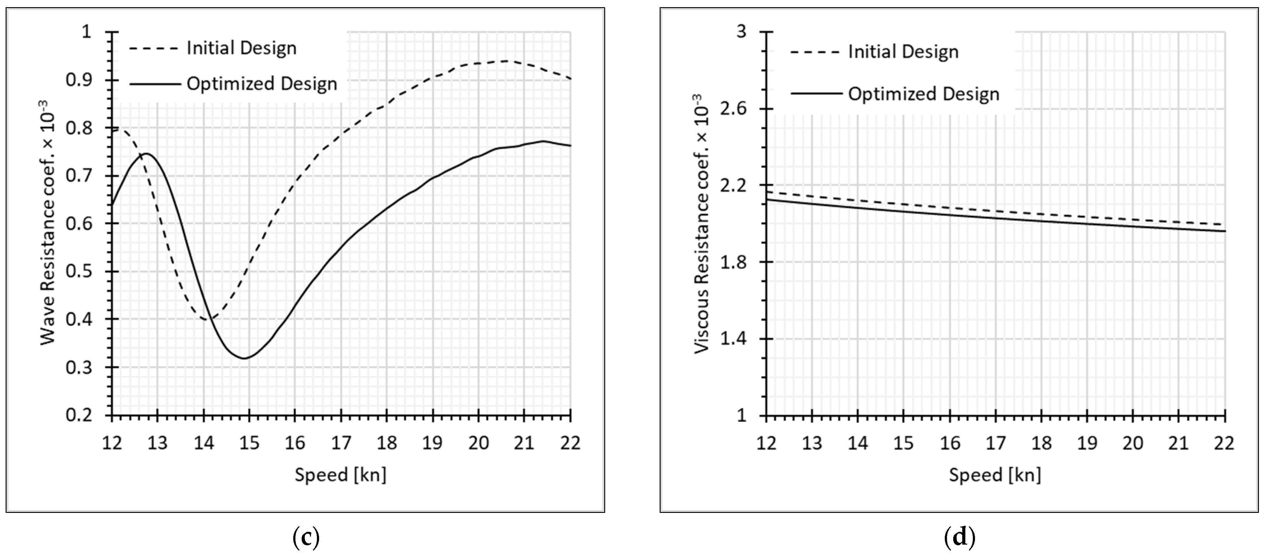
4.2. Genetic Algorithm Optimization

The optimization process is conducted for a 40 m catamaran to obtain the best design based on the defined cost function. The developed geometry reconstruction model offers the designer the possibility to control/specify the main particulars of the demi hull along with the hullform details within a reasonable range of variation of the defined design variables, while at the same time, ensuring adequate quality of fairness and smoothness of the hull. The Genetic algorithm parameters have been set up based on settings in Section 3.3.

Figure 10 illustrates a three-dimensional perspective of the TrAM catamaran hull, representing the initial hullform for the design optimization procedure. The design parameters for this investigation are presented in

Table 8. Design variables of the study.

Optimization Design Variables	Symbol	Min Bound	Max Bound
Waterline length (m)	Lwl	38	41
Demi hull Beam (m)	B	1.9	2.1
Draft (m)	T	1.1	1.15
Demi hull transverse distance (m)	DT	3.3	3.7
Block coefficient	Cb	0.49	0.53
Max section area coefficient	Cm	0.72	0.77
Prismatic coefficient	Cp	0.66	0.71
Longitudinal Center of Buoyancy (% of L)	LCB	0.51	0.56
Objectives & Constraints	Symbol	Min bound	Max bound
Resistance at two Ship speeds [kn]	V	12	22
Ship Light Weight (ton)	W	62.23
Ship Displacement (ton)	∆	90 ± 1%

, along with their corresponding ranges.

After 51 iterations the optimization terminates. The Genetic Algorithm convergence curve of the current study is shown in Figure 11. The best fit is the best design of each generation, and the mean fit is the average cost function of the population in each generation. Accordingly, 51 × 50 = 2550 designs have been generated in the GA optimization process by using a fast approach ML resistance predictor, which reduces computation cost to a few minutes.

The resistance value of the baseline design at a speed of 12 knots is 14.97 kN, and at speed 22 knots, it is 48.228 kN. According to Figure 12, the results of the optimization process on a 40 m passenger catamaran achieved a 12.2% resistance reduction at cruise speed and a 7.1% resistance reduction at sprint speed. In this Figure, each asterisk point represent best design of each generation during GA optimization process. By using Genetic Algorithm on a sample catamaran ship, it resulted in a 9.5% cost function improvement. Therefore, one can conclude that the developed in-house resistance predictor, combined with hullform optimization software, provides a superior and cost-effective solution for ship design. Resistance and cost function values and their corresponding improvements are presented in

Table 9. GA optimization results.

Design Study	Symbol	Original Catamaran Resistance [kN]	Optimized Catamaran Resistance [kN]	Improvement %
Genetic Algorithm	${Rt}_{Low}$ [kN]	14.97	13.183	12.20
	${Rt}_{High}$ [kN]	48.228	44.84	7.10
	CF	1	0.905	9.5

CF: Cost Function.

.

The final optimized catamaran from GA optimization has been obtained. A comparison of the initial and optimized values of ship attributes is illustrated in

Table 10. Principal dimensions of the initial and optimized catamaran hull.

Ship Principal Parameters	Symbol	Initial Design	Optimized Design
Waterline Length (m)	Lwl	39.80	41.0
Total demi hull Beam (m)	B	2.000	2.078
Draft (m)	T	1.100	1.110
Block coefficient	Cb	0.515	0.504
Midship coefficient	Cm	0.754	0.721
Prismatic coefficient	Cp	0.683	0.699
Demi Hull Distance (m)	DT	3.500	3.326
Longitudinal Centre of Buoyancy (m)	LCB (% of L)	46.59	44.52
Total breath (m)	(DT × 2) + B	9.00	8.73
Displacement (ton)	∇	90.00	89.23

$C_p=\frac{C_b}{C_m}$.

. It is indicated that the lengthening of the ship improves resistance and block coefficient, and the midship coefficient was reduced in the optimized design. The value for LCB is decreased, which can be inferred that a backward longitudinal displacement of the center of buoyancy position leads to a beneficial impact. Contrary to the fact, the demi hull distance was reduced from 3.5 to 3.326; one may conclude that the distance between demi hulls depends on the general configurator and ship hullform.

Figure 13 displays the body plan, and Figure 14 shows a perspective view of the initial and optimized hull. Evidently, it can be noticed that the length increases in the bow region of the optimized design. The obtained optimization results illustrate that the forward movement of the start point of the stern bottom improves hydrodynamic performance. The position of the profile view in the bow portion has been elevated, resulting in an alteration of the bow wave pattern.

Figure 15a illustrates the resistance plot corresponding to the ship’s velocity for both the initial and optimized hull configurations. Moreover, the graph displays the overall resistance, as well as the coefficients of wave-making and viscous resistance in Figure 15b, Figure 15c, and Figure 15d, respectively. These plots depict lower resistance and its component at different speeds except at speeds between 12.7 knots to 14 knots. The lower value of the wave-making resistance coefficient at hollow and hump regions can be concluded in Figure 15c, and these phenomena occur at speeds higher than initial design speeds.

As depicted in Figure 16a for the wave pattern surrounding the initial vessel and Figure 16b for the optimized vessel travelling at 12 knots, the calculated wave height around the hulls reflects the decrease in resistance. The optimized hull design results in diminished wave heights at the specified design velocities. The predominant alterations are enacted in the bow shape and the bottom of the stern region, leading to a decrease in wave heights in the middle and aft portions of the hull, as illustrated in Figure 16.

5. Conclusions

A systematic series of novel catamaran ships has been developed for two types of passenger and freight boats. Three different ship tonnages: 75, 80, and 85 tons, are considered to produce new designs. A shift transformation and self-blending method are sequentially applied to generate different hullforms. Three different supervised machine learning methods have been applied to the generated dataset of catamarans to predict resistance at different ship speeds. Accordingly, 9775 catamaran hullforms have been produced to create a vast optional condition for ship owners and provide this dataset for a machine learning resistance prediction model. Using machine learning algorithms, it is worth developing a continuous total resistance predictor well-fitted to the database of ship series. A highly significant concern is the huge time and cost of the optimization process, which herein we develop a machine learning resistance predictor that facilitates Genetic Algorithm optimization in an expedited manner. Three regression algorithms: Regression Tree, Support Vector Machine, and Artificial Neural Network approaches, are applied to the dataset. Regression estimation has good compliance with results of the SBM method at a wide range of speeds. However, RT and SVM methods have some differences in higher speed. The ANN approach depicts well-adjusted regression on the data. The validation of fitting methods was evaluated by case test of the dataset, interpolation, and extrapolation of catamarans. Accordingly, a general and unique tool is proposed to predict the resistance of the series at different displacements and hullforms. The proposed model is a valuable tool to assess the resistance of catamaran hulls during the early design stages. Finally, a sophisticated ANN model is proposed by exploring different features and training/optimization algorithms. A direct optimization algorithm (Genetic Algorithm) is applied for the optimization study. Waterline length, Demi hull breadth, ship draft, Demi hull offset distance, block coefficient, midship coefficient, prismatic coefficient, and longitudinal centre of buoyancy are design variables of the optimization study, considering total width and ship displacement as constraints of optimization. Total resistance at cruise and sprint speed and its light weight are the objectives of this study. The optimization process was conducted on a 40 m passenger catamaran that achieved a 12.2% resistance reduction at cruise speed and a 7.1% resistance reduction at sprint speed. The best approach is the Genetic Algorithm, which results in the highest resistance reduction, a 9.5% cost function improvement. For the optimized configuration, a reduction in wave amplitudes was observed at different design speeds, indicating the effects of the changes to the bow shape and lower stern area. Hence, it can be inferred that utilizing an internally developed resistance predictor in conjunction with hullform optimization software offers a superior and cost-efficient solution for ship design. The current approach can be extended to include additional objectives such as stability, seakeeping, and general arrangement. In addition, some non-linear design blending can be applied to hullform development to diversify the geometry of the ship, which can be carried out for future works.

References

1. Xing-Kaeding, Y.; Papanikolaou, A. Optimization of the Propulsive Efficiency of a Fast Catamaran. J. Mar. Sci. Eng. 2021, 9, 492. [Google Scholar] [CrossRef]
2. Wang, H.; Boulougouris, E.; Theotokatos, G.; Zhou, P.; Priftis, A.; Shi, G. Life Cycle Analysis and Cost Assessment of a Battery Powered Ferry. Ocean Eng. 2021, 241, 110029. [Google Scholar] [CrossRef]
3. Sarker, I.H. Machine Learning: Algorithms, Real-World Applications and Research Directions. SN Comput. Sci. 2021, 2, 160. [Google Scholar] [CrossRef]
4. Panda, J.P. Machine Learning for Naval Architecture, Ocean and Marine Engineering. J. Mar. Sci. Technol. 2023, 28, 1–26. [Google Scholar] [CrossRef]
5. La Ferlita, A.; Qi, Y.; Di Nardo, E.; Moenster, K.; Schellin, T.E.; EL Moctar, O.; Rasewsky, C.; Ciaramella, A. Power Prediction of a 15,000 TEU Containership: Deep-Learning Algorithm Compared to a Physical Model. J. Mar. Sci. Eng. 2023, 11, 1854. [Google Scholar] [CrossRef]
6. Cui, H.; Turan, O.; Sayer, P. Learning-Based Ship Design Optimization Approach. CAD Comput. Aided Des. 2012, 44, 186–195. [Google Scholar] [CrossRef]
7. Papanikolaou, A.; Xing-Kaeding, Y.; Strobel, J.; Kanellopoulou, A.; Zaraphonitis, G.; Tolo, E. Numerical and Experimental Optimization Study on a Fast, Zero Emission Catamaran. J. Mar. Sci. Eng. 2020, 8, 657. [Google Scholar] [CrossRef]
8. Nazemian, A.; Ghadimi, P. Shape Optimisation of Trimaran Ship Hull Using CFD-Based Simulation and Adjoint Solver. Ships Offshore Struct. 2022, 17, 359–373. [Google Scholar] [CrossRef]
9. Li, D.; Guan, Y.; Wang, Q.; Chen, Z. Support Vector Regression-Based Multidisciplinary Design Optimization for Ship Design. In Proceedings of the International Conference on Offshore Mechanics and Arctic Engineering-OMAE, Rio de Janeiro, Brazil, 1–6 July 2012; American Society of Mechanical Engineers: New York, NY, USA, 2012; Volume 1, pp. 77–84. [Google Scholar]
10. Fahrnholz, S.F.; Caprace, J.D. A Machine Learning Approach to Improve Sailboat Resistance Prediction. Ocean Eng. 2022, 257, 111642. [Google Scholar] [CrossRef]
11. Nazemian, A.; Ghadimi, P. Global Optimization of Trimaran Hull Form to Get Minimum Resistance by Slender Body Method. J. Braz. Soc. Mech. Sci. Eng. 2021, 43, 67. [Google Scholar] [CrossRef]
12. Margari, V.; Kanellopoulou, A.; Zaraphonitis, G. On the Use of Artificial Neural Networks for the Calm Water Resistance Prediction of MARAD Systematic Series’ Hullforms. Ocean Eng. 2018, 165, 528–537. [Google Scholar] [CrossRef]
13. Yao, J.; Han, D. RBF Neural Network Evaluation Model for MDO Design of Ship; International Proceedings of Computer Science and Information Technology (IPCSIT): Singapore, 2012; Volume 47, pp. 309–312. [Google Scholar]
14. Radojcic, D.V.; Morabito, M.G.; Simic, A.P.; Zgradic, A.B. Modeling with Regression Analysis and Artificial Neural Networks the Resistance and Trim of Series 50 Experiments with V-Bottom Motor Boats. J. Ship Prod. Des. 2014, 30, 153–174. [Google Scholar] [CrossRef]
15. Radojčić, D.V.; Kalajdžić, M.D.; Zgradić, A.B.; Simić, A.P. Resistance and Trim Modeling of a Systematic Planing Hull Series 62 (with 12.5°, 25°, and 30° Deadrise Angles) Using Artificial Neural Networks, Part 2: Mathematical Models. J. Ship Prod. Des. 2017, 33, 257–275. [Google Scholar] [CrossRef]
16. Cepowski, T. The Prediction of Ship Added Resistance at the Preliminary Design Stage by the Use of an Artificial Neural Network. Ocean Eng. 2020, 195, 106657. [Google Scholar] [CrossRef]
17. Kim, J.H.; Kim, Y.; Lu, W. Prediction of Ice Resistance for Ice-Going Ships in Level Ice Using Artificial Neural Network Technique. Ocean Eng. 2020, 217, 108031. [Google Scholar] [CrossRef]
18. Liu, S.; Papanikolaou, A. Regression Analysis of Experimental Data for Added Resistance in Waves of Arbitrary Heading and Development of a Semi-Empirical Formula. Ocean Eng. 2020, 206, 107357. [Google Scholar] [CrossRef]
19. Priftis, A.; Boulougouris, E.; Turan, O.; Atzampos, G. Multi-Objective Robust Early Stage Ship Design Optimisation under Uncertainty Utilising Surrogate Models. Ocean Eng. 2020, 197, 106850. [Google Scholar] [CrossRef]
20. Shi, G.; Priftis, A.; Xing-Kaeding, Y.; Boulougouris, E.; Papanikolaou, A.D.; Wang, H.; Symonds, G. Numerical Investigation of the Resistance of a Zero-Emission Full-Scale Fast Catamaran in Shallow Water. J. Mar. Sci. Eng. 2021, 9, 563. [Google Scholar] [CrossRef]
21. Aung, M.Z.; Nazemian, A.; Boulougouris, E.; Wang, H.; Duman, S.; Xu, X. Establishment of a Design Study for Comprehensive Hydrodynamic Optimisation in the Preliminary Stage of the Ship Design. Ships Offshore Struct. 2023, 18, 1–14. [Google Scholar] [CrossRef]
22. Boulougouris, E.; Priftis, A.; Dahle, M.; Tolo, E.; Papanikolaou, A.; Xing-Kaeding, Y.; Jürgenhake, C.; Svendsen, T.; Bjelland, M.; Kanellopoulou, A.; et al. TrAM-Transport: Advanced and Modular. In Proceedings of the 8th Transport Research Arena TRA 2020, Helsinki, Finland, 27–30 April 2020; pp. 1–10. [Google Scholar]
23. Couser, P.R.; Wellicome, J.F.; Molland, A.F. An Improved Method for the Theoretical Prediction of the Wave Resistance of Transom-Stern Hulls Using a Slender Body Approach. Int. Shipbuild. Prog. 1999, 45, 331–349. [Google Scholar]
24. Maxsurf Modeler, Maxsurf Resistance, and Automation, User Guide. Available online: https://communities.bentley.com (accessed on 22 February 2023).
25. Lackenby, H. On the Systematic Geometrical Variation of Ship Forms. Trans. R. Inst. Nav. Archit. 1950, 92, 289–316. [Google Scholar]
26. Roh, M.-I.; Lee, K.-Y. Computational Ship Design; Springer: Singapore, 2018; ISBN 978-981-10-4884-5. [Google Scholar]
27. Hotelling, H. Analysis of a Complex of Statistical Variables into Principal Components. J. Educ. Psychol. 1933, 24, 417–441. [Google Scholar] [CrossRef]
28. Tukey, J.W. John W. Exploratory Data Analysis/John W. Tukey; Addison-Wesley series in behavioral science; Addison-Wesley Pub. Co.: Reading, MA, USA, 1977; ISBN 0201076160. [Google Scholar]
29. Zaki, M.J.; Meira, W., Jr. Data Mining and Machine Learning; Cambridge University Press: Cambridge, UK, 2020; ISBN 9781108564175. [Google Scholar]
30. Aggarwal, C.C. Data Mining: The Textbook; Springer: Berlin/Heidelberg, Germany, 2015; Volume 1. [Google Scholar]
31. Riedmiller, M.; Braun, H. A Direct Adaptive Method for Faster Backpropagation Learning: The RPROP Algorithm. In Proceedings of the IEEE International Conference on Neural Networks, San Francisco, CA, USA, 28 March–1 April 1993; IEEE: Piscataway, NJ, USA, 1993; pp. 586–591. [Google Scholar]
32. The Mathworks Inc. Statistics and Machine Learning Toolbox Documentation. Available online: https://www.mathworks.com/help/stats/index.html (accessed on 16 June 2023).
33. The MathWorks Inc. MATLAB- Optimization Toolbox, Version 6.2. Available online: http://www.mathworks.com/products/optimization/ (accessed on 22 June 2023).
Figure 1. General arrangement plan of passenger and freight catamaran boats.
Jmse 12 00216 g001
Figure 2. Framework of machine learning and design optimization methodology.
Jmse 12 00216 g002
Figure 3. Self-blending of section control points: (a) YZ waterline intersection, (b) YZ Buttock line intersection, (c) YZ diagonal intersection, (d) X direction section blending.
Jmse 12 00216 g003
Figure 4. MSE history reduction through the optimizable regression process: (a) Regression Tree, (b) Regression SVM, (c) Regression ANN.
Jmse 12 00216 g004aJmse 12 00216 g004b
Figure 5. Prediction vs. true design comparison through the optimizable regression process: (a) Regression Tree, (b) Regression SVM, (c) Regression ANN.
Jmse 12 00216 g005aJmse 12 00216 g005b
Figure 6. Residual plot comparison through the optimizable regression process: (a) Regression Tree, (b) Regression SVM, (c) Regression ANN.
Jmse 12 00216 g006aJmse 12 00216 g006b
Figure 7. Model comparison between RT, SVM, and ANN methods for (a) random design Test model 1 and (b) random design Test model 2.
Jmse 12 00216 g007
Figure 8. Model comparison between RT, SVM, and ANN methods for (a) interpolation design, 77.5 tons and (b) interpolation design, 82.5 tons.
Jmse 12 00216 g008
Figure 9. Model comparison between RT, SVM, and ANN methods for (a) extrapolation design, 71.5 tons and (b) extrapolation design 88.5, tons.
Jmse 12 00216 g009
Figure 10. 3D view of the passenger catamaran.
Jmse 12 00216 g010
Figure 11. Genetic Algorithm convergence curve.
Jmse 12 00216 g011
Figure 12. Genetic Algorithm best design distribution of 51 generations.
Jmse 12 00216 g012
Figure 13. Body plan comparison of the initial and optimized hulls.
Jmse 12 00216 g013
Figure 14. 3D view comparison of the initial and optimized hulls.
Jmse 12 00216 g014
Figure 15. Comparison of total resistance (a), total resistance coefficient (b), wave-making resistance coefficient (c), and viscous resistance coefficient (d) at different speeds between the initial and optimized design.
Jmse 12 00216 g015aJmse 12 00216 g015b
Figure 16. Comparison of wave pattern at (a) Initial design at 12 knots, (b) Optimized design at 12 knots, (c) Initial design at 22 knots, (d) Optimized design at 22 knots.
Jmse 12 00216 g016