Abstract
The NACRA 17 is a small foiling catamaran that is lifted out of the water by two asymmetric z-foils and two rudder elevators. This paper investigates how foil deflection affects not only foil performance but overall boat behaviour using a numerical Fluid Structure Interaction (FSI) model. The deformations are solved with a solid model based on the Finite Element Method (FEM) and the flow is solved with a Reynolds Average Navier-Stokes (RANS) based Finite Volume Model (FVM). The models are strongly coupled to allow dynamic FSI simulations. The numerical model is validated by comparing it to an experimental campaign conducted at the RISE SSPA Maritime Center in Sweden.Validation shows reasonable agreement, but the model can only be considered validated for some rake angles. The large deformation of the foils is found to have a profound effect on the performance of the foils and therefore of the overall catamaran. Turbulence transition and boat speed are found to affect foil forces and, in turn, deformation. Dynamic response of the foils during boat motion as exposed to waves is investigated and finally the full boat hydrodynamic is simulated by including both foils and the rudders in various scenarios.
1. Introduction
Foiling boats has gained significant interest in recent years driven by development in Americas cup, Olympic sailing, and even offshore racing. The number of boats that are partly or fully foiling increase every year. The increased popularity of foiling boats increases the need to understand and simulate how the foils work. Much effort has been put into predicting hydrodynamic performance both numerical and experimental. Modern hydrofoils are thin to reduce drag and the tin structure results in large deformations during sailing and therefore Fluid Structure Interaction (FSI) are important. In recent years much work has been published on FSI of foils, see for example [1,2,3,4,5,6,7,8,9,10,11,12].
1.1. The Boat
The NACRA 17 is a small (5.25 m hull length) 2-person foiling catamaran used for Olympic competition that can sail at high speeds, with top speeds approaching 27 knots [13]. The boat is lifted out of the water by two asymmetric z-foils and two rudder elevators, all four foils can be independently adjusted in rake angle, with the z-foils ranging between −2.0° to +5.5° and the rudders having an overall total range of movement of 4.5° over their span. The z-foils are thin and slender and despite the stiff carbon fibre construction they experience large deformations when subject to sailing loads.
The deformation of the foils changes the direction of the lift force and this changes how much of the lift is keeping the boat foiling and how much prevents the boat from sailing side ways. Therefore, deformations affect the the whole balance of the boat.
1.2. State of the Art
To solve this highly coupled FSI problem a detailed model of the fluid flow and solid is required. It is common to use a Finite Element Model (FEM) to solve the solid problem. The complexity of the models varies from simple beam elements [1,3,5,7,9,10,11,12] to the more complex shell [6,7,8,9] and solid elements [2] and in some cases even considering anisotropic material properties. The fluid flow problem can also be solved with varying degrees of complexity from lifting line method [3,12] to unsteady Reynolds Average Navier-Stokes (RANS) Finite Volume Methods (FVM) [6]. The advantage of a simple method like lifting line is short computational time, but the simplicity of the model fails to represent the physics of the problem in detail. More details on fluid flow models for foils can be found in [14]. Some studies [2,7,9] found bend-twist coupling of the foils to be important. Experience with large flow induced deformation of thin structures can also be found on the aerodynamic of sailing boats, where recent work [15,16,17,18,19] investigated FSI simulation of yacht sails.
Coupling between solid and fluid model must be two-way, because the deformations due to fluid forces is large enough to impact the flow significantly. The significant unsteady deformation of the foils when exposed to waves and motions further require a strong coupling where information is exchanged multiple times within a time step.
Most of the previous work focus either on complex models to solve FSI for a simplified problems, such as a small part of the foil in a water tunnel [4,6,7], or a simplified model to solve the complex problem to reduce computational time [3,5,7]. One of the limitations of the complex dynamic FSI models is that the time step of the models needs to be very low and the number of iterations per time step needs to be large to maintain stability. The very low time step combined with large computation timer per time step makes solution of longer time series impractical. More detail on the topic can be found in [20].
1.3. Present Work
In the present work both solid and fluid flow models are created in the commercial software package STAR-CCM+ ver. 2310 from SIEMENS. The solid model is based on solid FEM and the fluid flow model is based on RANS FVM. The work is an extension of the work presented in [8,14,20]. In [8] FSI of the NACRA 17 foil is investigated both experimental and numerical. The experimental investigation are used also in the present paper for validation. The numerical work uses RANS for fluid part and shell FEM in Abaqus for the structural part. The computation focus on steady forces although an unsteady solver is used. The present work focus on dynamics of the FSI. Unlike other studies [3,5,7] where simple models are used to reduce complexity for longer transient runs the present work seeks to keep the high fidelity models for all simulations. By keeping all simulations in the same program, the stability of the solution is enhanced, and this enables use of higher time steps and fewer inner iterations.
1.4. Validation
The numerical model is validated by comparing it to an experimental campaign conducted at RISE SSPA Maritime Center in Sweden. In this experiment, described in detail in [8], the NACRA 17 z-foil is mounted in a water tunnel exposed to high flow speeds, representative of sailing loads, while forces and deflection are monitored. Furthermore, the numerical model is verified by detailed mesh studies of both solid model and fluid flow model.
1.5. Investigations
This paper, after validating the numerical simulations, investigates how foil deflection affects not only foil performance but also the overall boat behaviour and how the wakes coming off the front z-foils affect the rudders behaviour, analysing also the effects of wake on rudder’s toe-in or toe-out angles. The investigation can help understand the physics of the foil and why the boat behaves as it does. Through this understanding better boat setup and handling can be obtained. The NACRA 17 is dynamic while sailing and small changes in environmental conditions can lead to large motions of the boat. Especially waves can make sailing the boat in flying mode challenging. A typical Mistral day in the bay of Marseille, the 2024 Olympic venue, has been chosen for waves simulations. When waves are hitting the foils, as described in the latter part of the paper, the boat is experiencing large motions and the loads on the foils can change rapidly with large corresponding variations in deflection of the foils.
2. Methods
In this section the numerical FSI model is described along with a short description of the experiments used for tuning and validation. The model is increasing in complexity throughout the paper with the addition of the NACRA 17 rudders and the second foil, however, the prominent part of the work considers the behaviour and the fluid structure interaction of a single NACRA 17 z-foil. There are different models used for different cases in the work and this is highlighted below in the individual sections.
2.1. Solid Model
To solve the deformation of the foil under loading a FEM is used. In this section the model is described and in Section 3.1.1 the model is verified by a mesh convergence study and tuned to match structural test results.
2.1.1. Solid Geometry and Boundary Conditions
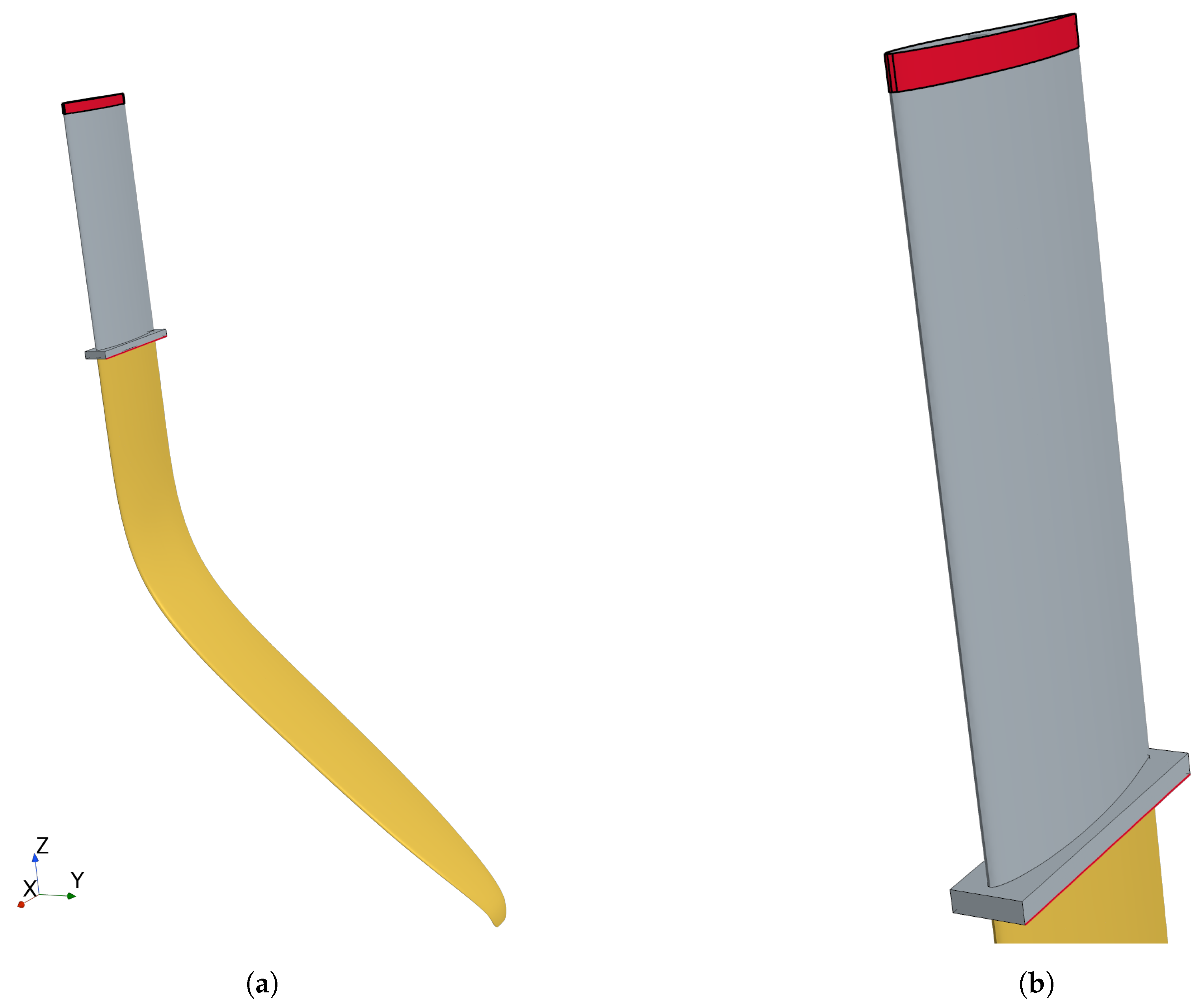
The outer geometry of the foil, shown if Figure 1, is based on a 3D scanning and CAD reconstruction further described in [14]. Most of the foil has a constant chord length of 200 mm and this is used as reference chord length c throughout the paper. For the solid model an estimate of the internal structure is required as the NACRA 17 is a one-design class and the structural properties are not released to the public. The foil is expected to consist of an outer sheet of varying thickness and an internal stiffener. The thickness of the sheet is measured at different chord-wise positions using an ultra sonic scanner. Three different foils have been scanned (serial numbers ZS00237, THB21887, and THC21879), and averaged values are used for the creation of the section geometry. The resulting section geometry can be seen in Figure 2a. Thickness is measured at a single span-wise location, and it is assumed that the thickness is uniform in the entire span. This is a crude approximation since the layers are expected to taper of towards the tip. Figure 1 shows the outer foil geometry for the solid model. The yellow part is the interface to the fluid model and the red parts represent the constraints of the solid model. At the top the foil is constrained in all directions, while the bottom constraint allows for rotation about the red line to represent the freedom of motion in the foil system of the boat. In the validation case in the cavitation tunnel the mount is slightly different as the foil is clamped also at the bottom constraint preventing rotations.

Figure 1.
NACRA 17 foil geometry for solid model. The interface to the fluid model is highlighted in yellow, and the constraints of the solid model are highlighted in red: (a) overview; (b) zoom.

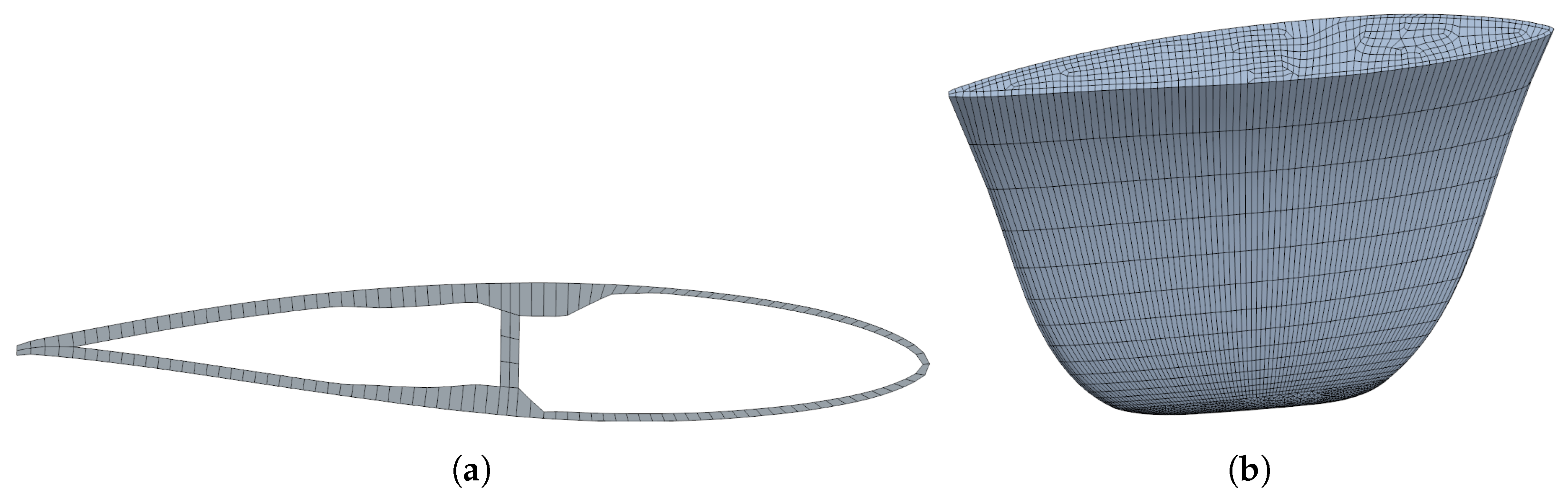
Figure 2.
Solid model mesh: (a) cross section; (b) mesh of tip section.
2.1.2. Solid Mesh
The mesh is a structured mesh for most of the foil with 2nd order 20 node hexagonal solid elements created by the directed mesh approach. For more details on element types see [20]. There are 76 elements in the chord direction, one element in the thickness and 200 elements in the span. The cross section of the mesh is shown in Figure 2a. The tip of the foil is modelled as a solid and split in two parts for meshing. The first part is meshed as a directed mesh with an unstructured source mesh and the second part at the very tip of the foil is meshed with an 3D unstructured mesh because of its complex shape. The tip parts contain both hexagonal, wedge, and pyramid shaped 2nd order elements as shown in Figure 2b. A total of 49,050 elements are used with 278,471 nodes.
2.1.3. Solid Models and Solvers
For the main part of the work an implicit unsteady solver is used with generalized- 2nd order accurate time integration. For the validation case a steady state solver is used. Due to large deformations non-linear geometry representation is utilized and the stiffness matrix is updated at every iteration. The linear system is solved by a hybrid MUltifrontal Massively Parallel sparse direct Solver (MUMPS) [21]. The material of the foil is carbon fibre reinforced epoxy that can have anisotropic properties, but in the present study it is assumed isotropic. The material properties are found by tuning to the experiment described in Section 2.4 and the material properties used are summarized in Table 1.

Table 1.
Material properties used for the solid model. denotes density, E is Youngs modulus and is Poisson’s ratio.
2.2. Fluid Flow Model
In this section the fluid flow model is described. It is based on RANS with finite volume discretisation. There are three different models with variation of domains and boundary conditions. The first is the validation model where the flow is modelled inside the cavitation tunnel. In this case no free surface is present and therefore the problem can be solved as steady state. In all other cases the water surface is included, and this requires an unsteady solution.
2.2.1. Geometry of Flow Domain and Boundary Conditions
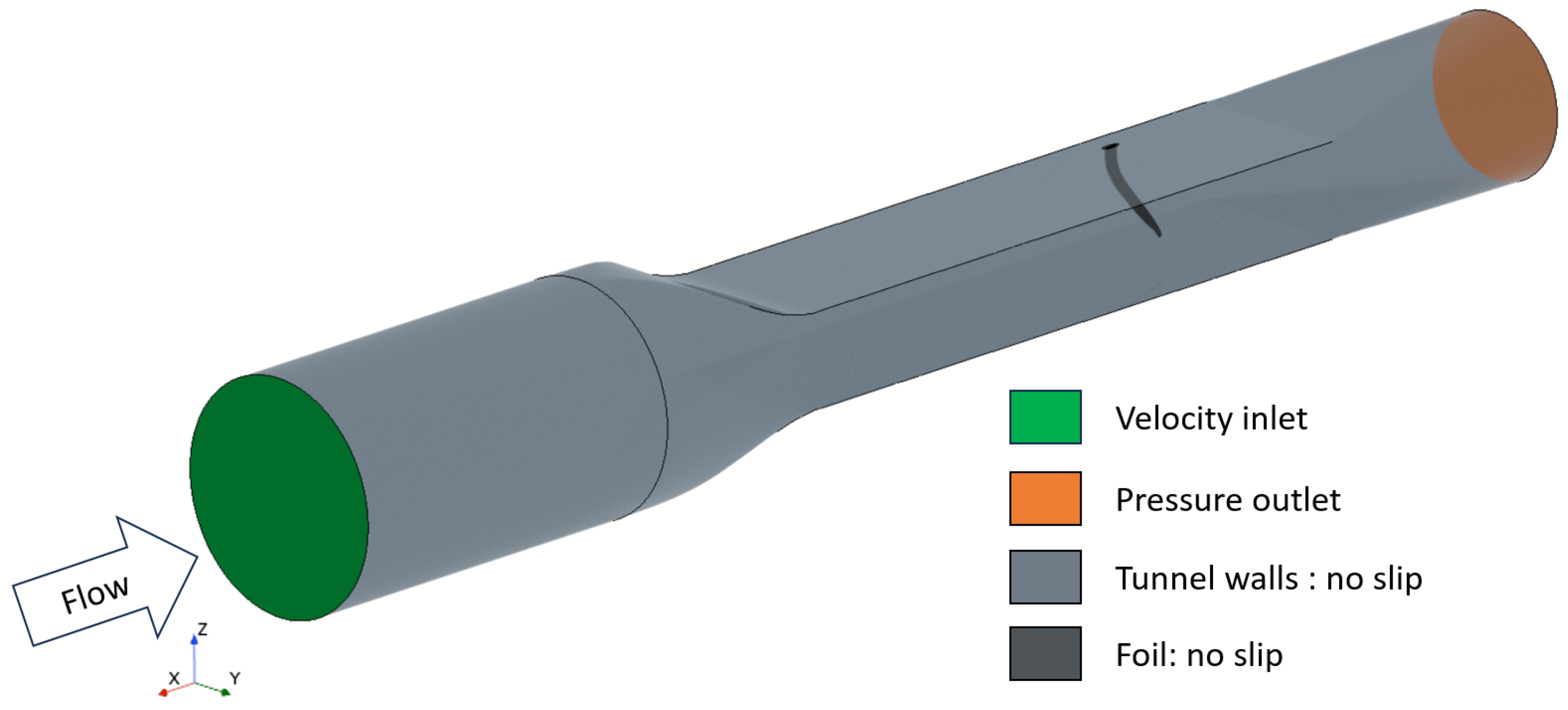
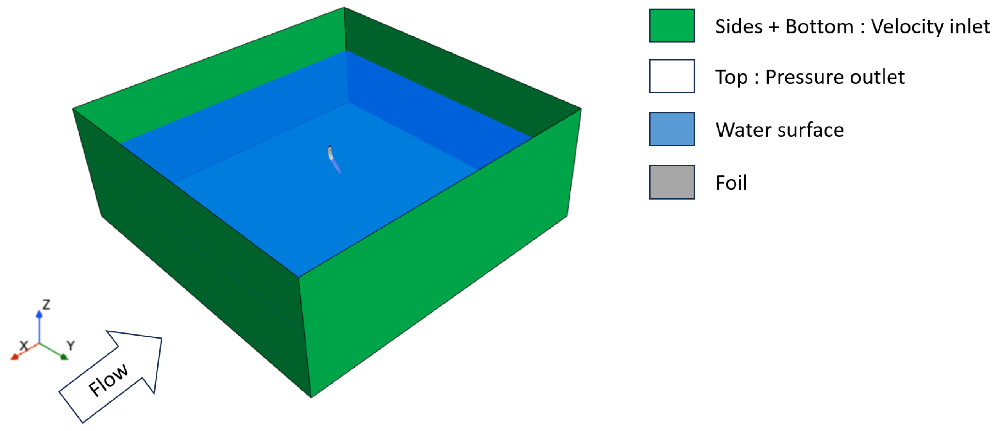
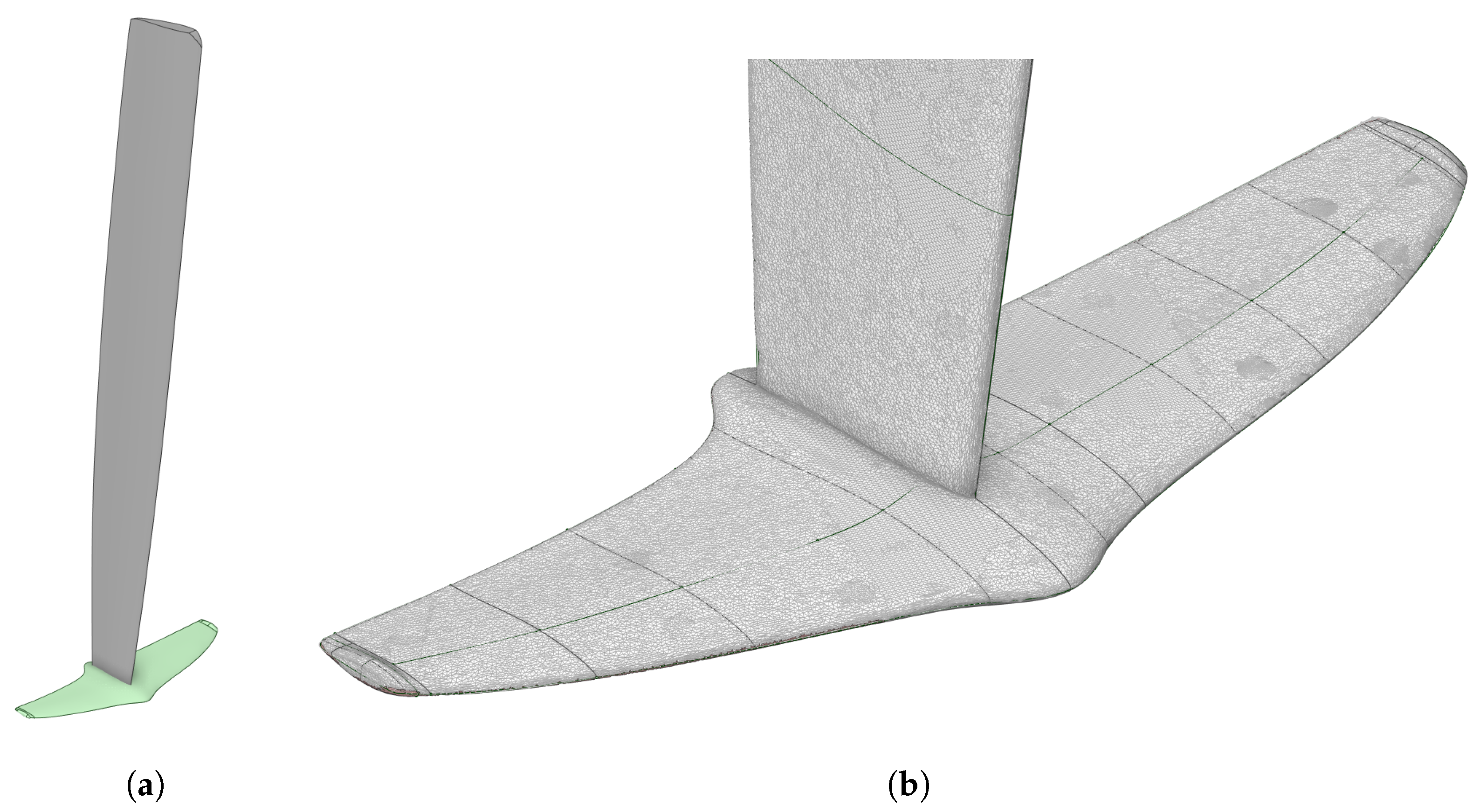
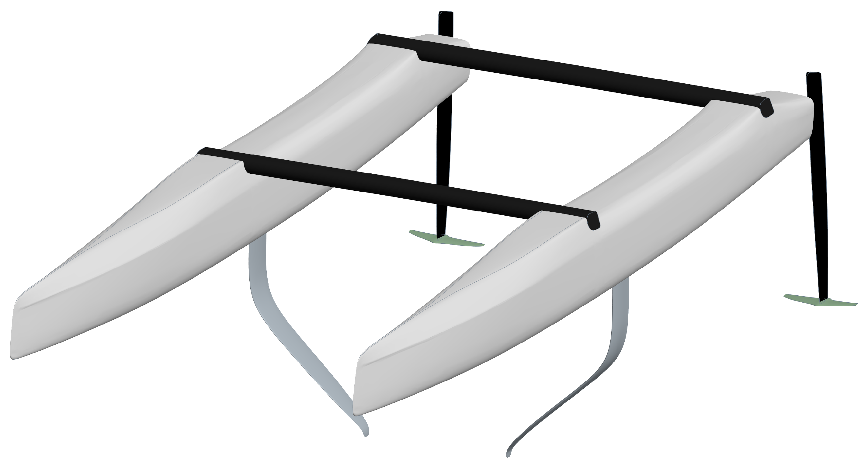
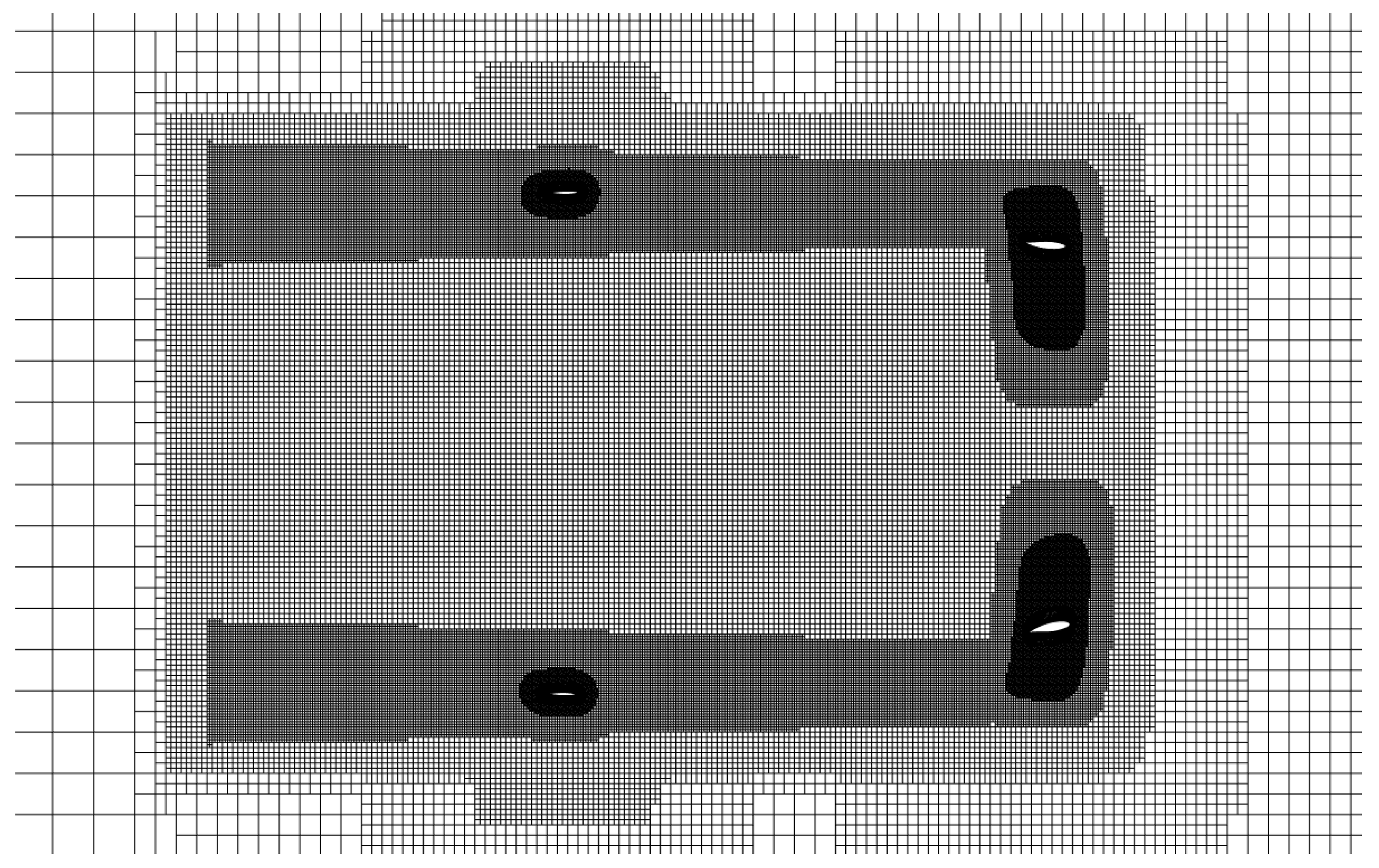
The same basic CAD model as described in Section 2.1.1 is used for the flow model. The surrounding domain is different for the different models as listed in Table 2. For the validation model a CAD model of the water tunnel as shown in Figure 3 is included to represent the flow conditions in the experiment as closely as possible. The inlet of the cavitation tunnel is extended 5 m upstream to avoid separation zones near the inlet. To simulate the foil sailing in open water a square domain including both water and air is used. The square domain extends 8 m from the foil in in all directions in the horizontal plane and 4 m in vertical direction as shown in Figure 4. The top of the square domain is a pressure outlet and all other exterior surfaces are velocity inlets. This configuration is chosen to effectively include waves in the model. In simulations including both foils and rudder the domain is extended by another 2 m in all directions to ensure sufficient distance to the boundary for both foils and rudders. The flow on the rudders are modelled in a similar way as the foil, but deformation are not included. The rudder and elevators are scanned with a structured light scanner and the CAD shown in Figure 5a is reconstructed based on the scanning. Figure 5b shows the rudder elevator mesh from the scanning with construction lines for reconstruction. The boat with both rudders and foils is shown in Figure 6. The hulls and cross beams are only shown for illustration and are not included in the computations.
Table 2.
Simulation models, settings and cells.

Figure 3.
Cavitation tunnel domain.

Figure 4.
Domain for foil performance simulations.

Figure 5.
Rudder and elevator: (a) CAD model; (b) zoom of elevator mesh from scanning and reconstruction curves.

Figure 6.
Boat geometry including rudders and foils.
2.2.2. Fluid Mesh
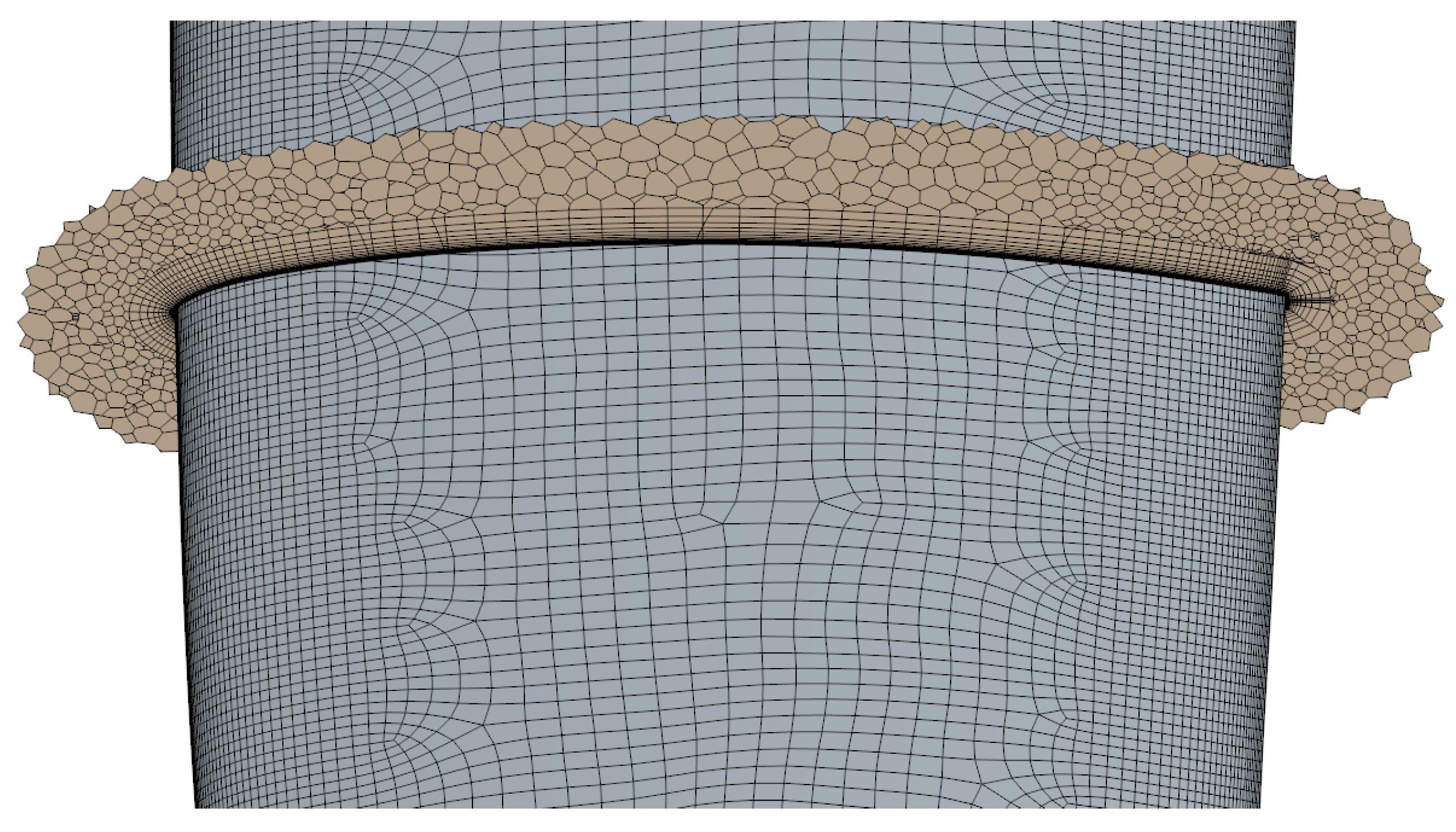
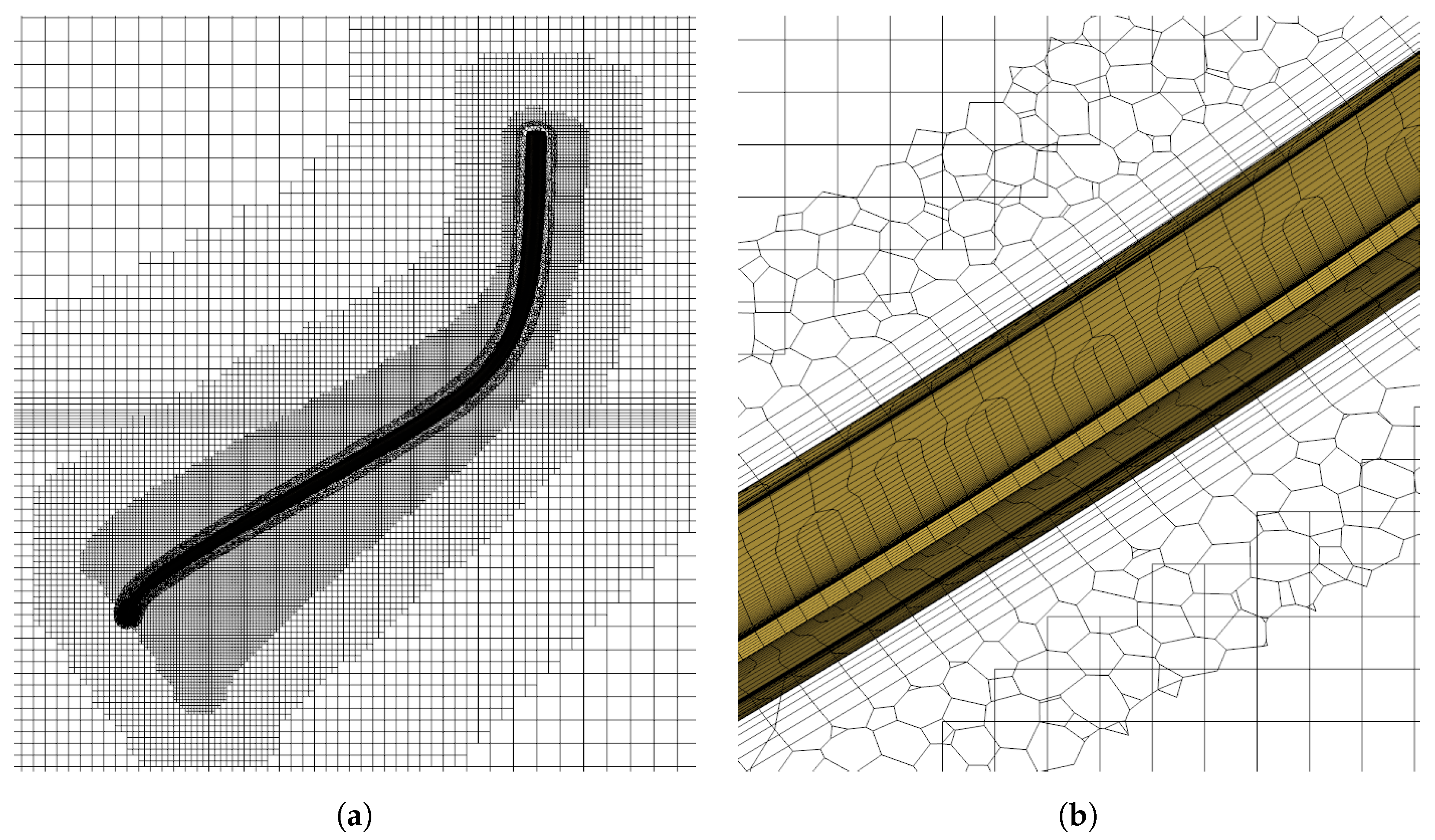
The foil forces are strongly dependent on mesh resolution close to the foil and therefore a semi-structured mesh approach is used on the foil. The surface is re-meshed with quad dominant pattern with anisotropic refinements on leading and trailing edges. This results in an almost structured mesh, good control of mesh resolution close to leading a trailing edges and high quality of the cells. The surface mesh is extruded with the advancing layer method to create prismatic layers of cells to accurately resolve the gradients in the boundary layer. Figure 7 shows the surface mesh on a part of the foil and a section cut of the mesh illustrating the prismatic layers of the mesh. The polyhedral meshing algorithm is used further from the wall. In the validation model the polyhedral mesh is used in the entire domain. In the other models where free surface is present, a trimmer meshing algorithm is used in the far-field to include anisotropic surface refinement for the free surface resolution. The polyhedral mesh is in those cases constrained to a small domain 30 mm from foil surface. The two meshes are combined with an overset mesh approach. Figure 8a shows the mesh in a vertical cross section around the foil and Figure 8b shows a zoom of the section close to the foil. The most important mesh settings are listed in Table 3. In cases with waves the free surface refinement is expanded to cover the wave elevation and the waves are resolved with a minimum of 200 cells per wave length in horizontal direction and 20 cells per wave height in vertical direction. The rudders and elevators are meshed in the same way as the foils and contained in their own overset mesh and additional refinement are used on the background mesh to ensure equal cell sizes and proper resolution of water surface deformation as seen in Figure 9 that shows a horizontal cut through the mesh at the level of the water surface. The total number of FV cells used in the simulation models are listed in Table 2.

Figure 7.
FVM mesh on foil and a section showing the prismatic layers.

Figure 8.
FVM mesh for foil performance simulations: (a) cross section; (b) cross section zoom.
Table 3.
Mesh sizes for the fluid mesh.

Figure 9.
FVM mesh of case with both rudders and foil horizontal cut plane.
2.2.3. Flow Models and Solvers
A RANS model with k- SST [22] turbulence model is applied to model the flow. In the models with free surface both air and water are modelled with the Volume Of Fluid (VOF) method [23]. The modified High Resolution Interface Capturing (mHRIC) convection scheme [24,25] is used to keep the interface between air and water sharp. The modified scheme is used because it gives less numerical dissipation for wave propagation. Second order up-wind scheme is used for spacial discretisation. The flow is solved with a segregated solver with an Semi-Implicit Method for Pressure Linked Equations-Consistent (SIMPLEC) pressure velocity coupling algorithm with 2nd order backward difference implicit unsteady time integration [26]. To investigate transition the two equation correlation based - transition model [24,27] is applied with a correlation model from Abu-Ghannam and Shaw [28]. Waves are modelled as 5th order waves and applied as pressure and velocities at the boundaries of the domain. The setup for wave simulations is based on Refs. [29,30]. No wave forcing is used. In the cases where the boat is free to heave and/or pitch the boat motions are solved with the build in 6-DOF motion solver. The moment of inertia is based on a complete CAD model of the boat, mast, and sails and the values are listed in Table 4. The time step required for the unsteady foil simulation is found to be less than 50 ms according to [14] and for the dynamic simulations a time step corresponding to 250 steps per wave period or period of forced oscillation is needed. In the FSI case the time step is dictated by the stability of the coupling.
Table 4.
Mass moment of inertia of the boat.
2.3. Fluid Structure Interaction
The solid and fluid flow models are solved separately, but the coupling is implicit and information is exchanged between the solvers at every inner iteration of the time step. Information is interchanged at the interface corresponding to the foil surface, the surface highlighted in yellow in Figure 1. Pressure and shear stresses are transferred from the flow model to the solid model and deformation is transferred the other way. Since the mesh of the two models are non-conformal the values must be interpolated at the interface. The interpolation is based on the 2nd order FEM shape functions. The fluid mesh is deformed to match the deformation of the solid using B-spline interpolation [24].
Fsi Stabilization
Without stabilization the model can become unstable. Two methods of stabilization are used in the present work. For steady state simulations an under-relaxation is applied to the deformations. A constant displacement under-relaxation factor of 0.1 is used corresponding to 10% of the predicted displacement is applied at a given iteration. This method gives no loss of accuracy since the resulting solution is a steady state and the under-relaxation only delays convergence. In the unsteady cases added mass is used to stabilize the structural model. A custom added mass equivalent to of water is used at the FSI interface. This corresponds to that the foil is moving the surrounding water a chord length from the foil surface. The initial added mass estimates are based on forced oscillation simulations presented in [14]. Different values of the added mass from 0.1 to 10 is tested, and are found to not affect results, but a minimum added mass of 0.2 is required to maintain stability. The added mass is the around the same size as mass of the foil. For more details on added mass on the foil see [14]. The stabilizing added mass is applied as a precondition for the implicit algorithm to stabilize the solid solver and has no impact on the accuracy of the solution. To test that the added mass stabilisation does not influence results, simulations are run with varying added mass, and no changes in results is observed. The actual added mass effect is inherently included in the strong solver coupling. The number of iterations required to convergence within each time step depends on the changes in the present time step and this is controlled by the level of the solid model residuals. A maximum of 15 and a minimum of 5 inner iterations is used. 5 iterations are required for the fluid flow solver to converge. The coupling is found to be stable for time steps up to 5 ms and all simulation models without periodic motions are using this time step. In the cases with waves or motion the time step is set to ensure 250 time steps per wave period or period of forced oscillation.
2.4. Experiments
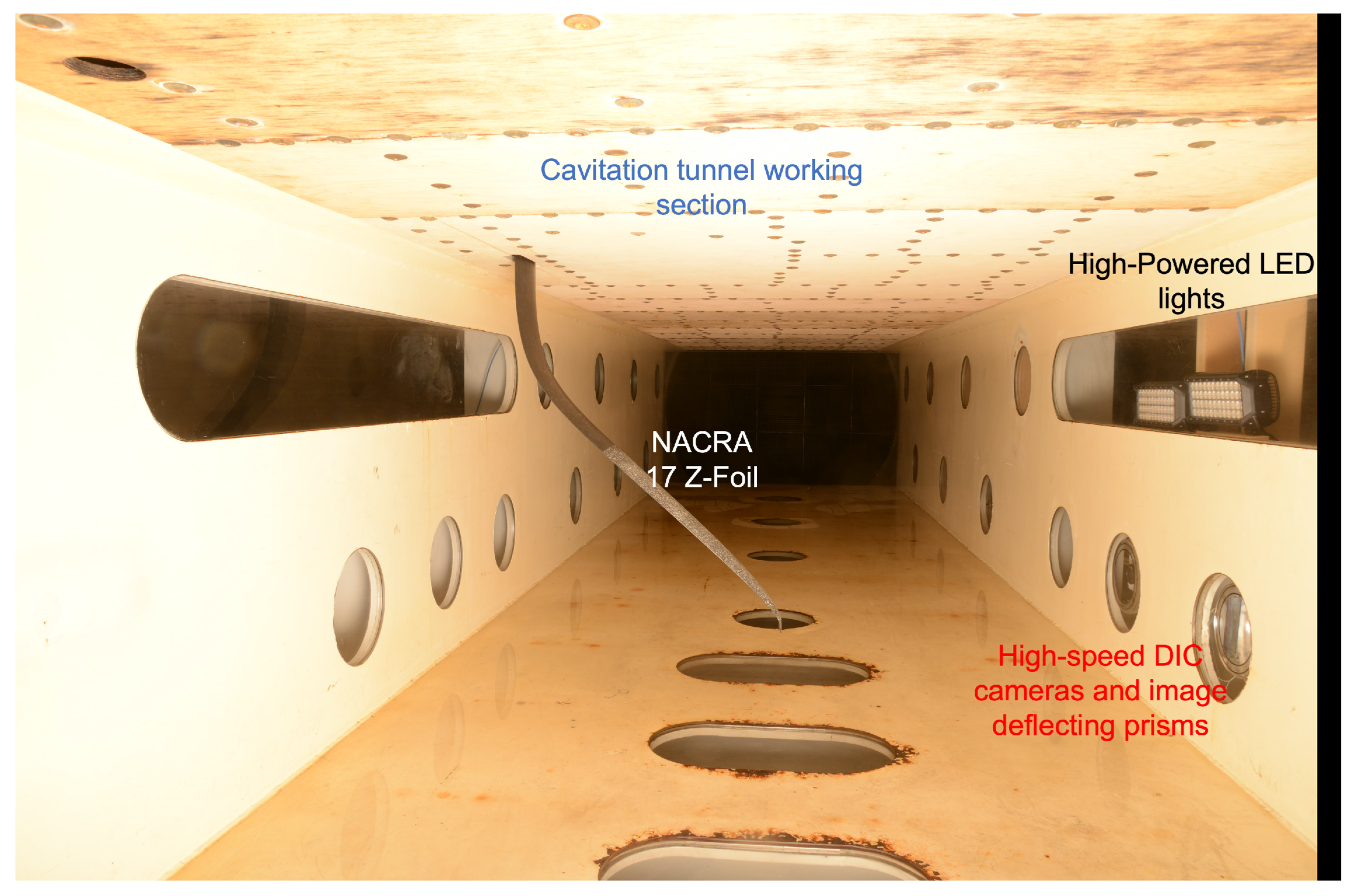
The numerical FSI model is validated by comparing with experiments conducted in the cavitation tunnel at RISE SSPA maritime center. In the experiments the foil is mounted in the cavitation tunnel in a similar way as in the boat as shown in Figure 10 and exposed to a water flow of up to 9 m/s. Forces and moment are measured with a six-component force balance and deflections are measured with a stereo Digital Image Correlation (DIC) system. The foil is tested in a large range of conditions with varying flow speed, leeway angle and rake angle. The experiments are described in further details in [8].

Figure 10.
Cavitation tunnel test section with foil as presented in [8].
In addition to the FSI experiments performed in the cavitation tunnel a structural test of the NACRA 17 foils has been performed at RISE SSPA Maritime. The foil is mounted in a rigid frame exactly replicating the mounting on the boat and the foil is loaded with a known weight. Deflection of the foil is measured by visual tracking using Qualisys system with 4 Motion capture cameras series 7+ applying tracking markers at different locations on the foil. The foil is loaded at locations close to the leading and training edges and the resulting deflection is tracked with the markers at both loading locations. The structural test, shown in Figure 11, was performed on 32 z-foils and it gives an indication of the bending and torsional stiffness of the foil. The averaged values of bending and torsional stiffness among the 32 tested is used for the reconstruction of the structural properties of the foil. The maximum static load applied to the foil is 70 kg, and the foil is pre-loaded to minimise uncertainty in the zero-load condition.

Figure 11.
Rig used to test the structural twist and deformation of a NACRA 17 foil.
2.5. Validation and Uncertainty
To validate the numerical FSI model the uncertainties of both numerical model and experiments must be estimated. The approach adopted is the one from [31], where more details of the approach can be found. The main uncertainty of the numerical model is the discretisation uncertainty. To estimate this, multiple simulations with varying mesh sizes are run and a power law is fitted to the resulting forces and displacements using a least squares approach.
where is the fitted quantity, h is a characteristic cell size, is the estimated quantity at zero cell size, and c and p are fitting coefficients. Ideally p should be 2 for 2nd order spatial discretisation. The power law is used to estimate the discretisation uncertainty together with the standard deviation of the fit and a safety factor. The discretisation uncertainty is estimated at a single point and the estimate is re-used for all compared cases. Another important uncertainty is the uncertainty of the material properties of the foil structure. Since the model is fitted to an average value from the structural test the uncertainty is estimated based on the standard deviation of the structural tests. This uncertainty is added as an input uncertainty for the numerical model. The convergence uncertainty is found by letting the solver run another 1000 iteration and comparing to the solution where it is normally stopped.
The highest uncertainty of the experiment is the alignment uncertainty in the leeway direction. The service technicians in the test facilities have estimated the alignment uncertainty to be 0.5°. The corresponding uncertainty on the displacement and forces are estimated based on the experimental data at 0.5° from the validation point. The repeatability uncertainty is based on the double point in the experimental data and uncertainty on the velocity in the cavitation tunnel is based on the uncertainty of the pressure sensors used to calculate the velocity.
Forces are extracted from the simulation and presented in non-dimensional form
where i is the force direction, is the force, A is area, is water density, and V is flow velocity. The area used is the wetted area at zero rake and respective flying height. Displacement is reported as the maximum displacement.
2.6. Performance Test Matrix
To investigate foil performance a test matrix, shown in Table 5 with variations in flying height, rake and leeway angles is investigated.
Table 5.
Test matrix used for performance evaluation.
The test matrix is evaluated for 18 knots of boat speed both with and without FSI for comparison. In addition, a number of cases is run with flying height 0.6 m and leeway 2°.
2.7. Environmental Conditions
The fluid properties used for the simulations are based on the ITTC guidelines [32] and listed in Table 6. For the validation study the temperature in the cavitation tunnel is used and for the open water simulations conditions are based on the weather in Marseilles at the beginning of August, when the Olympic games will take place. The waves used are based on data collected from a wave buoy located in the bay of Marseilles on the 7th of August 2023 [33]. The data is for a specific day with mistral conditions cf. Table 7. The wave high from the observations was 1.06 m. This wave height gave physical instabilities for the model without the presence of crew adjustments. Instead a reduced wave height of 0.5 m is utilized for the simulations. Waves and wind are assumed to be from the same direction. Based on observations from the boats during racing the foil and rudder settings and the platform pitch of the boat in this condition is estimated and listed in Table 8.
Table 6.
Fluid properties used in simulations.
Table 7.
Weather data used in simulations. TWS is True Wind Speed, TWD is True Wind Direction, T is wave period and H is wave height.
Table 8.
Boat parameters for simulation of boat sailing upwind in Mistral condition.
3. Results
3.1. Validation and Verification
In this section efforts to verify and validate the numerical FSI model are described. Discretisation uncertainties are evaluated separately for the solid and fluid flow models and the combined FSI model is validated against experimental data.
3.1.1. Solid Model Verification
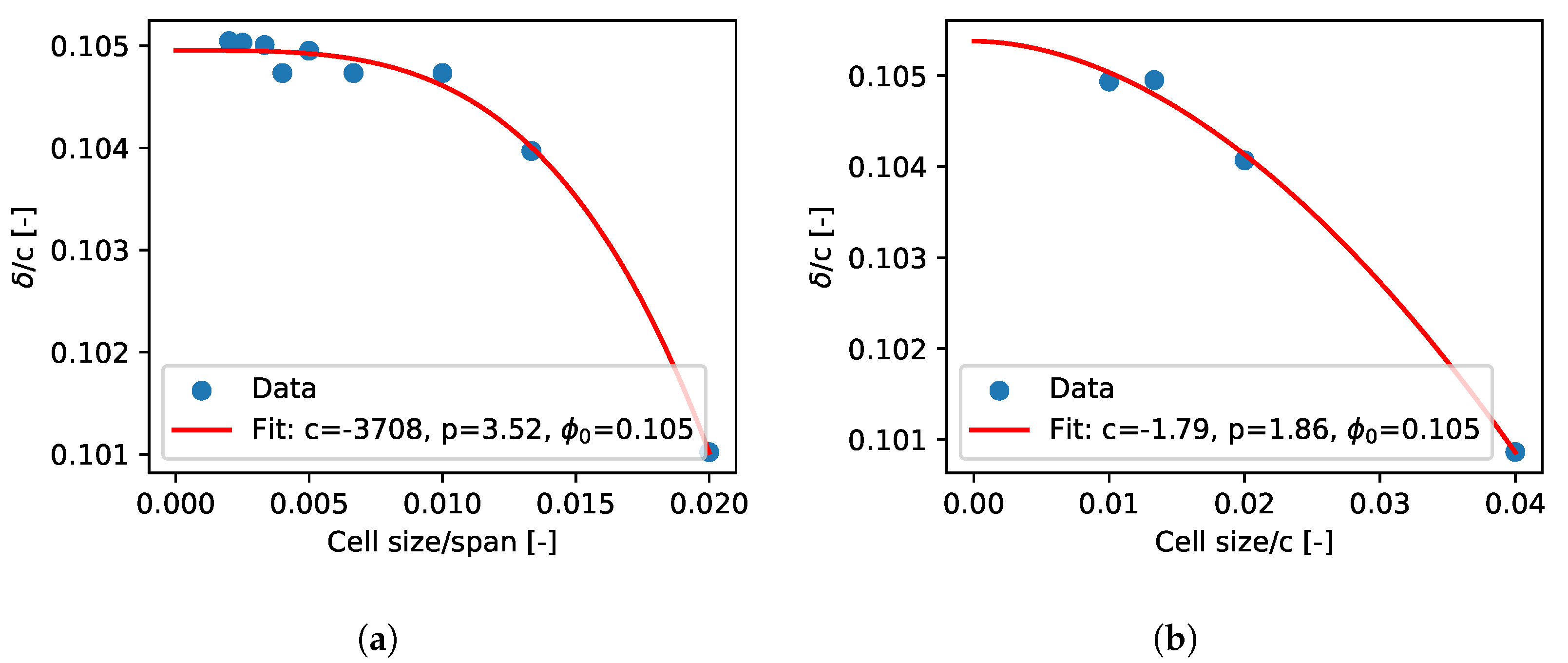
The structural model is verified by a detailed mesh convergence study and the material properties are fitted to match the average deflections found from structural tests of the foils. The structural foil test is replicated with the numerical model and the mesh size is varied in span and chord-wise directions separately. The resulting relative displacement are plotted in Figure 12 along with a power fit used to estimate the uncertainty. To secure a good mapping between solid and fluid model a relative mesh size corresponding to 200 cells in the span and 75 cell in the chord-wise direction is needed. The resulting discretisation uncertainties with this mesh based on the power fit and a safety factor of 1.25 is listed in Table 9. The cell size in the thickness of the shell is also investigated and it is found that a single cell in the thickness was sufficient to represent the displacement (not shown). For accurate representation of stresses more cells would normally be needed, but in this study only displacements are of interest. An average deflection from the structural tests of the 32 foils is used to find the material properties of the foil in the simulation. The Young’s modulus is adjusted until deflections are matched, while other properties are kept constant. The twist measured is used in an attempt to match anisotropic material properties of the foil, but the relative uncertainty of the twist is found to be too large to estimate the anisotropic behaviour. The measured twist is only 0.37° and the twist obtained with isotropic material properties is 0.31°. Therefore, isotropic material properties are used as listed in Table 1.

Figure 12.
Mesh convergence. Displacement over chord c as a function of relative cell size including power curve fitting for uncertainty estimation. (a) span-wise resolution; (b) chord-wise resolution.
Table 9.
Discretisation uncertainties for solid model for span-wise resolution (), chord-wise resolution (), and total ().
3.1.2. Fluid Flow Model Verification
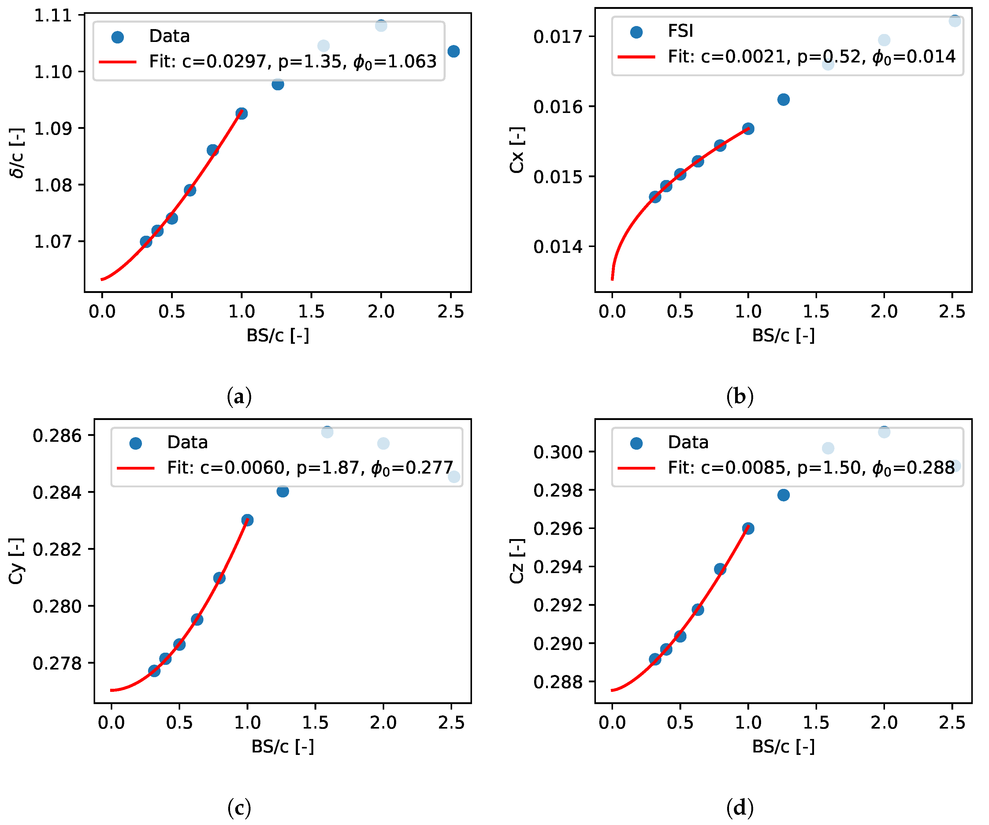
To verify the flow model a mesh convergence study is conducted for single velocity (7 m/s), rake angle (2°), and leeway angle (0°). The mesh size is varied by changing the base size with a factor of between each point. In total 9 meshes are investigated, with the finest mesh being 8 times finer than the coarsest. Table 10 lists the relative base size () and cell count of the meshes. All mesh controls depend linearly on the base size except the control for the prismatic cells. The prismatic cells are instead kept constant to ensure a wall y+ less that 1. Previous study has shown that a wall y+ of less than 1 is needed to ensure accurate prediction of the foil forces [14]. The resulting displacement and force coefficients are shown in Figure 13. To estimate the discretisation error a power law is fitted to the finest meshes using least squares. The coarse meshes are omitted from the fit as these are considered to be in the stochastic range, while the used meshes are considered to be in the asymptotic range. The approach used is similar to the approach found in [31]. A BS equal the chord length, BS/c = 1, is selected for the following work to keep computational expense at a reasonable level. The computational time is 500 CPU seconds per iteration. 1000 iterations are needed to reach convergence in these steady state simulation resulting in a total computational time of 144 CPU hours. In comparison the finest mesh in the study gives a computational time of 1600 CPU seconds per iteration, and this is unfeasible for transient simulation with several thousand iterations. Displacement is found to converge with an estimated uncertainty of 3.8% for a base size of 0.2 m cf. Table 11. The drag force does, on the other hand, not show a converging trend for the investigated range of mesh sizes. The discretisation uncertainty of the drag is instead estimated from the finest mesh and with an increased safety factor of 1.5 this gives an uncertainty of 16.5%.
Table 10.
Meshes used for the verification of the fluid model. BS denotes the mesh base size and c the chord length.

Figure 13.
Mesh convergence. Forces and displacement as a function of base size (BS) over chord (c) including power curve fitting for uncertainty estimation. (a) displacement over chord c; (b) drag force coefficient ; (c) side force coefficient ; (d) lift force coefficient .
Table 11.
Discretisation uncertainties. is the difference between the value at the applied mesh size and the asymptotic value, is standard deviation of the fit and S is the safety factor.
3.1.3. Fluid Structure Interaction Model Validation
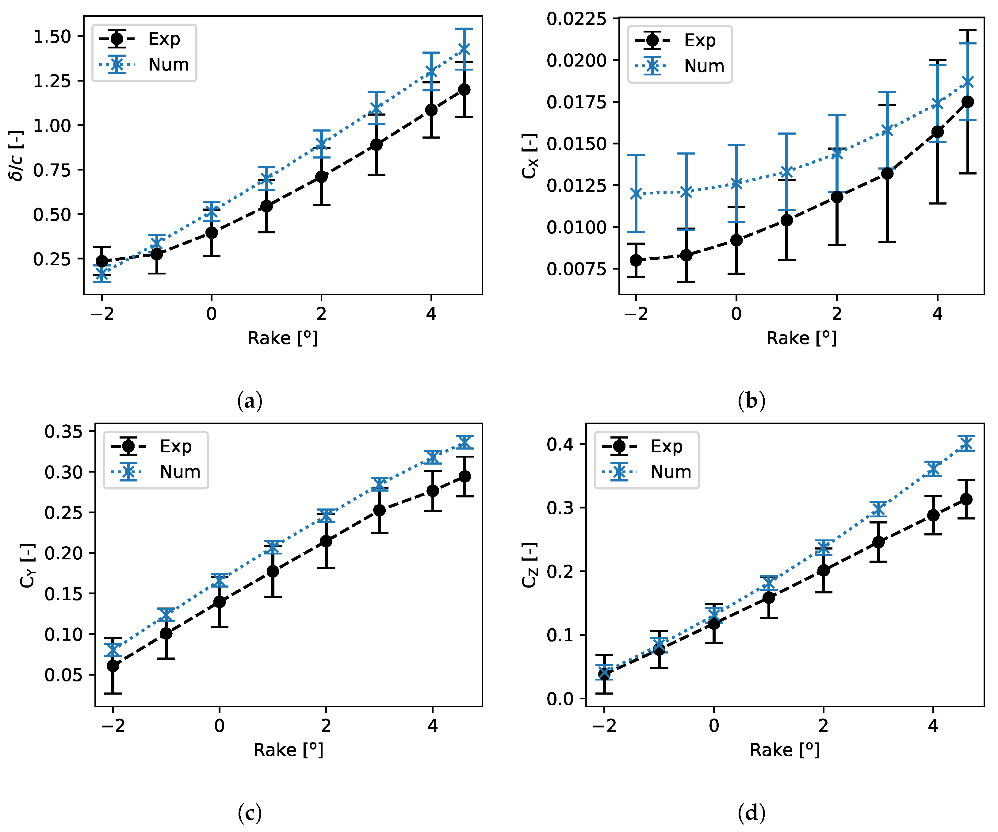
The numerical FSI model is validated against the experiments performed in a cavitation tunnel. There is a large number of experiments that could be used for comparison, but for simplicity a single speed and leeway angle are chosen. Additional experimental values can be found in [8]. Thus, a speed of 7 m/s is used because it has the most complete test matrix. The leeway angle used for comparison is 0°. Figure 14 shows the comparison of numerical and experimental results for displacement and force coefficients for the range of rake angles investigated. Error bars indicate the uncertainties. The uncertainties and the differences between the experiments and the numerical models are shown in Table 12, Table 13, Table 14 and Table 15. The model is considered validated for the specific rake angle with the validation uncertainty listed if the difference between experimental and numerical model is less than the validation uncertainty. The full version of the validation tables including all uncertainties are listed in Appendixes Appendix A.1, Appendix A.2, Appendix A.3, Appendix A.4. There is a high uncertainty and the numerical FSI model tend to overestimate both forces and displacement. From the discretisation study (Section 3.1.2) it is clear that a finer mesh would reduce the forces and bring the results closer to the experiments and reduce uncertainty. The validation is performed with a mesh with a base size of 0.2 m and a finer mesh would make simulations excessively expensive.

Figure 14.
Numerical and experimental values as a function of rake angle with a constant leeway of 0°. Error bars indicate uncertainties. (a) displacement over chord c; (b) drag force coefficient ; (c) side force coefficient ; (d) lift force coefficient .
Table 12.
Validation summary for displacement . U is uncertainty, subscripts and denote experimental and numerical, respectively.
Table 13.
Validation summary for drag force . U is uncertainty, subscripts and denote experimental and numerical, respectively.
Table 14.
Validation summary for side force . U is uncertainty, subscripts and denote experimental and numerical, respectively.
Table 15.
Validation summary for lift force . U is uncertainty, subscripts and denote experimental and numerical, respectively.
There are some significant uncertainties associated with the validation. The alignment in the experiment is the most important, but uncertainties related to the geometry and stiffness of the foil are also significant. Although not quantified in this validation there is an uncertainty in the actual shape of the foil. The stiffness of the foils is found to vary and the simplified internal geometry of the foil and material properties used in the present study might give rise to higher uncertainties. Another aspect is transition. As investigated in Section 3.2.2 transition as a profound effect on forces and modelling of transition might change the outcome of validation. Transition is, however, significantly affected by the turbulence intensity and this is unknown in the validation tunnel experiment. Measurements of turbulence intensity and modelling of transition could improve validation.
Validation is performed in steady state and remaining simulations are unsteady due to the presence of the water surface. To ensure the simulations are compatible the validation model is run with the unsteady solver at a rake angle of 2 ° and compared. The displacement and forces are found to within 0.1% of the steady state simulations.
3.2. Foil Performance
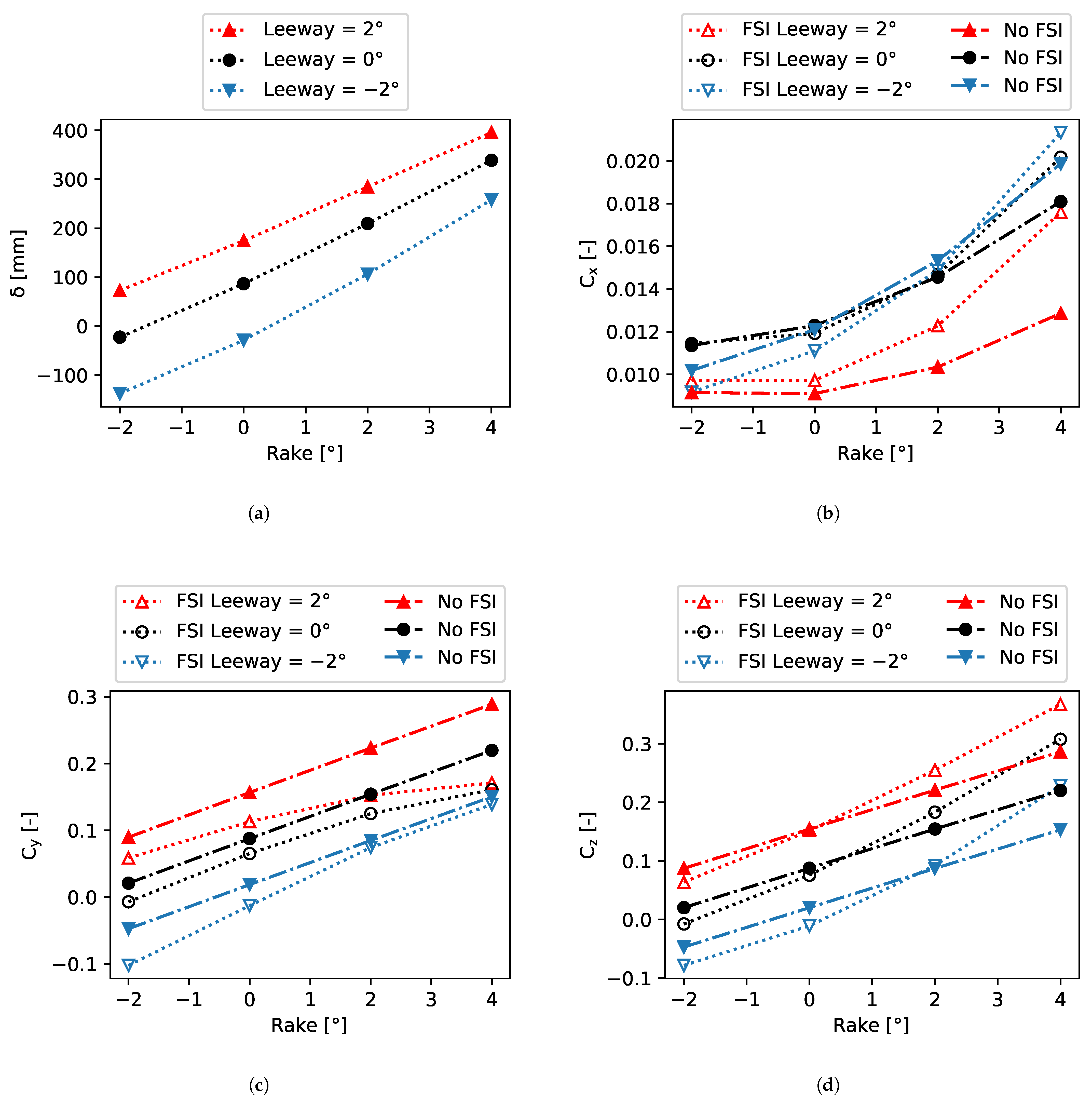
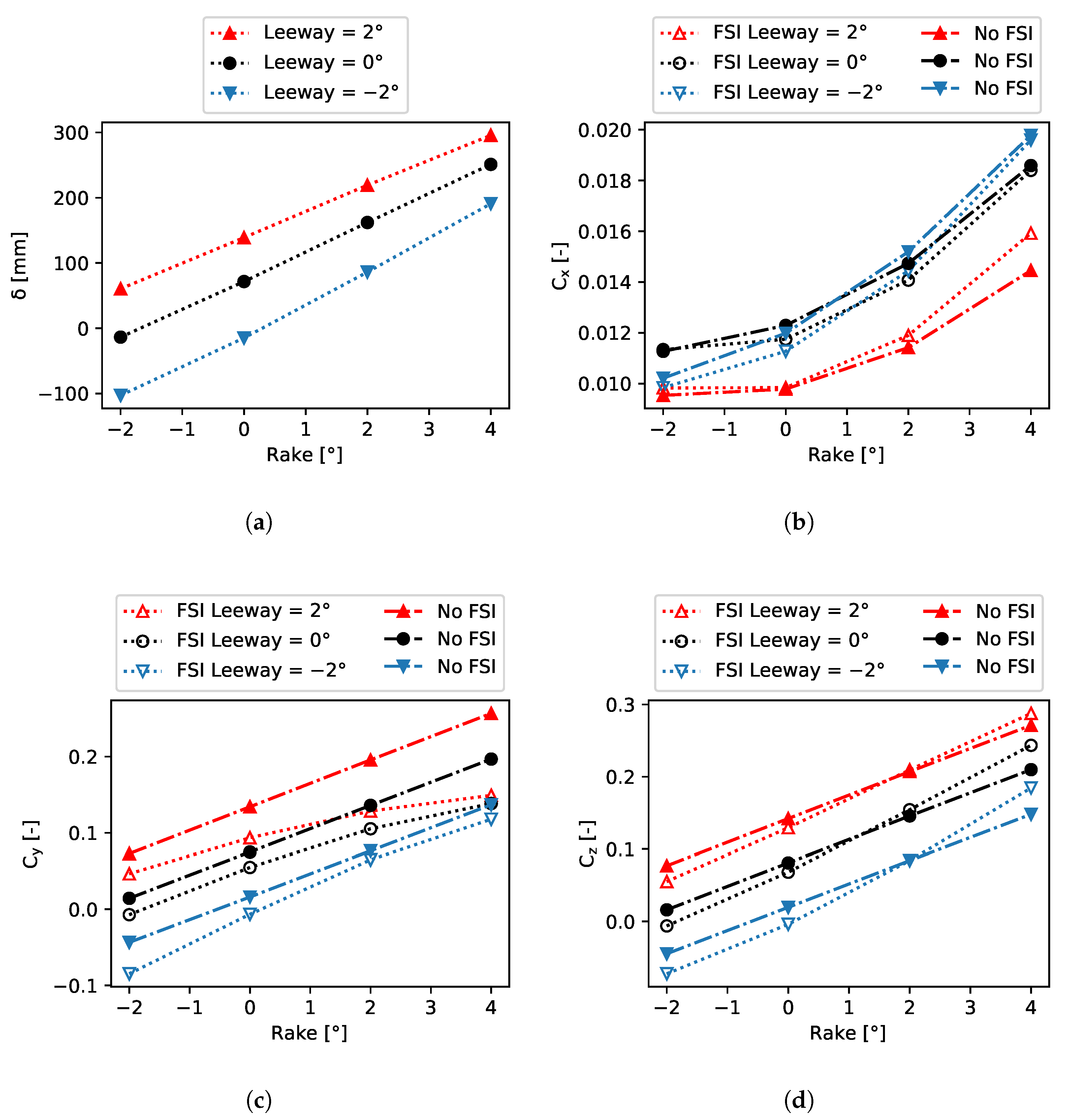
To evaluate the foil performance over a wide range of conditions simulations are conducted at all point of the simulation matrix shown in Table 5 both with and without FSI. Figure 15 shows the results for a flying height of 0.6 m. Results for the other two flying height are in Appendixes Appendix B.1 and Appendix B.2. The displacement shown in Figure 15a increase linear with rake angle and leeway angle. The maximum displacement is 300 mm corresponding to 1.5 times the chord length. The effect of displacement is assessed by comparing the simulations with and without displacement. The side force coefficient in Figure 15c is decreasing with increasing deflection. This is expected since the deflection will reduce projected area in the side force direction and thereby the force. The coefficients are normalized with a constant area for each flying height. The vertical lift force coefficient is increased with deflection as seen in Figure 15d, but the increase is smaller than the decrease in side force indicating an effect of twist of the foil. Twist during deformation can reduce the angle of attack and thereby the total lift force. The drag force shown in Figure 15b appears to be less sensitive to deflection and increase in some cases while decreasing in others. The deflection and forces at the other two investigated flying height show the same trends.

Figure 15.
Foil performance simulation results for 0.6 m flying height. (a) displacement ; (b) drag force coefficient ; (c) side force coefficient ; (d) lift force coefficient .
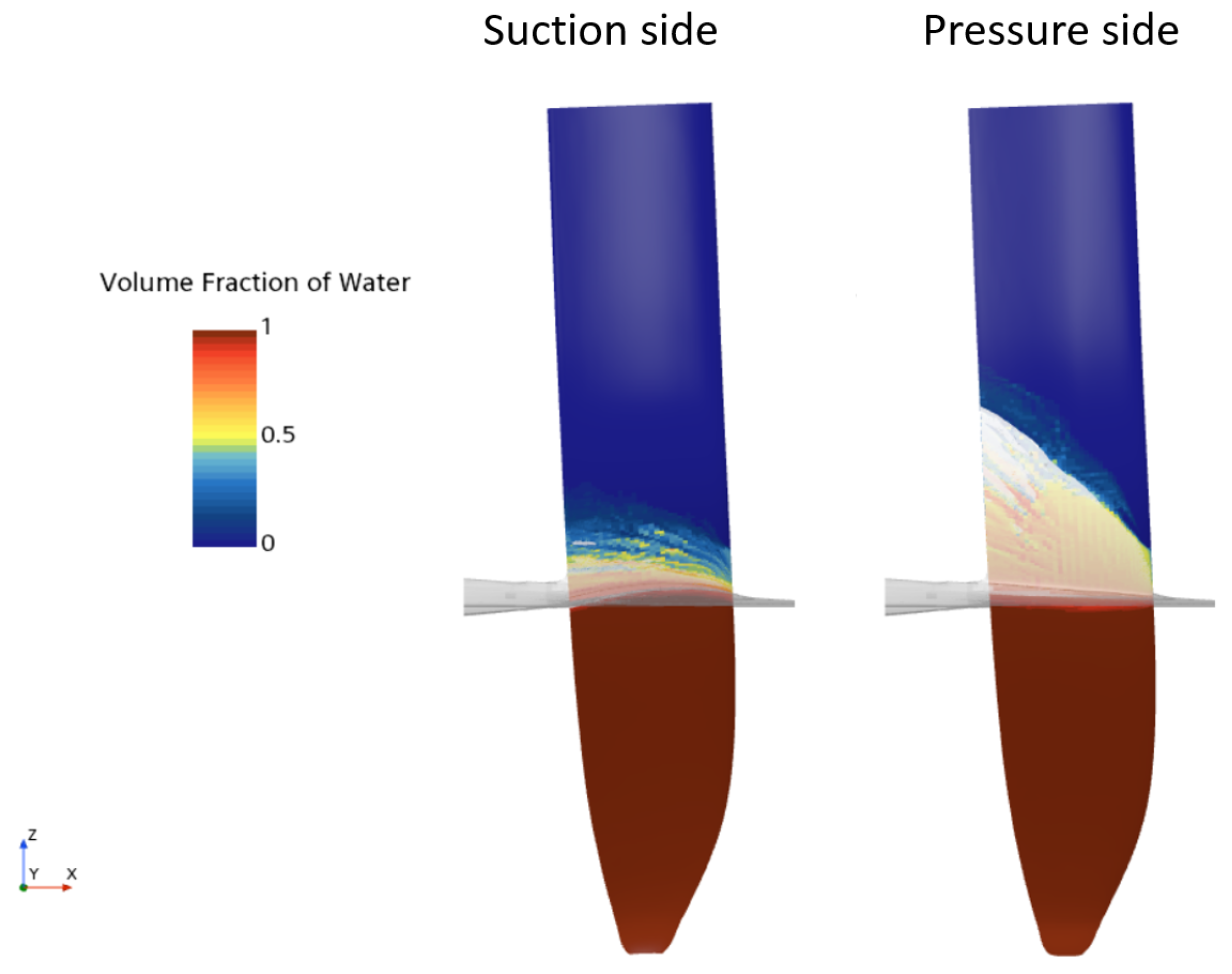
Surface piercing hydrofoils are known to be prone to ventilation [34,35]. To check for ventilation on the foil surface the volume fraction of water is plotted on the foil surface for a highly loaded case in Figure 16. The water sprays up, but there is no sign of air being pulled down on the suction side. No ventilation is observed for any of the investigated foil settings. This confirms what has been found in previous study [36], that ventilation only happen for extreme loading.

Figure 16.
Side view of the volume fraction of water on the surface of the foils for case with Flying height 0.6 m, Leeway 2° and rake 2°. The free surface is included as a transparent surface. Flow from right to left.
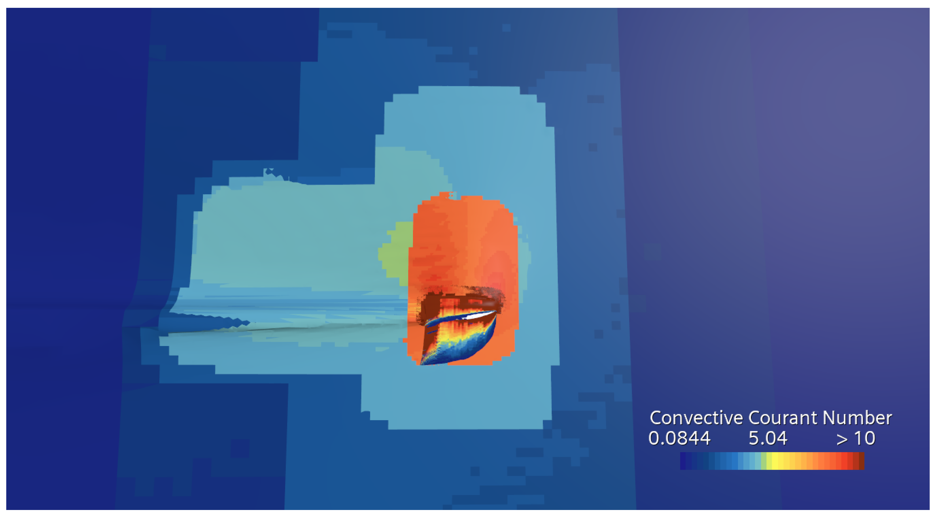
In Figure 17 the convective Courant number is plotted on the free surface for the maximum time step of 5 ms. The convective Courant number is higher than 1 and in some areas higher than 10. The solution remains stable due to implicit nature of the time integration and that the final flow solution is steady. Moreover, no smearing of the free surface is observed and forces and deflections changes less than 0.1% if time step is reduce an order of magnitude (now shown). In the cases where the solution is transient a lower time step is utilized to secure capturing of correct transients.

Figure 17.
The convective Courant number on the free surface for the case with flying height 0.6 m, leeway 2°, rake 2°, and a time step of 5 ms.
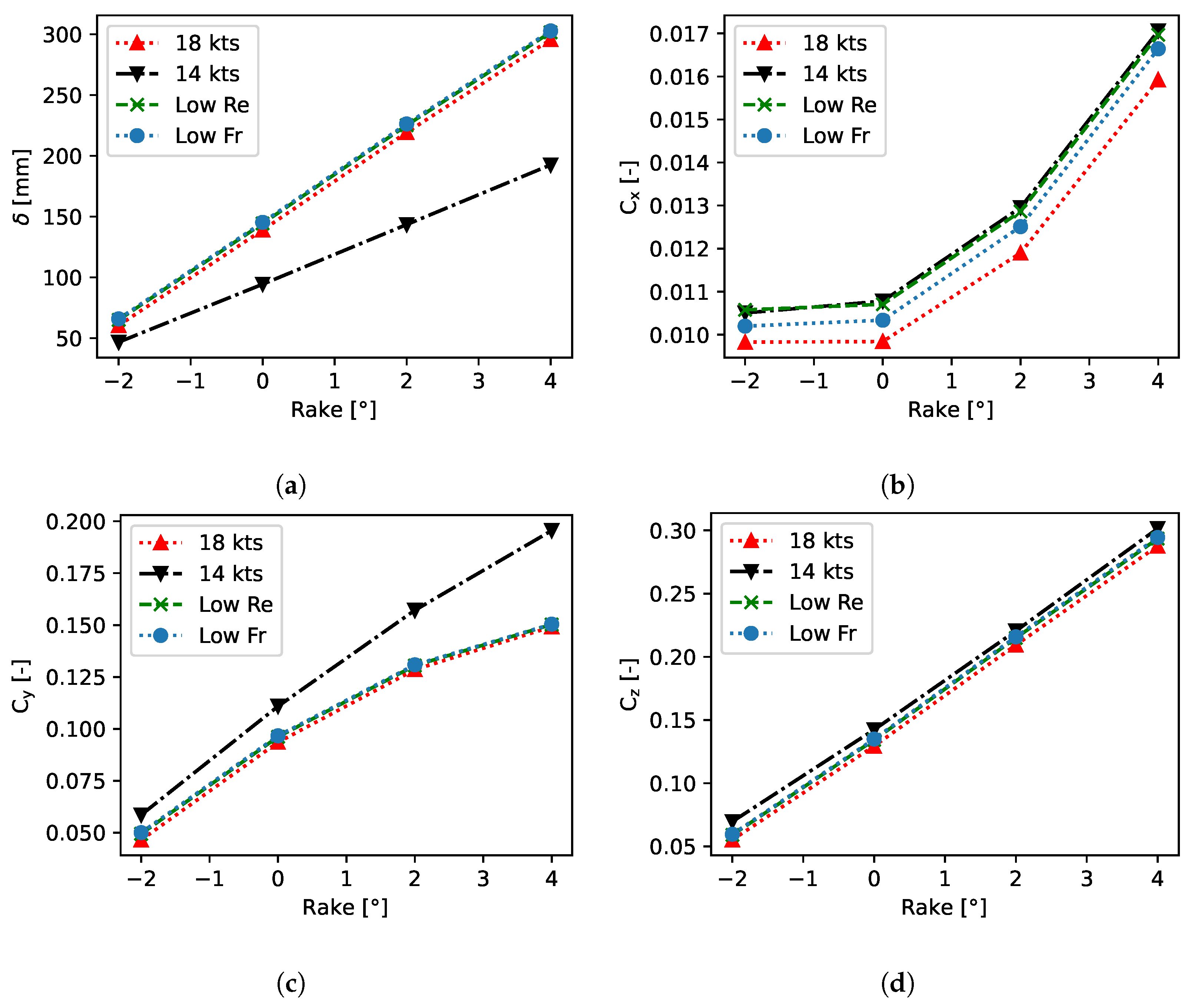
3.2.1. Effect of Speed
The foiling speed of the NACRA 17 ranges from 14 knots to more than 20 knots. This change in speed will affect the forces and deformation of the foils. To better understand the effect of the change in speed the change is made in three different ways. The first way is to simply change the speed from the previous used 18 knots to 14 knots. The second way is by only changing the Reynolds number to isolate this effect of change is viscous flow. The final way is to change only the Froude number to investigate the effect of changes in the free surface deformation. The Reynolds number is changed by changing the viscosity to match the Reynolds number of 14 knots, while the Froude number is changed by changing the gravitational constant. Flow parameters from these investigations are listed in Table 16. Only the flow properties of water are considered here.
Table 16.
Flow parameters of speed change study.
Simulations with the modified flow parameters are performed for a leeway angle of 2° and the full range of rake angles. The displacement shown in Figure 18a shows a large change in displacement due to change in speed, while the change in Reynolds and Froude number does not change the displacement significantly.

Figure 18.
Effect of speed change on foil performance for leeway 2°: (a) displacement ; (b) drag force coefficient ; (c) side force coefficient ; (d) lift force coefficient .
The drag coefficient is increased as the flow speed is reduced as seen in Figure 18b. The reduction in Reynolds number appear to resemble this effect closely indicating that the change is mainly related to the change in viscous drag forces due to change in Reynolds number. The reduction of Froude number also shows a change towards the reduced speed case indicating an effect of the wave making resistance. The side force coefficient shown in Figure 18c is also increased with the reduced flow speed, but in this case the change in Froude and Reynolds number does not account for any significant part of this increase. From the cases without FSI shown in Figure 15 it appears the deflection of the foil reduces the side force significantly. This effect is smaller in the case of smaller speed and smaller deflection. Thus, the increase in side force coefficient for the reduced speed is due to smaller deflection of the foil. The picture is less clear for the lift coefficient shown in Figure 18d. The lift coefficient is increased by reduction in speed, but in this case, it appears to be a combined effect of both Reynolds number, Froude number, and deflection. Another aspect is the twist of the foil during loading that can unload the foil due to reduction in angle of attack.
3.2.2. Effect of Transition
At 18 knots the Reynolds number based on the chord is 1.4 million and a transition is expected to happen somewhere along the chord. The position of this transition point can influence both the lift and drag of the foil and therefore the performance. To investigate the effect of transition, simulations of the foil with the - transition model is compared with fully turbulent simulations. To better predict the point of transition and thereby the forces the chord and span-wise mesh resolution on the foil is increased. The maximum cell size on the foil surface for transition simulation is 1.5% of chord which is half the size used in simulations in the other sections. To ensure an accurate comparison between the simulations with and without transition the simulation is rerun with this refined mesh for the comparison cases. Both cases are run without deformation to isolate the effect on the forces. Figure 19 shows the forces from the simulation with and without transition. The drag force in Figure 19a is reduced by 13% to 33% by including transition indicating a large part with laminar flow in the foil.

Figure 19.
Effect of transition on foil forces for leeway 2°: (a) displacement ; (b) drag force coefficient ; (c) side force coefficient .
This is confirmed by inspecting the wall shear stress in Figure 20.

Figure 20.
The wall shear stress on the foil (seen from above) with transition modeling illustrates the point of transition. Leeway 2° and rake 2°. Flow from right to left.
The abrupt change from blue (low wall shear stress) to red (high wall shear stress) indicates the transition position. The transition increases the side Figure 19b and lift Figure 19c force coefficients, with a value between 0.005 and 0.007. For the small rake angles this is a significant contribution of almost 9%, but for the larger rake angles the effect is only around 2%. The profound effect of transition on forces indicate a strong effect also in the validation case. To investigate this the validation case is repeated with transition model and agreement with drag is significantly improved, while all other forces and displacement are further from the experimental values (now shown). One of the issues with transition modelling in this case is that the turbulence intensity in the cavitation tunnel is unknown. The turbulence intensity in the flow is known to strongly affect transition [24].
3.2.3. Foil Performance in Motion
The boat often sails in waves or experiences large motions that leads to changing flow conditions on the foil. To investigate the dynamic forces and effects of FSI on the dynamic forces a study with sinusoidal motion in heave is performed with and without FSI. The foil is moved vertically ±100 mm so that the flying height is changes between 500 mm and 700 mm at a frequency (f) of 0.5 Hz, reduced speed () of 92.6. The resulting displacement and forces are shown in Figure 21. The maximum deflection of the foil is found when the foil is moving downwards while the minimum deflection is when the foil is moving upwards. This is reasonable since the changing motion creates a change in the effective angle of attack on the foil. The deflection is however not sinusoidal and this can be caused by two effects. There is an effect of the change in static forces due to the change in flying height and there is an effect of delayed response of the structure to the forces. In the case without FSI the side and lift forces are sinusoidal and closely follow the motion with a constant phase shift. The drag has a slightly different shape due to the non-linear drag to angle of attack behaviour. The inclusion of deformation reveals many interesting observations. The average side force is reduced as in the simulations without motion. The variation is almost sinusoidal but there is an additional phase shift of the force relative to the motion due to the deformation. The amplitude of the drag and side forces are significantly reduced with FSI, but the amplitude of the lift force is actually increased.

Figure 21.
Foil performance in heave motion; (a) displacement ; (b) drag force coefficient ; (c) side force coefficient ; (d) lift force coefficient .
3.3. Full Hydrodynamic Simulation
The foil performance evaluation is a good way to understand how the foils work and may serve as an input to the performance predictions. However, to get the understanding of the full hydrodynamic performance both foils and rudders must be included. In the following section both foils are included as flexible, and the rudders are included as stiff elements. In future studies the flexibility of the rudders could be included. Since the focus is on investigating the foiling condition, the influence of the hulls is small and therefore not included in the simulations. The hulls and crossbars are included in some of the pictures, but this is only visually.
3.3.1. Rudder Toe-Out Angle
The two rudders are mutually connected and controlled together, but it is still possible to adjust the relative angle between them. This angle is referred to as the toe-out angle. Since both rudders and foils are included, it is possible to investigate the influence of toe-out angle on the drag and side forces of the two rudders. It is necessary to include the foils in this analysis because the rudders work in the wake of the foils and the inflow angle and water surface elevation at the rudders is strongly influenced by the foils. This is apparent from Figure 22 that shows the free surface elevation seen from the front of the boat.

Figure 22.
Free surface deformation in the area between the foils and rudders.
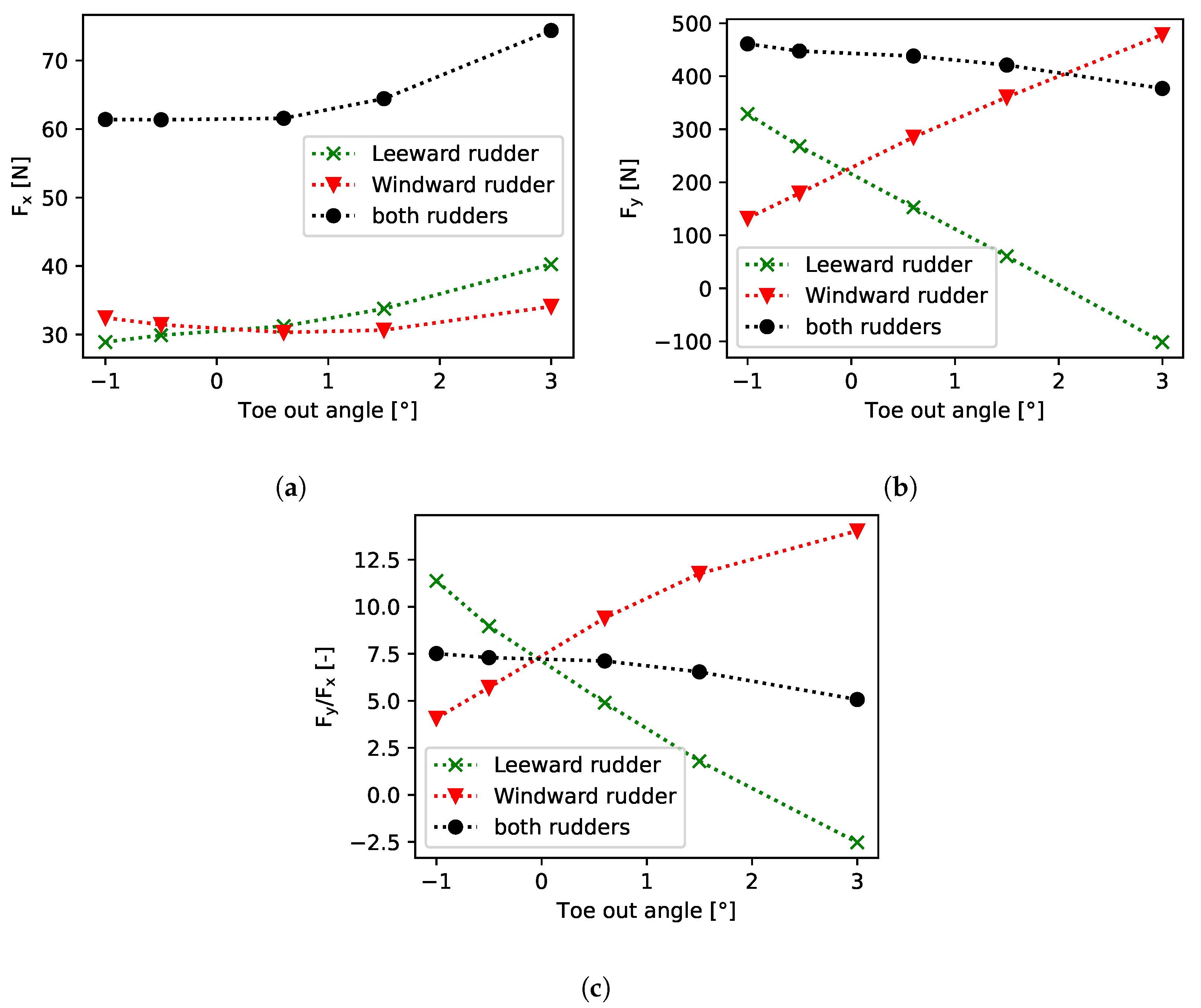
Five different toe-out angles have been investigated with a constant leeway angle of 2.5°. The resulting drag and side force production is shown in Figure 23a,b. The side force of the rudders change in opposite direction as the toe-out angle is increased as would be expected since one rudder will experience a reduction in angle of attack while the other will experience an increase. The combined side force tends to reduce with increasing toe-out angle. This effect can be attributed to the interaction with the wave system and the flow generated by the foils. The drag of the rudders tends to increase with toe-out angle indicating a change in induced drag due to the change in side force. The windward rudder has a small increase in drag for small negative toe-out angles apposed to the leeward that has a small decrease. This is not expected since the windward rudder should reduce the effective angle of attack while the leeward increases. The resulting drag is almost constant for toe-out angles between −1.0° and 0.5° but the side force are reduced with the increasing angle. As a result, the lift to drag ratio, shown in Figure 23c is largest for a negative toe-out angle.

Figure 23.
Rudder force with changing toe out angle of rudders: (a) drag force ; (b) side force ; (c) lift/drag .
3.3.2. Foiling in Waves
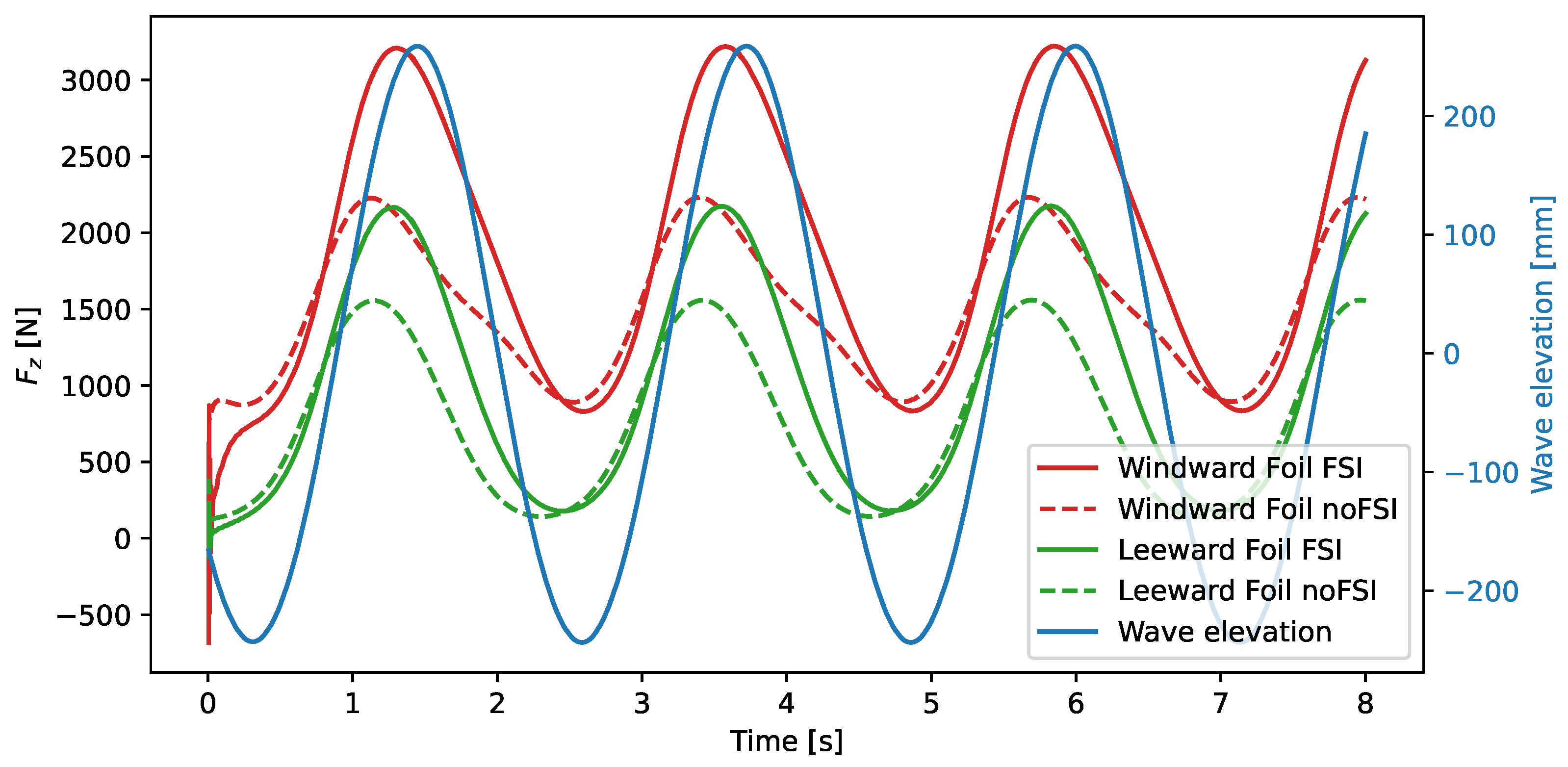
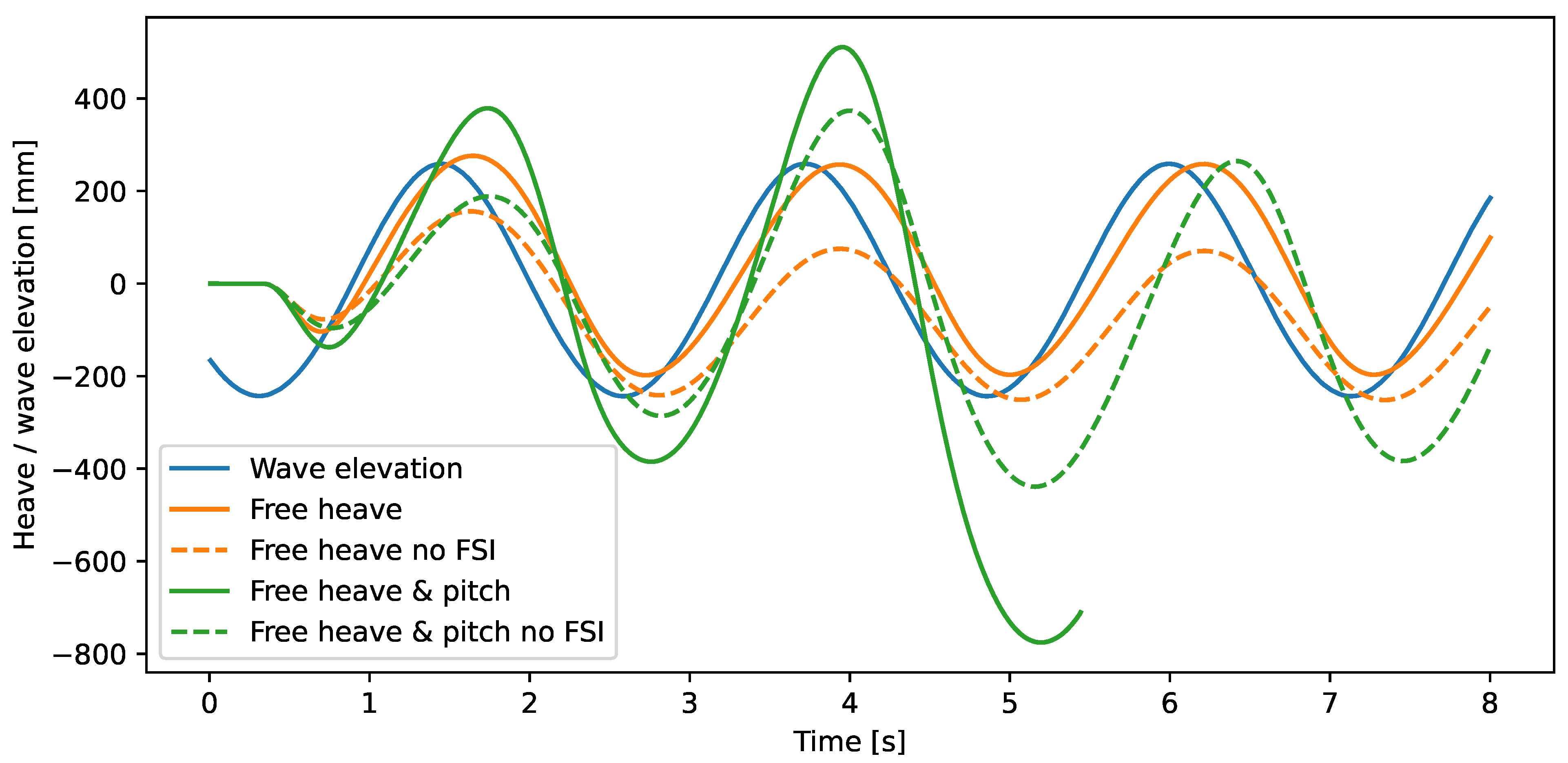
When exposed to waves the forces on the foils vary and so does the deflection and motion of the boat. A number of simulations have been conducted with varying degree of complexity. Firstly, the boat is exposed to waves, while fixed and without fluid structure interaction on the foils. Secondly, the flexibility of the foils is added. The resulting vertical lift forces on the two foils are shown in Figure 24 for these two cases together with the wave elevation. The leeward foil is carrying most of the load and deformation of the foils significantly increase the lift of the foils, especially the peak loads.

Figure 24.
Foil lift forces in waves.
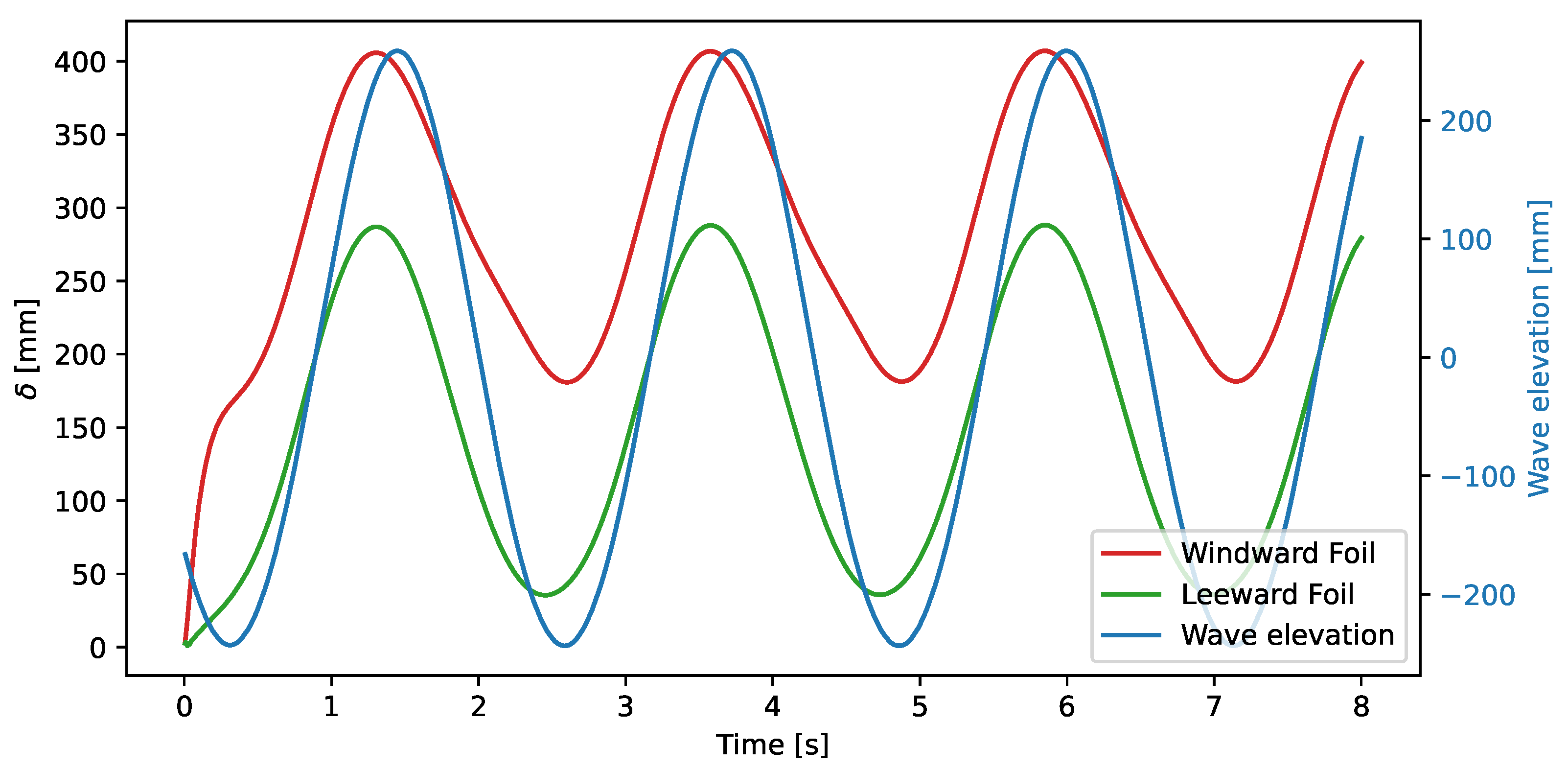
The displacement of the foils shown in Figure 25 follows the shape of the maximum lift and has attains a maximum of 407 mm.

Figure 25.
Foil displacement in waves.
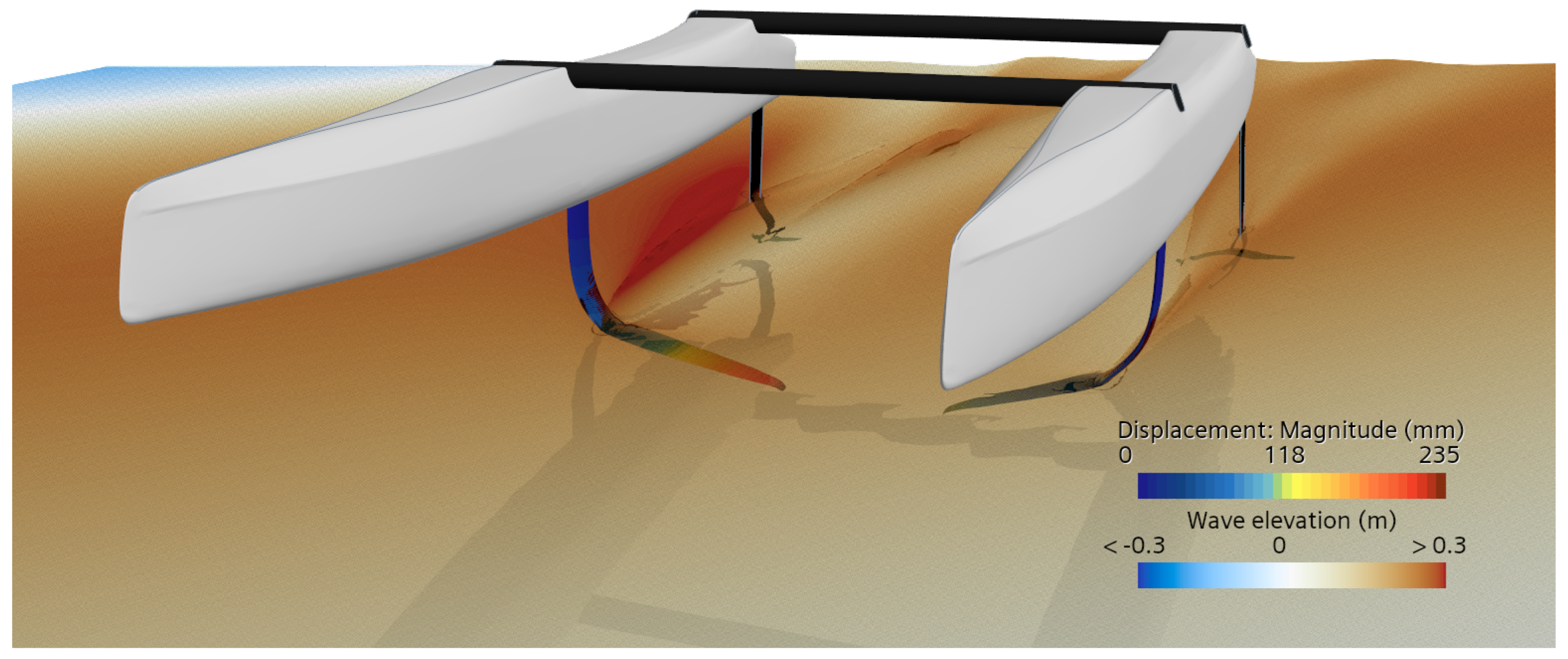
Next, the boat is set free to heave. A visualisation of the boat in waves with free heave and flexible foils is shown in Figure 26.

Figure 26.
Foil and rudder in waves with free heave motion.
In Figure 27 the heave motion of the two cases are shown as a function of time together with the wave elevation in the center of gravity of the boat. In the case with free heave and fixed pitch the motion follows the wave elevation with a small phase shift. The amplitude of the motion is 9% smaller than the amplitude of the wave. The motion is affected by the mass of the boat and the change in lift due to change in submergence.

Figure 27.
Heave motion in waves with and without free pitch.
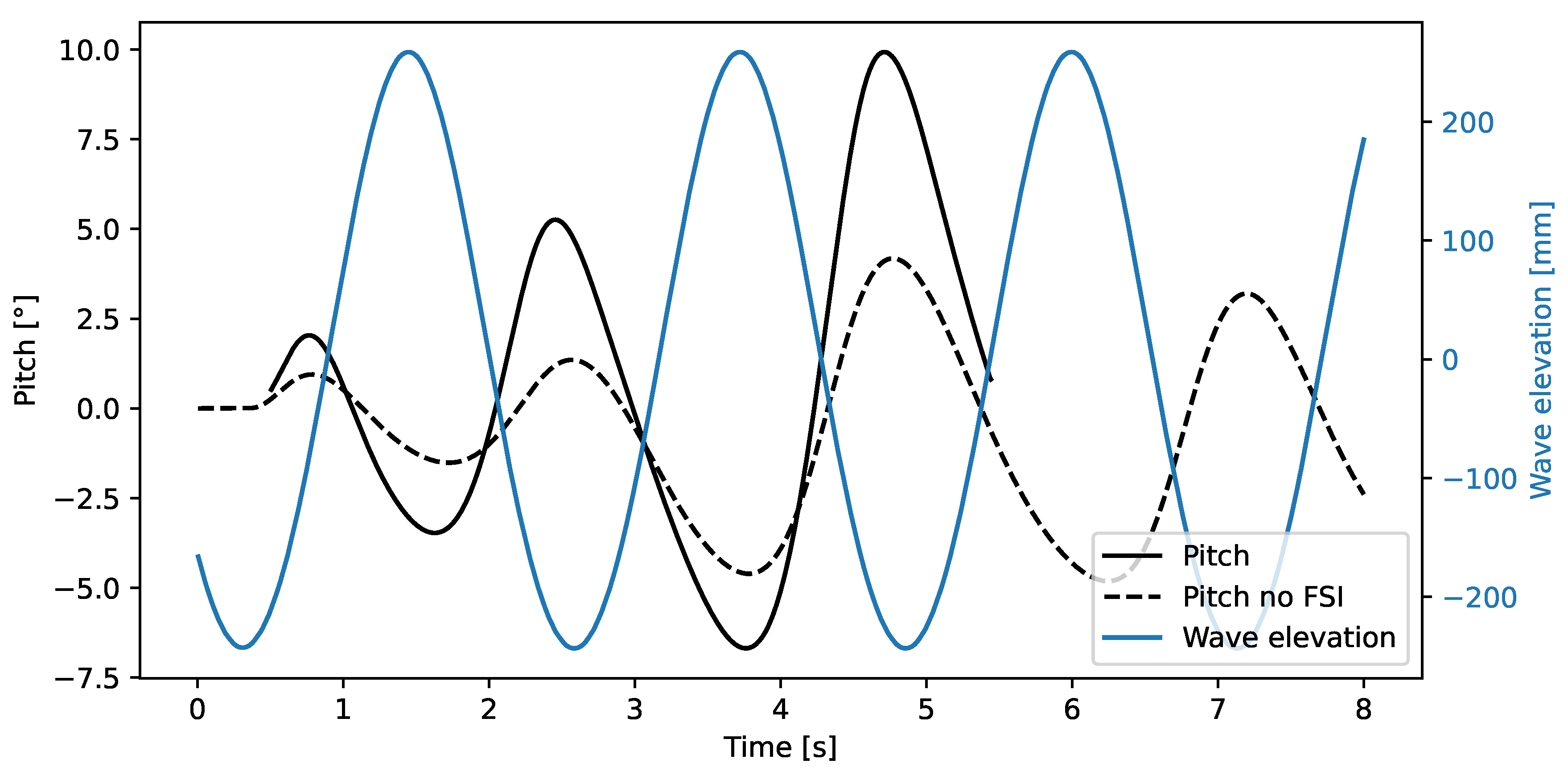
In the final case the boat is also released in pitch. The pitch motion is plotted in Figure 28 together with the wave elevation. The pitch motion is out of phase with the wave elevation and obtains high values after few seconds of simulation.

Figure 28.
Pitch motion in waves with free heave and pitch.
The large pitch variations also affect the heave motion as seen in Figure 27. The heave motion is increased to the point where it becomes too large and instabilities occur after 5.5 s simulation time. This result is well inline with reality since sailing in waves requires the sailors to constantly correct the pitch balance by moving their body weight forward and backwards in the boat. Without these adjustments the boat quickly gets out of control as in the simulation. In future works the motion of the sailors can be incorporated to control pitch motions in waves.
4. Conclusions
A numerical FSI model of the NACRA 17 z-foil has been developed. The model is based on a RANS FVM flow solution coupled strongly with a FEM solid model. The model is verified with mesh convergence studies of both flow and solid models and validated by comparison to experimental data. Structural properties of the model is found by tuning to structural test data and validation is performed by comparing to experiments of the foil exposed to flow in a cavitation tunnel. The model is in general found to over-predict drag force by 27%, lift forces by 17% and deflections by 17% compared to the experimental data. The validation is successful for some of the tested rake angles, but the validation uncertainty is high. Validation should be improved in future work by reducing some of the uncertainty. The most important uncertainties are foil internal structure and stiffness, foil alignment in cavitation tunnel, foil actual geometry, turbulence intensity and transition modelling.
Performance of the foil is computed for an extensive test matrix with variation in flying height, leeway angle, and rake angles both with and without deformation of the foil. The deformation of the foil affects the performance of the foil significantly. The side force is reduced and the vertical lift force is increased. Influence of transition is investigated by computing foil forces with an empirical transition model. Transition is found to reduce drag by 13% to 33% while increasing lift and side forces by 2% to 9%. The effect of speed on force coefficients are also investigated by changing Froude, Reynolds number, and flow speed in tree steps. The largest effect of speed is found in side force due to the change in deformation, while the drag force is changed due to the change in Reynolds number indicating that the effect is on the viscous boundary layer.
The foil is found not to ventilate in any of the tested steady state cases and this confirms findings from [36] that showed that the foil is only found to ventilate in extreme load cases. The risk of ventilation in dynamic cases is however not investigated, but should be investigated in future work.
The effect of foil deformation is even more important in case of motions. To test the effects of deformation in motion, the foil is moved in a sinusoidal heaving motion both with and without deformations. As in the steady case the average side force is reduced, and the amplitude of the side force is also reduced when deformation is included. Amplitude of drag is also reduced but the amplitude of lift is increased when deformation is included. This is an important result as increased flexibility will giver larger variation in vertical lift and thereby might affect stability during motion.
Both foils and rudders are included in a complete hydrodynamic model and the model is used to investigate the impact of rudder toe-out angle on drag and side forces on the rudders. Drag is found to increase with toe-out angle, but is almost constant between 1.0° and 0.5°. The side force reduces with toe-out angle, and this could indicate that small negative toe-out angle could be beneficial.
The full hydrodynamic model is also utilized to investigate sailing in waves. Simulations of the boat foiling in waves shows a significant impact of foil deflection on the resulting vertical lift forces. It increases when deformation is included. To see the effects on the boat motion the boat is set free first in heave and then in heave and pitch. The foil deflection is found to increase heave motion. This is inline with the finding for the prescribed motion case where vertical lift force is found to increase when foil deflection is included. In the case of free pitch the boat becomes unstable. This indicate that a stiffer foil might be beneficial when sailing in waves, however more investigations should be done to verify this at a wider range of conditions.
The developed FSI model is found to be stable and give valuable insights into foil performance and boat motions. The model has been verified and validated, but there is still high uncertainty. A more detailed investigation of foil internal structure and anisotropic properties could improve overall model accuracy. More investigations of the boat sailing in waves could help understand performances in dynamic conditions better. The movement of sailors could be included to ensure pitch stability of the boat.
Author Contributions
Conceptualization, All; methodology, All; software, S.S.K.; validation, L.M.G. and S.S.K.; writing—original draft preparation, S.S.K. and L.M.G.; writing—review and editing, All; visualization, S.S.K.; supervision, L.M.G., B.N.L. and J.H.W.; project administration, S.S.K. and J.H.W.; funding acquisition, J.H.W. All authors have read and agreed to the published version of the manuscript.
Funding
The numerical part of this research was funded by Team Danmark and the Novo Nordisk Foundation. The structural test rig is funded by the hydro- and aerodynamics Chalmers initiative and the cavitation tunnel tests by SSPA’s fond project.
Institutional Review Board Statement
Not applicable.
Informed Consent Statement
Not applicable.
Data Availability Statement
The data that support the findings of this study are available on request from the corresponding author.
Conflicts of Interest
The authors declare no conflict of interest.
Abbreviations
The following abbreviations are used in this manuscript:
| AWA | Apparent Wind Angle |
| AWS | Apparent Wind Speed |
| BS | Base size |
| CAD | Computer Aided Design |
| CFD | Computation Fluid Dynamics |
| DIC | Digital Image Correlation |
| DOF | Degrees of freedom |
| FEM | Finite Element Method |
| FSI | Fluid Structure Interaction |
| FVM | Finite Volume Method |
| mHRIC | Modified High Resolution Interface Capturing |
| MUMPS | MUltifrontal Massively Parallel sparse direct Solver |
| NURBS | Non Uniform Rational B-Spline |
| RANS | Reynolds Averaged Navier-Stokes |
| S | Safety factor |
| SIMPLEC | Semi-Implicit Method for Pressure Linked Equations-Consistent |
| TWA | True Wind Angle |
| TWD | True Wind Direction |
| TWS | True Wind Speed |
| VOF | Volume Of Fluid |
Appendix A. Validation Tables
Appendix A.1. Displacement
Table A1.
Validation table for displacement . U is uncertainty, subscript and is for experimental and numerical, respectively.
Table A1.
Validation table for displacement . U is uncertainty, subscript and is for experimental and numerical, respectively.
| Rake | [°] | −2.0 | −1.0 | 0.0 | 1.0 | 2.0 | 3.0 | 4.0 | 4.6 |
|---|---|---|---|---|---|---|---|---|---|
| [-] | 0.235 | 0.275 | 0.395 | 0.545 | 0.710 | 0.890 | 1.085 | 1.200 | |
| [-] | 0.310 | 0.365 | 0.500 | 0.665 | 0.840 | 1.025 | 1.200 | - | |
| [-] | 0.175 | 0.205 | 0.345 | 0.500 | 0.675 | 0.860 | 1.040 | - | |
| [-] | 0.165 | 0.335 | 0.514 | 0.699 | 0.894 | 1.095 | 1.301 | 1.427 | |
| Num. uncertainty | |||||||||
| [-] | 0.041 | 0.041 | 0.041 | 0.041 | 0.041 | 0.041 | 0.041 | 0.041 | |
| [-] | 0.000 | 0.000 | 0.000 | 0.000 | 0.000 | 0.000 | 0.000 | 0.000 | |
| [-] | 0.021 | 0.025 | 0.036 | 0.049 | 0.064 | 0.080 | 0.098 | 0.108 | |
| [-] | 0.046 | 0.047 | 0.054 | 0.064 | 0.076 | 0.090 | 0.106 | 0.115 | |
| Exp. uncertainty | |||||||||
| [-] | 0.010 | 0.010 | 0.010 | 0.010 | 0.010 | 0.010 | 0.010 | 0.010 | |
| [-] | 0.075 | 0.090 | 0.105 | 0.120 | 0.130 | 0.135 | 0.115 | 0.115 | |
| [-] | 0.020 | 0.060 | 0.075 | 0.082 | 0.090 | 0.098 | 0.097 | 0.096 | |
| [-] | 0.007 | 0.008 | 0.012 | 0.016 | 0.021 | 0.027 | 0.033 | 0.036 | |
| [-] | 0.000 | 0.000 | 0.000 | 0.000 | 0.000 | 0.000 | 0.000 | 0.000 | |
| [-] | 0.079 | 0.109 | 0.130 | 0.147 | 0.160 | 0.169 | 0.155 | 0.154 | |
| [-] | 0.091 | 0.119 | 0.141 | 0.160 | 0.177 | 0.191 | 0.187 | 0.193 | |
| [-] | 0.070 | 0.060 | 0.119 | 0.154 | 0.184 | 0.205 | 0.216 | 0.227 | |
| Validated? | [-] | Yes | Yes | Yes | Yes | No | No | No | No |
| [%] | 38.7 | 43.2 | 35.6 | 29.4 | 24.9 | 21.5 | 17.3 | 16.1 | |
Appendix A.2. Drag Force
Table A2.
Validation table for drag force . U is uncertainty, subscript and is for experimental and numerical, respectively.
Table A2.
Validation table for drag force . U is uncertainty, subscript and is for experimental and numerical, respectively.
| Rake | [°] | −2.0 | −1.0 | 0.0 | 1.0 | 2.0 | 3.0 | 4.0 | 4.6 |
|---|---|---|---|---|---|---|---|---|---|
| [-] | 0.0080 | 0.0083 | 0.0092 | 0.0104 | 0.0118 | 0.0132 | 0.0157 | 0.0175 | |
| [-] | 0.0089 | 0.0098 | 0.0111 | 0.0126 | 0.0143 | 0.0171 | 0.0198 | - | |
| [-] | 0.0077 | 0.0074 | 0.0076 | 0.0083 | 0.0090 | 0.0103 | 0.0118 | - | |
| [-] | 0.0120 | 0.0121 | 0.0126 | 0.0133 | 0.0144 | 0.0158 | 0.0174 | 0.0187 | |
| Num. uncertainty | |||||||||
| [-] | 0.0023 | 0.0023 | 0.0023 | 0.0023 | 0.0023 | 0.0023 | 0.0023 | 0.0023 | |
| [-] | 0.0000 | 0.0000 | 0.0000 | 0.0000 | 0.0000 | 0.0000 | 0.0000 | 0.0000 | |
| [-] | 0.0000 | 0.0000 | 0.0000 | 0.0000 | 0.0000 | 0.0000 | 0.0000 | 0.0000 | |
| [-] | 0.0023 | 0.0023 | 0.0023 | 0.0023 | 0.0023 | 0.0023 | 0.0023 | 0.0023 | |
| Exp. uncertainty | |||||||||
| [-] | 0.0004 | 0.0004 | 0.0004 | 0.0004 | 0.0004 | 0.0004 | 0.0004 | 0.0004 | |
| [-] | 0.0009 | 0.0015 | 0.0019 | 0.0022 | 0.0028 | 0.0038 | 0.0040 | 0.0040 | |
| [-] | 0.0001 | 0.0004 | 0.0006 | 0.0007 | 0.0007 | 0.0013 | 0.0014 | 0.0014 | |
| [-] | 0.0002 | 0.0002 | 0.0003 | 0.0003 | 0.0004 | 0.0004 | 0.0005 | 0.0005 | |
| [-] | 0.0000 | 0.0000 | 0.0000 | 0.0001 | 0.0001 | 0.0001 | 0.0001 | 0.0001 | |
| [-] | 0.0010 | 0.0016 | 0.0020 | 0.0024 | 0.0029 | 0.0041 | 0.0043 | 0.0043 | |
| [-] | 0.0025 | 0.0028 | 0.0030 | 0.0033 | 0.0037 | 0.0046 | 0.0049 | 0.0049 | |
| [-] | 0.0040 | 0.0038 | 0.0034 | 0.0029 | 0.0026 | 0.0025 | 0.0017 | 0.0012 | |
| Validated? | [-] | No | No | No | Yes | Yes | Yes | Yes | Yes |
| [%] | 30.9 | 33.2 | 33.0 | 31.4 | 31.0 | 35.1 | 30.9 | 27.9 | |
Appendix A.3. Side Force
Table A3.
Validation summary table for side force . U is uncertainty, subscript and is for experimental and numerical, respectively.
Table A3.
Validation summary table for side force . U is uncertainty, subscript and is for experimental and numerical, respectively.
| Rake | [°] | −2.0 | −1.0 | 0.0 | 1.0 | 2.0 | 3.0 | 4.0 | 4.6 |
|---|---|---|---|---|---|---|---|---|---|
| [-] | 0.061 | 0.101 | 0.140 | 0.177 | 0.214 | 0.252 | 0.276 | 0.294 | |
| [-] | 0.088 | 0.124 | 0.164 | 0.202 | 0.241 | 0.263 | 0.294 | - | |
| [-] | 0.036 | 0.078 | 0.119 | 0.156 | 0.195 | 0.234 | 0.270 | - | |
| [-] | 0.080 | 0.123 | 0.166 | 0.207 | 0.246 | 0.284 | 0.318 | 0.336 | |
| Num. uncertainty | |||||||||
| [-] | 0.008 | 0.008 | 0.008 | 0.008 | 0.008 | 0.008 | 0.008 | 0.008 | |
| [-] | 0.000 | 0.000 | 0.000 | 0.000 | 0.000 | 0.000 | 0.000 | 0.000 | |
| [-] | 0.000 | 0.000 | 0.000 | 0.000 | 0.000 | 0.000 | 0.000 | 0.000 | |
| [-] | 0.008 | 0.008 | 0.008 | 0.008 | 0.008 | 0.008 | 0.008 | 0.008 | |
| Exp. uncertainty | |||||||||
| [-] | 0.000 | 0.000 | 0.000 | 0.000 | 0.000 | 0.000 | 0.000 | 0.000 | |
| [-] | 0.028 | 0.023 | 0.024 | 0.025 | 0.027 | 0.019 | 0.017 | 0.017 | |
| [-] | 0.020 | 0.020 | 0.019 | 0.019 | 0.019 | 0.019 | 0.015 | 0.015 | |
| [-] | 0.002 | 0.003 | 0.004 | 0.005 | 0.006 | 0.008 | 0.008 | 0.009 | |
| [-] | 0.000 | 0.001 | 0.001 | 0.001 | 0.001 | 0.001 | 0.001 | 0.001 | |
| [-] | 0.034 | 0.031 | 0.031 | 0.031 | 0.033 | 0.028 | 0.024 | 0.025 | |
| [-] | 0.035 | 0.032 | 0.032 | 0.032 | 0.034 | 0.029 | 0.026 | 0.026 | |
| [-] | 0.019 | 0.023 | 0.026 | 0.030 | 0.031 | 0.032 | 0.041 | 0.042 | |
| Validated? | [-] | Yes | Yes | Yes | Yes | Yes | No | No | No |
| [%] | 57.5 | 31.5 | 22.9 | 18.2 | 16.0 | 11.4 | 9.2 | 8.7 | |
Appendix A.4. Lift Force
Table A4.
Validation summary table for lift force . U is uncertainty, subscript and is for experimental and numerical, respectively.
Table A4.
Validation summary table for lift force . U is uncertainty, subscript and is for experimental and numerical, respectively.
| Rake | [°] | −2.0 | −1.0 | 0.0 | 1.0 | 2.0 | 3.0 | 4.0 | 4.6 |
|---|---|---|---|---|---|---|---|---|---|
| [-] | 0.038 | 0.077 | 0.118 | 0.158 | 0.201 | 0.246 | 0.288 | 0.313 | |
| [-] | 0.061 | 0.097 | 0.140 | 0.182 | 0.227 | 0.266 | 0.307 | - | |
| [-] | 0.017 | 0.057 | 0.098 | 0.139 | 0.183 | 0.227 | 0.272 | - | |
| [-] | 0.041 | 0.084 | 0.131 | 0.181 | 0.237 | 0.297 | 0.361 | 0.401 | |
| Num. uncertainty | |||||||||
| [-] | 0.011 | 0.011 | 0.011 | 0.011 | 0.011 | 0.011 | 0.011 | 0.011 | |
| [-] | 0.000 | 0.000 | 0.000 | 0.000 | 0.000 | 0.000 | 0.000 | 0.000 | |
| [-] | 0.000 | 0.000 | 0.000 | 0.000 | 0.000 | 0.000 | 0.000 | 0.000 | |
| [-] | 0.011 | 0.011 | 0.011 | 0.011 | 0.011 | 0.011 | 0.011 | 0.011 | |
| Exp. uncertainty | |||||||||
| [-] | 0.000 | 0.000 | 0.000 | 0.000 | 0.000 | 0.000 | 0.000 | 0.000 | |
| [-] | 0.023 | 0.020 | 0.022 | 0.024 | 0.026 | 0.020 | 0.019 | 0.019 | |
| [-] | 0.020 | 0.020 | 0.020 | 0.021 | 0.022 | 0.022 | 0.021 | 0.021 | |
| [-] | 0.001 | 0.002 | 0.004 | 0.005 | 0.006 | 0.007 | 0.009 | 0.009 | |
| [-] | 0.000 | 0.000 | 0.001 | 0.001 | 0.001 | 0.001 | 0.001 | 0.002 | |
| [-] | 0.030 | 0.029 | 0.030 | 0.032 | 0.034 | 0.031 | 0.030 | 0.030 | |
| [-] | 0.032 | 0.031 | 0.033 | 0.034 | 0.036 | 0.033 | 0.032 | 0.032 | |
| [-] | 0.003 | 0.007 | 0.013 | 0.023 | 0.036 | 0.052 | 0.073 | 0.088 | |
| Validated? | [-] | Yes | Yes | Yes | Yes | Yes | No | No | No |
| [%] | 85.3 | 40.3 | 27.6 | 21.7 | 18.0 | 13.4 | 11.2 | 10.3 | |
Appendix B. Foil Performance Plots
Appendix B.1. Flying Height 40 cm

Figure A1.
Foil performance simulation results for 0.4 m flying height. (a) displacement . (b) drag force . (c) side force . (d) lift force .
Figure A1.
Foil performance simulation results for 0.4 m flying height. (a) displacement . (b) drag force . (c) side force . (d) lift force .
Appendix B.2. Flying Height 80 cm

Figure A2.
Foil performance simulation results for 0.8 m flying height. (a) displacement . (b) drag force . (c) side force . (d) lift force .
Figure A2.
Foil performance simulation results for 0.8 m flying height. (a) displacement . (b) drag force . (c) side force . (d) lift force .
References
- Lothodé, C.; Durand, M.; Roux, Y.; Leroyer, A.; Visonneau, M.; Dorez, L. Dynamic Fluid Structure Interaction of a Foil. In Proceedings of the Third International Conference on Innovation in High Performance Sailing Yachts, Lorient, France, 26–28 June 2013. [Google Scholar]
- Marimon Giovannetti, L. Fluid Structure Interaction Testing, Modelling and Development of Passive Adaptive Composite Foils. Ph.D. Thesis, Faculty of Engineering and the Environment, University of Southampton, Southampton, UK, 2017. [Google Scholar]
- Balze, R.; Bigi, N.; Roncin, K.; Leroux, J.; Nême, A.; Keryvin, V.; Connan, A.; Devaux, H.; Gléhen, D. Racing Yacht Appendages optimisation using Fluid-Structure Interactions. In Proceedings of the Fourth International Conference on Innovation in High Performance Sailing Yachts, Lorient, France, 29–31 May 2017; pp. 51–57. [Google Scholar]
- Garg, N.; Kenway, G.K.W.; Martins, J.R.R.A.; Young, Y.L. High-fidelity multipoint hydrostructural optimization of a 3-D hydrofoil. J. Fluids Struct. 2017, 71, 15–39. [Google Scholar] [CrossRef]
- Horel, B.; Durand, M. Application of System-based Modelling and Simplified-FSI to a Foiling Open 60 Monohull. In Proceedings of the 23rd Chesapeake Sailing Yacht Symposium, Annapolis, MD, USA, 15–16 March 2019; SNAME: Jersey City, NJ, USA, 2019; pp. 90–107. [Google Scholar]
- Pernod, L.; Ducoin, A.; Le Sourne, H.; Astolfi, J.A.; Casari, P. Experimental and numerical investigation of the fluid-structure interaction on a flexible composite hydrofoil under viscous flows. Ocean Eng. 2019, 194, 106647. [Google Scholar] [CrossRef]
- Vanilla, T.T.; Benoit, A.; Benoit, P. Hydro-elastic response of composite hydrofoil with FSI. Ocean Eng. 2021, 221, 108230. [Google Scholar] [CrossRef]
- Marimon Giovannetti, L.; Farousi, A.; Ebbesson, F.; Thollot, A.; Shiri, A.; Eslamdoost, A. Fluid-Structure Interaction of a Foiling Craft. J. Mar. Sci. Eng. 2022, 10, 372. [Google Scholar] [CrossRef]
- Faye, A.; Perali, P.; Augier, B.; Sacher, M.; Leroux, J.B.; Nême, A.; Astolfi, J.A. Fluid-Structure Interactions response of a composite hydrofoil modelled with 1D beam finite elements. In Proceedings of the Sixth International Conference on Innovation in High Performance Sailing Yachts, Lorient, France, 29–31 May 2023; pp. 137–157. [Google Scholar]
- D’Ubaldo, O.; Ghelardi, S.; Rizzo, C.M. FSI simulations for sailing yacht high performance appendages. Ships Offshore Struct. 2021, 16, 200–215. [Google Scholar] [CrossRef]
- Ng, G.W.; Martins, J.R.; Young, Y.L. Optimizing steady and dynamic hydroelastic performance of composite foils with low-order models. Compos. Struct. 2022, 301, 116101. [Google Scholar] [CrossRef]
- Ward, J.; Harwood, C.; Young, Y.L. Inverse method for hydrodynamic load reconstruction on a flexible surface-piercing hydrofoil in multi-phase flow. J. Fluids Struct. 2018, 77, 58–79. [Google Scholar] [CrossRef]
- Sailmon. NACRA 17 Leaderboard for Top Speed. Available online: https://www.gpsformula.com/ranking/nacra-17 (accessed on 1 January 2024).
- Knudsen, S.S.; Walther, J.H.; Legarth, B.N.; Shao, Y. Towards Dynamic Velocity Prediction of NACRA 17. J. Sailing Technol. 2023, 8, 1–23. [Google Scholar] [CrossRef]
- Sacher, M.; Leroux, J.; Nême, A.; Jochum, C. A fast and robust approach to compute nonlinear Fluid-Structure Interactions on yacht sails – Application to a semi-rigid composite mainsail. Ocean Eng. 2020, 201, 107139. [Google Scholar] [CrossRef]
- Renzsch, H.F. Development of a System for the Investigation of Spinnakers using Fluid Structure Interaction Methods. Ph.D. Thesis, Technische Universiteit Delft, Delft, The Netherlands, 2018. [Google Scholar]
- Aubin, N.; Augier, B.; Bot, P.; Hauville, F.; Floch, R. Inviscid approach for upwind sails aerodynamics. How far can we go? Wind. Eng. Ind. Aerodyn. 2016, 155, 208–215. [Google Scholar] [CrossRef]
- Augier, B.; Hauville, F.; Bot, P.; Deparday, J.; Durand, M. Numerical Study of a Flexible Sail Plan: Effect of Pitching Decomposition and Adjustments. In Proceedings of the Third International Conference on Innovation in High Performance Sailing Yachts, Lorient, France, 26–28 June 2013. [Google Scholar]
- Chapin, V.G.; de Carlan, N.; Heppel, P. A Multidisciplinary Computational Framework for sailing Yacht Rig Design and Optimization through Viscous FSI. In Proceedings of the SNAME 20th Chesapeake Sailing Yacht Symposium, Annapolis, MD, USA, 18–19 March 2011. [Google Scholar]
- Knudsen, S.S.; Walther, J.H.; Legarth, B.N.; Giovannetti, L.M. Modelling Upwind Aerodynamics of the NACRA 17 with Dynamic FSI. In Proceedings of the INNOVSAIL, Lorient, France, 29–31 May 2023; pp. 203–219. [Google Scholar]
- Mumps Technologies. Multifrontal Massively Parallel Solver (MUMPS 5.2.1) Users’ Guide; Mumps Technologies SAS: Lyon, France, 2019. [Google Scholar]
- Menter, F.R. Two-equation eddy-viscosity turbulence modeling for engineering applications. AIAA J. 1994, 32, 1598–1605. [Google Scholar] [CrossRef]
- Hirt, C.W.; Nichols, B.D. Volume of Fluid (VOF) Method for the Dynamics of Free Boundaries. J. Comput. Phys. 1981, 39, 201–225. [Google Scholar] [CrossRef]
- Siemens. STAR-CCM+ User Guide, Version 2310; Siemens Digital Industries Software: Munchen, Germany, 2023. [Google Scholar]
- Muzaferija, S.; Perić, M. Computation of free-surface flows using the finite-volume method and moving grids. Numer. Heat Transf. Part B Fundam. 1997, 32, 369–384. [Google Scholar] [CrossRef]
- van Doormaal, J.P.; Raithby, G.D. Enhancements of the SIMPLE method for predicting incompressible flows. Numer. Heat Transf. 1984, 7, 147–163. [Google Scholar] [CrossRef]
- Menter, F.R.; Langtry, R.B.; Likki, S.R.; Suzen, Y.B.; Huang, P.G. A correlation-based transition model using local variables Part I—Model formulation. In Proceedings of the ASME Turbo Expo, Vienna, Austria, 14–17 June 2004; pp. 69–79. [Google Scholar]
- Abu-Ghannam, B.J.; Shaw, R. Natural Transition of Boundary Layers-The Effects of Turbulence, Pressure Gradient, and Flow History. J. Mech. Eng. Sci. 1980, 22, 213–228. [Google Scholar] [CrossRef]
- Mikkelsen, H.; Shao, Y.; Walther, J.H. Numerical study of nominal wake fields of a container ship in oblique regular waves. Appl. Ocean Res. 2022, 199, 102968. [Google Scholar] [CrossRef]
- Ding, Y.; Walther, J.H.; Shao, Y. Higher-order gap resonance and heave response of two side-by-side barges under Stokes and cnoidal waves. Ocean Eng. 2022, 266, 112835. [Google Scholar] [CrossRef]
- Viola, I.M.; Bot, P.; Riotte, M. On the uncertainty of CFD in sail aerodynamics. Int. J. Numer. Meth. Fluids 2013, 72, 1146–1164. [Google Scholar] [CrossRef]
- ITTC. Fresh and Seawater Properties—Recommended Procedures and Guidelines, Procedure 7.5-02-01-03, Revision 02; Technical Report; ITTC: Zürich, Switzerland, 2016. [Google Scholar]
- Meteo France. Available online: https://pro-int.meteofrance.com/ (accessed on 1 August 2023).
- Swales, P.D.; Wright, A.J.; McGregor, R.C.; Rothblum, R. The Mechanism of Ventilation Inception on Surface Piercing Foils. Proc. Inst. Mech. Eng. 1974, 16, 18–24. [Google Scholar] [CrossRef]
- Harwood, C.M.; Young, Y.L.; Ceccio, S.L. Ventilated cavities on a surface-piercing hydrofoil at moderate Froude numbers: Cavity formation, elimination and stability. J. Fluid Mech. 2016, 800, 5–56. [Google Scholar] [CrossRef]
- Anevlavis, M. Hydrodynamic Simulations of Hydrofoils on the Nacra 17 Sailboat. Master’s Thesis, Technical University of Denmark, Kongens Lyngby, Denmark, 2022. [Google Scholar]
Disclaimer/Publisher’s Note: The statements, opinions and data contained in all publications are solely those of the individual author(s) and contributor(s) and not of MDPI and/or the editor(s). MDPI and/or the editor(s) disclaim responsibility for any injury to people or property resulting from any ideas, methods, instructions or products referred to in the content. |
© 2024 by the authors. Licensee MDPI, Basel, Switzerland. This article is an open access article distributed under the terms and conditions of the Creative Commons Attribution (CC BY) license (https://creativecommons.org/licenses/by/4.0/).