Article

The Role of Quantified Parameters on River Plume Structure: Numerical Simulation

1
Institute of Port, Coastal and Offshore Engineering, Ocean College, Zhejiang University, Zhoushan 316021, China
2
Zhejiang Liangshi Technology, Hangzhou 310009, China
3
Institute of Physical Oceanography and Remote Sensing, Ocean College, Zhejiang University, Zhoushan 316021, China
4
Donghai Laboratory, Zhoushan 316021, China
*
Authors to whom correspondence should be addressed.
J. Mar. Sci. Eng. 2024, 12(2), 321; https://doi.org/10.3390/jmse12020321
Submission received: 9 January 2024 / Revised: 4 February 2024 / Accepted: 7 February 2024 / Published: 13 February 2024
(This article belongs to the Section Physical Oceanography)

Abstract

:
A three-dimensional numerical model was established with OpenFOAM-5.x to investigate plume characteristics under windless and rainless weather conditions. The large eddy simulation was applied, combined with a modified solver for solving governing equations with the Boussinesq approximation in a single rotating frame. The relationship between plume characteristics (e.g., gradient Richardson number and maximum plume width) and quantified parameters (e.g., rotation period, shelf slope, and reduced gravity) was analyzed progressively. The results show the model can reproduce the change in plume types and instability found in the laboratory experiments. With the increase in the rotation period, river plumes change from a surface-advected type to a bottom-attached type. The outline of the plume bulge accurately delineates the external region where the gradient Richardson number is less than 0.25, as well as the region near the wall. When the shelf slope approaches 0, the offshore movement becomes stronger while the alongshore coastal current comes into being with a delay associated with the slope and the rotation period. Compared with the extremely gentle slope case and the steep slope case, the maximum width in the gentle slope case changes significantly at about 1.5 rotation periods. Greater reduced gravity does promote offshore propagation, especially near the surface.

1. Introduction

A river plume is a common current in geophysical, rotating systems [1]. After freshwater flows out of an estuary in the Northern Hemisphere, initially undergoing radial motion, it trends towards the right due to the Coriolis force [2]. Under conditions of low wind and negligible ambient current, a river plume comes into being in two distinct regions: a bulge region containing an anticyclonic vortex and an alongshore coastal current propagating downstream [3]. The bulge continues to evolve indefinitely until an external force imposed by ambient current or wind exerts an influence. Nof and Pichevin [4] provided analytical descriptions of these two components. They found the Coriolis force term driving the offshore movement of the plume bulge balanced the momentum flux term of the coastal current.
A river plume has various geometric characteristics, with different aspect ratios defined as the ratio of the inertial radius to the Rossby radius, as suggested by Horner-Devine et al. [3] Typically, after estuary outflow, a river plume interacts with the bottom shelf. Chapman and Lentz [5] divided it into surface-advected plumes and bottom-attached plumes. A surface-advected plume tends to be relatively thin and susceptible to lingering near the surface. They are strongly influenced by ambient currents, winds, and tides, often associated with a strong vertical stratification [6]. One classic example is the Mississippi River plume [7]. In contrast, a bottom-attached plume typically exhibits a strong horizontal density gradient [8]. The density front extending from the surface to the seabed segregates freshwater from the continental shelf water. This results in a freshwater off-shelf flow within the frictional bottom boundary layer, leading to local changes in density and velocity fields. Such plumes are responsible for transporting land-derived materials, including sediments and nutrients. One classical case is the Niagara River plume [9].
A series of numerical simulations have been conducted in previous studies focusing on river plumes. Yankovsky et al. [10] employed numerical models to explore the impact of flow variations during inertial and sub-inertial periods on the dynamics of river plumes. Under inertial periods, the vortices became distorted, moving their deepest points downstream, and the water masses with the lowest density were forced offshore. Fong and Geyer [11] utilized a three-dimensional primitive equation model, known as ECOM-3D, to investigate the dynamics of unforced river plumes and their effect on the coastal transport of freshwater. In the absence of an ambient flow field, the river plumes were confined to the surface and formed vortices. The discrepancy between the vortices and the freshwater transport in the nearshore flow was consistent with the relative freshwater input from the river. Chen et al. [12] used the ROMS (Regional Ocean Modeling System) model to investigate the dynamics and structure of hyperpycnal river plumes over a realistic range of shelf slope (0.001–0.03). Fofonova et al. [13] proposed a test case for river plume propagation to assess numerical methods used in coastal ocean modeling. This case included an estuary-shelf system, combining the dynamics of nonlinear flow states with sharp frontal boundaries and linear states with offshore geostrophic equilibrium, sensitive to physical or numerical dissipation and mixing height. Brasseale and Maccready [14] introduced three slope values, specifically 5 × 10⁻⁴, 1 × 10⁻³, and 2 × 10⁻³, into the ROMS model and found that a gentle slope promotes alongshore transport. Xiao et al. [15] used a large eddy simulation (LES) to study horizontal side jets in compound open channels with vegetated floodplains. Meehan and Hamlington [16] used 3-D numerical simulations to examine how the inlet-based Richardson (Ri0) and Reynolds (Re0) numbers affected the near-field temporal evolution of helium buoyant plumes. They found a non-trivial dependence of the puffing frequency on Re0. Shi et al. [17] utilized the transient solver for buoyant, turbulent flow of incompressible fluids, BuoyantBoussinesqPimpleFoam, within the OpenFOAM (Open Field Operation And Manipulation) to conduct an LES of a buoyancy-driven jet with parameters matching those of experimental conditions. The authors identified the inflow Froude number and the bed slope as key controlling parameters governing the flow behavior.
However, there is a notable paucity of research on laboratory-scale numerical simulations of the buoyant current incorporating the effects of self-rotation, as well as discussion on the vertical variation in relevant variables. Moreover, conducting laboratory experiments with an extremely gentle slope presents significant challenges, necessitating the use of supplementary numerical simulations to bridge this gap.
This paper presents the configuration of three quantified parameters and the computed results of a river plume, providing a description of the systematic characteristics of this process. The velocity field obtained from laboratory experiments was used to validate the model, which was then applied to investigate a wider range of quantified parameters. In particular, we focus on the following questions:
  • How does the three-dimensional form of a river plume evolve (particularly near the shelf slope) and what are the separation characteristics?
  • What are the dominant parameters controlling a river plume, and how do they influence the dynamics?
  • How does a river plume develop under the condition of an extremely gentle slope (e.g., 5 × 10⁻⁴), which cannot be replicated in laboratory experiments?
  • What is the relative strength of stratification and mixing during the development process?

2. Numerical Setup and Methods

2.1. Model Settings

This study is based on experiments conducted by Yuan et al. [18] in a rotating tank to replicate the dynamics of river plumes under windless and rainless conditions. The numerical model was constructed using an unstructured grid generated with Altair HyperMesh 2021 (https://altair.com/hypermesh), while the computational domain was discretized using a Cartesian coordinate system employing unstructured tetrahedral meshes. The boundaries of the computational domain were categorized into distinct regions, including the inlet, the outlet, the top, the bottom, the slope, and the wall, as illustrated in Figure 1a. The inclusion of a slope in the model aims to emulate the actual topography of a continental shelf. Throughout the subsequent discussion, the alongshore direction represents the x axis. Conversely, the offshore direction signifies the y axis. We imposed finer meshes near the inlet by setting a smaller element size of the inlet’s edge than others in the step named ‘2D AutoMesh’.
The diameter of the computational domain is 3 m, and the well-mixed density is ρ s a l . Fresh water with a constant source velocity (a salinity level of 0 parts per thousand corresponds to a density denoted as ρ w , while adhering to the condition ρ w < ρ s a l ) only enters from the inlet to simulate the sudden injection during ebb and flow. The total depth H 0 equals 0.25 m, the source width w 0 equals 0.08 m, and the source height h 0 equals 0.02 m. The inflow Rossby number R o i n = U i n , y / f w 0 represents the ratio of the inertial force to the Coriolis force [3], where U i n , y is the source velocity, f = 2 Ω sin φ = 4 π sin φ / T is the Coriolis parameter, Ω represents the rotational angular velocity, T is the rotation period, and φ denotes the latitude. As suggested in [4], f = 4 π / T . The inflow Froude number F r i n = U i n , y / g h 0 represents the ratio of the inertial force to the reduced gravity [3], and the reduced gravity is g .

2.2. Governing Equations

The Navier-Stokes (N-S) equations are employed to describe the mixed state of flow, incorporating the Boussinesq approximation. This approximation selectively considers variations in density solely in relation to buoyancy forces [19]. The transport of salt within incompressible fluids is governed by the advection-diffusion equation [20].
· U r e l = 0
U r e l t + · U r e l U r e l + 2 Ω × U r e l + Ω × Ω × r = P ρ w + · τ + τ t + R + 1 g
S a l t + U r e l · S a l = 2 κ S S a l
where denotes the LES space scale filter, U r e l is the relative velocity vector in the single rotating reference frame (where the relative velocity equals the absolute velocity minus the local velocity), Ω represents the rotational angular velocity, r denotes the position vector, t is time, and P represents pressure. Additionally, τ denotes the resolved stress tensor, while τ t denotes the sub-grid scale (SGS) turbulent stress tensor, defined as:
τ = ν U r e l + U r e l T
τ t = ν t U rel + U rel T 2 3 I k
where ν denotes kinematic viscosity and ν t = C k k Δ is turbulent viscosity. I represents the identity matrix, k denotes turbulence kinetic energy, C k is a model constant, and Δ is defined as the cutoff width. R = ρ ρ w / ρ w is the relative density difference, ρ represents the density of a mixture, and S a l denotes saline. κ s = ν / P r + ν t / P r t denotes the effective diffusivity. P r is the Prandtl number, and P r t is the turbulent Prandtl number. In this paper, P r equals 0.9, while P r t equals 0.7 [21].

2.3. Reformulation Approach and Condition Settings for the Solver

OpenFOAM is a computational fluid dynamics library written in C++11 that is specifically designed for use on the Linux operating system to simulate fluid flow and related phenomena [22]. The solver employed in this study is derived from two open-source solvers: gravityCurrentFoam [21] and SRFPimpleFoam. The former was developed by modifying the source code of the buoyantBoussinesqPimpleFoam solver included in OpenFOAM, tailored for addressing incompressible turbulence through the utilization of the Boussinesq approximation. The modified gravityCurrentFoam solver replaces the convection-diffusion equation of temperature in buoyantBoussinesqPimpleFoam with the convection-diffusion equation of salt concentration under a condition of constant temperature. On the other hand, we customized the SRFPimpleFoam solver to handle transient incompressible flow within a single rotating reference frame, giving specific attention to the Coriolis effect, which is a defining characteristic that separates river plumes from other buoyant currents.
A three-dimensional LES was conducted employing a single-equation eddy viscosity model, complemented by a Sub-Grid Scale (SGS) model. The simulation was initiated with defined initial and boundary conditions for parameters, including relative velocity, salinity, dynamic pressure, and turbulent viscosity. The top is applied with a slip boundary condition, while the boundaries of the bottom, the slope, and the wall are considered non-slip surfaces. The source velocity U i n , y , perpendicular to the inlet, is uniformly distributed, with a value of 3.125 cm/s corresponding to an inflow discharge of 50 cm3/s. The inflow salinity is set to 0 ppt, and the remaining boundaries are set to zeroGradient. The outlet corresponds to inletOutlet. Regarding the turbulent viscosity, the bottom, the slope, and the wall are set to nutkWallFunction, which defines the empirical model constants C μ , the wall roughness parameter E , and the Karman constant κ with values of 0.09, 9.8, and 0.41, respectively [23,24,25]. The pressure is solved using the preconditioned conjugate gradient method (PCG), while the velocity field, the salinity field, and the field of turbulent kinetic energy are solved using the preconditioned biconjugate gradient stabilized method (PBICGStab). The pressure–velocity coupling is implemented using the PIMPLE algorithm, which combines the Pressure Implicit with Splitting of Operator (PISO) and the Semi-Implicit Method for Pressure-Linked Equations (SIMPLE). Convergence is considered achieved when the residuals of all computational variables are smaller than 1 × 10⁻⁷ [21]. The fixed time step is set to 0.0025 s, and the courant numbers during the simulation are all less than 1.

2.4. Quantified Parameters and Cases

Three sets of cases were included in this study: A for an extremely gentle slope, G for a gentle slope, and S for a steep slope, as shown in Table 1. The quantified parameters are shelf slope α , rotation period T , and reduced gravity g . The values of the inflow Rossby number R o i n and the inflow Froude number F r i n were referred to in [26]. Numerical simulation makes controlling g at the specific values of 5.5 cm2/s and 7.0 cm2/s easy. The corresponding salinity values are 7.4 ppt and 9.5 ppt in this paper, located at the level of mesohaline (5.0–18.0 ppt) [27]. In the meantime, a very small slope value of 5 × 10⁻⁴ was introduced as well, corresponding to Case A1. This value referred to the settings of [14], which expanded the range of parameters.

2.5. Model Validation

2.5.1. Grid Sensitivity Analysis

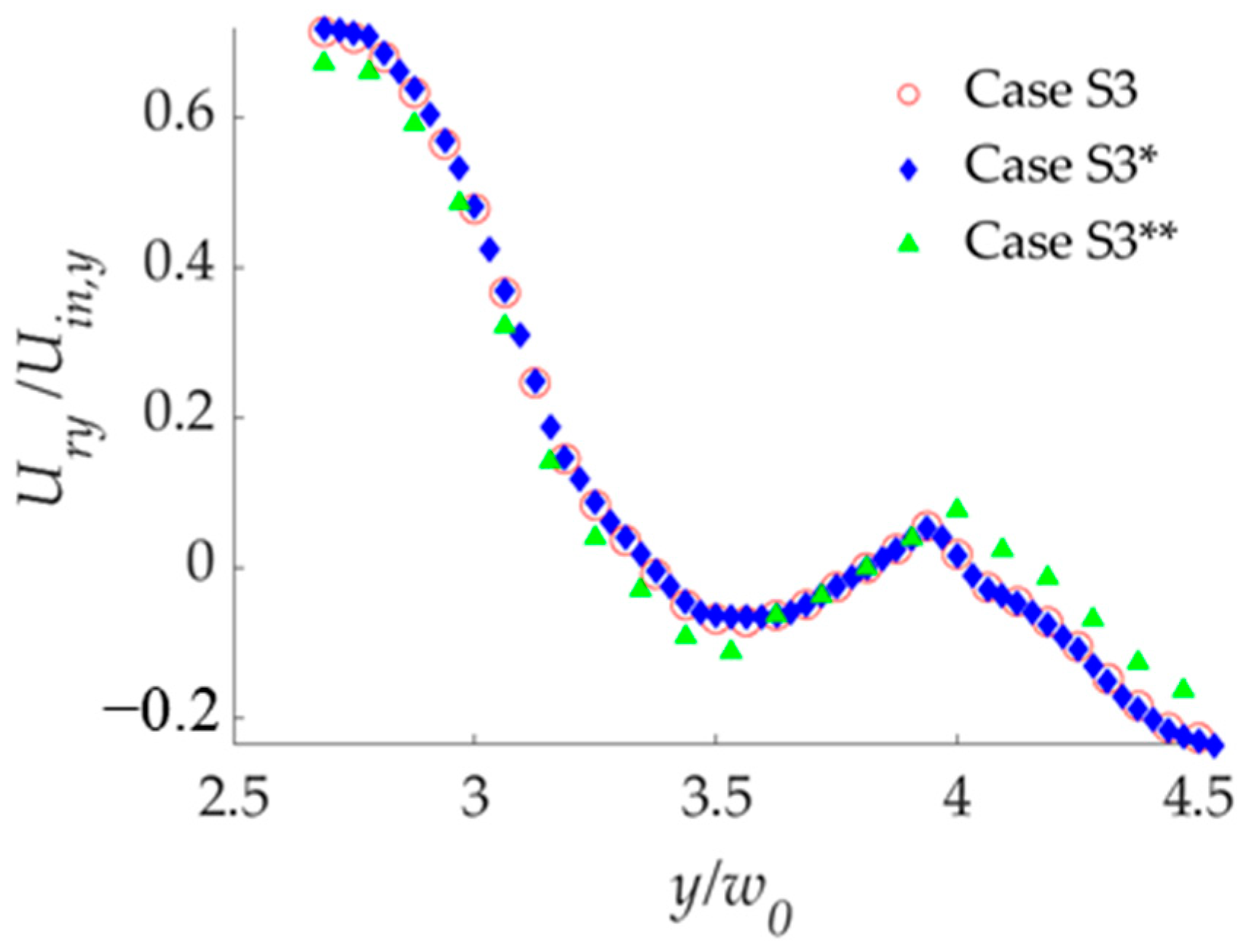
To verify the sensitivity of the grid size, Cases S3**, S3, and S3* were selected with the minimum grid size of 6 mm, 4 mm, and 2 mm, respectively, considering the source height h0 = 2 cm. The results of Case S3 are almost identical to Case S3* and Case S3**, as shown in Figure 2. Therefore, given the constraints imposed by computational resources, the model with the minimum grid size of 4 mm was selected. The G series cases require approximately 7 million grids, while the S series cases need about 8 million grids.

2.5.2. Comparison between Present Simulation and Experimental Data

We compared the numerical simulation results with the experimental results in [26]. The accuracy was evaluated using the below skill score [28]:
S S = 1 i = 1 C o u n t v LES v PIV 2 i = 1 C o u n t v PIV v PIV ¯ 2
where v LES is the computation result, v PIV is the experimental data, and v PIV ¯ is the mean value of series v PIV . The feasibility of the model is extremely high when the skill score is greater than 0.65, and the credibility of the model is poor when it is less than 0.2.
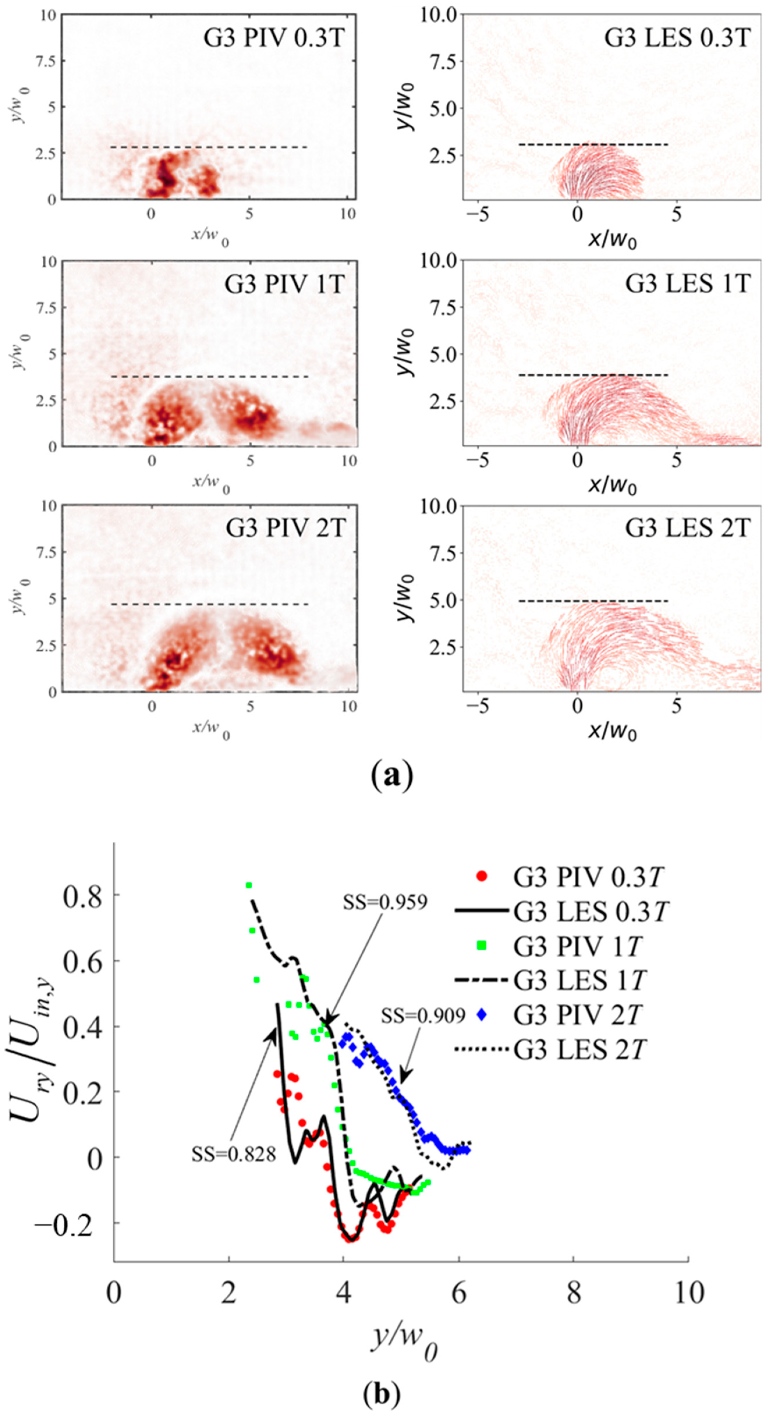
Figure 3a shows the horizontal velocity fields captured by particle image velocimetry (PIV) [26] for Case G3 at t = 0.3 T, 1 T, and 2 T, respectively, where T is the rotation period of the case. The right column presents the corresponding computed results obtained by the LES. The distances from the black dashed lines to the x-axis in the 6 panels are the maximum widths of the river plume at that moment.
Figure 3b shows the PIV experimental results v PIV and computed data v LES of the offshore velocity in the center of the inlet at t = 0.3 T, 1 T, and 2 T for Case G3. U i n , y is the source velocity and U r y is the offshore velocity of the grid cell, with the plus or minus indicating the directions. The computed results of the maximum width and offshore velocity of the river plume are in good agreement with the experimental results. Therefore, the three-dimensional LES model used in this paper can correctly simulate the development of the river plume.

3. Results and Discussion

3.1. Plume Classification

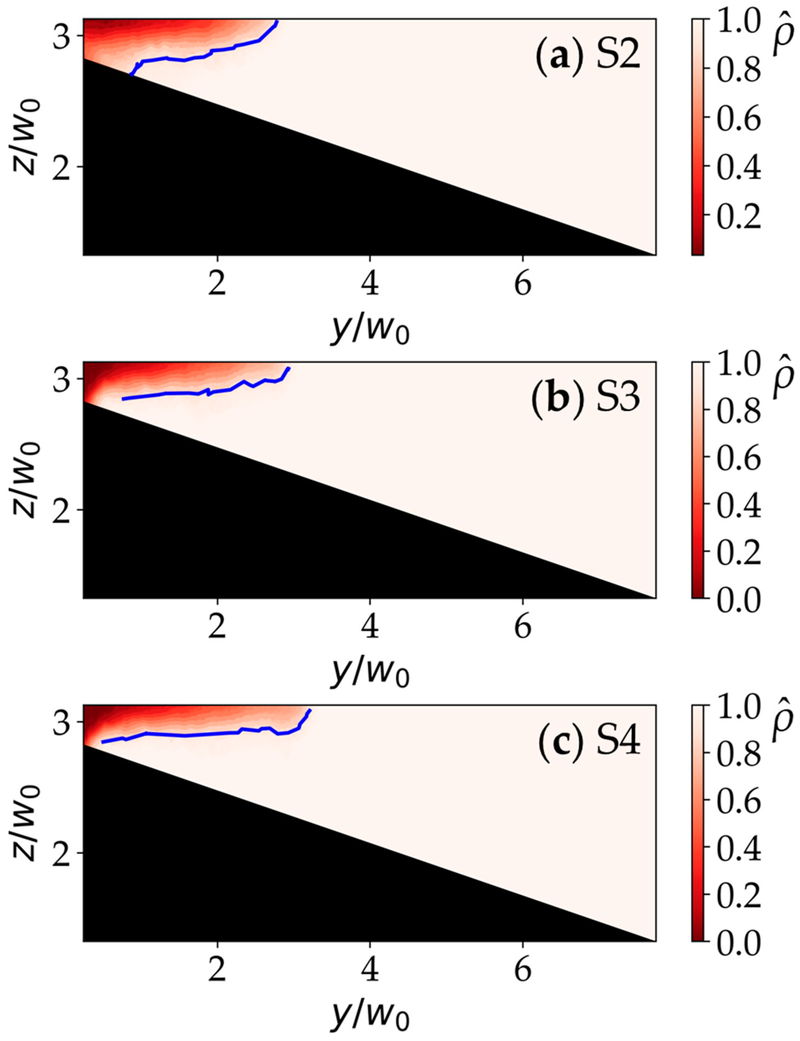
From a top view, the inflow of freshwater in the northern hemisphere moves radially after flowing out of the estuary and is deflected to the right by the Coriolis force. The plume bulge presents an anticyclonic vortex and a geostrophic jet structure surrounding the vortex, and the fresh water gradually forms two parts [4]: a circulation vortex area staying near the estuary and a coastal current flowing downstream. As T increases, so does the Rossby number, and the inertial force of fluid movement becomes dominant, causing river plume morphology to change from a surface-advected type to a bottom-attached type. The numerical model accurately reflects this morphological transition. The equilibrium depth [29] is defined here as:
h g = 2 Q f g
For Cases S2–S4, h g equals 2.446 cm, 2.118 cm, and 1.730 cm, respectively. Therefore, for Case S4, h g is less than buoyant inflow depth h 0 , and the river plume is surface-advected. Figure 4a shows the bottom-attached plume.

3.2. Gradient Richardson Number

Stratification and shear have a significant impact on the turbulence variation in estuaries and coasts. Stratification is defined using the square of the Brunt-Väisälä frequency:
N 2 = g ρ s ρ z
where ρ s is the initial density and ρ is the mixed fluid density. N represents the frequency at which the water parcel oscillates around the neutral density position in an area where density varies linearly [30]. Assuming that the vertical velocity gradient is much larger than the horizontal gradient, the mean shear S is defined as:
S 2 = u z 2 + v z 2
Shear generates turbulence, while stratification transforms kinetic energy into potential energy from turbulence in opposite ways. The Richardson number is often used for the comparison between shearing and stratification, and the gradient Richardson number is defined as [30]:
R i g = N 2 S 2
R i g = 0.25 is the critical value that distinguishes between subcritical and supercritical flows and indicates significant differences in instability morphology and mixing effectiveness at the interface. A larger R i g indicates that the adjacent layers are stable, while the opposite means that the velocity shear at the interface can overcome the limitations of stratification and produce shear instability.
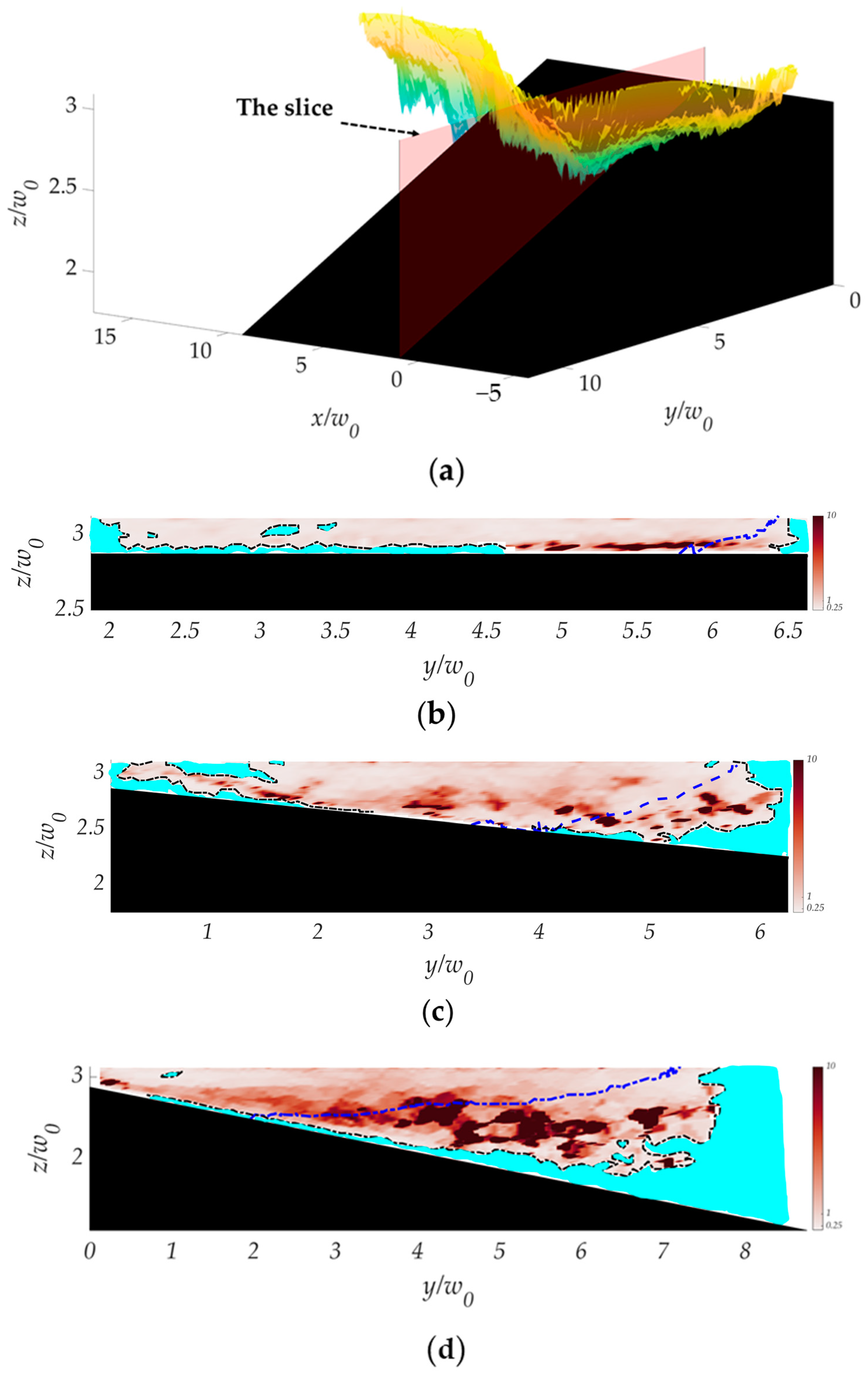
Taking the lateral profiles for Case A1, Case G2, and Case S4 as examples, Figure 5b–d show the lateral profiles of R i g . The black area corresponds to the bottom slope. The outer contour of the current plume bulge accurately delineates the external region where R i g < 0.25 , while in the majority of the internal region of the plume bulge, R i g 0.25 indicates strong stratification. The region near the wall exhibits higher rotational kinetic energy, resulting in stronger shear and hence a lower R i g . Inside the plume bulge, R i g near the bottom slope is more likely to be less than 0.25 compared to near the top. This is partly due to the inflow density ρ w being lower than that of the ambient fluid ρ s , causing upwelling of the inflowing fluid. For Case A1, based on the extremely small slope, the vertical convective space of the river plume is more constrained, with stronger offshore thrust near the wall. For Case G2, it is necessary to consider the acceleration effect of the bottom slope, which is discussed further in Section 3.5. Additionally, in Case A1, there are a few regions in the interior where R i g < 0.25 . Overlaying these adjacent cross-sections in the third dimension yields the corresponding three-dimensional structure with shear instability. A very small area of cyan parts inside the contour for Case S4 presents stronger stratification compared with the other two cases.
Taking R i g as an example, the current numerical simulation complements the previous experimental study by addressing the lack of vertical profile analysis. It provides a more intuitive understanding of the three-dimensional structure of a river plume. While PIV experiments can construct quasi-three-dimensional structures using field data obtained at each layer, the present numerical simulation directly provides three-dimensional structures, as seen in Figure 5a.

3.3. Effect of Reduced Gravity on River Plume Morphology

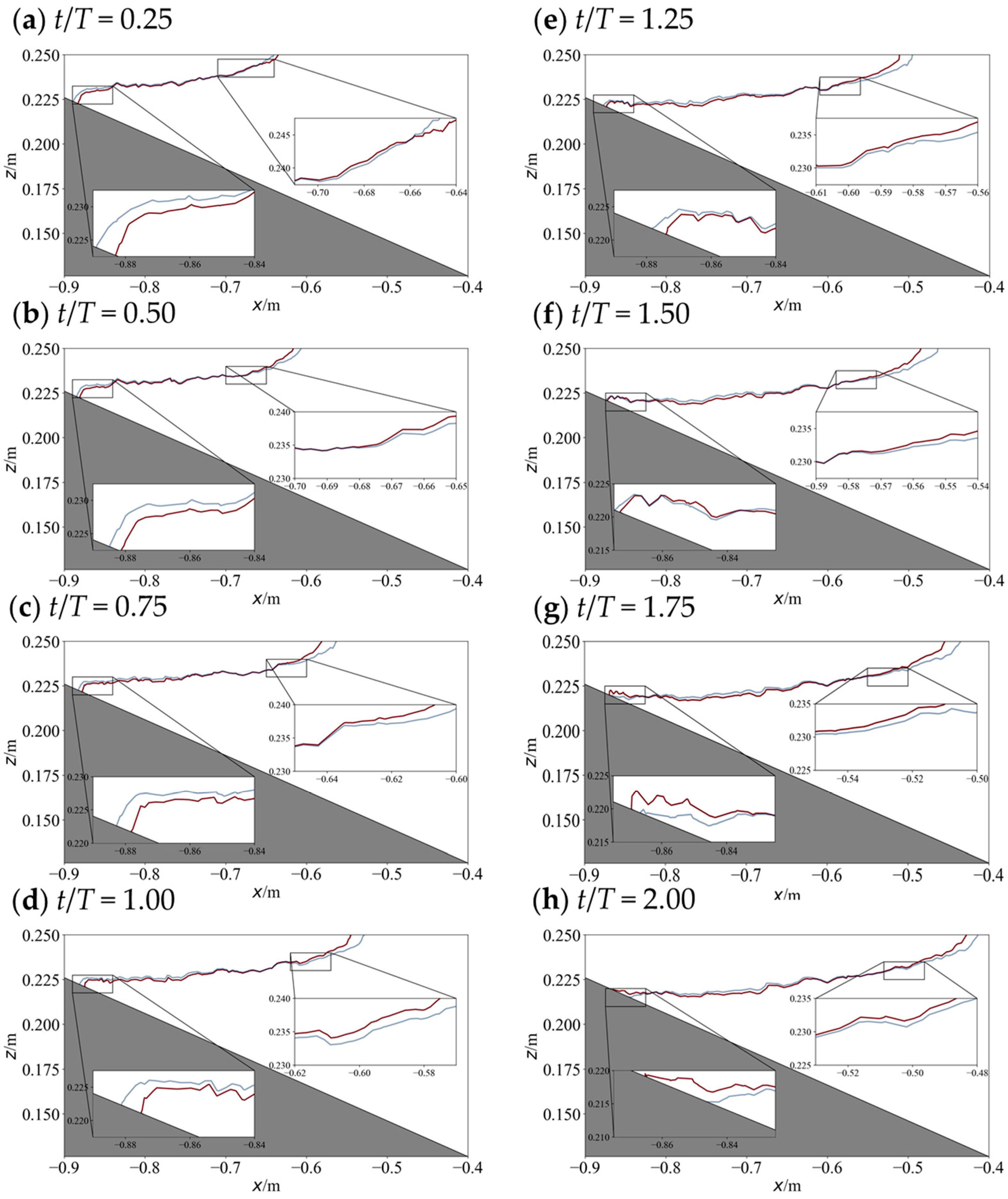
The salinity field of the lateral profile was converted into a density field, facilitated by the transformation relationship between the density of saline and temperature under a standard atmosphere proposed by Millero and Huang [31]. The normalized processing of the NaCl aqueous solution density was performed using the formula ρ ^ = ρ ρ w / ρ s ρ w . The red and blue lines in Figure 6 are the contour lines, with a value of 0.8. There is little difference between Case S1 and Case S4, as shown in Figure 6a−h. From Figure 6b−e, it can be found that at the same vertical height, in the horizontal direction, the river plume for Case S4, with a larger reduced gravity, spreads faster near the top than that for Case S1. However, near the bottom slope, the river plume for Case S4 gradually spreads faster than that for Case S1 starting in Figure 6f−h, which indicates that larger reduced gravity does promote the spread of river plumes, especially in the upper layer of ambient flow, but it is not as intuitive as the influence of the rotation period discussed in Section 3.1 on the structure of river plumes.

3.4. How the Salinity Field Varies with Time under Different Shelf Slopes

A right trapezium with a height of 90 cm is used to simulate the real continental shelf. When the slope is 5 × 10⁻⁴, the difference between parallel sides of the trapezium is only 0.045 cm, which cannot be achieved in laboratory experiments. This demonstrates the necessity of performing numerical simulations.
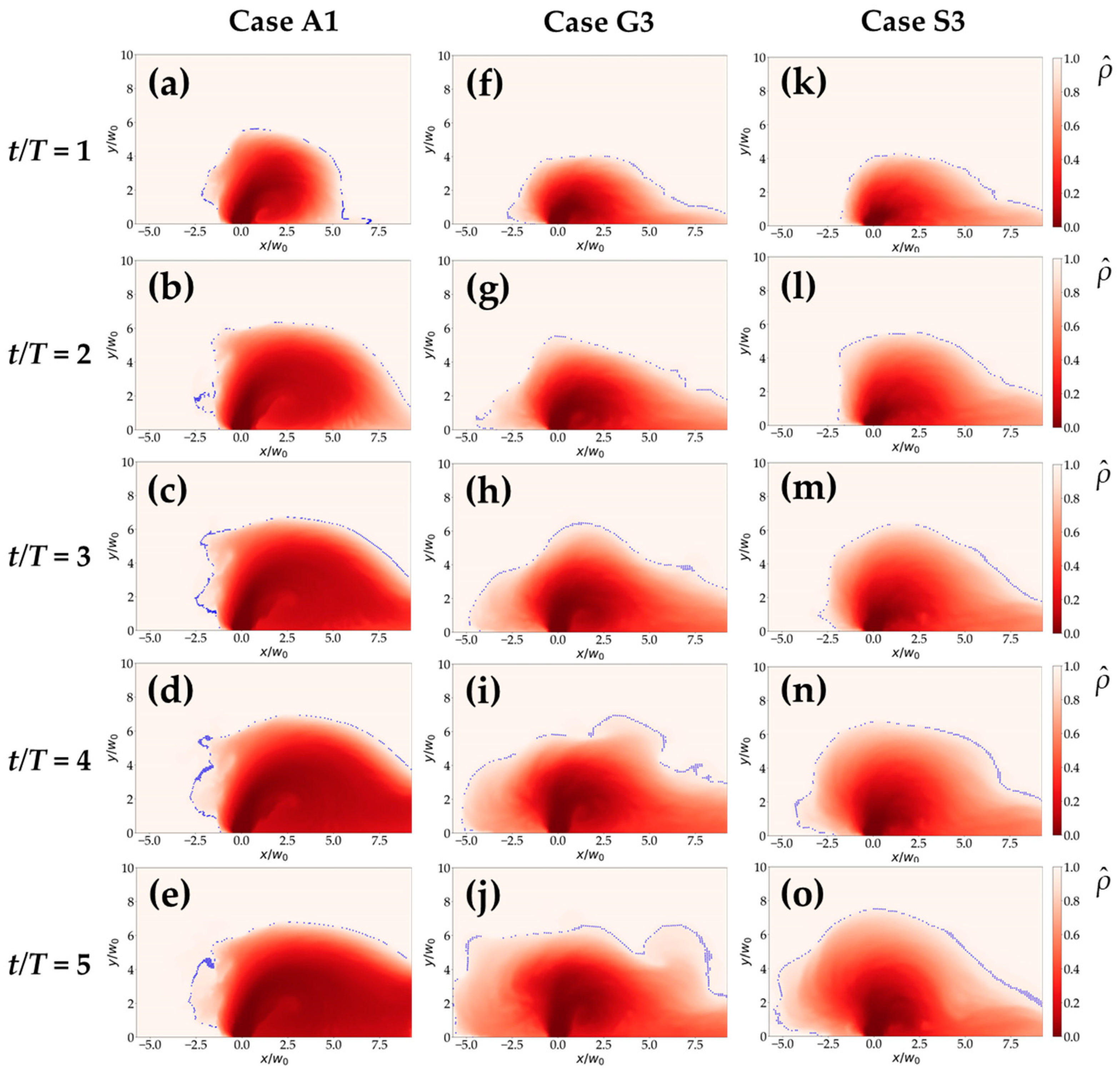
Figure 7 shows the schematic diagram of the dimensionless density field on the top of the three slopes at T = 40 s and g’ = 7 cm2/s. The definition of the dimensionless density field is given in Section 3.3. The blue scattered points correspond to dimensionless densities ρ ^ in the range (0.945, 0.955). In Figure 7i–j for Case G3, cyclone vortices can be seen clearly, and the river plume is highly unstable. However, in Figure 7n–o for Case S3, the structure of the geostrophic jet gradually develops on the left side of the inlet, and the overall stability is maintained well. Case A1, which cannot be obtained experimentally, shows the instability of the geostrophic jet structure to a certain extent, in which some fresh water is thrown out to the left during the process.
BIN = θ R o i n
θ = g α L b f 2
L b = 2 Q g f 3 0.25
In the above formula, θ represents the instability parameter, while L b denotes the Rossby radius. When the bulk Richardson number (BIN) [18] is less than 0.8, the development of river plumes is predominantly influenced by rotational kinetic energy. Consequently, it produces extra cyclonic vortices, aligning well with the characteristics of the bottom-attached plume, as seen in Figure 7i. From a parameter-calculation perspective, it is observed that the BIN values for Case G3 and Case S3 are situated on either side of the 0.8 threshold. Meanwhile, due to its gentle slope, Case A1 necessitates a BIN value below 0.8, thus maintaining characteristics consistent with a bottom-attached plume. Nevertheless, it is noteworthy that no distinct cyclonic structure is discernible outside the bulge. We posit that as the bottom slope approaches 0, the vertical movement of fresh water becomes spatially constrained. This results in heightened offshore movement, corresponding to a plume maximum width greater than that observed in the other two cases at the same time period, as seen in Figure 7a,f,k. Subsequently, a coastal current emerges, albeit with a noticeable delay associated with the slope and the rotation period, and the horizontal terrain adjustments necessitate an extended development period. However, when compared to the red depth of the other two cases at the same time, Case A1 exhibits pronounced kinetic energy within the plume bulge.
In terms of the significance of conducting numerical simulations, the supplemented Case A1 expands the parameter space that cannot be reached in laboratory experiments. The BIN parameter is still insufficient in terms of measuring the stability of the plume structure. The instability of Case A1 is not as obvious as that of Case G3.

3.5. Analysis of the Statistical Distribution of the Maximum Widths

The top salinity fields were normalized by dividing each grid cell’s salinity by the initial salinity value of the ambient fluid. After screening out the grid cells with dimensionless salinity in 0.885–0.915, the cell with the maximum offshore distance was taken as the point with the maximum width.
Figure 8a,b illustrates that only altering the reduced gravity does not induce substantial modifications in the overall distribution pattern of horizontal coordinates for a plume’s maximum width. At a specific adjacent moment, approximately 1.5 T, the x-coordinate value changes sharply, as seen in Figure 8a. It shows that the cyclonic vortex begins to separate from the bulge, as seen in Figure 7f–h. The distribution pattern for Case S3 develops an “M” shape, while Case A1 shows a continuous trend of movement along the same direction as the coastal current’s. Cases A1, G3, and S3 have the same T and g’, but the slope value of 0.1 in Case S3 is located between 5 × 10⁻⁴ and 0.2. The obviously different distributions of maximum widths in the above three cases demonstrate the non-negligible influence of the shelf slope on the development of plume structure. On the other hand, similar sections also exist in these three cases, while two analogous parts were outlined with dashed boxes of the same color, corresponding to black dotted lines and red dashed lines in Figure 8. Based on the proportion of similar parts in the overall distribution pattern, we can determine a fundamental recognition of the temporal sequence of plume development in the above cases solely with different slope values. Larger shelf slopes accelerate the development of river plumes in a more evident way, as greater slope values correspond to larger accelerations, which is quite intuitive. In addition, an increase in bed slope also highlights other hydrodynamic phenomena, like vortices and ski jumps [32,33].
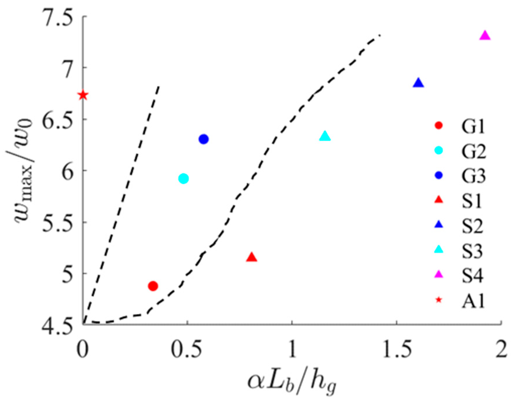
Regarding the bottom slope parameter α L b / h g [18,34] as the x axis and the dimensionless plume maximum width during the stationary phase as the y axis, the scattered distribution of the above eight typical cases is plotted, as shown in Figure 9. It can be seen that the bottom slope parameter distinguishes three kinds of shelf slopes. Here, the stationary phase corresponds to 3–10 rotation periods. The recirculating bulge grows unstable after 10 T in most cases without a slope, while the plume maximum width increases dramatically in the exponential phase (0–3 T) [5].

4. Conclusions

  • The numerical model effectively replicates the evolution process of river plumes and the inherently unstable vortex structure observed in laboratory experiments conducted under windless and rainless conditions. It extends the parameter spaces that are inaccessible through conventional laboratory experiments, as demonstrated by employing an exceedingly gentle slope. Meanwhile, current numerical simulations complement the previous experimental study by addressing the lack of vertical profile analysis.
  • The outline of the plume bulge quite accurately delineates the external region where the gradient Richardson number is less than 0.25, indicating strong shear, while in the majority of the internal region of the plume bulge, it is larger than 0.25. The region near the wall exhibits a lower gradient Richardson number, considering higher rotational kinetic energy. Inside the plume bulge, the gradient Richardson number near the bottom slope is more likely to be less than 0.25 compared to near the top.
  • The bulge instability number evaluates the stability of a river plume from a holistic perspective. For gentle slope cases, designating certain river plumes as unstable does not necessarily imply that extensive regions within the bulge exhibit weak stratification. On the other hand, the area of the region with weak stratification is quite small for steep slope cases, which further substantiates its characterization as a stable river plume. Steep slopes correspond to a larger distribution area and color depth in strong stratification regions.
  • A larger reduced gravity does promote the propagation of river plumes, especially in the upper layer of water, but it is not as intuitive as the influence of rotation period and slope on plume structure. When the shelf slope approaches 0, the offshore movement becomes stronger while the alongshore coastal current comes into being with a delay related to the slope and the rotation period.
  • Compared with the steep slope case and the extremely gentle slope case, with the same rotation period and reduced gravity, the horizontal coordinate of the point corresponding to the maximum width in the gentle slope case at about t = 1.5 T changed significantly. However, similar sections also exist in these three cases. A larger shelf slope accelerates the development of river plumes, evidently.
In summary, this paper introduces a numerical model for investigating plume characteristics based on a modified solver for solving governing equations with the Boussinesq approximation in a single rotating frame, which enriches the existing numerical models of river plumes. The lateral profiles of the gradient Richardson number obtained from the research provide a basis for further exploration of stratification and shear. Meanwhile, this model holds potential for application in the exploration of river plumes in other regions.

Author Contributions

Conceptualization, J.Z. and Y.Y.; methodology, J.Z., K.H. and Y.-T.L.; modeling, J.Z.; investigation, J.Z. and K.H.; writing—original draft preparation, J.Z. and K.H.; writing—review and editing, Y.Y., Y.-T.L. and D.H.; visualization, J.Z. and D.H.; supervision, Y.-T.L.; funding acquisition, Y.Y. All authors have read and agreed to the published version of the manuscript.

Funding

This research was funded by the Zhejiang Provincial Natural Science Foundation of China under Grant No. LZ24D060002, Key Laboratory of Estuary and Coast of Zhejiang Province (No. ZIHE21002), the Science Foundation of Donghai Laboratory (Grant No. DH-2022KF01016), the National Natural Science Foundation of China (No. 61041876089), and the Science Foundation of Hainan Observation and Research Station of Ecological Environment and Fishery Resource in Yazhou Bay (No. HNOBYZ2201).

Institutional Review Board Statement

Not applicable.

Informed Consent Statement

Not applicable.

Data Availability Statement

Data are contained within this article.

Acknowledgments

The authors thank Xu Chen, Yujun Yu, and Guofeng Fu from Ocean University of China for their help building the rotating tank, and thank Haochen Song, who assisted with the data collection.

Conflicts of Interest

The authors declare no conflicts of interest.

References

  1. Griffiths, R.W. Gravity Currents in Rotating Systems. Annu. Rev. Fluid Mech. 1986, 18, 59–89. [Google Scholar] [CrossRef]
  2. Saunders, P.M. The Instability of a Baroclinic Vortex. J. Phys. Oceanogr. 1973, 3, 61–65. [Google Scholar] [CrossRef]
  3. Horner-Devine, A.R.; Fong, D.A.; Monismith, S.G.; Maxworthy, T. Laboratory experiments simulating a coastal river inflow. J. Fluid Mech. 2006, 555, 203–232. [Google Scholar] [CrossRef]
  4. Nof, D.; Pichevin, T. The Ballooning of Outflows. J. Phys. Oceanogr. 2001, 31, 3045–3058. [Google Scholar] [CrossRef]
  5. Chapman, D.C.; Lentz, S.J. Trapping of a Coastal Density Front by the Bottom Boundary Layer. J. Phys. Oceanogr. 1994, 24, 1464–1479. [Google Scholar] [CrossRef]
  6. Garvine, R.W. Physical features of the Connecticut River outflow during high discharge. J. Geophys. Res. (1896–1977) 1974, 79, 831–846. [Google Scholar]
  7. Rabalais, N.N.; Turner, R.E.; Wiseman, W.J. Gulf of Mexico Hypoxia, A.K.A. “The Dead Zone”. Annu. Rev. Ecol. Syst. 2002, 33, 235–263. [Google Scholar] [CrossRef]
  8. Münchow, A.; Garvine, R.W. Dynamical properties of a buoyancy-driven coastal current. J. Geophys. Res. Ocean. 1993, 98, 20063–20077. [Google Scholar] [CrossRef]
  9. Mudroch, A. Distribution of Major Elements and Metals in Sediment Cores from the Western Basin of Lake Ontario. J. Great Lakes Res. 1983, 9, 125–133. [Google Scholar] [CrossRef]
  10. Yankovsky, A.E.; Hickey, B.M.; Münchow, A.K. Impact of variable inflow on the dynamics of a coastal buoyant plume. J. Geophys. Res. Ocean. 2001, 106, 19809–19824. [Google Scholar] [CrossRef]
  11. Fong, D.A.; Geyer, W.R. The Alongshore Transport of Freshwater in a Surface-Trapped River Plume. J. Phys. Oceanogr. 2002, 32, 957–972. [Google Scholar] [CrossRef]
  12. Chen, S.-N.; Geyer, W.R.; Hsu, T.-J. A Numerical Investigation of the Dynamics and Structure of Hyperpycnal River Plumes on Sloping Continental Shelves. J. Geophys. Res. Ocean. 2013, 118, 2702–2718. [Google Scholar] [CrossRef]
  13. Fofonova, V.; Kärnä, T.; Klingbeil, K.; Androsov, A.; Kuznetsov, I.; Sidorenko, D.; Danilov, S.; Burchard, H.; Wiltshire, K.H. Plume spreading test case for coastal ocean models. Geosci. Model Dev. 2021, 14, 6945–6975. [Google Scholar] [CrossRef]
  14. Brasseale, E.; MacCready, P. The Shelf Sources of Estuarine Inflow. J. Phys. Oceanogr. 2021, 51, 2407–2421. [Google Scholar] [CrossRef]
  15. Xiao, Y.; Yang, Z.; Wang, F.; Liu, M. Large eddy simulation of the hydrodynamic behavior of horizontal side jets in compound open channels with vegetated floodplain. Environ. Sci. Pollut. Res. 2020, 27, 7967–7983. [Google Scholar] [CrossRef] [PubMed]
  16. Hamlington, P.E.; Meehan, M.A.; Wimer, N.T. Richardson and Reynolds Number Effects on the near Field of Buoyant Plumes: Temporal Variability and Puffing. J. Fluid Mech. 2022, 950, A24. [Google Scholar]
  17. Shi, H.; Negretti, M.E.; Chauchat, J.; Blanckaert, K.; Lemmin, U.; Barry, D.A. Unconfined Plunging of a Hyperpycnal River Plume Over a Sloping Bed and Its Lateral Spreading: Laboratory Experiments and Numerical Modeling. Water Resour. Res. 2022, 58, e2022WR032633. [Google Scholar] [CrossRef]
  18. Yuan, Y.; Tan, X.; Lin, Y.-T. Effect of sloping bottom on river plume dynamics on a laboratory-scale rotating table. Front. Mar. Sci. 2023, 10, 1126088. [Google Scholar] [CrossRef]
  19. Mayeli, P.; Sheard, G.J. Buoyancy-driven flows beyond the Boussinesq approximation: A brief review. Int. Commun. Heat Mass Transfer 2021, 125, 105316. [Google Scholar] [CrossRef]
  20. Balachandar, S.; Cantero, M.I.; Garcia, M.H. High-resolution simulations of cylindrical density currents. J. Fluid Mech. 2007, 590, 437–469. [Google Scholar]
  21. Rouhnia, M.; Strom, K.; Liu, X. Experiments and modeling of density instabilities driven by interface shear and their influence on removal of sediment from buoyant plumes. In Proceedings of the International Conference on Fluvial Hydraulics, St. Louis, MO, USA, 10–14 July 2016. [Google Scholar]
  22. Lorenzis, L.D.; Düster, A.; Guazzelli, É.; Rammerstorfer, F.G.; Wall, W.A.; Schrefler, B.; Serafini, P. Modeling in Engineering Using Innovative Numerical Methods for Solids and Fluids; Springer: Cham, Switzerland, 2020. [Google Scholar]
  23. Launder, B.E.; Reece, G.J.; Rodi, W. Progress in the development of a Reynolds-stress turbulence closure. J. Fluid Mech. 1975, 68, 537–566. [Google Scholar] [CrossRef]
  24. Von Kármán, T. Mechanical Similitude and Turbulence; National Advisory Committee for Aeronautics: Washington, WA, USA, 1931. [Google Scholar]
  25. Popovac, M.; Hanjalic, K. Compound Wall Treatment for RANS Computation of Complex Turbulent Flows and Heat Transfer. Flow Turbul. Combust. 2007, 78, 177–202. [Google Scholar] [CrossRef]
  26. Song, H.; Yuan, Y.; Lin, Y.-T.; Wang, Y.; Song, J. Laboratory investigation of the plume-to-plume interaction in a rotating tank. Phys. Fluids 2023, 35, 126608. [Google Scholar] [CrossRef]
  27. Montagna, P.A.; Palmer, T.A.; Pollack, J.B. Hydrological Changes and Estuarine Dynamics, 1st ed.; SpringerBriefs in Environmental Science; Springer: New York, NY, USA, 2012; Volume 8, p. 94. [Google Scholar]
  28. Zhu, L.; He, Q.; Shen, J.; Wang, Y. The influence of human activities on morphodynamics and alteration of sediment source and sink in the Changjiang Estuary. Geomorphology 2016, 273, 52–62. [Google Scholar] [CrossRef]
  29. Yankovsky, A.E.; Chapman, D.C. A Simple Theory for the Fate of Buoyant Coastal Discharges. J. Phys. Oceanogr. 1997, 27, 1386–1401. [Google Scholar] [CrossRef]
  30. Turner, J.S. Buoyancy Effects in Fluids, 1st ed.; Cambridge University Press: Cambridge, UK, 1973; p. 382. [Google Scholar]
  31. Millero, F.J.; Huang, F. The density of seawater as a function of salinity (5 to 70 g kg−1) and temperature (273.15 to 363.15 K). Ocean. Sci. 2009, 5, 91–100. [Google Scholar] [CrossRef]
  32. Tafarojnoruz, A.; Lauria, A. Large Eddy Simulation of the Turbulent Flow Field around a Submerged Pile within a Scour Hole under Current Condition. Coast. Eng. J. 2020, 62, 489–503. [Google Scholar] [CrossRef]
  33. Lauria, A.; Alfonsi, G.; Tafarojnoruz, A. Flow Pressure Behavior Downstream of Ski Jumps. Fluids 2020, 5, 168. [Google Scholar] [CrossRef]
  34. Avicola, G.; Huq, P. Scaling Analysis for the Interaction between a Buoyant Coastal Current and the Continental Shelf: Experiments and Observations. J. Phys. Oceanogr. 2002, 32, 3233–3248. [Google Scholar] [CrossRef]
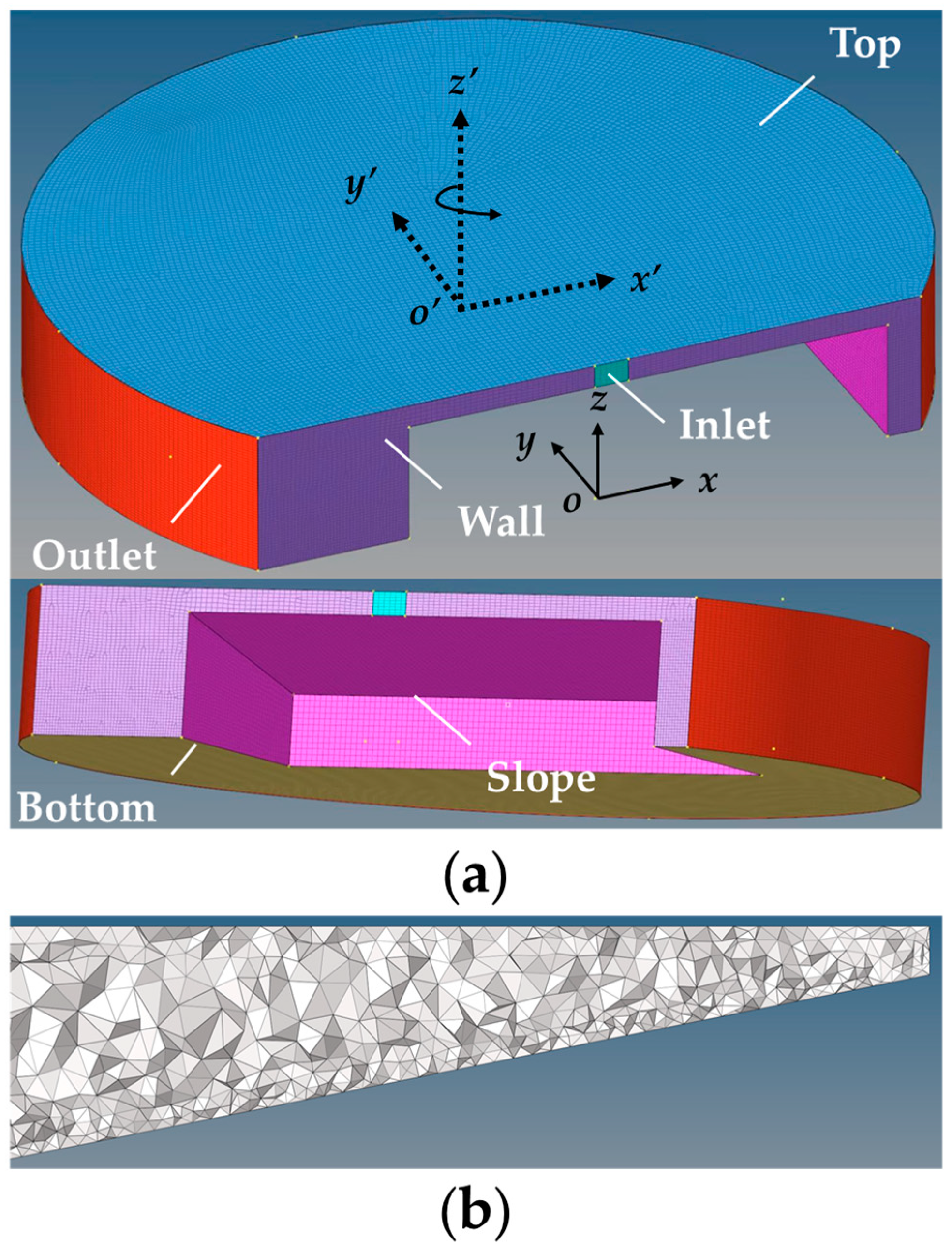
Figure 1. Schematic diagram of the model: (a) numerical model; (b) meshing. Coordinate values are determined using a plane rectangular coordinate system (oxyz). The rotation axis oz′ traverses the central point of the circle, exhibiting a counterclockwise orientation.
Jmse 12 00321 g001
Figure 2. Comparative schematic of the offshore velocity for Case S3 on 3 types of grid sizes. The minimum grid size is set to 2 mm in S3*, 6 mm in S3**, and 4 mm in S3.
Jmse 12 00321 g002
Figure 3. Comparison between the numerical results and the experimental results in [26] for Case G3: (a) maximum width; (b) offshore velocity. The distance between the dashed line and the x-axis in the 6 panels of Figure 3a denotes corresponding maximum plume width.
Jmse 12 00321 g003
Figure 4. Density profiles of the river plumes with 3 types of rotation periods at t = 10 s. The black area corresponds to the bottom slope. The saline density is normalized by ρ ^ = ρ ρ w / ρ s ρ w .
Jmse 12 00321 g004
Figure 5. Typical lateral profiles of the gradient Richardson number: (a) the location of the slice; (b) Case A1 at t = 5 T; (c) Case G2 at t = 3 T; (d) Case S4 at t = 2 T. In Figure 5b–d, the cyan parts are the regions where Rig < 0.25, while the blue dashed lines are the contours of the plume bulge, whose dimensionless salinity is located at (0.885, 0.915).
Jmse 12 00321 g005
Figure 6. Schematic diagram of lateral profiles. Case S1 corresponds to the red solid line, while Case S4 corresponds to the blue solid line.
Jmse 12 00321 g006
Figure 7. Schematic diagram of the top dimensionless density field: α = 5 × 10⁻⁴ (ae); α = 0.1 (fj); α = 0.2 (ko). The blue dots outline the contour of the bulge.
Jmse 12 00321 g007
Figure 8. Schematic diagram of the distribution of plume maximum width. Two analogous parts were outlined with dashed boxes of the same color, corresponding to the black dotted lines and red dashed lines.
Jmse 12 00321 g008
Figure 9. The relationship between the plume maximum width and the bottom slope parameter during the stationary phase.
Jmse 12 00321 g009
Table 1. Parameters of numerical simulations.
Case No.αT (s)ρsal (g/cm3)ρw (g/cm3)g′ (cm/s2)RoinFrin
G10.1301.0036430.9980105.50.930.94
G20.1401.0036430.9980105.51.240.94
G30.1401.0046600.9974947.01.240.84
A15 × 10−4401.0046600.9974947.01.240.84
S10.2601.0041450.9985095.51.870.94
S20.2301.0046600.9974947.00.930.84
S30.2401.0046600.9974947.01.240.84
S3*0.2401.0046600.9974947.01.240.84
S3**0.2401.0046600.9974947.01.240.84
S40.2601.0046600.9974947.01.870.84
The numbers following G, A, and S in the “Case No.” column are used for numbering only and have no physical significance, while A, G, and S represent extremely gentle slope, gentle slope, and steep slope, respectively. The minimum grid size is set to 2 mm in S3*, 6 mm in S3**, and 4 mm in the other cases.
Disclaimer/Publisher’s Note: The statements, opinions and data contained in all publications are solely those of the individual author(s) and contributor(s) and not of MDPI and/or the editor(s). MDPI and/or the editor(s) disclaim responsibility for any injury to people or property resulting from any ideas, methods, instructions or products referred to in the content.