Abstract
Annually, hundreds of individuals tragically lose their lives at sea due to shipwrecks or aircraft accidents. For search and rescue personnel, the task of locating the debris of a downed aircraft in the vastness of the ocean presents a formidable challenge. A primary task these teams face is determining the search area, which is a critical step in the rescue operation. The movement of aircraft wreckage on the ocean surface is extremely complex, influenced by the combined effects of surface winds, waves, and currents. Establishing an appropriate drift motion prediction model is instrumental in accurately determining the search area for the wreckage. This article initially conducts maritime drift observation experiments on wreckage, and based on the results of these experiments, analyzes the drift characteristics and patterns of the debris. Subsequently, employing a wealth of observational experimental data, three types of drift prediction models for the wreckage are established using the least squares method. These models include the AP98 model, the dynamics model, and an improved model. In conclusion, the effectiveness and accuracy of the three models is evaluated and analyzed using Monte Carlo techniques. The results indicate that the probability of positive crosswind leeway (CWL) is 47.4%, while the probability of negative crosswind leeway (CWL) is 52.6%. The jibing frequency is 7.7% per hour, and the maximum leeway divergence angle observed is 40.4 degrees. Among the three drift prediction models, the refined AP98 drift model demonstrates the highest forecasting precision. The findings of this study offer a more accurate drift prediction model for the search of an aircraft lost at sea. These results hold significant guiding importance for maritime search and rescue operations in the South China Sea.
1. Introduction
On 1 June 2009, Air France Flight 447 from Rio de Janeiro to Paris met with an accident over the Atlantic Ocean. The first debris was discovered on June 8 at sea, but it was not until 2 May 2011 that the flight’s black boxes were located in the relevant maritime area. On 8 March 2014, Malaysia Airlines Flight MH370 from Kuala Lumpur to Beijing disappeared over the southern Indian Ocean. The first piece of wreckage was not found until 29 July 2015, on the shores of Réunion Island, located in the western Indian Ocean. In marine aviation disasters, the aircraft fuselage breaks into fragments, some of which sink to the ocean floor, while others, being less dense than seawater, remain afloat. Locating these floating fragments is crucial for determining the crash area and facilitating the search for the flight recorders [1,2,3].
Floating debris at sea undergoes a drift motion under the combined influence of wind, waves, and ocean currents [4,5,6,7,8]. Establishing appropriate drift motion models is crucial for accurately forecasting the drift trajectories of floating debris. In response to this need, scholars have undertaken a series of research initiatives aimed at predicting the drift paths of maritime floating debris. Kubota studied the accumulation mechanism of floating Marine debris in the North Pacific Ocean, especially north of the Hawaiian Islands, and simulated the sea surface currents composed of the Stokes drift, Ekman drift, and geostrophic current, and the results showed that Marine debris gathered north of the Hawaiian Islands [9]. Martinez identified that debris in the South Pacific ultimately converges in the eastern–central region of the South Pacific Subtropical Gyre [10]. Conversely, Dobler posited that considering the influence of the Stokes drift on floating objects, the accumulation area of debris in the southern Indian Ocean would shift towards the South Atlantic [11]. Maximenko utilized five different ocean models to simulate the movement of debris from the 2011 Japanese tsunami, finding that the trajectories of the floating debris varied under different wind speed conditions [12]. Following the Malaysia Airlines Flight MH370 disaster, scholars from various countries extensively engaged in simulating the drift trajectory of the aircraft’s wreckage in the search for the missing plane. Gao and colleagues developed a prediction model for the drift trajectory of objects in the southern Indian Ocean based on the leeway drift theory and the Monte Carlo method. They used three sets of wind drift coefficients to predict the drift trajectory over 500 days. The predicted results were largely consistent with the analysis of the surface drifting buoy trajectories, demonstrating the reliability of the drift trajectory prediction model [13]. Jansen and colleagues proposed the use of numerical simulations with high-resolution oceanic and meteorological data to predict the movement of floating debris in accidents. They created different models by choosing various starting positions and wind resistance parameters, combining these models into a superensemble to predict the debris distribution at different times [3]. Durgadoo and colleagues utilized a state-of-the-art ocean circulation model to simulate currents, combined with a surface Stokes drift, to determine the potential paths of the debris. Their results highlighted the significance of the Stokes drift and the buoyancy characteristics of objects in simulating drift trajectories [14].
The aforementioned studies on the drift movements of floating marine debris have predominantly been conducted under large-scale spatiotemporal conditions, with minimal research focusing on the micro-level drift characteristics of the debris itself. The drift characteristics of different maritime floating objects at sea are different, the most obvious being that the coefficients in their drift models are quite different. These characteristics can be ascertained through maritime experimental methods. In 1999, Allen and Plourde pioneered the quantitative AP98 model, which is based on extensive maritime experimental results. This model, parameterized by the wind speed and wind-induced drift angle, established wind-induced drift equations for 63 types of search and rescue targets, including marine and aviation debris, thereby creating a comprehensive database of wind-induced drift characteristics for common search and rescue targets [15,16,17]. Based on a leeway model, Breivik summarized experimental schemes for the direct and indirect observation of drifting objects of different volumes, conducted field experiments on various types of targets such as oil drums, mines, and falling containers, and studied the wind drift coefficients of falling containers under different load ratios [18,19,20,21]. Brushett calibrated the wind drift coefficients for three common types of small boats in the Pacific Islands under downwind and crosswind conditions. They also conducted multiple experiments on kayaks (5.8 m) under different load conditions, revealing that the wind drift coefficients of kayaks varied between 7.71% and 4.40% for loads ranging from 1 to 13 persons [22]. Zhu carried out drift experiments on typical nearshore fishing vessels using direct observation methods, analyzing the drift characteristics and patterns of these vessels when unpowered at sea [23]. It is evident that scholars have been conducting maritime drift experiments to study the drift characteristics and patterns of common sea-borne targets [24,25]. However, there is still a relative scarcity of drift experiments for specific oceanic areas, especially regarding floating debris, which necessitates further research in this area.
The South China Sea, a region of frequent human activity and high risk of maritime accidents, necessitates conducting maritime drift experiments on floating debris. This research will contribute to the development of more accurate drift prediction models, thereby guiding maritime search and rescue efforts. This paper employs maritime experimental methods to study the drift characteristics of floating debris in the South China Sea. Initially, a series of maritime drift experiments with two different sizes of floating debris were conducted in the South China Sea to gather data on the drift characteristics of the debris and marine environmental conditions. Subsequently, based on the comprehensive maritime experimental data, three drift prediction models were established, including the AP98 leeway model, a dynamic drift model, and an improved drift model. Finally, the Monte Carlo technique was used to compare and evaluate the three drift prediction models, identifying the optimal model for predicting the drift of floating debris at sea. The results of this study provide technical support for predicting the drift of maritime floating debris and hold significant importance for maritime search and rescue operations in the South China Sea.
2. Theoretical Models and Methods
2.1. AP98 Leeway Model
In 1999, Allen and Plourde established the quantified AP98 model according to a multitude of maritime experimental results [15]. This model indicates that different types of floating objects at sea have distinct leeway characteristics. For most search and rescue targets (with lengths smaller than the wavelengths of ocean waves), the force exerted by the waves can be disregarded. The model rigorously defines ‘leeway’ as the drift movement of an object caused by surface winds (at a height of 10 m) and surface currents (0.3 to 1.0 m deep). The speed of the floating object can be represented as follows:
where is composed of the drift speed caused by surface currents, which is generally equivalent to the speed of the surface currents, and represents the drift velocity of the object induced by surface winds.
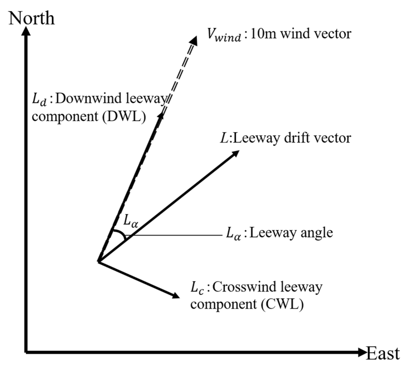
The early AP98 model struggled to accurately account for the variability in wind-induced drift angles, especially at low wind speeds. In 2005, Allen refined the model by decomposing the wind-induced drift velocity into two more robust components: the downwind velocity (DWL) and the crosswind velocity (CWL), as illustrated in Figure 1. He re-established the wind-induced drift equation accordingly. In this revised model, the probability of the crosswind velocity CWL veering left (−CWL) or right (+CWL) is the same [16].
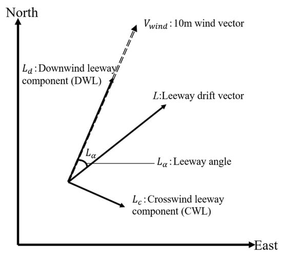
Figure 1.
The leeway L consists of a downwind component Ld and a crosswind component Lc.
In the AP98 model, the downwind velocity and the two perpendicular wind velocities in relation to wind speed can be expressed using three linear functions. The model contains nine parameters, representing the slope, intercept, and standard deviation for each of the three regression equations. The expressions are as follows:
where represents the component of the wind-induced drift velocity in the downwind direction, while and denote the components of the wind-induced drift velocity on the right and left side of the wind direction, respectively. These components are linearly related to the wind speed (referenced at a height of 10 m). The parameters , and represent the slope, intercept, and error term for the downwind direction component, respectively. Similarly, , ,, , and are the coefficients for the crosswind direction components.
2.2. Dynamics Drift Model
The model simplifies the forces of waves and neglects acceleration, positing that the motion of floating objects is influenced solely by ocean currents and wind. The part of the object below the waterline is affected by ocean currents, while the part above the waterline is influenced by wind forces. According to Newton’s third law of motion, when an object drifts at a steady speed, these two forces should be equal and opposite, summing to zero. The drift dynamics model can be represented by the following equation:
where , and respectively, represent the drift velocity, wind velocity, and current velocity. C is the drag coefficient, S denotes the cross-sectional area, and represents the density, with subscripts indicating air and water. From this, the following can be derived:
Here, . Let , and formula (4) can be expressed as follows:
where λ represents the current-induced drift motion coefficient, while (1 − λ) is the wind-induced drift coefficient. Given that , and in the above formula are vectors, for the ease of applying the least squares method for linear regression, the data for wind speed, current speed, and object speed are decomposed into components in the X (east) and Y (north) directions. Therefore, when modeling, it is necessary to perform linear regression separately for the coefficients in these two directions. The expression for the drift speed of the object in the dynamic drift model is as follows:
2.3. Improved Drift Model
The leeway model calculates the leeway speed by considering the current speed as the object’s current-induced drift velocity, neglecting the dissipation due to the drag force exerted by the water flow. In reality, the drift velocity caused by the current is not consistent with the current speed, leading to some error in the leeway drift model when calculating the leeway speed. The dynamics model treats the object’s drift velocity as the vector sum of the wind speed and current speed, deriving the coefficients affecting the current speed and wind speed through linear regression. However, it does not accurately account for the influence of wind speed on the drift direction, leading to imprecise predictions of the drift direction. Based on these considerations, this paper proposes an improved leeway drift model. The determination of the current-induced drift coefficient follows the approach of the dynamic drift model, while the leeway coefficient is determined using the method of the leeway drift model, resulting in more accurate calculations of the leeway velocity. The improved leeway drift model is expressed as follows:
Here, represents the object’s drift velocity, is the current velocity, is the leeway drift velocity, and k represents the drift coefficient derived from the dynamic drift mode. The leeway drift velocity is the same as expressed in Equation (2).
2.4. Monte Carlo Method
The Monte Carlo method, which employs random numbers to solve computational problems, is extensively used in computational physics, such as in particle transport calculations [26]. This paper utilizes the Monte Carlo method to simulate debris drift trajectories based on three models.
The drift motion equation of the AP98 leeway model is as follows:
The prediction equation for the drift trajectory in the dynamic model is as follows:
The prediction equation for the drift trajectory in the improved model is expressed as follows:
In the equation, represents the position of the maritime distress target, t is the drift time, is the initial moment of drift, and is the target’s drift velocity. When applying the Monte Carlo method, each sample sets up 1000 particles for the simulation. To account for the uncertainty caused by the errors present in leeway experiments, it is necessary to perturb the leeway coefficients. The perturbation formula for the leeway coefficient of the j th particle is as follows:
In the formula, and represent the model coefficients for the j th particle, and represents the coefficient perturbation for the j th particle, which is randomly selected from a normal distribution with a mean of 0 and a variance of 1 during calculation. Additionally, when using the Monte Carlo method to simulate the leeway drift model and the improved drift model, it is necessary to set the probability of positive crosswind (POPC) and the jibing frequency for the drifting target.
3. Maritime Drift Experiments
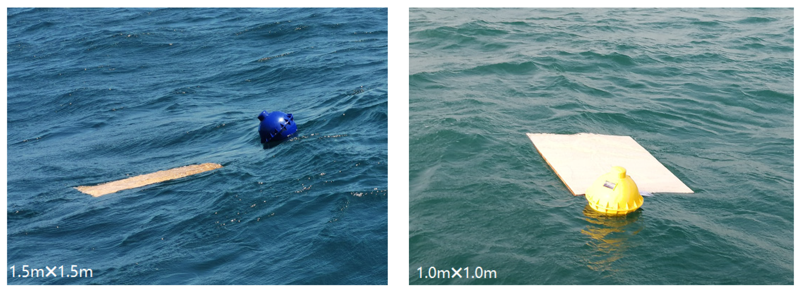
Drift experiments for debris were carried out in the waters of the Pearl River Estuary in the South China Sea (approximately between 113.0° E to 114.0° E longitude and 21.2° N to 22.0° N latitude). With the purpose of increasing the data amount and diversity of experiment samples, two different-sized wooden planks were used to simulate floating debris at sea. One piece of floating debris measured 1.5 m by 1.5 m, while the other measured 1.0 m by 1.0 m. Figure 2 illustrates these two pieces of floating debris used in the maritime drift experiment.

Figure 2.
The two pieces of debris used in the drift experiment.
During the debris drift experiment, the position of the experimental target and the corresponding sea currents, surface wind, and waves at that location were observed simultaneously. The real-time drift position of the debris was acquired using the LS-TB300MM (Shenzhen, China) tracking buoy. Sea currents were measured using a Nortek Signature ADCP acoustic Doppler current profiler operating at a frequency of 500 kHz. Surface wind data were observed using a 220WX weather station, and surrounding wave information was gathered using the LS-TB300MM wave observation buoy. The observation equipment is shown in Figure 3, and the relevant parameters of the observation equipment are listed in Table 1. The positioning tracking buoy, installed on the experimental target, drifted along with it, directly obtaining the target’s position information. The acoustic Doppler current profiler was fixed on a custom-made boat following the experimental target to collect surface current data from 0 m to 2 m. The multi-parameter weather station was mounted on the survey boat, approximately 10 m above the sea’s surface, which followed the experimental target to gather surface wind data. The wave observation buoy was connected to the custom-made boat with a rope to observe wave information around the experimental target. During the navigational observations, the relative distance between each measuring device and the experimental target did not exceed 50 m.

Figure 3.
Observation equipment for the drift experiment. (A) Tracking buoy, (B) acoustic Doppler current profiler, (C) multi-parameter weather station, and (D) small wave observation buoy.

Table 1.
Parameter table for observation equipment in the drift experiment.
The specific steps of the debris drift experiment are as follows:
- (1)
- Pre-experiment preparations: The acoustic Doppler current profiler is installed in the mounting hole of the custom-made boat, and the wave observation buoy is connected to this boat using a rope. The multi-parameter weather station is installed on the survey boat at a windward position, approximately 10 m above the water. All observation equipment is adjusted and calibrated to ensure their proper functioning.
- (2)
- The survey boat, carrying the experimental targets and observation equipment, departs from the port and heads to the predetermined location. The boat’s GPS is used to record the course. Upon reaching the designated station, the boat anchors to stabilize, and the initial position information of the survey boat (GPS) is recorded, along with the measurement of water depth. The two pieces of debris and the positioning tracking buoy are then lowered into the water, followed by the deployment of the custom-made boat equipped with the acoustic Doppler current profiler. This custom boat is connected to the survey boat using a rope and released to a distance of 10–20 m from the survey boat to eliminate the disturbance caused by the boat itself.
- (3)
- The survey boat lifts anchor to commence the navigational observations. The positioning tracking buoy sends back the position data of the debris every 10 min. The ADCP (Acoustic Doppler Current Profiler) observes from the surface downward at every 0.5 m, with a sampling interval of 60 s, and collects a set of current data every 10 min. The multi-parameter weather station gathers a set of wind speed and direction data every minute. The wave observation buoy monitors the wave height, direction, and period, with a sampling interval of 60 s.
- (4)
- After 13 h of continuous observation, the on-site tracking of the debris concludes. The measuring equipment is then retrieved, cleaned of any surface residues, and the survey boat returns to the harbor. Upon reaching the shore, the data from the positioning tracking buoy, ADCP, multi-parameter weather station, and wave observation buoy are immediately reviewed and replayed. These data are thoroughly checked, recorded, and preserved for future reference.
- (5)
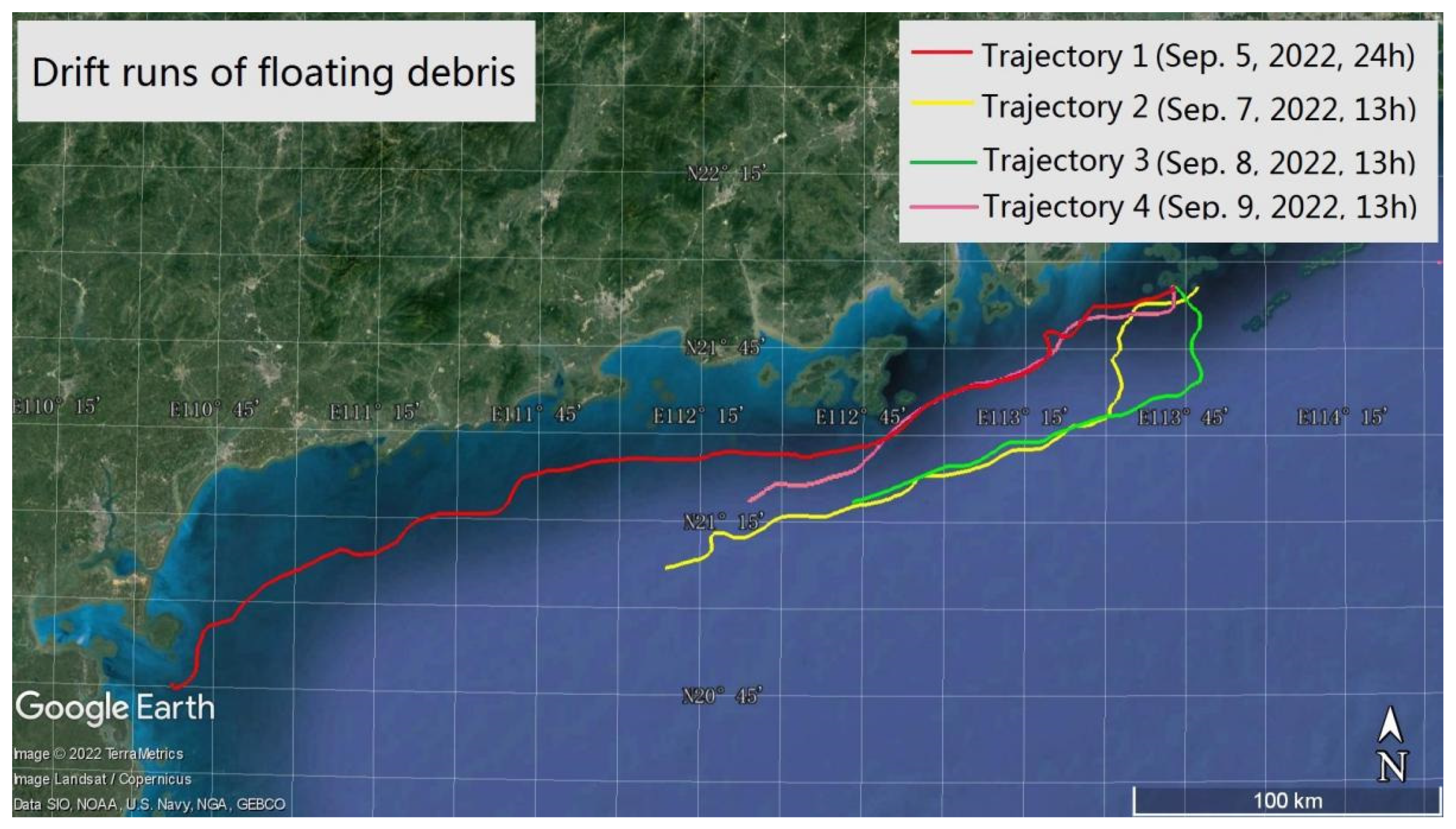
- To obtain a longer drift trajectory of the debris, the navigational observations are ceased, but the debris continues to drift, with its position data still being recorded. Simultaneously, coastal radars and marine weather stations continue to monitor the marine environment in the area of the sea trial where the debris is located. Eventually, four debris drift trajectories are obtained, as shown in Figure 4.
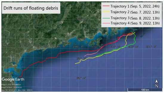 Figure 4. Drift trajectories from the debris drift experiment.
4. Results and Analysis
4.1. Analysis of Experimental Results
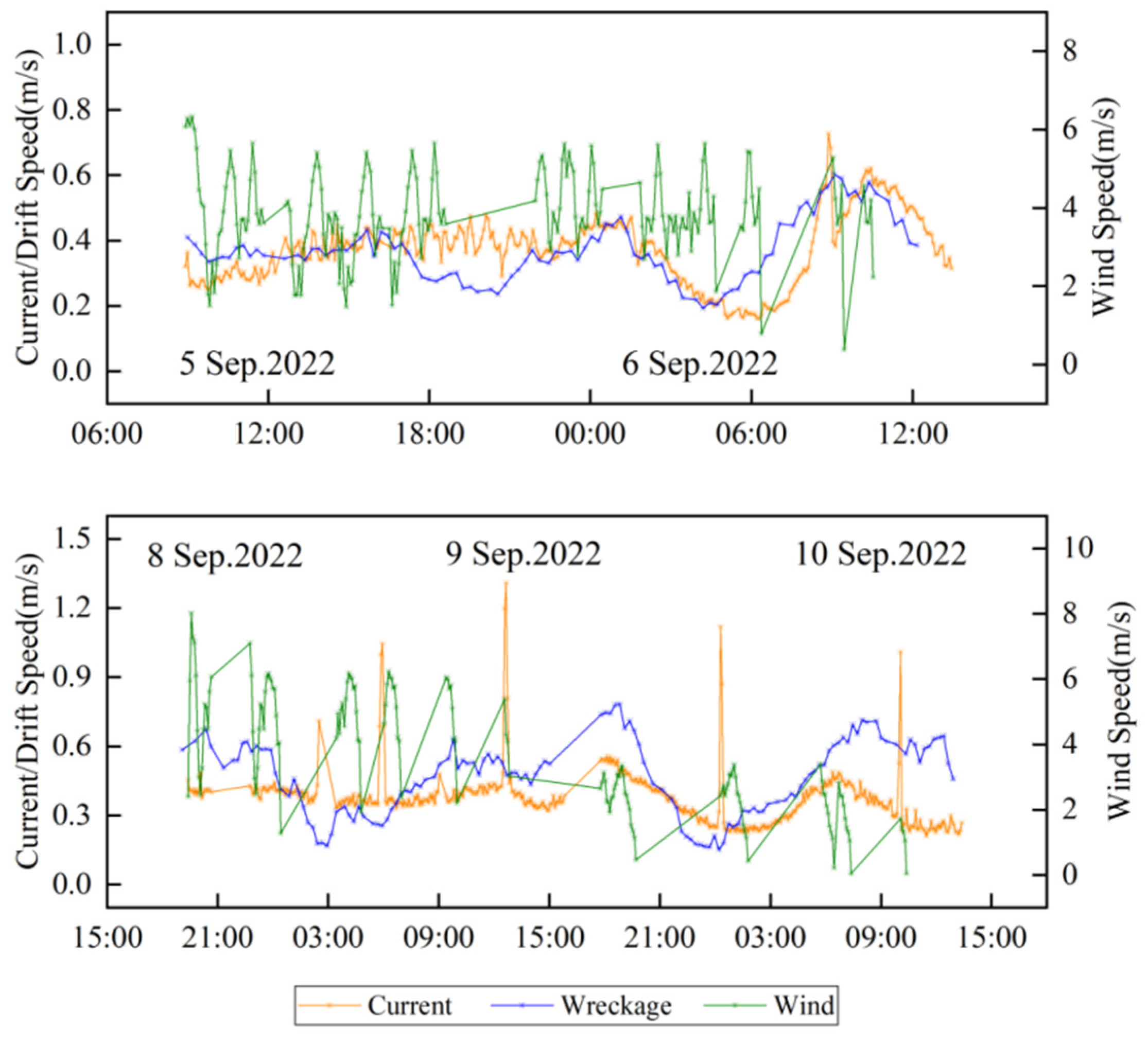
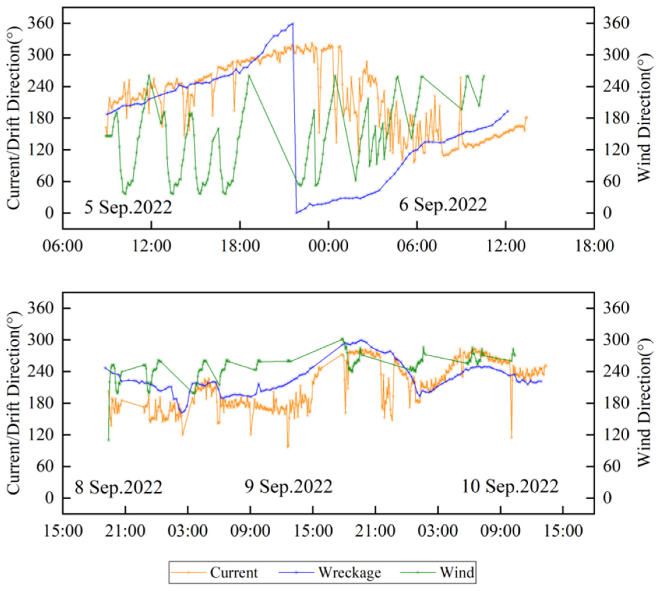
During the debris drift experiment, the variation over time in the drift speed of the debris, along with the concurrent sea current speed and wind speed, is illustrated in Figure 5. It is observed that the range of the current speed fluctuates between 0.2 and 0.6 m/s, showing relatively stable changes, while the wind speed varies more dramatically, ranging from 1.0–8.0 m/s. The drift speed of the debris varies between 0.2 and 0.7 m/s, generally aligning with the pattern of current speed changes. The experiment also analyzed the drift direction of the debris, along with the concurrent sea current and wind directions over time, as shown in Figure 6. The overall drift direction of the debris and the sea current is predominantly southwest, while the wind direction initially blows towards the southeast and later shifts to the southwest. It is also noted that when the current direction and the wind direction are not aligned, the drift speed of the debris is lower than the current speed; conversely, when they are aligned, the debris drift speed exceeds the current speed.
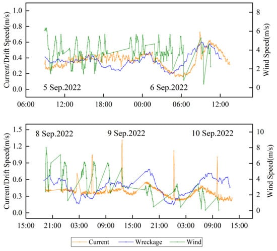
Figure 5.
Variation curves of debris drift speed, current speed, and wind speed over time.
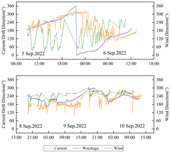
Figure 6.
Variation curves of debris drift direction, current direction, and wind direction over time.
Four effective trajectories were identified for the debris, and after decomposing the experimental data into 10-min averages, 393 valid samples were obtained. According to the change in the leeway direction, the numbers of positive and negative CWLs were tallied. Among these, the number of instances where the leeway drift vector of the debris veered right of the downwind direction was 186, accounting for 47.4% of cases. The instances of veering left of the downwind direction were 207, comprising 52.6% of cases, indicating that the probabilities of positive and negative CWLs are both close to 50%. The tracking buoy was used to record the drift track, velocity, and direction of debris in the drift experiment. The dynamics governing the CWL sign change, as the physical factors affecting the change may be numerous and subtle, and in general, were not directly measured during the leeway experiments. To further study the variations in the CWL direction, a statistical method was used to obtain the jibing frequency of the debris based on the drift sample data. The determination of downwind jibing events was based on relatively strict criteria, requiring the fulfillment of two conditions: (1) the CWL direction changes to the opposite side of the wind direction; (2) before and after the change, the CWL remains stable in the same direction for more than 20 min. Based on these criteria, the jibing frequency of the debris was found to be 7.7% per hour. The maximum leeway divergence angle was statistically determined to be 40.4°, representing the characteristic range of the leeway angle.
4.2. Calibration Results of Model Parameters
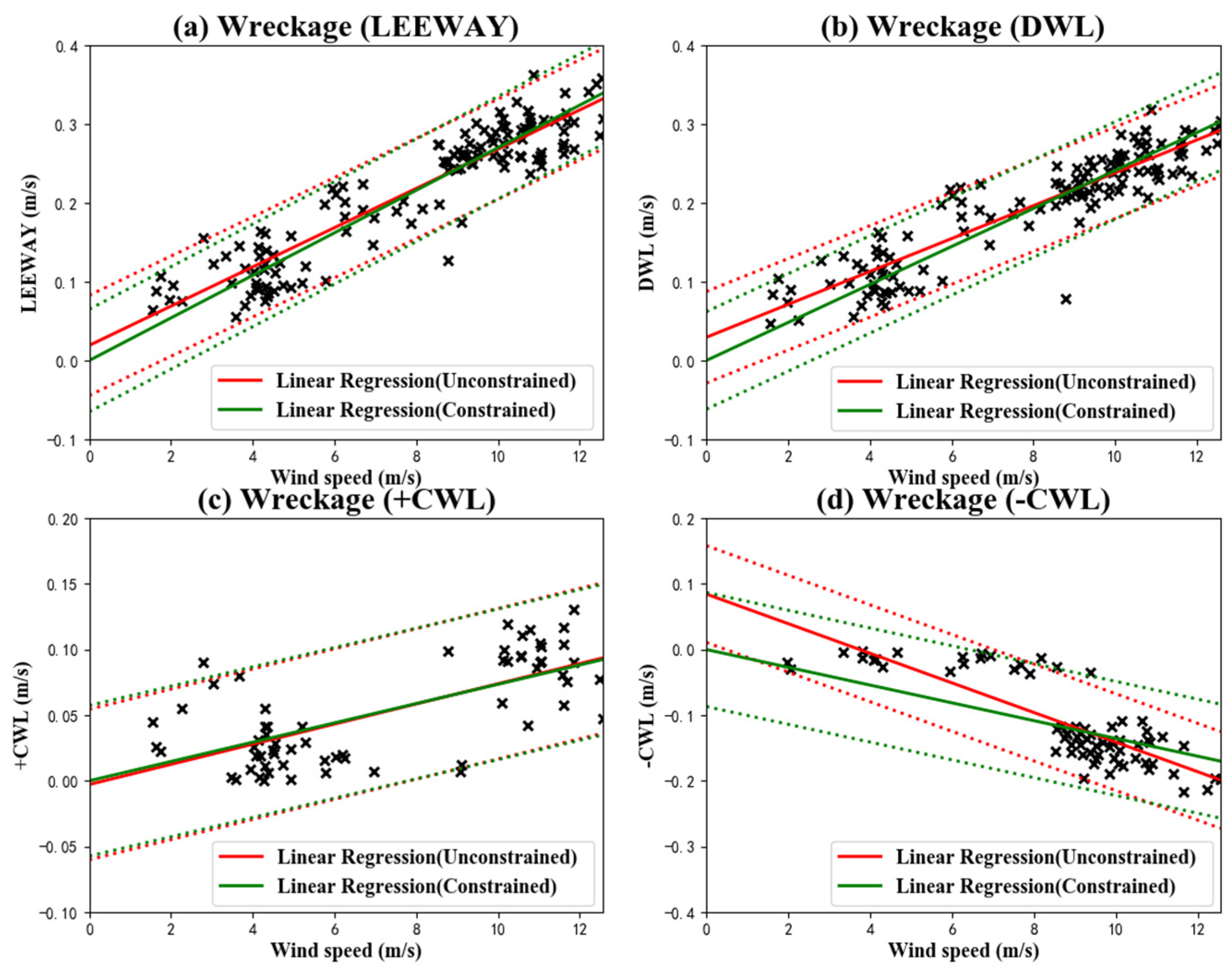
Before calibrating the parameters of the wind drift model, the initial task is to convert the start and end position coordinates of the debris within ten-minute sample intervals to calculate the debris’s drift velocity. After eliminating the influence of the current speed on the debris drift, the leeway velocity L and the wind deviation angle are obtained. From a vector decomposition of L, the DWL and CWL components are derived. Using the least squares method, linear fits are performed between the ten-meter wind speed and the DWL and CWL components, with their 95% confidence intervals being . The linear regression results of the debris wind drift model parameters are shown in Figure 7. The results indicate that both the DWL and CWL exhibit a strong linear relationship with the ten-meter wind speed. The corresponding calibration results of the model parameters are shown in Table 2. It is observed that, across all samples, the ten-meter wind speed ranged between 1.5 m/s and 13 m/s. The downwind, wind-induced drift speed DWL varied from 0 to 0.3 m/s, with a slope of 2.41% obtained from constrained linear regression and a fitting residual of 3.09 cm/s. In contrast, the slope from unconstrained regression was 2.09%, with an intercept of 2.94 cm/s and a fitting residual of 2.90 cm/s, indicating that the unconstrained regression results are more optimal. The right-deviating, crosswind-induced drift speed +CWL ranged from −0.03 to 0.13 m/s. The slope from the constrained linear regression was 0.74%, significantly lower than the fit slope between the DWL and ten-meter wind speed, with a fitting residual of 2.87 cm/s. The unconstrained regression yielded a slope of 0.77%, an intercept of −0.28 cm/s, and a fitting residual of 2.86 cm/s, again showing that unconstrained regression results are more optimal. The left-deviating, crosswind-induced drift speed −CWL varied from −0.25 to 0.05 m/s. The slope from the constrained linear regression was −1.36%, significantly lower than the fit slope between the DWL and ten-meter wind speed, with a fitting residual of 4.34 cm/s. The unconstrained regression produced a slope of −2.26%, an intercept of 8.45 cm/s, and a fitting residual of 3.69 cm/s, indicating that the unconstrained regression results are more optimal.
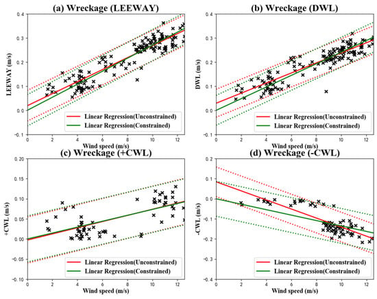
Figure 7.
Linear regression results in the AP98 model for the wind-induced drift velocity of debris (a), DWL component (b), +CWL component (c), and −CWL component (d) in relation to wind velocity at a height of ten meters. The red solid line represents the fit line with no constraints, the green solid line represents the constrained fit line, and the dashed lines indicate the 95% confidence interval range.

Table 2.
Calibration results of the AP98 model parameters for debris.
By substituting the results of the unconstrained linear regression back into the wind drift effect model, the relationship between the debris wind drift speed and the ten-meter wind speed can be established. The resulting debris AP98 wind drift effect model is as follows:
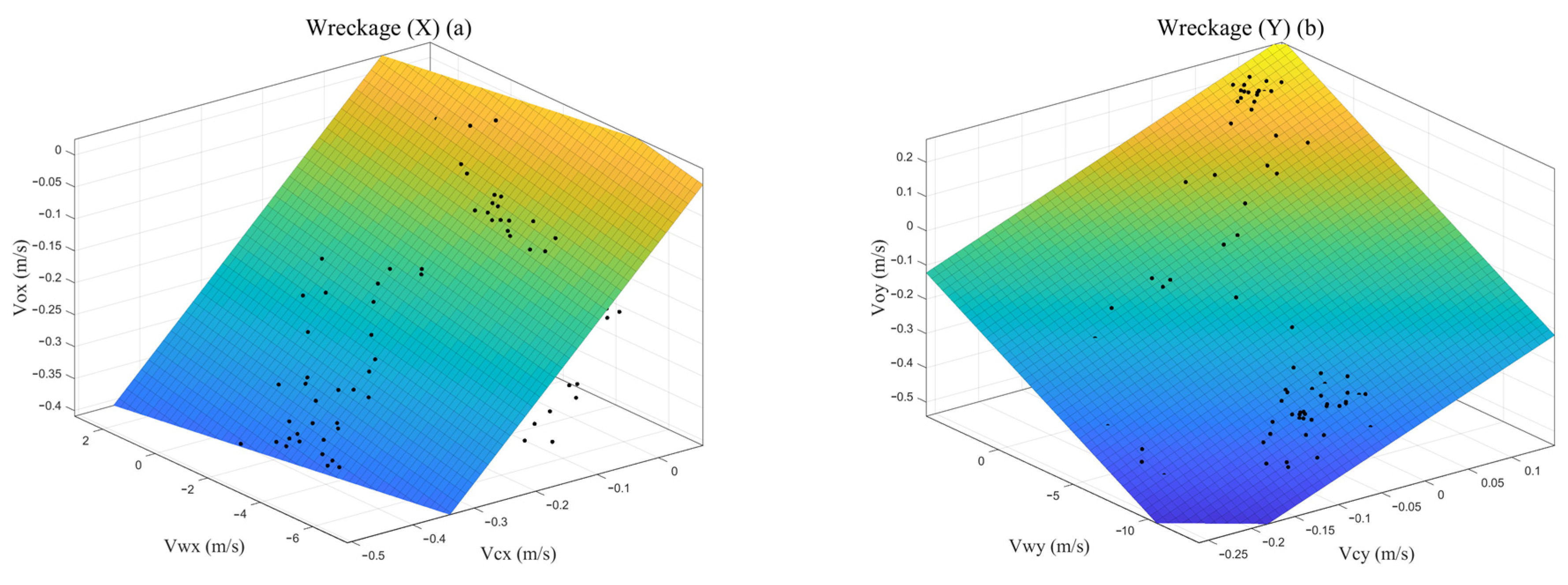
Based on the drift trajectories of maritime distress targets and synchronous observations of wind and currents, the parameters of the debris drift dynamics model were calibrated. The linear regression results of the model parameters are shown in Figure 8. It is observed that in all samples, on the east–west (X) axis, the drift speed of the debris is mostly negative, reaching up to about −0.4 m/s, corresponding to the 10 m high sea surface wind and sea water flowing westward. On the north–south (Y) axis, the debris drift speed, the 10 m high sea surface wind, and sea water are predominantly southward. On both axes, the debris drift speed shows a strong linear relationship with the 10 m high sea surface wind and sea surface current speed, exhibiting a good fit overall. The corresponding calibration results of the model parameters are shown in Table 3. In both the X and Y directions, the impact coefficients of the 10 m high sea surface wind are less than 0.03, while the impact coefficients of the sea surface current are more than 0.97, indicating that the influence of the sea surface current on the debris drift is much greater than that of the 10 m high sea surface wind. On the north–south (Y) axis, the RMSE (root mean square error) is about 0.038, more than half less than on the east–west (X) axis, suggesting a better fit on the north–south (Y) axis.
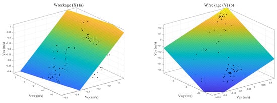
Figure 8.
Regression results of debris drift velocity in relation to the 10 m high sea surface wind speed and sea surface current speed (a) in the east–west (X) direction and (b) in the north–south (Y) direction.

Table 3.
Fitting parameters of the debris drift dynamics model.
Based on the calibration results of the parameters, the drift dynamics model for the debris is as follows:
Here, and represent the components of the debris drift velocity in the east–west and north–south directions, respectively. and are the components of the current speed in the east–west and north–south directions, respectively. Similarly, and correspond to the components of the wind speed in the east–west and north–south directions, respectively.
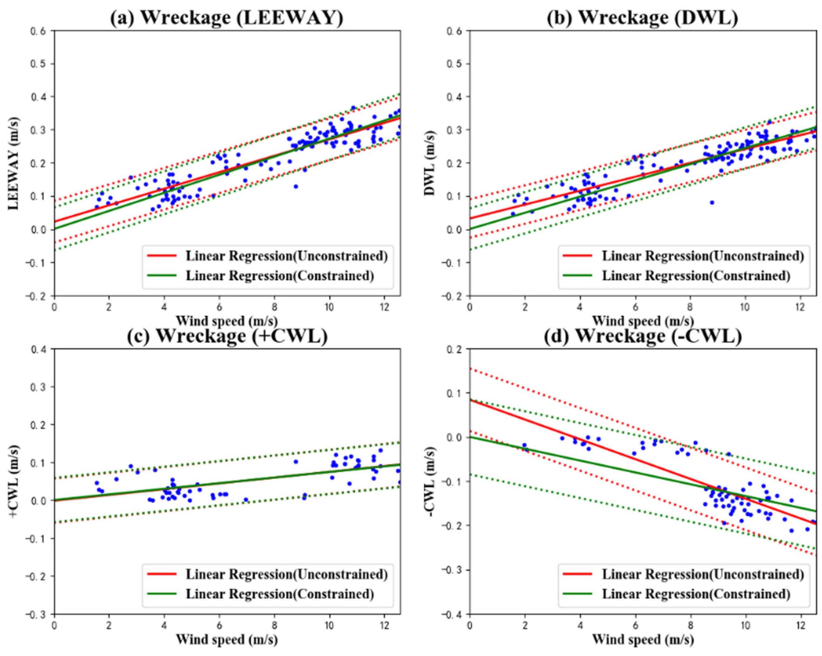
The parameters from the above-mentioned drift dynamics model are substituted into Equation (6) to calculate the new leeway velocity. Then, a least squares linear regression is adopted between this new leeway velocity and the wind speed. The linear regression of the debris leeway velocity, DWL, and CWL with respect to the ten-meter wind speed and their 95% confidence level statistics are shown in Figure 9. The results indicate that both the DWL and CWL have a strong linear relationship with the ten-meter wind speed. Similarly, the results from the unconstrained regression are more optimal than those from the constrained regression. The corresponding calibration results of the model parameters are presented in Table 4.
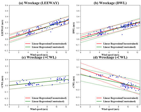
Figure 9.
Linear regression results in the improved model for the wind-induced drift velocity of debris (a), DWL component (b), +CWL component (c), and −CWL component (d) in relation to wind velocity at a height of ten meters. The red solid line represents the fit line with no constraints, the green solid line represents the constrained fit line, and the dashed lines indicate the 95% confidence interval range.

Table 4.
Calibration results of the improved model parameters for debris.
By substituting the results of the unconstrained linear regression back into the improved model, the formula for the improved debris model is as follows:
5. Comparison and Discussion
The Monte Carlo method is employed to simulate the drift trajectories of floating debris, so as to validate the effectiveness of the drift models. When simulating particle trajectories using the established drift prediction models, the probability of +CWL for the debris is set at 47.4%, and the probability of −CWL is set at 52.6%, based on the characteristics of the debris drift. Of 1000 random particles, 474 are used to simulate particle drift trajectories with +CWL, while the remaining 526 simulate trajectories with −CWL. Additionally, the frequency of debris jibing is set at 7.7% per hour. The calculation of particle drift trajectories uses Equations (8)–(10). Perturbations in the leeway coefficients of the particles are calculated using Equations (11)–(13).
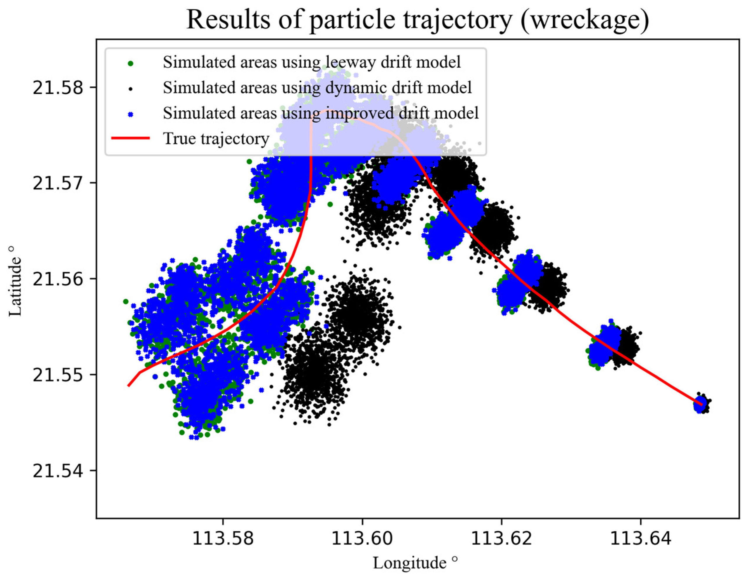
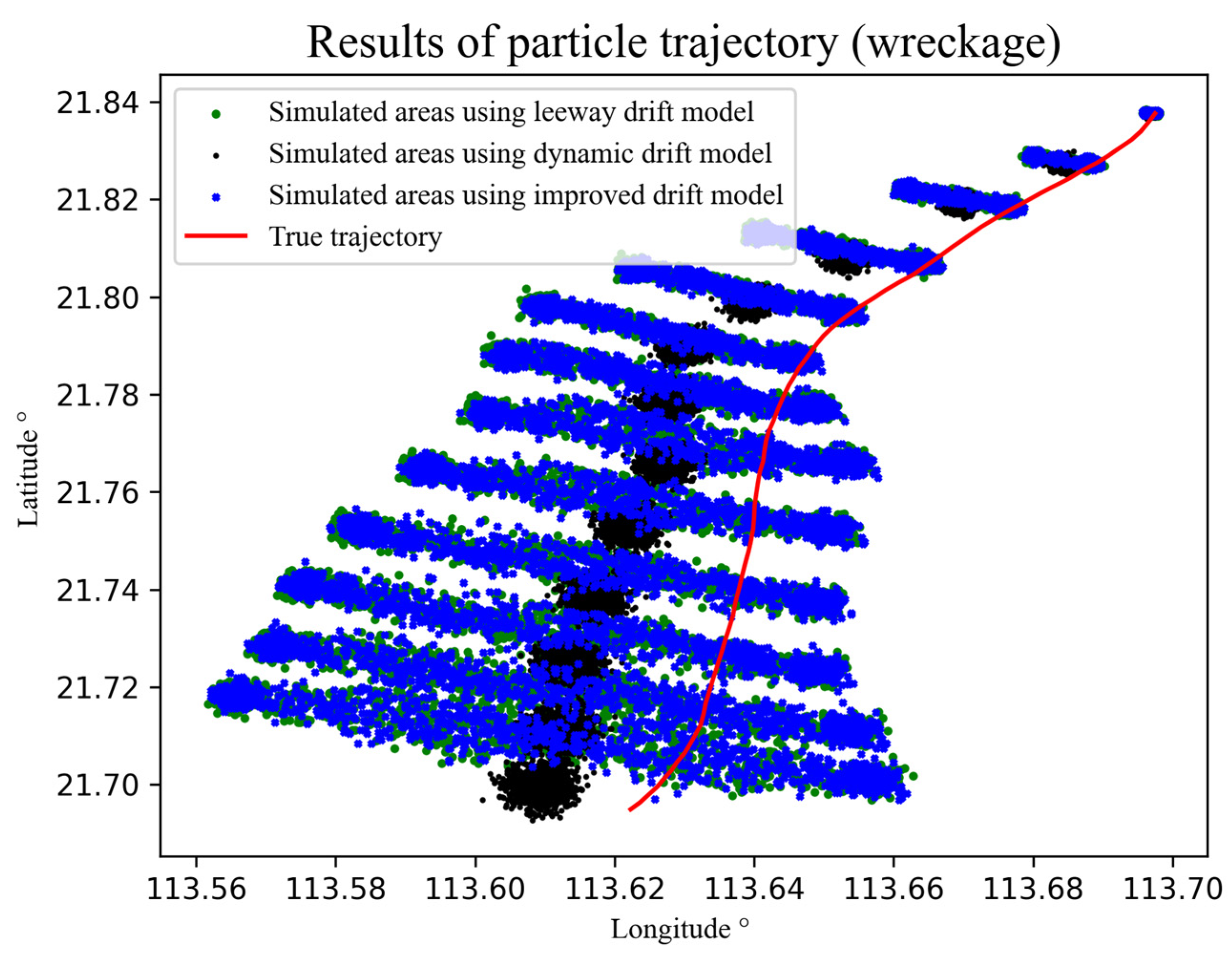
Two real trajectories from the debris drift experiment are selected for comparative analysis, corresponding to Case 1 and Case 2. The results of the Monte Carlo simulations for random particles in Case 1 are shown in Figure 10, and for Case 2, in Figure 11. The simulation results indicate that, in the AP98 leeway model and the improved model, due to the CWL direction being divided to the left and right sides of the wind speed, particles are distributed on both sides of the actual trajectory. In contrast, the particle trajectories simulated by the drift dynamics model always follow a single path. Moreover, with the passage of time, the simulation error and the search area gradually increase. The average hourly deviation between the simulated random particles and the actual trajectory in Case 1, as well as the final average deviation, are presented in Table 5. After 10 h, the average drift deviation for the debris in the AP98 model was 0.46 km, in the dynamic model, was 0.68 km, and in the improved model, was 0.44 km. The improved model outperformed both the AP98 leeway model and the dynamic model in simulating debris drift. The average hourly deviation between the simulated random particles and the actual trajectory in Case 2, as well as the final average deviation, are presented in Table 6. After 10 h, the average drift deviation for the debris in the AP98 model was 1.72 km, in the dynamic model, was 1.91 km, and in the improved model, was 1.64 km. The improved model also showed a superior performance in simulating debris drift in Case 2 compared to the AP98 leeway model and the dynamic model. Combining the simulation results of the two models in both Case 1 and Case 2, it is observed that the improved model’s accuracy in simulating debris drift is higher than those of the AP98 leeway model and the dynamic model.
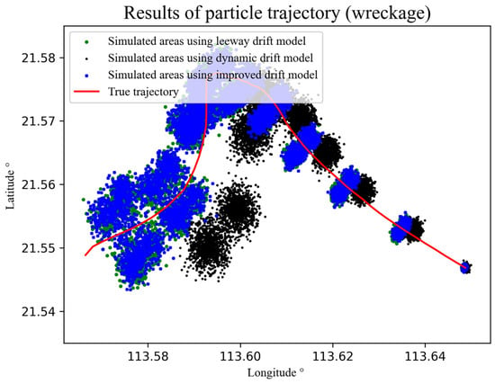
Figure 10.
The trajectory simulation results of the Monte Carlo simulations for random particles in Case 1 (the true trajectory is plotted in red, the simulation results of the leeway drift model are plotted in green, the simulation results of the dynamics drift model are plotted in black, and the simulation results of the improved drift mode are plotted in blue).
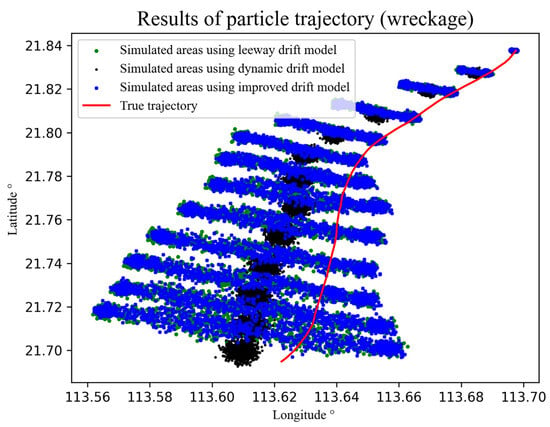
Figure 11.
The trajectory simulation results of the Monte Carlo simulations for random particles in Case 2 (the true trajectory is plotted in red, the simulation results of the leeway drift model are plotted in green, the simulation results of the dynamics drift model are plotted in black, the simulation results of the improved drift mode are plotted in blue).

Table 5.
The average distance error (km) between the simulated trajectories and the true trajectory in Case 1.

Table 6.
The average distance error (km) between the simulated trajectories and the true trajectory in Case 2.
6. Conclusions
In this paper, a series of drift experiments were carried out in the South China Sea to study the drift characteristics and drift models of floating debris. Some drift characteristics of the debris were obtained. The probability of positive crosswind leeway (CWL) was 47.4%, while the probability of negative crosswind leeway (CWL) was 52.6%. The jibing frequency was 7.7% per hour, and the maximum leeway divergence angle was 40.4 degrees. Based on extensive experimental data, nine coefficients for the debris’s AP98 model, four coefficients for the dynamics model, and nine coefficients for the improved model were determined using the least squares method. For the AP98 model, the downwind slope, intercept, and standard error were 2.09%, 2.94 cm/s, and 2.90 m/s, respectively, while the coefficients for right- and left-side winds were: 0.77%, −0.28 cm/s, and 2.86 cm/s and −2.26%, 8.45 cm/s, and 3.69 cm/s. The coefficients for the drift dynamics model were divided into the X and Y directions, with the λ_X at 99.01% and the λ_Y at 97.28%. The improved model’s downwind slope, intercept, and standard error were 2.09%, 3.71 cm/s, and 2.90 cm/s, respectively, and the coefficients for the right- and left-side winds were 0.76%, −0.18 cm/s, and 2.92 cm/s and −2.24%, 8.41 cm/s, and 3.53 cm/s. Three types of marine debris drift prediction models were finally established. The Monte Carlo technique was used to evaluate these three drift prediction models, finding that the improved model’s predictive accuracy was higher than that of the AP98 leeway model and the dynamic model. Overall, the three debris drift prediction models established in this paper can be directly used to guide the search for floating debris in the South China Sea.
Author Contributions
Conceptualization, H.T.; methodology, L.M., H.T. and F.Q.; software, S.J.; validation, X.G. and Z.C. (Zhihui Chen); formal analysis, T.Z.; investigation, R.Z.; resources, X.G. and Z.C. (Zhi Chen); data curation, Z.C. (Zhihui Chen) and R.Z.; writing—original draft preparation, L.M. and H.T.; writing—review and editing, F.Q., T.Z. and Z.C. (Zhi Chen); visualization, S.J.; supervision, H.T.; project administration, L.M.; funding acquisition, L.M. All authors have read and agreed to the published version of the manuscript.
Funding
This work was supported by the National Key Research and Development Program of China (grant No. 2021YFC3101800), National Natural Science Foundation of China (grant No. U2006210), and Shenzhen Science and Technology Program (grant No. KCXFZ20211020164015024).
Institutional Review Board Statement
Not applicable.
Informed Consent Statement
Not applicable.
Data Availability Statement
The raw data supporting the conclusions of this article will be madeavailable by the authors upon request.
Conflicts of Interest
The authors declare no conflicts of interest.
References
- Safety Investigation Team for MH370: Factual Information–Safety Investigation for MH370; Tech. Rep. MH370/01/15; Ministry of Transport: Putrajaya, Malaysia, 2015.
- ATSB: MH370—Definition of Underwater Search Areas; Tech. Rep. AE-2014-054; Australian Transportation Safety Bureau: Canberra, Australia, 2015.
- Jansen, E.; Coppini, G.; Pinardi, N. Drift simulation of MH370 debris using superensemble techniques. Nat. Hazards Earth Syst. Sci. 2016, 16, 1623–1628. [Google Scholar] [CrossRef]
- Huang, G.; Law, A.W.K.; Huang, Z. Wave-induced drift of small floating objects in regular waves. Ocean Eng. 2011, 38, 712–718. [Google Scholar] [CrossRef]
- Chen, C.; Shiotani, S.; Sasa, K. Effect of ocean currents on ship navigation in the east China sea. Ocean Eng. 2015, 104, 283–293. [Google Scholar] [CrossRef]
- Cucco, A.; Quattrocchi, G.; Satta, A.; Antognarelli, F.; De Biasio, F.; Cadau, E.; Umgiesser, G.; Zecchetto, S. Predictability of wind-induced sea surface transport in coastal areas. J. Geophys. Res. Oceans 2016, 121, 5847–5871. [Google Scholar] [CrossRef]
- Ličer, M.; Estival, S.; Reyes-Suarez, C.; Deponte, D.; Fettich, A. Lagrangian modelling of a person lost at sea during the Adriatic scirocco storm of 29 October 2018. Nat. Hazards Earth Syst. Sci. 2020, 20, 2335–2349. [Google Scholar] [CrossRef]
- Anderson, E.; Odulo, A.; Spaulding, M. Modeling of Leeway Drift; U.S. Coast Guard Research and Development Center: New London, CT, USA, 1998. [Google Scholar]
- Kubota, M. A Mechanism for the Accumulation of Floating Marine Debris North of Hawaii. J. Phys. Oceanogr. 1994, 24, 1059–1064. [Google Scholar] [CrossRef]
- Martinez, E.; Maamaatuaiahutapu, K.; Taillandier, V. Floating marine debris surface drift: Convergence and accumulation toward the South Pacific subtropical gyre. Mar. Pollut. Bull. 2009, 58, 1347–1355. [Google Scholar] [CrossRef] [PubMed]
- Dobler, D.; Huck, T.; Maes, C.; Grima, N.; Blanke, B.; Martinez, E.; Ardhuin, F. Large impact of Stokes drift on the fate of surface floating debris in the South Indian Basin. Mar. Pollut. Bull. 2019, 148, 202–209. [Google Scholar] [CrossRef] [PubMed]
- Maximenko, N.; Hafner, J.; Kamachi, M.; MacFadyen, A. Numerical simulations of debris drift from the Great Japan Tsunami of 2011 and their verification with observational reports. Mar. Pollut. Bull. 2018, 132, 5–25. [Google Scholar] [CrossRef] [PubMed]
- Gao, J.; Mu, L.; Wang, G.; Li, C.; Dong, J.; Bao, X.; Li, H.; Song, J. Drift analysis and prediction of debris from Malaysia Airlines flight MH370. Chin. Sci. Bull. 2016, 61, 2409–2418. [Google Scholar] [CrossRef]
- Durgadoo, J.V.; Biastoch, A.; New, A.L.; Rühs, S.; Nurser, A.J.G.; Drillet, Y.; Bidlot, J. Strategies for simulating the drift of marine debris. J. Oper. Oceanogr. 2021, 14, 1–12. [Google Scholar] [CrossRef]
- Allen, A.A.; Plourde, J.V. Review of Leeway: Field Experiments and Implementation (No. CG-D-08-99); Coast Guard Research and Development Center Groton CT: New London, CT, USA, 1999. [Google Scholar]
- Allen, A.A. Leeway Divergence (No. CG-D-05-05); Coast Guard Research and Development Center Groton CT: New London, CT, USA, 2005. [Google Scholar]
- Allen, A.; Roth, J.; Maisondieu, C.; Breivik, Ø.; Forest, B. Field Determination of the Leeway of Drifting Objects; Tech. Rep. 17/2010; Norwegian Meteorological Institute: Oslo, Norway, 2010. [Google Scholar]
- Breivik, Ø.; Allen, A.A. An operational search and rescue model for the Norwegian Sea and the North Sea. J. Mar. Syst. 2008, 69, 99–113. [Google Scholar] [CrossRef]
- Breivik, Ø.; Allen, A.A.; Maisondieu, C.; Roth, J.C. Wind-induced drift of objects at sea: The leeway field method. Appl. Ocean Res. 2011, 33, 100–109. [Google Scholar] [CrossRef]
- Breivik, Ø.; Allen, A.A.; Maisondieu, C.; Roth, J.; Forest, B. The leeway of shipping containers at different immersion levels. Ocean Dynam. 2012, 62, 741–752. [Google Scholar] [CrossRef]
- Breivik, Y.; Allen, A.A.; Maisondieu, C.; Olagnon, M. Advances in search and rescue at sea. Ocean Dynam. 2013, 63, 83–88. [Google Scholar] [CrossRef]
- Brushett, B.A.; Allen, A.A.; Futch, V.C.; King, B.A.; Lemckert, C.J. Determining the leeway drift characteristics of tropical Pacifc island craft. Appl. Ocean Res. 2014, 44, 92–101. [Google Scholar] [CrossRef]
- Zhu, K.; Mu, L.; Tu, H. Exploration of the wind-induced drift characteristics of typical Chinese offshore fishing vessels. Appl. Ocean Res. 2019, 92, 101916. [Google Scholar] [CrossRef]
- Tu, H.; Wang, X.; Mu, L.; Xia, K. Predicting drift characteristics of persons-in-the-water in the South China Sea. Ocean Eng. 2021, 242, 110134. [Google Scholar] [CrossRef]
- Zhang, J.; Teixeira, Â.P.; Guedes Soares, C.; Yan, X. Probabilistic modelling of the drifting trajectory of an object under the effect of wind and current for maritime search and rescue. Ocean Eng. 2017, 129, 253–264. [Google Scholar] [CrossRef]
- Melsom, A.; Counillon, F.; LaCasce, J.H.; Bertino, L. Forecasting search areas using ensemble ocean circulation modeling. Ocean Dynam. 2012, 62, 1245–1257. [Google Scholar] [CrossRef]
Disclaimer/Publisher’s Note: The statements, opinions and data contained in all publications are solely those of the individual author(s) and contributor(s) and not of MDPI and/or the editor(s). MDPI and/or the editor(s) disclaim responsibility for any injury to people or property resulting from any ideas, methods, instructions or products referred to in the content. |
© 2024 by the authors. Licensee MDPI, Basel, Switzerland. This article is an open access article distributed under the terms and conditions of the Creative Commons Attribution (CC BY) license (https://creativecommons.org/licenses/by/4.0/).

