Hydrodynamic Modeling of a Large, Shallow Estuary

Abstract

Florida Bay, a large and shallow estuary, serves as a vital habitat for a diverse range of marine species and holds significant environmental, commercial, and recreational value. The Florida Bay ecosystem is under extensive stress due to decades of increased nutrient loads. Based on the Environmental Fluid Dynamics Code (EFDC), a hydrodynamic model was developed in this study. The model was calibrated with a comprehensive dataset, including measurements over 7 years from 34 tidal stations, 42 current stations, and 14 temperature and salinity stations. Key findings include the following: (1) the bay exhibits a shift in the tidal regime, transitioning from macro-tidal in the western region to micro-tidal in the central and eastern/northeast regions; (2) local winds and the subtidal variations from the coastal ocean are the primary drivers for the hydrodynamic processes in the eastern and central regions; (3) salinity changes in the bay are primarily controlled by three processes: the net supply of freshwater, the processes that drive mixing within the estuary (e.g., wind, topography, currents), and the exchange of salinity with the coastal ocean. This hydrodynamic model is essential for providing a comprehensive tool to address environmental challenges and sustain the bay’s ecosystem health.

1. Introduction

The hydrodynamic modeling of estuaries has a long history [1]. The past decade has witnessed a significant surge in the complexity and capabilities of estuarine hydrodynamic modeling. Driven by progress in computational power, numerical algorithms, and data-acquisition techniques, researchers have pushed the boundaries of understanding estuarine processes. For example, Ganju et al. [2] provided a comprehensive overview of the evolution of estuarine modeling, discussing progress in terms of both hydrodynamic and ecological aspects, along with remaining challenges. Iglesias et al. [3] highlighted the growing use of model ensembles for capturing uncertainties in climate change projections and their impacts on estuarine hydrodynamics. Iglesias et al. [4] showcased the application of a high-resolution model to capture complex flow patterns in a shallow estuary, including stratification and eddies. Hein et al. [5] focused on the use of a sophisticated model to analyze tidal resonances and their impact on mixing and transport in a semi-closed estuary. Zhang et al. [6] simulated storm surges in an estuary and tidal wetlands caused by several typhoons.

Florida Bay is a triangular estuary, bordered to the north and east by the southern mainland of the Florida peninsula and to the south by the Florida Keys and opening into the Gulf of Mexico on the west (Figure 1). The bay is large and shallow, covering around 2200 square kilometers (km), with depths averaging less than one meter (m) [7]. About 80% of the estuary falls within the Everglades National Park (ENP), and much of the remaining portion lies within the Florida Keys National Marine Sanctuary. Florida Bay holds economic importance as a tourist, commercial fishing, and recreational area. Shallow and often hyper-saline, the bay was, until recently, known for clear waters and lush seagrass meadows covering a mosaic of shallow water banks and numerous relatively deeper water basins. It provides essential habitat for numerous marine species with environmental, commercial, and recreational importance.

A defining feature of the bay is its shallow depth. Light sufficient to support photosynthesis can reach the sediment surface in almost all areas of the bay, resulting in the dominance of seagrass beds as both a habitat and a source of primary production. The shallowness of the bay also affects its circulation and salinity regime. Florida Bay includes over 200 small islands or “keys”. Its complex network of shallow mud banks restricts horizontal water exchange among the bay’s basins and between these basins and the Gulf of Mexico. The net freshwater supply in Florida Bay is the sum of rainfall over the area plus the inflow of freshwater through the coastal mangroves from the Everglades minus evaporation. Rainfall and evaporation dominate the freshwater budget in Florida Bay, but inflow from the Everglades is comparable in magnitude to the difference between rainfall and evaporation. The salinity of Florida Bay can rise rapidly during drought periods due to the excess of evaporation and the lack of precipitation and/or freshwater inflow. In recent decades, Florida Bay has behaved as a marine lagoon, with salinities as high as 70 ppt reported in central Florida Bay. During drought years, salinity typically exceeded 40 ppt over most of the bay [8,9].

Estuaries and shallow coastal waters around the world have been heavily affected by human activities in the past decades [8,10]. Florida Bay is an example. The encroachment of people and their desire to live near the water has placed a great deal of stress on this shallow water system. The Florida Bay ecosystem is currently under extensive stress due to decades of increased nutrient loads along its northern boundary. Although the nutrient loading along the northern boundary has increased, the net freshwater inflow has decreased due to the large-scale anthropogenic diversion of much of the natural southward flow through the Everglades to the southeast coast of the Florida mainland. Consequently, the water quality in Florida Bay has been deteriorating for many years, as indicated by the increase in the size and persistence of algal blooms, die-off in seagrass beds, storm-event damage, and other water quality conditions throughout the bay. The cause of these water quality problems is further complicated by the lack of freshwater inflow and poor circulation patterns [8]. Reversing ecosystem decline and the re-establishment of a healthy stable ecosystem in Florida Bay is one of the major objectives of the Comprehensive Everglades Restoration Plan (CERP). CERP is one of the largest and most expensive restoration efforts in the world [11,12,13].

Mathematical models are widely accepted as providing the means to project water quality response and ecological impacts under different management scenarios. A key advantage of modeling is the ability to delineate the cause-and-effect relationships between pollutant sources and the resultant water quality, allowing the environmental manager to identify and target needed pollutant source controls by location and magnitude. The development and application of a coupled hydrodynamic and water quality modeling system for Florida Bay is essential in the scientific identification of cause-and-effect relationships between freshwater inflow, nutrient loading, and ecosystem health. A previous study modeling the water quality of Florida Bay was constrained due to limitations of the hydrodynamics used to provide physical transport [14,15]. Other studies associated with Florida Bay include modeling efforts by Wang et al. [16], Wang [17], and Sheng et al. [18].

The objective of this study is to develop a hydrodynamic model to simulate the bay under a wide range of freshwater inflow and climatic conditions. The development of a water quality model of Florida Bay will be presented in a separate paper. The Florida Bay Model (FBM) will be calibrated using a comprehensive dataset over a 7-year period. The calibrated FBM will then be applied to simulate hydrodynamic processes in Florida Bay and to investigate some key topics in estuarine modeling, including the impacts of tides, local winds, open boundary conditions, and model grid resolution.

2. Model Setup

The FBM is developed under the framework of the Environmental Fluid Dynamics Code (EFDC), a public-domain modeling package for simulating three-dimensional flow, transport, and biogeochemical processes in surface water systems [19,20]. This model solves the three-dimensional, vertically hydrostatic, free surface, turbulent averaged equations of motions for a variable density fluid. Dynamically coupled transport equations for turbulent kinetic energy, turbulent length scale, and temperature are also solved. The two turbulence transport equations implement the Mellor Yamada level 2.5 turbulence closure scheme [21,22]. Applications of the EFDC model include the wetting and drying simulation of Morro Bay, California [23], modeling sediment and metals transport in Blackstone River, Massachusetts [24], simulations of Lake Okeechobee hydrodynamic, thermal, sediment, and water quality processes (e.g., [25]), coupled hydrodynamic and water quality modeling of St. Lucie Estuary (e.g., [26]), and wetland modeling (e.g., [27]). Ji [1] provides detailed discussions of the EFDC model, its applications, and estuarine modeling.

The modeling period covers seven years, with an extensive set of measured data for model calibration, including 34 tidal stations, 42 tidal current stations, and 14 temperature and salinity stations.

2.1. Model Grid

Two versions of the model grid are generated (Figure 2): one includes the northeast wetland, and the other is truncated at the nominal coastline in the northeast region. Figure 2a displays the entire model grid, Figure 2b provides a blow-up of the model grid with the northeast wetland, and Figure 2c shows the blow-up of the model grid truncated at the nominal coastline in the northeast region. The model grid with the northeast wetland consists of 4300 grid cells in the horizontal direction, with cell size varying from approximately 500 m in the eastern interior of the bay to approximately 8 km at the western open boundary in the Gulf of Mexico. The model has two sigma vertical layers. Sensitivity tests on model grid resolution will be presented in Section 4.2.

Florida Bay is a complex combination of shallow bays, keys, bars, cuts, and narrows. The interior region of Florida Bay is characterized by shallow open-water sub-basins separated by narrow shoals or ridges and large, extremely shallow regions that may become exposed during periods of low sea level. Its bathymetry and topography data are based on the United States Geological Survey (USGS) bathymetric and topographic surveys of Florida Bay and the adjacent wetlands of the ENP and the southwest Florida coast, the National Oceanic and Atmospheric Administration (NOAA) Coastal Relief bathymetry, and NOAA soundings [28,29]. In areas with no observed data, primarily corresponding to banks in the bay, thematic mapping-based elevation data were also incorporated into the data model. In regions with unknown or poorly known bathymetry, the bottom elevations are set to 0.3 m. This default bottom elevation of banks and shoals is primarily based on the reported inability of USGS survey vessels to take bathymetric measurements in regions with water depths less than approximately 0.3 m [24]. 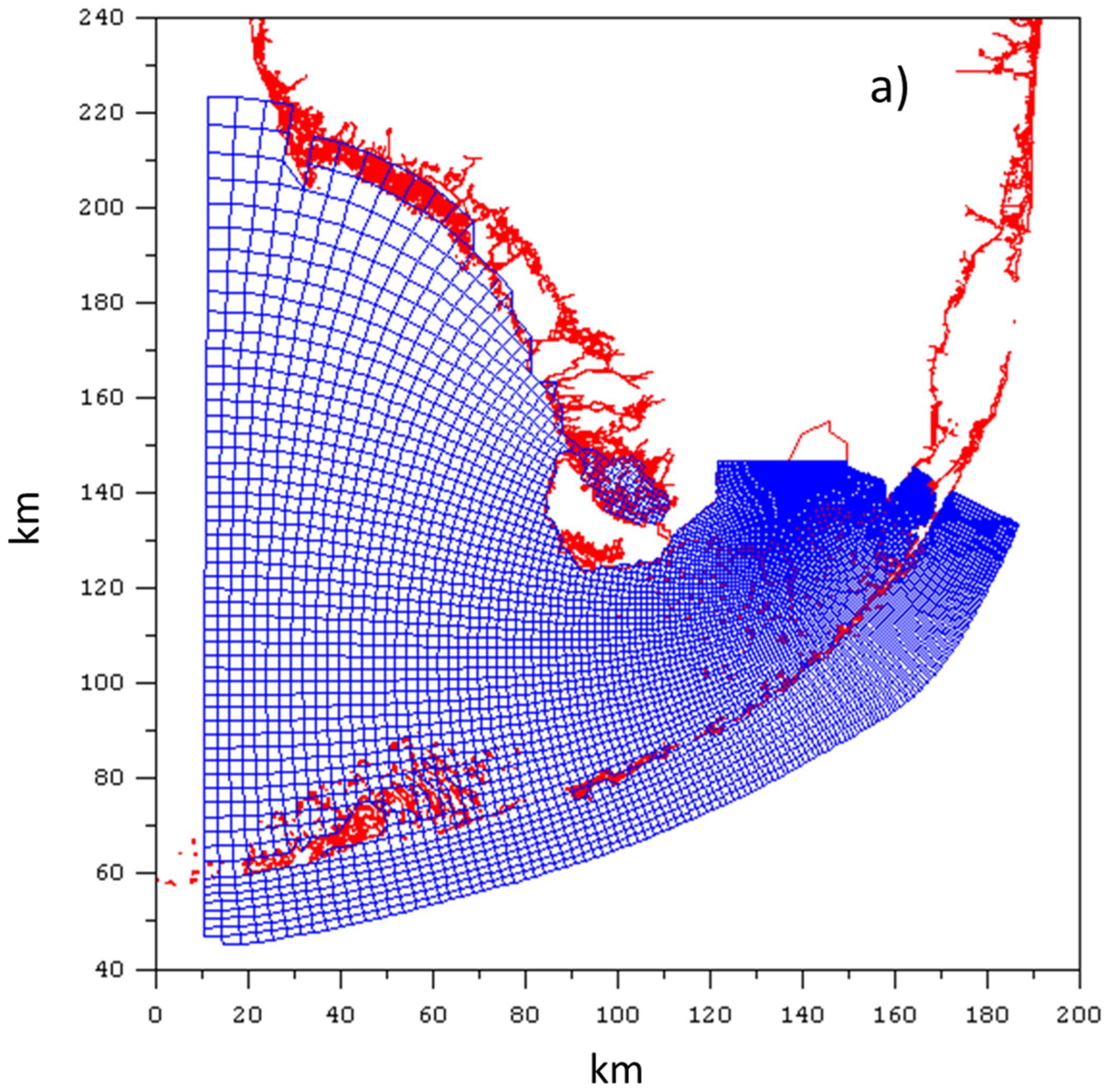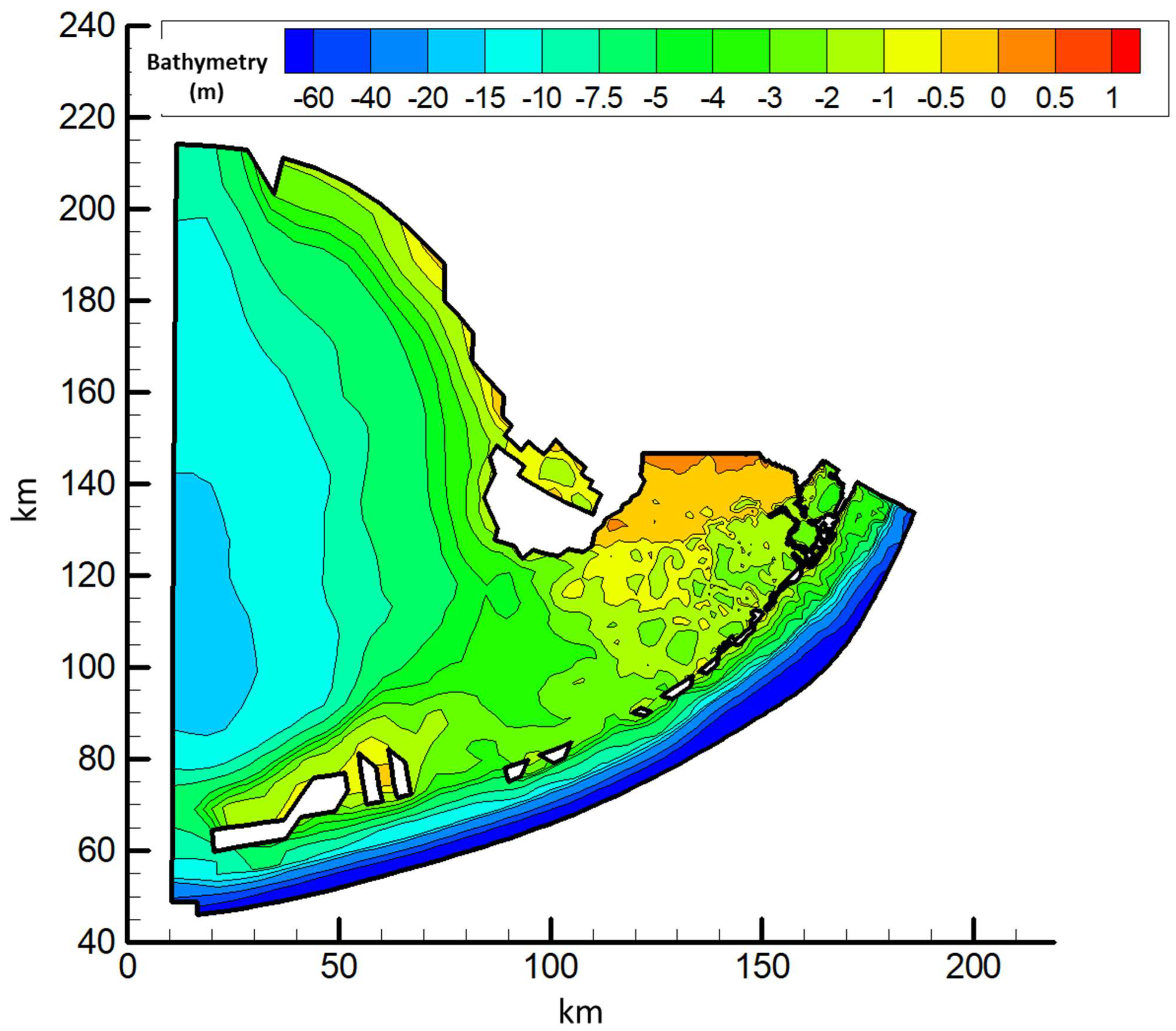Figure 3 presents the bathymetry and topography interpolated to the model grid.

2.2. External Forcings

Florida Bay is forced hydrodynamically by tides, winds, density currents, and other forcings. The hydrodynamic model was configured for a 7-year simulation period, spanning from 1 January 1996 through 31 December 2002. An additional year of model spin-up corresponding to 1995 was included, extending the total simulation period to eight years. Actual data to construct forcing functions were available for 1995, except for fresh and brackish water inflow. Inflows for 1999 were used for 1995 based on the hydrological similarity between 1999 and 1995.

Circulation in Florida Bay is forced by water surface elevation and transport along the western boundary with the Gulf of Mexico and the southern boundary in the Florida Straits. The hydrodynamic boundary condition along these open boundaries is a radiation-separation condition, expressed as:

$$\zeta -\frac{\mathbf{n}·\mathbf{u}H}{\sqrt{gH}}=2{\zeta }_R$$

(1)

where ζ is the water surface elevation relative to sea level, n is the outward normal vector to the boundary, u is the horizontal barotropic velocity vector, H is the water depth, ζ_R is the equivalent progressive wave amplitude, and g is the gravitational constant. The water surface elevation along the open boundaries consists of periodic tidal components and a transient or low-frequency component in the subtidal frequency spectrum. The equivalent incoming wave boundary condition (1) was specified as the sum of a low frequency component and harmonic components:

$${\zeta }_R={\zeta }_{LF}+{\displaystyle \sum _{m=1}^M\left({\zeta }_{RCm}\cos \left({\omega }_{m}t\right)+{\zeta }_{RSm}\sin \left({\omega }_{m}t\right)\right)}$$

(2)

where ζ_LF is the low-frequency water surface elevation, M is the number of tidal constituents, ζ_RCm and ζ_RSm are cosine and sine amplitudes at frequency ω_m, and t is time. Five harmonic constituents (M₂, S₂, N₂, K₁, and O₁) were used. The locations of 34 tidal gauge stations are shown in Figure 4a. Tidal gauge information is sparse along the open boundary, requiring the estimation of tidal frequency components of the incoming wave open boundary condition through an inverse procedure described by Tetra Tech [23].

Salinity and temperature open boundary conditions were specified in a spatially varying manner along the open boundaries using monitoring data from Florida International University [23].

Wind forcing was provided by wind records at five C-Man or National Data Buoy Center overwater stations [28]. Wind speed and direction in each model cell were determined as an inverse square distance-weighted average of the five stations. Atmospheric data included air temperature, relative humidity, rainfall, solar radiation, and cloud cover. Air temperature, relative humidity, and cloud cover were based on National Weather Service (NWS) data at Key West, Naples, Marathon, and Miami. Solar radiation was estimated from theoretical clean sky values and cloud cover, adjusted by comparison with the actual solar radiation data from a South Florida Water Management District (SFWMD) station. Rainfall data at the NWS stations were supplemented by ENP rainfall data. The final atmospheric datasets were spatially located at the four NWS stations, and values in each model cell were determined as an inverse squares distance-weighted average of the four stations [28].

The primary sources of freshwater entering the bay include distinct creeks and rivers along the coastline of Florida mainland and direct rainfall (Figure 1). Inflows from the creeks and rivers can range seasonally from fresh to brackish, depending on net freshwater flow southward from the Everglades, the extent of saltwater intrusion into the mangrove regions, and the low-frequency sea-level change in the bay driven primarily by sea levels to the west and south in the Gulf of Mexico and the Florida Straits. Other less quantified fresh and brackish water sources to the bay include distributed surface and groundwater flow along the northern boundary and, to a lesser extent, runoff from the keys.

Fresh and brackish water inflow along the boundaries of the model domain is provided by the USGS TIME model [30]. The TIME model provides an estimate of net freshwater inflow at 12 locations along the nominal coastline of Florida Bay. For model simulations using the nominal coastline version of the grid (as shown in Figure 2c), the 12 freshwater inflows were used and assigned zero inflowing salinity. For model simulations using the northeast wetland version of the grid (as shown in Figure 2a,b), brackish inflows were assigned to the model cells, which were assigned upwind salinities from the TIME simulation.

3. Hydrodynamic Model Calibration

Model calibration involves adjusting model parameter values within reasonable and acceptable ranges to minimize deviations between model results and measured data, ensuring accuracy within acceptable ranges. Hydrodynamic model calibration entails adjusting open boundary forcing, bottom roughness, and bottom elevations to achieve the best agreement between model simulations and observations of water surface elevation, currents, water temperature, and salinity.

The bottom roughness in the Western Gulf region and the Southern Florida Straits region was fine-tuned to a log law roughness height of 1.5 cm based on achieving fits of tidal water surface elevations along the western boundary of Florida Bay and along the south side of the Florida Keys (Figure 1). The quantitative evaluation of the hydrodynamic calibration involves comparing observed data with the modeled results, including the harmonic analysis of tidal water surface elevation, currents, and time series of low frequency water surface elevation.

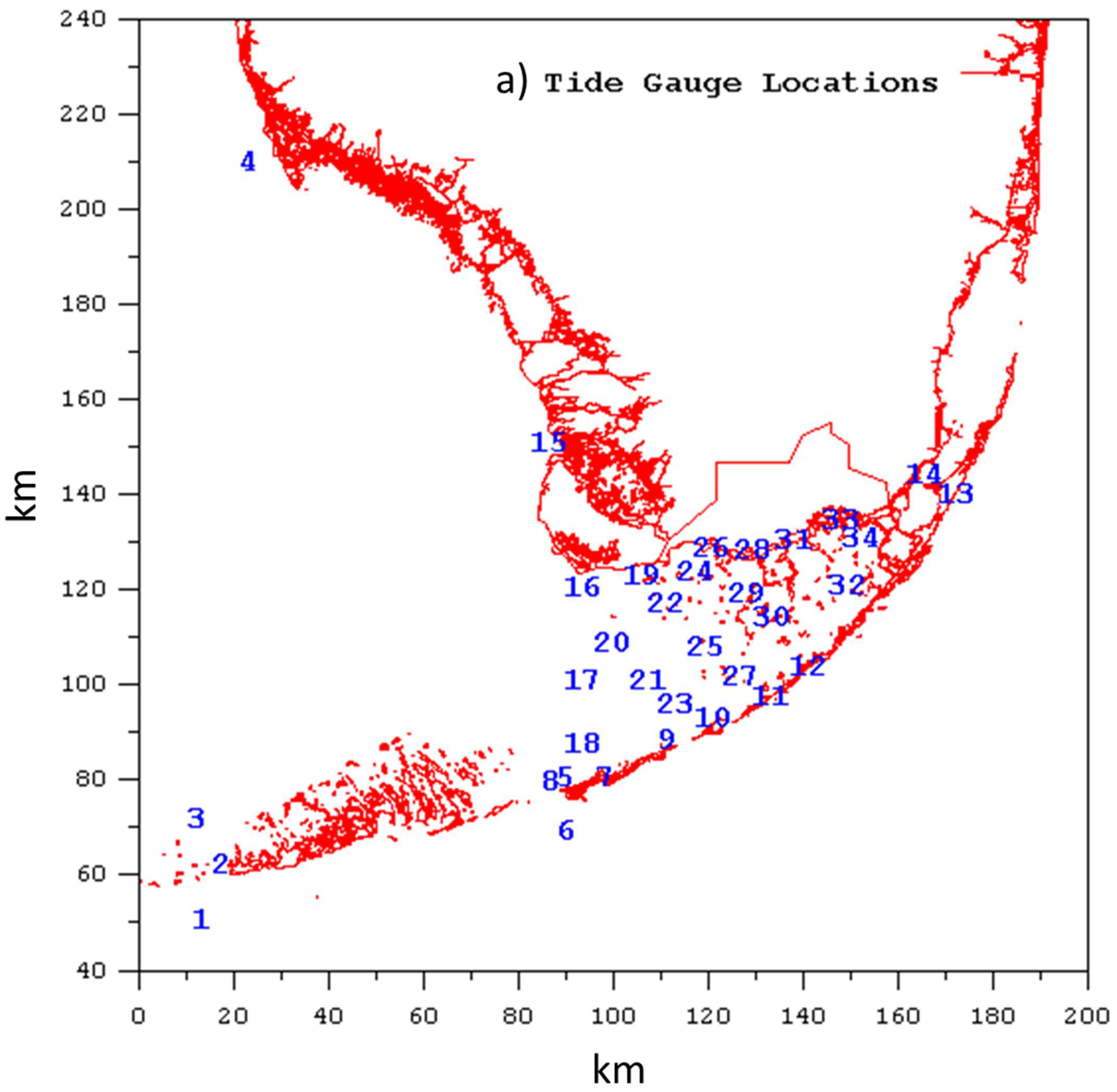
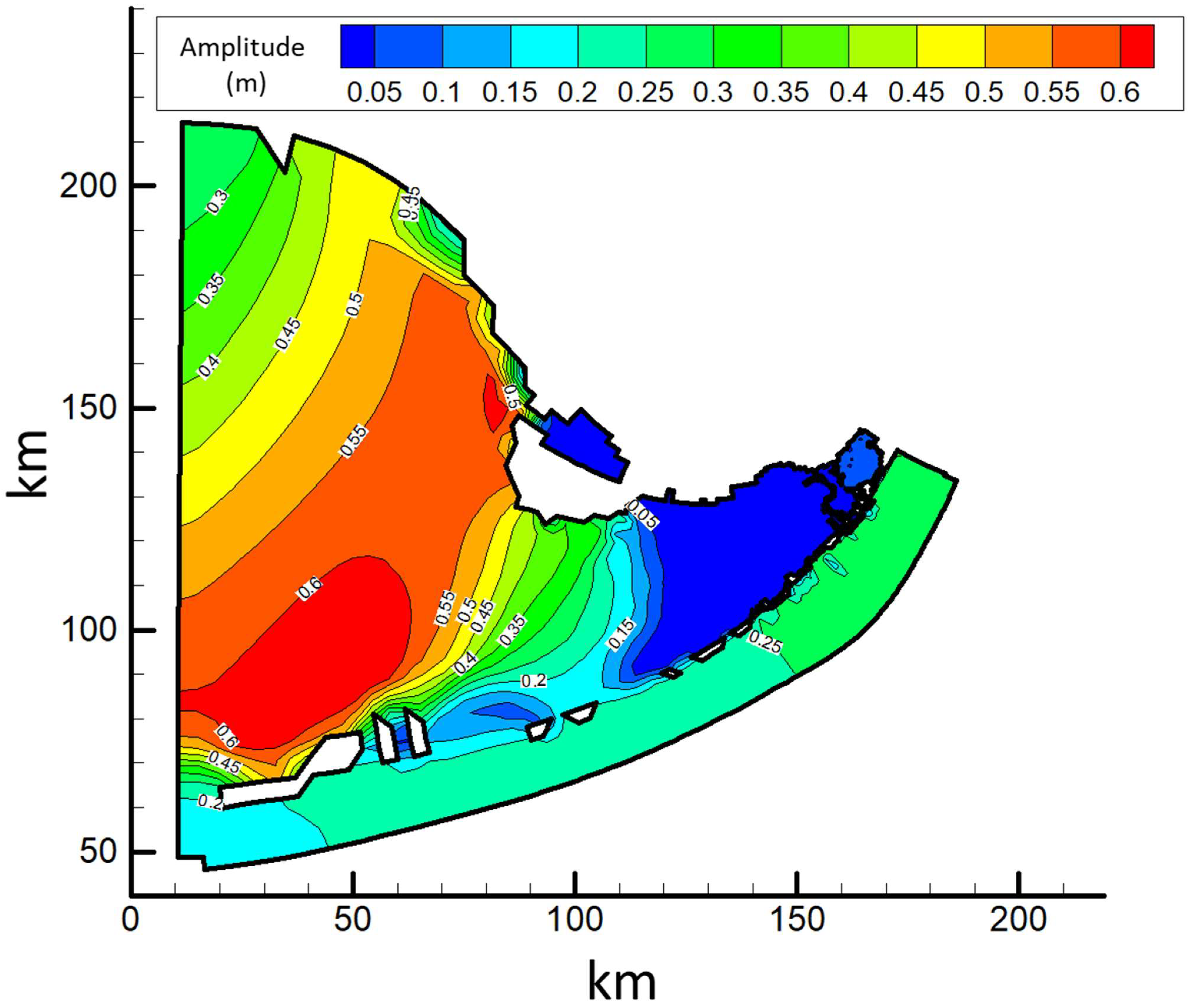
3.1. Tidal Water Surface Elevation

Table 1. Comparison of M₂ tidal water surface elevation amplitude and phase at 34 stations (refer to Figure 4a for corresponding locations denoted by ID in Column 2).

Station	ID	Observed Amplitude (cm)	Modeled Amplitude (cm)	Normalized Amplitude Error (%)	Observed Phase (min)	Modeled Phase (min)	Phase Error (min)
Sand Key	1	17.6	18.4	5	306.5	302.2	4.4
Key West	2	18.1	19.6	8	340.3	341.4	−1.1
Nav Aide	3	36.8	41.4	13	469.7	449.4	20.3
Naples	4	27.4	28.1	3	498.5	500.3	−1.7
Vaca Key	5	4.9	6.6	35	551.9	538.3	13.7
SMK	6	22.8	22.6	1	292.2	290.8	1.4
Key Colony	7	24.4	23.1	5	290.5	292.4	−1.9
TG05	8	4.8	11.3	135	356.1	342.0	14.1
TG04	9	6.6	5.0	24	287.0	299.3	−12.3
TG03	10	6.5	1.5	77	326.2	363.8	−37.6
TG02	11	20.2	25.3	25	320.7	299.0	21.6
TG01	12	13.8	26.0	88	304.5	300.0	4.4
Ocean Reef	13	27.2	30.9	14	305.1	290.4	14.7
Barnes Sound	14	8.8	8.7	1	533.6	534.6	−1.0
Shark River	15	43.1	58.8	36	581.5	593.9	−12.4
8105N	16	39.5	38.0	4	596.1	609.3	−13.2
8105C	17	36.3	29.0	20	604.3	617.6	−13.3
8105S	18	23.4	18.3	22	628.9	623.4	5.5
Murray	19	32.6	29.4	10	692.4	673.3	19.1
Oxfoot	20	37.3	28.2	24	674.8	629.7	45.1
Sprigger	21	23.4	19.3	18	652.0	651.2	0.8
Johnson	22	20.0	16.4	18	726.0	710.9	15.1
Arsenic	23	6.6	7.0	6	647.8	646.0	1.8
Buoy	24	2.7	4.1	52	145.6	93.3	52.3
Little Rabbit	25	2.7	5.0	85	188.9	703.1	−514.2
Garfield	26	1.7	2.3	35	264.6	150.7	113.9
Little Peterson	27	7.3	0.9	88	406.4	96.3	310.1
Terrapin Bay	28	0.4	1.6	300	643.8	157.8	486.0
Whipray	29	0.8	2.0	150	231.5	106.5	125.0
Bob Allen	30	4.6	0.7	85	427.1	143.3	283.8
Lt Mader	31	0.4	0.4	0	619.2	298.4	320.8
Butternut	32	0.5	0.4	20	592.9	285.2	307.7
Trout Cove	33	0.2	0.2	0	636.0	327.1	309.0
Duck	34	0.4	0.4	0	617.4	313.6	303.8

summarizes the comparison of M₂ tidal water surface elevation amplitudes and phases at 34 locations (shown in Figure 4a). There were no significant differences between tidal amplitudes and phases for the nominal coastline grid and the northeast wetland grid. The nominal coastline results are presented in Table 1. Along the western boundary at Sand Key, Key West, Nav Aide and Naples, agreement with amplitudes is within 1 cm and with phases within 5 min except for Nav Aid. Amplitude errors normalized by observed amplitudes are less than 13%. Particularly noteworthy is the behavior of tides near Key West, where amplitudes approximately double between Sand Key (Station 1 in Figure 4a) and Nav Aid (Station 3 in Figure 4a), with a phase shift of approximately three hours. The region represents a rapid transition between Florida Straits tides characterized by Sand Key and western open-boundary tides characterized by Nav Aid and Naples. The model successfully simulated the tidal behaviors in this area, despite significant changes in tides.

Deepwater stations along the southern Keys represented by SMK and Key Colony agree within 2 cm for amplitude and 2 min for phase with normalized amplitude errors being less than 5%. Tides at Vaca Key, located on the bay side of the Keys, are significantly attenuated, and the model accurately captured this phenomenon in both amplitude and phase. Model agreement with observations at the TG stations along the Keys is mixed due to the complex shoreline and bathymetry in this area. Observations at Ocean Reef and Barnes Sound agree well with model simulations because the western open boundary conditions were adjusted to optimize this agreement.

The model overpredicts tidal amplitude at Shark River, but this gauge is inland from the coastline where the model value was determined. The 8105 stations show good agreement for phase. Amplitude agreement is good at the northern station (Station 8105N), with a tendency for under-prediction moving southward. The tidal dynamics along the southern portion of the 8105 transect is strongly influenced by the interaction between tides propagating inward from the western and southern boundaries.

The intermediate interior stations, Murray through Johnson, represent the region where tides encounter the western banks of Florida Bay and become attenuated in amplitude. Further eastward, stations like Arsenic through Little Peterson and Bob Allen show continued attenuation. Tides at the interior stations (Terrapin Bay through Duck) are less than 1 cm in amplitude and have larger phase errors. Additional calibration with respect to bathymetry may improve these phases. However, given the small tidal amplitudes relative to low frequency sea level variability, which subsequently will be discussed, further calibration is likely not warranted.

Figure 5 presents a contour plot of M₂ tidal water surface elevation amplitudes, highlighting the transition from macro- to micro-tidal conditions moving eastward, attributed to mud banks attenuating tides. Analysis of other tidal constituents was also conducted, showing their amplitudes are much smaller than the M₂ tide. For instance, the second most significant constituent, S₂, typically has amplitudes less than one quarter of the M₂.

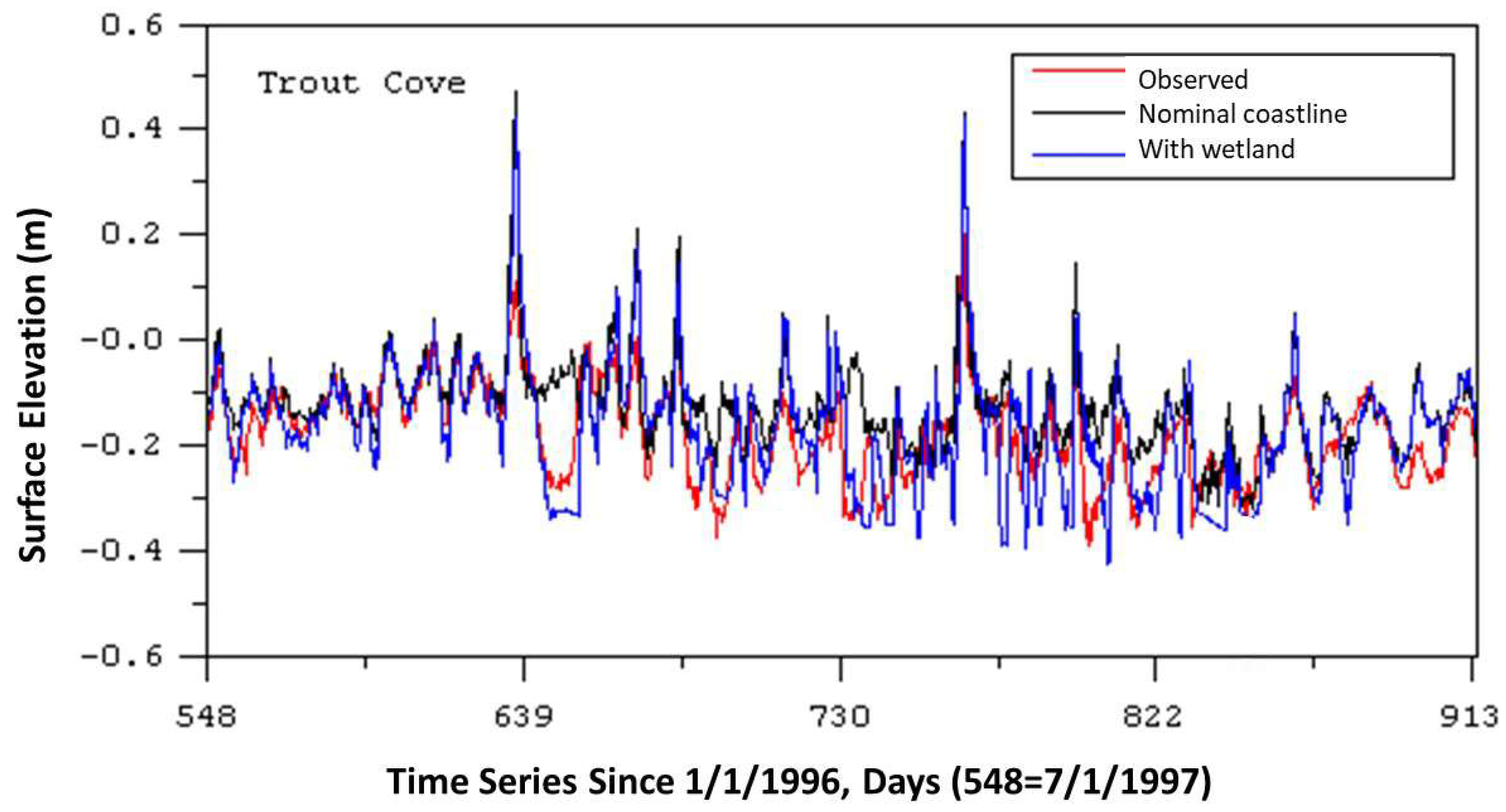
3.2. Low-Frequency Water Surface Elevation

Low-frequency water surface elevation is obtained by removing the tides. The variability of low-frequency sea level is the crucial factor influencing water surface elevation within the interior of Florida Bay. As an example, Figure 6 presents a comparison between observed and modeled low frequency sea levels at Trout Cove over 365 days, from Day 548 (1 July 1997) to Day 913 (1 July 1998). Trout Cove corresponds to Location 33 in Figure 4a. The figure reveals that both grid configurations, the nominal coastline version and the northeast wetland version, effectively capture observed sea level variations. Notably, the grid with the wetland performs better in representing rapid sea level drops after high-sea-level events at Trout Cove (for example, just after Day 639 and Day 730). This can be attributed to the fact that the inclusion of the wetland along the northern boundary allows a north–south seiche response.

Table 2. Comparison of low-frequency water surface elevations (see Figure 4a for Trout Cove Location 33 and Terrapin Bay Location 28).

Station/Configuration	Absolute Relative Error (%)	RMS Error (cm)
Trout Cove Nominal Coastline	5.9	8.1
Trout Cove Northeast Wetland	6.6	8.7
Terrapin Bay Nominal Coastline	8.8	12.7
Terrapin Bay Northeast Wetland	8.6	12.5

provides a summary of the time series error analysis for two stations: Trout Cove and Terrapin Bay (Station 28 in Figure 4a). Root mean square errors (RMS) at Trout Cove are less than 9 cm, and when normalized by an absolute range of 60 cm, absolute relative errors are less than 9%.

An important conclusion from the measured data is that the low frequency sea level variability in the interior of Florida Bay is approximately 60 cm, compared to astronomical tide ranges typically less than 2–4 cm (as shown in Table 1). Thus, in addition to buoyant inflow, low frequency subtidal sea level variability is a primary factor controlling dynamics in the eastern interior of Florida Bay.

As depicted in Figure 5, tides play a significant role in the western open water areas and along the northwest coast, while they are relatively small in the central and northeast regions of Florida Bay due to shallow bathymetry attenuating tidal influence. Wind-driven flows and long-term fluctuations in sea level from the open boundary in the Gulf of Mexico dominate mixing and exchange processes. Given that the subtidal sea level variation can exceed 60 cm, it plays a pivotal role in driving water exchange with the adjacent coastal waters of the Atlantic Ocean and the Gulf of Mexico. During periods of low sea level, connections between adjacent basins (as shown in Figure 1) are restricted, minimizing overbank exchange. Conversely, high water levels facilitate more freshwater from the Everglades across the shallow banks into the central and southern regions of the bay.

3.3. Tidal Currents

Table 3 summarizes the comparison of M₂ horizontal tidal current major axis amplitudes, phases, and orientation angles at 42 locations (shown in Figure 4b). Here are key observations:

(1)

Station IDs 1 through 9 correspond to locations in the Florida Straits (to the south of the Keys). Observed tidal current amplitudes in this area are less than 5 cm/s. The model simulation is judged as good for amplitudes and fair for phases and orientations.

(2)

Stations with IDs 11 through 19 represent major openings between the western region of the bay and the straits. Current amplitudes at these stations are relatively large, between 25 and 90 cm/s. Model simulations of amplitudes, phases, and orientations are quite good, with phases within approximately 20 min or less and angles within 26 degrees or less. Considering that the modeled velocities are averages over 10⁵ to 10⁶ km² and are compared to a single-point current measurements, the agreement of amplitudes is adequate.

(3)

Stations with IDs 20 through 24 represent the southwest region of the bay. Agreement between amplitudes at these stations is again adequate. With the exception of Station 24, phase differences are less than 20 min, and angle differences are less than 7 degrees.

(4)

Stations with IDs 25 through 32 represent the western central region of the bay. Agreement at Stations 25 and 26 is good. Agreement at Stations 27 through 32 is much more variable due to the influence of banks and local features controlling current dynamics.

(5)

Stations 33, 34, 37, and 38 are representative of the southwest coastal shelf outside of Florida Bay. At the two southern stations, 33 and 34, the current amplitudes are simulated well, and the phases and angles are within approximately 12 min and 22 degrees. At the northern station 37, which is on the model’s open boundary, the simulated currents agree well with the observed data, while the phase error is on the order of 1 h. Angular error at this station is a low 6 degrees. Amplitude and angle agreement at Station 38 is exceptionally good and the phase error is less than 25 min.

(6)

At Stations 35 and 36, the model tends to underpredict current amplitudes in this region but does exceptionally well with respect to phase and angle.

(7)

Stations with IDs 39 through 42 represent the Whipray Basin region of the central Florida Bay. Although the model calculates the appropriate magnitudes of the relatively low current amplitudes, agreements in phase and direction are quite variable and likely associated with bathymetric features that are not well resolved in the grid.

Overall, the model reasonably captures the horizontal M₂ tidal currents, considering its flux-based dynamics. Refinement could be achieved with more accurate bottom bathymetry data.

Table 3. Horizontal current M₂ major axis amplitude, phase and orientation comparison at 42 stations (see Figure 4b for locations corresponding to ID in Column 2).

Station	ID	Observed Major Axis (cm/s)	Modeled Major Axis (cm/s)	Observed Phase at Major (min)	Modeled Phase at Major (min)	Observed Major Direction (Degree)	Modeled Major Direction (Degree)
Tennessee	1	4.3	6.1	316.8	235.2	17	71
Allig Reef	2	3.3	3.5	21.0	121.2	42	64
Hawk IM	3	3.3	3.5	304.5	471.0	36	99
Triangles	4	3.3	4.7	366.2	485.5	79	116
Conch Reef	5	4.9	5.9	15.7	121.3	58	103
Molasses	6	5.0	5.4	14.0	104.2	54	104
Hawk MK	7	3.6	3.4	197.8	130.2	38	−50
Pacific Rf	8	3.1	4.4	411.8	247.7	81	67
MKR 4 Hk	9	2.0	6.2	96.8	222.5	62	63
NW Chan	10	65.9	59.7	200.3	165.0	120	84
7 MiBr 7	11	27.4	45.0	274.3	264.7	122	112
7 MiBr 5	12	35.1	55.7	284.3	272.0	98	100
7 MiBr 3	13	43.7	50.4	287.2	281.2	118	95
7 MiBr 2	14	63.6	57.3	291.5	287.8	103	79
Moser	15	52.8	50.4	296.7	281.2	94	95
Knight Ky	16	89.4	57.3	292.7	287.8	54	79
Long Ky	17	54.8	59.1	299.3	312.8	137	163
Indian Key	18	47.4	24.3	242.0	294.8	135	125
Tea Table	19	45.8	24.3	248.0	294.8	94	124
8105 S	20	15.3	17.3	278.5	282.7	82	84
S South	21	8.4	16.6	320.0	322.2	48	47
Chan Key	22	42.3	32.2	320.8	304.3	171	175
Long Ky	23	45.9	27.5	304.9	314.8	112	119
Yacht Ch	24	44.1	23.5	226.7	310.7	37	−39
8015 C	25	27.4	24.1	179.0	195.3	144	146
S-Central	26	20.0	23.1	204.9	211.0	130	138
Rabbit Ky	27	41.4	22.9	373.8	317.7	7	3
S Twin Ky	28	56.9	16.2	406.4	353.2	148	140
Gopher Ky	29	45.9	14.9	408.2	359.5	166	154
Spy Key	30	3.3	9.4	451.0	329.3	4	25
N Central	31	19.6	27.3	154.4	168.5	161	158
N Central	32	4.5	8.2	451.6	325.3	−40	7
NOAA B	33	27.0	33.4	386.7	377.5	−19	3
NOAA A	34	28.2	31.9	427.0	415.5	2	4
8105 N	35	38.9	26.7	147.2	144.3	167	174
Flamingo	36	36.4	19.8	216.5	216.5	5	0
NOAA D	37	24.6	32.9	396.2	323.7	166	160
NOAA C	38	24.6	25.9	407.2	383.7	2	12
Crock D	39	0.3	2.0	210.5	82.3	114	159
Dump W	40	1.6	3.5	307.0	92.7	81	68
Topsy D	41	0.2	4.0	428.5	269.0	125	68
Twisty W	42	0.3	2.7	57.8	165.7	169	109

Table 3. Horizontal current M₂ major axis amplitude, phase and orientation comparison at 42 stations (see Figure 4b for locations corresponding to ID in Column 2).

Station	ID	Observed Major Axis (cm/s)	Modeled Major Axis (cm/s)	Observed Phase at Major (min)	Modeled Phase at Major (min)	Observed Major Direction (Degree)	Modeled Major Direction (Degree)
Tennessee	1	4.3	6.1	316.8	235.2	17	71
Allig Reef	2	3.3	3.5	21.0	121.2	42	64
Hawk IM	3	3.3	3.5	304.5	471.0	36	99
Triangles	4	3.3	4.7	366.2	485.5	79	116
Conch Reef	5	4.9	5.9	15.7	121.3	58	103
Molasses	6	5.0	5.4	14.0	104.2	54	104
Hawk MK	7	3.6	3.4	197.8	130.2	38	−50
Pacific Rf	8	3.1	4.4	411.8	247.7	81	67
MKR 4 Hk	9	2.0	6.2	96.8	222.5	62	63
NW Chan	10	65.9	59.7	200.3	165.0	120	84
7 MiBr 7	11	27.4	45.0	274.3	264.7	122	112
7 MiBr 5	12	35.1	55.7	284.3	272.0	98	100
7 MiBr 3	13	43.7	50.4	287.2	281.2	118	95
7 MiBr 2	14	63.6	57.3	291.5	287.8	103	79
Moser	15	52.8	50.4	296.7	281.2	94	95
Knight Ky	16	89.4	57.3	292.7	287.8	54	79
Long Ky	17	54.8	59.1	299.3	312.8	137	163
Indian Key	18	47.4	24.3	242.0	294.8	135	125
Tea Table	19	45.8	24.3	248.0	294.8	94	124
8105 S	20	15.3	17.3	278.5	282.7	82	84
S South	21	8.4	16.6	320.0	322.2	48	47
Chan Key	22	42.3	32.2	320.8	304.3	171	175
Long Ky	23	45.9	27.5	304.9	314.8	112	119
Yacht Ch	24	44.1	23.5	226.7	310.7	37	−39
8015 C	25	27.4	24.1	179.0	195.3	144	146
S-Central	26	20.0	23.1	204.9	211.0	130	138
Rabbit Ky	27	41.4	22.9	373.8	317.7	7	3
S Twin Ky	28	56.9	16.2	406.4	353.2	148	140
Gopher Ky	29	45.9	14.9	408.2	359.5	166	154
Spy Key	30	3.3	9.4	451.0	329.3	4	25
N Central	31	19.6	27.3	154.4	168.5	161	158
N Central	32	4.5	8.2	451.6	325.3	−40	7
NOAA B	33	27.0	33.4	386.7	377.5	−19	3
NOAA A	34	28.2	31.9	427.0	415.5	2	4
8105 N	35	38.9	26.7	147.2	144.3	167	174
Flamingo	36	36.4	19.8	216.5	216.5	5	0
NOAA D	37	24.6	32.9	396.2	323.7	166	160
NOAA C	38	24.6	25.9	407.2	383.7	2	12
Crock D	39	0.3	2.0	210.5	82.3	114	159
Dump W	40	1.6	3.5	307.0	92.7	81	68
Topsy D	41	0.2	4.0	428.5	269.0	125	68
Twisty W	42	0.3	2.7	57.8	165.7	169	109

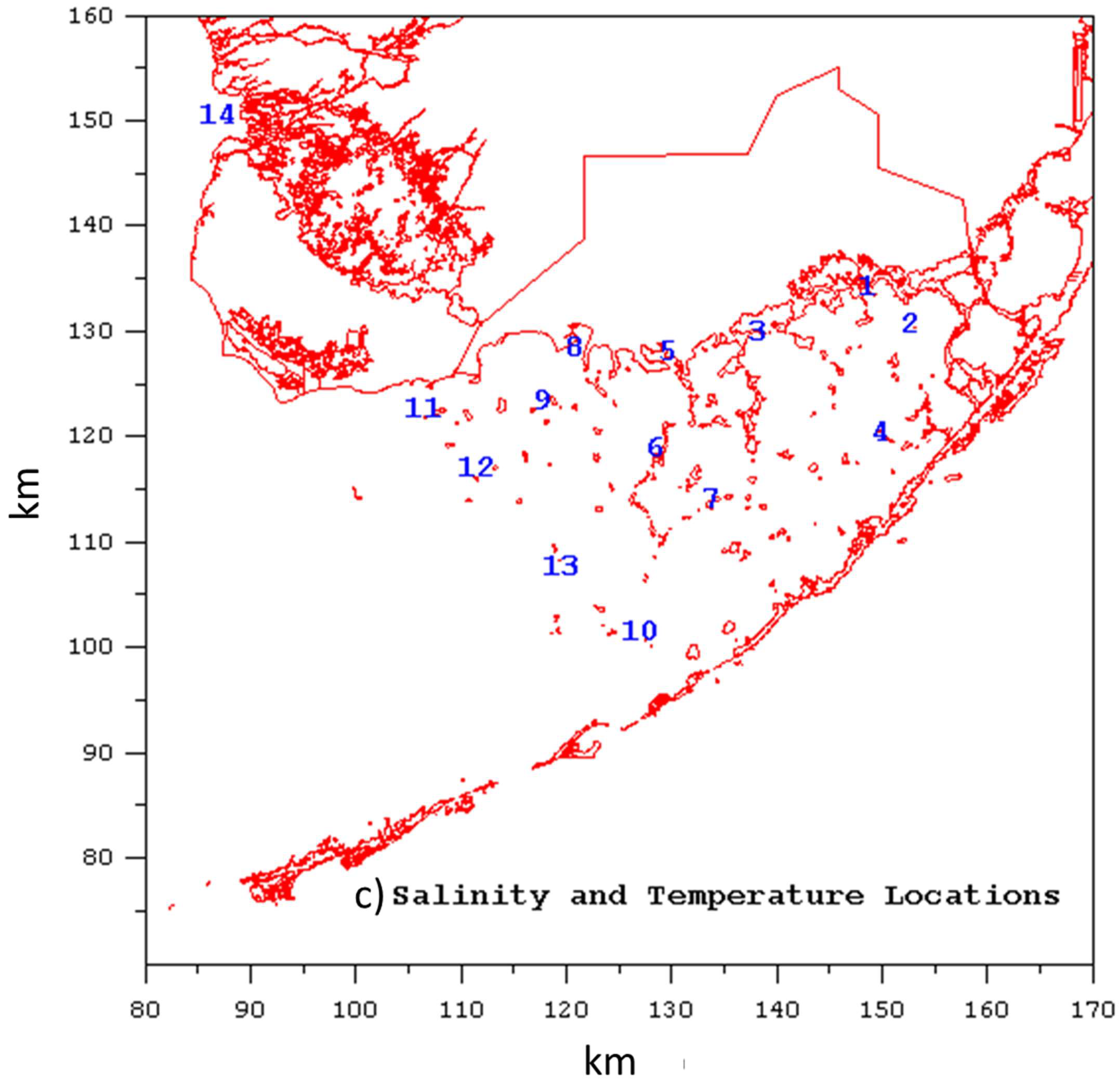
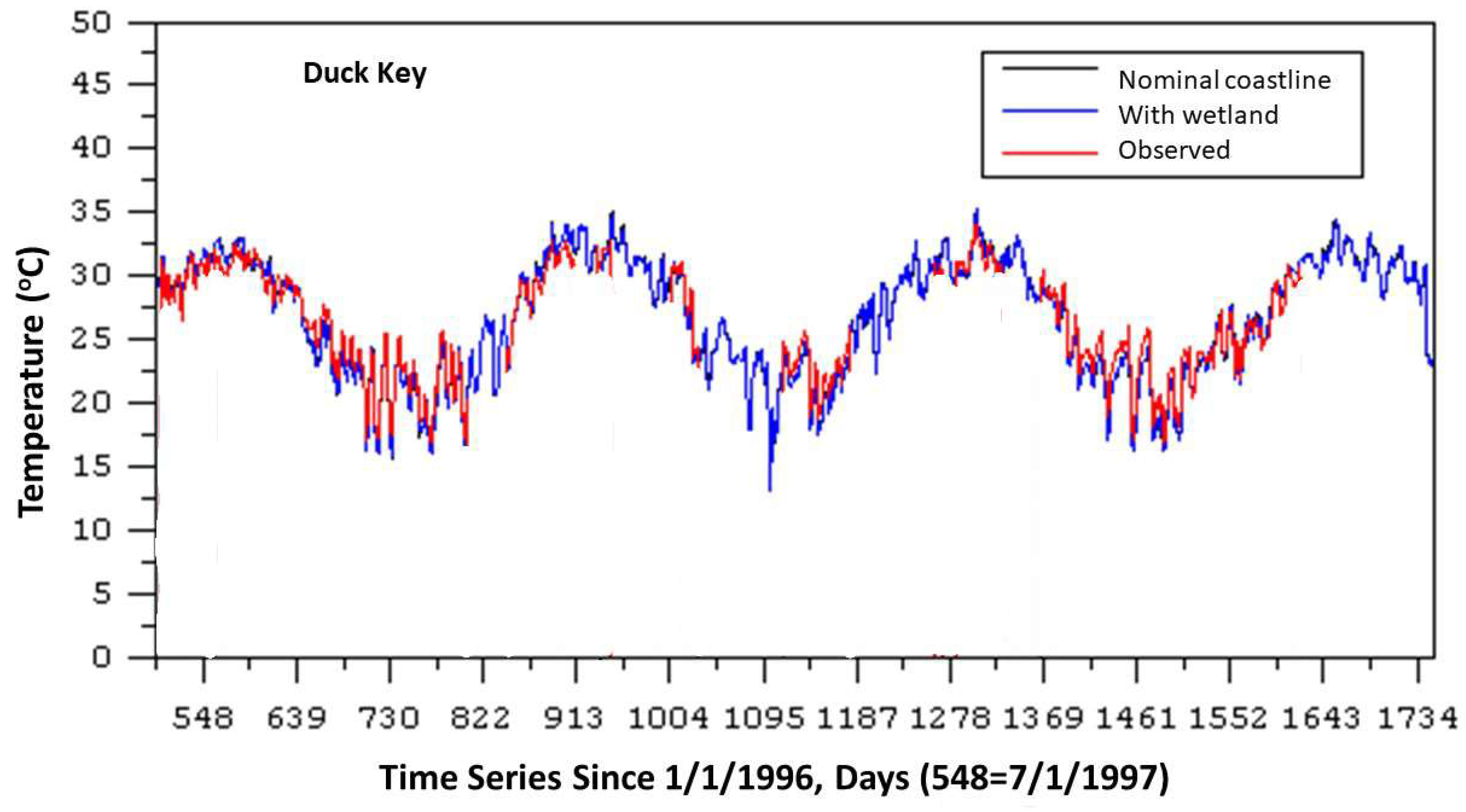
3.4. Temperature Calibration

Temperature calibration involved solely adjusting incoming solar radiation. Since direct observations of solar radiation were unavailable for the entire simulation period, model input values were initially estimated using cloud cover to adjust theoretical values, dependent on time and location. The estimated values were later refined through a comparison with observed radiation data spanning approximately 3 years of the 7-year simulation period.

The quantitative evaluation of the temperature calibration utilized continuous observational data at 14 ENP stations.

Table 4. Error analysis of temperature simulation at 14 ENP stations (see Figure 4c for locations corresponding to ID in Column 2).

Station	ID	RMS Error With Nominal Coastline (°C)	RMS Error with Wetland (°C)	Normalized RMS Error with Nominal Coastline (%)	Normalized RMS Error with Wetland (%)
Trout Cove	1	1.49	1.29	6	5
Duck Key	2	0.96	0.96	4	4
Little Maderia Bay	3	1.21	1.28	5	5
Butternut Key	4	1.92	1.91	7	7
Terrapin Bay	5	1.40	1.43	5	5
Whipray	6	1.47	1.47	5	5
Bob Allen	7	1.45	1.45	5	5
Garfield	8	2.92	2.89	11	11
Buoy Key	9	1.27	1.27	5	5
Peterson	10	1.32	1.33	5	5
Murray	11	3.48	3.47	13	13
Johnson	12	1.25	1.25	5	5
Little Rabbit	13	1.20	1.20	5	5
Shark River	14	1.25	1.25	5	5

summarizes the error analysis of temperature simulation at these stations for the 7-year modeling period. Normalized RMS errors at 12 of the stations are less than 7%, while at Garfield and Murray, the normalized RMS errors are less than 13%. Overall, these low normalized errors are well below the general criteria of 15% for transport simulation accuracy [31].

As an example, Figure 7 illustrates a time series plot of depth-averaged model temperature and observations taken at an i location in the water column at Duck Key. Visual agreement is quite good. Discrepancies at these stations are attributed to shallow water column depths, resulting in excessive heating. The model is modified to absorb a portion of the incoming solar radiation into the bed layer to provide a more realistic representation of radiation absorption.

3.5. Salinity Calibration

Salinity is a fundamental characteristic of estuarine and coastal ecosystems, significantly influencing water quality, the composition and spatial distribution of vegetative communities, and the life of various animal species. The dynamic simulation of the spatial distribution of salinity on annual time scales is crucial for estuarine hydrodynamic models and is a prerequisite for driving water quality models [1].

Simulating salinity in Florida Bay presents challenges due to uncertainties in several key components of the salt balance. The representation of saltwater intrusion into the interior of Florida Bay, from the southern and western ocean boundaries, is dependent upon the detailed representation of the bay’s bathymetry. Large regions of the bay are too shallow to be surveyed by conventional means and essentially require an estimation of their bottom elevations. Creeks and rivers discharging along the northern and eastern boundaries of the bay and the southwest Florida coast have been extensively gauged since 1996. However, distributed surface and groundwater exchange between the bay and the Everglades remains poorly quantified. Evaporation, the other major component of the salt balance, is difficult to calculate on daily time scales due to its high degree of spatial and temporal variability and its embedding in the thermal dynamics of the system. In addition, salinities in the bay are influenced by interannual cycles and decadal variability [28].

Salinity generally varies with the annual wet and dry seasons driven by regional precipitation and temperature patterns in subtropical south Florida. It also responds to episodic meteorological events like tropical storms and cold fronts. Error analyses of salinity simulations are presented in

Table 5. Error analysis of salinity simulation at 14 ENP stations (see Figure 4c for locations corresponding to ID in Column 2).

Station	ID	RMS Error With Nominal Coastline (ppt)	RMS Error with Wetland (ppt)	Normalized RMS Error with Nominal Coastline (%)	Normalized RMS Error with Wetland (%)
Trout Cove	1	14.18	8.08	75	43
Duck Key	2	3.28	4.11	13	16
Little Maderia Bay	3	4.31	7.20	21	34
Butternut Key	4	3.93	5.27	14	18
Terrapin Bay	5	6.46	7.15	26	28
Whipray	6	4.04	5.64	12	17
Bob Allen	7	3.53	4.39	11	13
Garfield	8	6.32	15.11	21	50
Buoy Key	9	5.70	9.13	17	28
Peterson	10	2.89	2.94	8	9
Murray	11	4.39	5.61	14	17
Johnson	12	4.69	5.97	14	18
Little Rabbit	13	4.03	4.77	12	14
Shark River	14	5.88	6.10	24	25

. The Trout Cove station exhibits high salinity due to the largest freshwater inflow. The Duck Key station performs well for both configurations, with only 13% and 16% normalized RMS errors. Little Maderia Bay is also highly influenced by freshwater inflows, with the nominal coastline configuration producing a lower normalized RMS error of 21%. Butternut Key displays good performance, with normalized RMS errors of 14% and 18%. Terrapin Bay is strongly influenced by inflows. Although the normalized errors slightly exceed 25%, a visual comparison shows a strong agreement with observed salinity variation. Modeled salinity is very good at Whipray in the central region of Florida Bay, with low normalized RMS errors of 12% and 17%. At Bob Allen, the model generally corresponds well. Agreement at Garfield is highly variable in response to freshwater inflows in the area. Agreements at Buoy Key, Murray, Johnson, and Little Rabbit are quite similar, exhibiting similar time periods of under- and over-prediction. Normalized error measures are all between 12% and 18%, except for the higher value at Buoy for the wetland grid configuration. Peterson (Station 10 in Figure 4c) is the least influenced by freshwater inflow of the 14 stations, showing salinity variation in response to only the highest inflow events. Shark River represents the lower southwest coast and has normalized RMS errors of 24% and 25%.

As an example, Figure 8 shows a comparison of observations and modeled salinity at Duck Key using the nominal coastline and the northeast wetland configurations. Lower-salinity conditions are associated with episodic events such as tropical storms or above-average rainfall. Through visual and quantitative assessment (refer to Table 5), both the nominal coastline and the wetland configurations perform well in calculating salinity. Overall, the nominal coastline configuration, which introduces net freshwater inflows at points along the nominal coastline, yields superior error measures. A refinement of the wetland’s configuration incorporating groundwater interaction could likely enhance the accuracy of the wetland configuration.

Figure 9 presents the modeled salinity on Day 1404 (5 November 1999). The insert in Figure 9 shows the patterns of total freshwater inflow during the seven years of the simulation period (1996–2002). The green line indicates that Day 1404 has a relatively high inflow. Salinity variability in Figure 9 is most pronounced in the northeast, diminishing toward the west. This pattern reflects the dynamic interplay of the freshwater inflow, the continuous exchange of water with the coastal ocean and the Gulf of Mexico, variation in evaporation, and physical circulation effects. Freshwater inflow from the Everglades dilutes the salinity in the northeast of the bay, while exchange with the Florida Straits and the Gulf of Mexico replaces diluted estuarine water with water of higher salinity and greater density. Thus, the changes in salinity, both temporally and spatially, are driven by three key processes: the net supply of freshwater, the mechanisms governing mixing within the estuary (such as wind, topography, and currents), and the exchange of salinity with the coastal ocean.

4. Impacts of Open Boundary Forcings and Grid Resolution

Estuarine and coastal modeling often faces the challenge of how to specify appropriate open boundary conditions (OBCs) and select optimum grid resolution, which are also two essential issues in setting up the FBM.

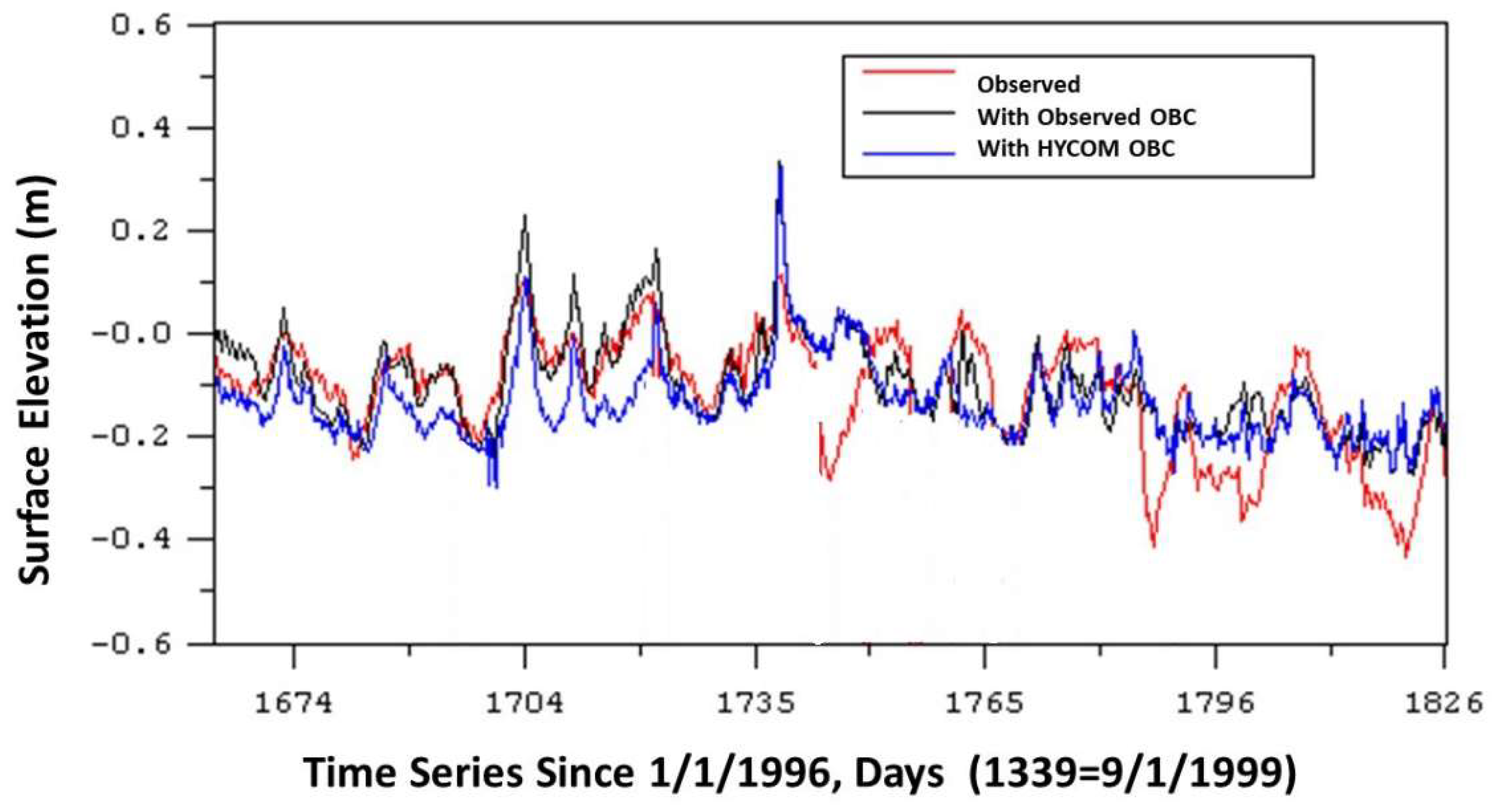
4.1. Interfacing with Another Ocean Model

The OBCs of an estuarine model need data from either observations or another model with a larger domain that covers the study area. There have been many studies on the subject of OBC. For example, Marsaleix et al. [32] reviewed the usual open boundary conditions (OBCs) for coastal ocean models and proposed a complete set of open boundaries based on stability criteria, mass and energy conservation arguments, and the ability to enforce external information. Diederen et al. [33] introduced a new equation describing hydrodynamics in infinitely long tidal channels under the influence of oceanic forcing. In a modeling study, Liu and Gan [34] examined estuarine–shelf circulation using a composite tidal and subtidal open boundary condition, accommodating the circulation driven by regional tides, subtidal forces, and external forcing.

The FBM described in Section 2 utilized measured data to specify the OBC, which is a preferred approach. In the absence of measured data, another common approach is to employ results from another ocean model with a larger domain. The HYbrid Coordinate Ocean Model (HYCOM) has been applied to the Gulf of Mexico for many years (e.g., [35,36]). To understand the ability of the FBM to accept low-frequency hydrodynamic OBCs from HYCOM, a 16-month simulation, from September 1999 to December 2000, was conducted with the nominal coastline version of the grid. All forcing functions remained the same, except that the low-frequency components of OBCs were replaced by results from the HYCOM simulation, including water surface elevation and barotropic current.

Figure 10 represents a comparison of low-frequency water surface elevations at Key West (the western boundary of the FBM) between HYCOM simulated results and the observed data. The figure indicates that HYCOM simulated some general features of the observations but exhibited less variability and extended periods of underestimation and overestimation. A notable concern is the mismatch in the first 90 days and the absence of the observed extreme high sea level around Day 1380 that coincided with the time of the largest freshwater inflow to the bay.

Figure 11 depicts low-frequency water surface elevations at Trout Cove from the observed data, the simulation with observation-based OBCs and the simulation with HYCOM-based OBCs. Despite large differences in OBC (shown in Figure 10), the results using HYCOM OBCs are reasonably good and are much better than might be anticipated from the comparison in Figure 10 regarding the western OBC. This supports the conclusion that wind forcing is primarily responsible for observed subtidal sea level variability in the bay’s interior. While the observed sea level at Key West (Figure 10) responds to regional wind forcing and nonlocal mechanisms, the observation-based OBC remains superior, yielding an RMS error of 8.6 cm, compared to the 10.6 cm RMS error for HYCOM-based OBC.

Modeled salinities from the observation-based OBC and the HYCOM-based OBC are also compared. The two OBC cases exhibit insignificant differences in salinity simulation. This reaffirms that local wind forcing is primarily responsible for transport associated with low-frequency sea level variability. Among the external forcings, wind and freshwater inflows are the primary factors controlling the salinity process. While HYCOM-OBCs for the FBM are deemed adequate, they should be used in conjunction with observational wind forcing fields to accurately simulate sea level variability and salinity in the interior of Florida Bay.

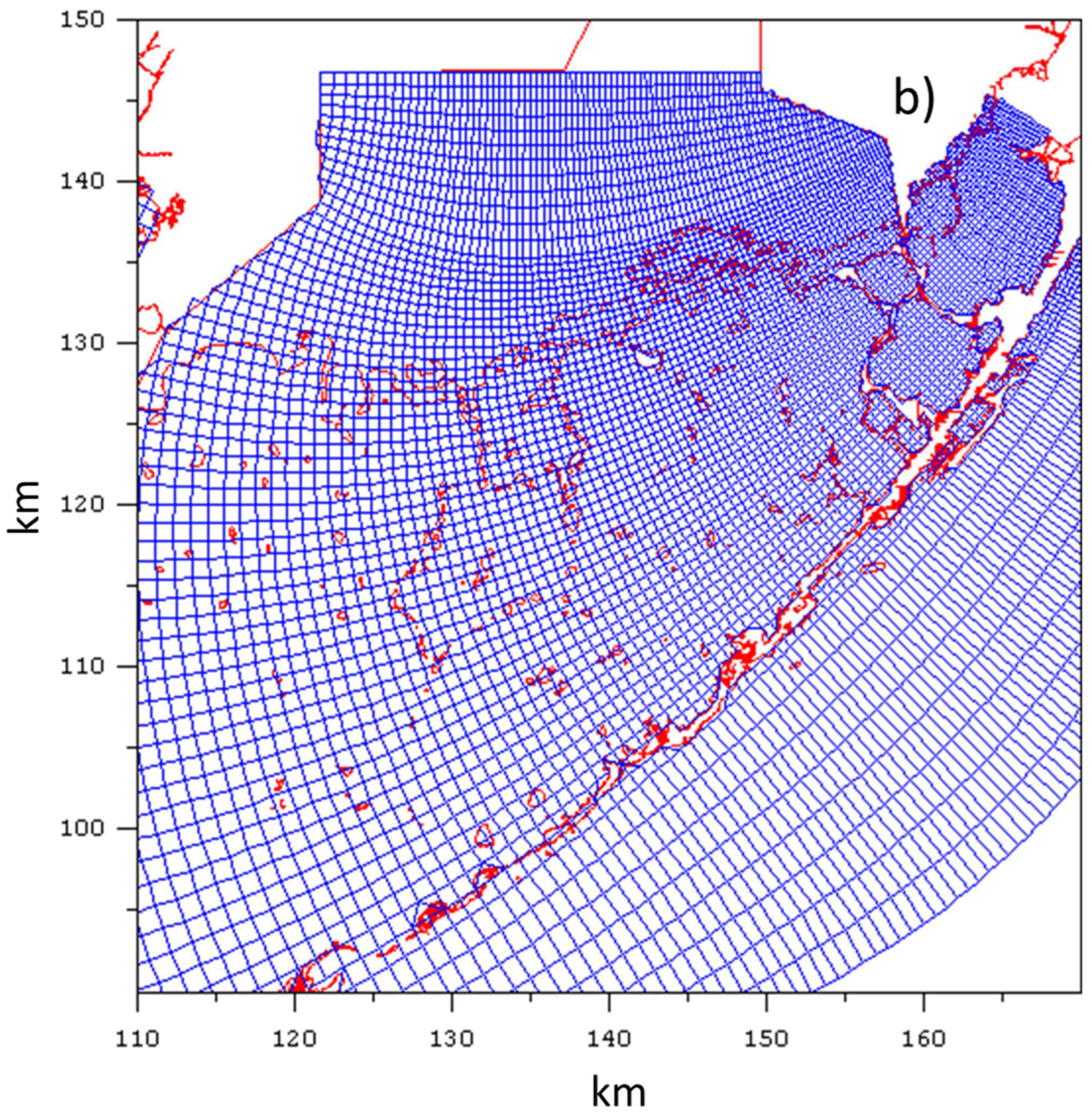
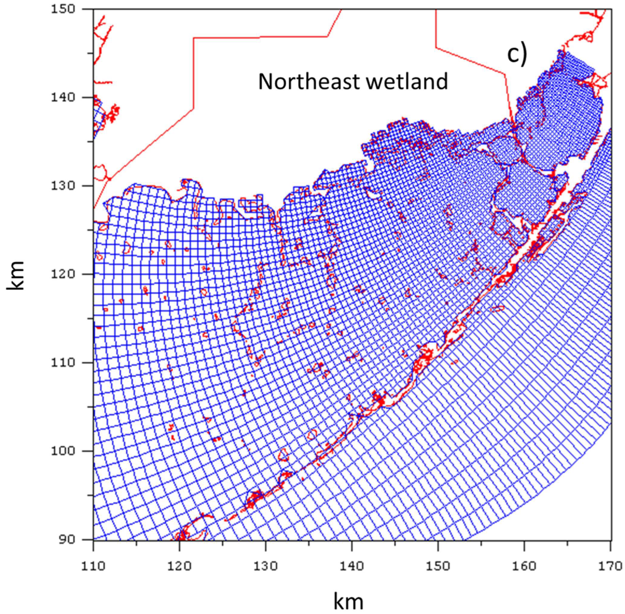
4.2. Grid Resolution Analysis

Grid resolution is a crucial aspect in the development of hydrodynamic and water quality models, with various studies emphasizing the selection of optimum resolutions in both the horizontal and the vertical directions. For instance, Andrejev et al. [37] discussed the role of spatial resolution in a three-dimensional hydrodynamic model for marine transport risk assessment. Hasan et al. [38] found that increasing grid resolution improved the agreement of computed flow velocities with field observations in the Johor Estuary, Singapore. They highlighted that enhancing the alignment of the grid with channel boundaries, with a more modest increase in resolution, significantly improved model performance. This grid modification notably impacted computed salinity in the estuary, while water levels were only slightly affected. Ralston et al. [39] assessed a 3D unstructured grid finite-volume hydrodynamic model against shipboard and moored observations, reporting that a coarse grid led to increased numerical mixing, necessitating further reductions in turbulent mixing and greater bed friction for optimization. Nwogwu et al. [40] used the EFDC model to simulate water surface elevation, comparing results with three grid resolutions—fine, medium, and original—and found similar performance for each.

The modeling system for Florida Bay should support decadal timescale simulations to evaluate alternative restoration-impact-management scenarios. A comprehensive alternative evaluation, involving model configuration, execution, and prediction analysis, should be achievable within a reasonable timeframe. An analysis of grid resolution requirements for the FBM aims to determine the sensitivity of model results to horizontal and vertical spatial resolution. The objective is to identify optimal horizontal and vertical spatial resolutions at which future grid refinement or increased spatial resolution yields marginal performance improvements relative to computational effort.

The original horizontal grid consists of approximately 4300 cells, with cell sizes ranging from about 500 m in the eastern interior of the bay to around 8 km at the western open boundary in the Gulf of Mexico. A fine grid was created by nesting four horizontal cells within each cell of the original grid, effectively doubling the horizontal spatial resolution. The fine horizontal grid comprises approximately 17,200 cells, with cell sizes ranging from approximately 250 m in the eastern interior of the bay to around 4 km at the western open boundary in the Gulf of Mexico.

The USGS Florida Bay bathymetric survey data served as the primary information source for comparison. The data set, in addition to providing bathymetry, delineates shallow mud banks, shoals, and cuts and passages through the banks. Track lines from the bathymetric survey were overlaid on the two horizontal grids and visual inspection was conducted to assess the resolution of shoreline features and shallow banks. The analysis revealed that the original grid only approximated the location and widths of the banks, while the fine grid’s spatial resolution was consistent with the banks, providing a better approximation of their locations.

The quantitative analysis involved three pairs of comparative model simulations, spanning a three-year period from mid-1997 to mid-2000. Comparative assessments included tidal harmonic amplitudes and phases of water surface elevation and horizontal currents, as well as salinity simulations.

The first pair of simulations compared the original grid with a single vertical layer (depth average) against the original grid with two vertical layers. Evaluation based on daily averaged model-predicted and observed salinity at 14 ENP locations showed a substantial reduction in RMS errors for the two-layer grid at six stations, marginal reduction at six stations, and a slight increase at two stations. The two-layer simulation demonstrated salinities in closer agreement with observations, showing significant improvements in response to tropical storms. The use of two layers resulted in an overall reduction of approximately 12% in RMS errors. RMS differences between salinities calculated using the single- and two-layer grids ranged from 0.27 and 7.57 ppt. The visual inspection of time series plots indicated a substantial improvement in model prediction with the two-layer grid.

A second pair of simulations compared two- and four-layer versions of the original horizontal grid, with the overall performance of the four-layer simulation showing no substantial difference from the two-layer one. This suggested that using two vertical layers was appropriate for evaluating horizontal grid resolution.

The third pair of simulations compared the original and fine grids, both with two layers in the vertical. RMS error comparisons indicated that the fine grid yielded no significant or consistent change. The fine grid showed a maximum reduction of approximately 20% in RMS error over the original grid at one station, while the maximum increase in RMS error was approximately 25% at another station. Normalized RMS differences between the original and fine-grid salinity simulations were less than 10% at 12 of the 14 locations of time series comparison. Visual comparison of time series plots revealed little difference between the original and fine grid predictions. Also, in light of the approximately eight-fold increase in computational requirements for the fine horizontal grid over the original horizontal grid, any increases in modeling performance with respect to observations should be evaluated in an incremental trade-off manner.

The major conclusions from the grid resolution analysis are as follows: (1) the most significant improvement in model performance is achieved by increasing the vertical resolution to two layers; (2) the four-layer simulation performance does not substantially differ from the two-layer one; and (3) a fine horizontal grid, with a two-fold increase in horizontal resolution or four times as many horizontal cells, does not achieve a well-defined increase in model performance relative to an approximately eight-fold increase in computational effort.

5. Summary and Conclusions

This study focuses on the hydrodynamic modeling of Florida Bay, a large, shallow estuary in subtropical Florida. Here are the major results and conclusions.

• Based on the EFDC model, the three-dimensional hydrodynamic model of Florida Bay was calibrated using a comprehensive dataset, including measurements over 7 years at 34 tidal stations, 42 current stations, and 14 temperature and salinity stations. Overall, the FBM simulated tides, low-frequency surface water elevation, current, temperature, and salinity reasonably well.
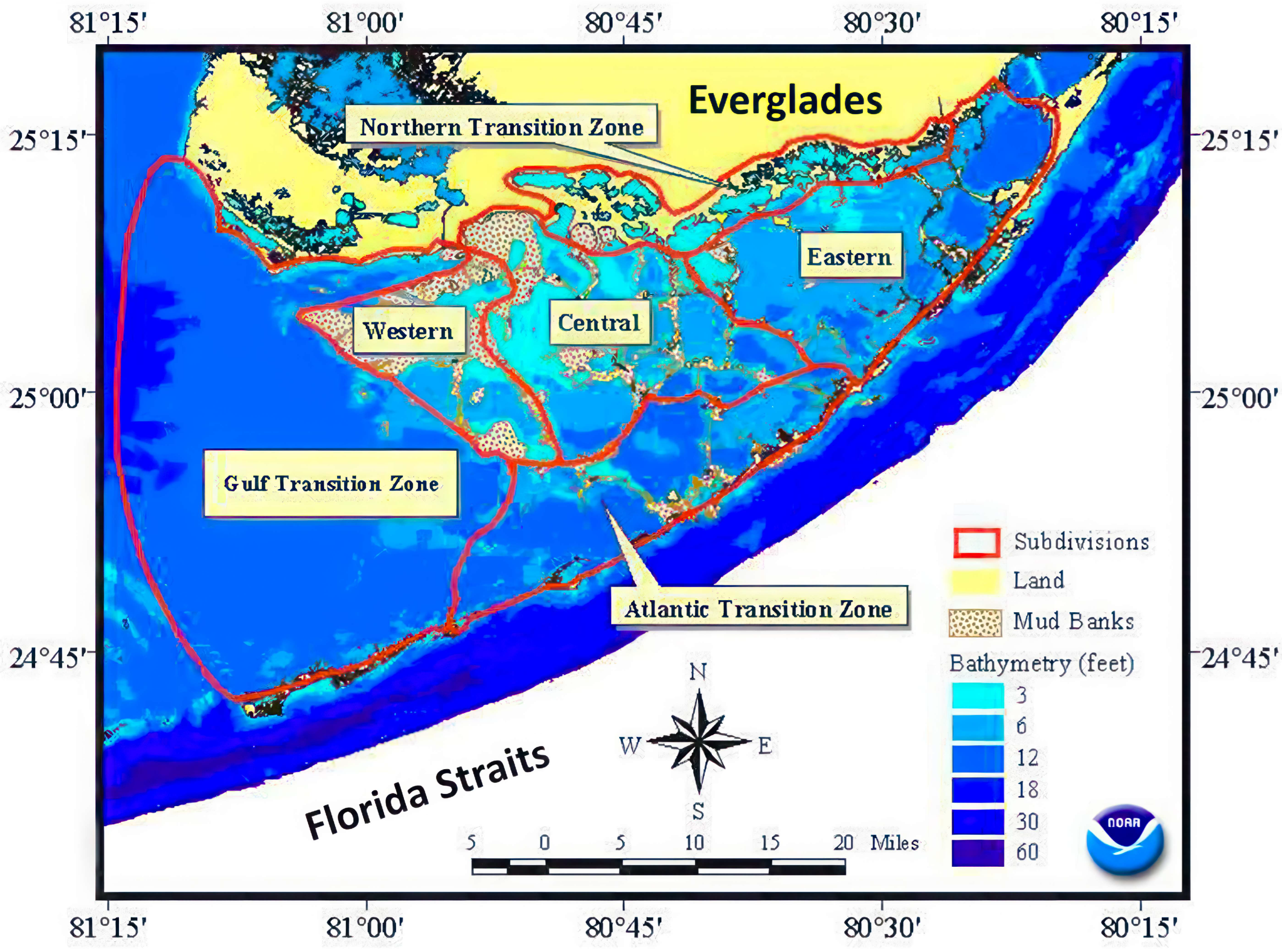
• Florida Bay exhibits a shift in the tidal regime, transitioning from macro-tidal in the western region to micro-tidal in the central and eastern/northeast regions. Shallow water depth (less than 1 m on average) and complex banks and shoals attenuate tides. Local winds and the subtidal variations from the Gulf of Mexico and the Florida Straits are the primary drivers for the hydrodynamic processes in the eastern and central regions.
• Salinity changes in the bay, both temporally and spatially, are primarily controlled by three processes: the net supply of freshwater, the processes that drive mixing within the estuary (e.g., wind, topography, currents), and the exchange of salinity with the coastal ocean.
• Open boundary conditions from another ocean model with a larger domain (HYCOM in this study) can be adequate for simulating low-frequency sea level variability and salinity in the interior of Florida Bay when observational wind forcing fields are utilized.
• Grid sensitivity tests revealed that two vertical layers are necessary to simulate the bay. The use of four vertical layers and/or the fine horizontal grid did not significantly improve model accuracy.

The hydrodynamic model developed in this study has been coupled with a water quality model of Florida Bay, providing a comprehensive tool for supporting bay management [41].

References

- Ji, Z.-G. Hydrodynamics and Water Quality: Modeling Rivers, Lakes, and Estuaries, 2nd ed.; JohnWiley & Sons, Inc.: Hoboken, NJ, USA, 2017. [Google Scholar]
- Ganju, N.K.; Brush, M.J.; Rashleigh, B.; Aretxabaleta, A.L.; Del Barrio, P.; Grear, J.S.; Harris, L.A.; Lake, S.J.; McCardell, G.; O’Donnell, J.; et al. Progress and challenges in coupled hydrodynamic-ecological estuarine modeling. Estuaries Coasts 2016, 39, 311–332. [Google Scholar] [CrossRef]
- Iglesias, I.; Bio, A.; Melo, W.; Avilez-Valente, P.; Pinho, J.; Cruz, M.; Gomes, A.; Vieira, J.; Bastos, L.; Veloso-Gomes, F. Hydrodynamic model ensembles for climate change projections in estuarine regions. Water 2022, 14, 1966. [Google Scholar] [CrossRef]
- Iglesias, I.; Avilez-Valente, P.; Bio, A.; Bastos, L. Modelling the main hydrodynamic patterns in shallow water estuaries: The Minho Case Study. Water 2019, 18, 1040. [Google Scholar] [CrossRef]
- Hein, S.S.; Sohrt, V.; Nehlsen, E.; Strotmann, T.; Fröhle, P. Tidal Oscillation and Resonance in Semi-Closed Estuaries—Empirical Analyses from the Elbe Estuary, North Sea. Water 2021, 13, 848. [Google Scholar] [CrossRef]
- Zhang, M.L.; Zhu, X.S.; Wang, Y.J.; Jiang, H.Z.; Cui, L. A numerical study of hydrodynamic characteristics and hydrological processes in the coastal wetlands during extreme events. J. Hydrodyn. 2023, 35, 963–979. [Google Scholar] [CrossRef]
- Rudnick, D.T.; Ortner, P.B.; Browder, J.A.; Davis, S.M. A conceptual ecological model of Florida Bay. Wetlands 2005, 25, 870–883. [Google Scholar] [CrossRef]
- Wachnicka, A.; Gaiser, E.; Collins, L.; Frankovich, T.; Boyer, J. Distribution of diatoms and development of diatom-based models for inferring salinity and nutrient concentrations in Florida Bay and adjacent coastal wetlands of south Florida (USA). Estuaries Coasts 2010, 33, 1080–1098. [Google Scholar] [CrossRef]
- Kelble, C.R.; Johns, E.M.; Nuttle, W.K.; Lee, T.N.; Smith, R.H.; Ortner, P.B. Salinity patterns of Florida Bay. Estuar. Coast. Shelf Sci. 2007, 71, 318–334. [Google Scholar] [CrossRef]
- Lotze, H.K.; Lenihan, H.S.; Bourque, B.J.; Bradbury, R.H.; Cooke, R.G.; Kay, M.C.; Kidwell, S.M.; Kirby, M.X.; Peterson, C.H.; Jackson, J.B.C. Depletion, degradation, and recovery potential of estuaries and coastal seas. Sci. Mag. 2006, 312, 1806–1809. [Google Scholar] [CrossRef] [PubMed]
- McLean, A.R.; Ogden, J.C.; Williams, E.E. Comprehensive Everglades Restoration Plan; South Florida Water Management District: West Palm Beach, FL, USA, 2002.
- LoSchiavo, A.J.; Best, R.G.; Burns, R.E.; Gray, S.; Harwell, M.C.; Hines, E.B.; McLean, A.R.; St Clair, T.; Traxler, S.; Vearil, J.W. Lessons learned from the first decade of adaptive management in comprehensive Everglades restoration. Ecol. Soc. 2013, 18, 70. [Google Scholar] [CrossRef]
- D’Acunto, L.E.; Pearlstine, L.; Haider, S.M.; Hackett, C.E.; Shinde, D.; Romañach, S.S. The Everglades vulnerability analysis: Linking ecological models to support ecosystem restoration. Front. Ecol. Evol. 2023, 11, 1111551. [Google Scholar] [CrossRef]
- McAdory, R.T.; Kim, K.W. Field and Model Studies in Support of the Evaluation of Impacts of the C-111 Canal on Regional Water Resources, South Florida, Part IV: Florida Bay Hydrodynamic Modeling; US Army Corps of Engineers, Waterways Experiment Station: Vicksburg, MS, USA, 1998.
- Cerco, C.F.; Bunch, B.W.; Teeter, A.M.; Dortch, M.S. Water Quality Model of Florida Bay; Technical Report ERDC/EL TR-00-10; U.S. Army Corps of Engineers: Vicksburg, MS, USA, 2000.
- Wang, J.D.; van de Kreeke, J.; Krishnan, N.; Smith, D. Wind and Tide Response in Florida Bay. Bull. Mar. Sci. 1994, 54, 579–601. [Google Scholar]
- Wang, J.D. Subtidal Flow Patterns in Western Florida Bay. Estuar. Coast. Shelf Sci. 1998, 46, 901–915. [Google Scholar] [CrossRef]
- Sheng, Y.P.; Davis, J.R.; Liu, Y. A Preliminary Model of Florida Bay Circulation; Final Report to the National Park Service; University of Florida: Gainesville, FL, USA, 1995. [Google Scholar]
- Hamrick, J.M. A Three-Dimensional Environmental Fluid Dynamics Computer Code: Theoretical and Computational Aspects; Special Report 317; The College of William and Mary, Virginia Institute of Marine Science: Gloucester Point, VA, USA, 1992; 63p. [Google Scholar]
- Hamrick, J.M. Users Manual for the Environmental Fluid Dynamic Computer Code; Special Report 328; The College of William and Mary, Virginia Institute of Marine Science: Gloucester Point, VA, USA, 1996; 224p. [Google Scholar]
- Mellor, G.L.; Yamada, T. Development of a turbulence closure model for geophysical fluid problems. Rev. Geophys. Space Phys. 1982, 20, 851–875. [Google Scholar] [CrossRef]
- Galperin, B.; Kantha, L.H.; Hassid, S.; Rosati, A. A quasi-equilibrium turbulent energy model for geophysical flows. J. Atmos. Sci. 1988, 45, 55–62. [Google Scholar] [CrossRef]
- Ji, Z.G.; Morton, M.R.; Hamrick, J.M. Wetting and drying simulation of estuarine processes. Estuar. Coast. Shelf Sci. 2001, 53, 683–700. [Google Scholar] [CrossRef]
- Ji, Z.-G.; Hamrick, J.H.; Pagenkopt, J. Sediment and metals modeling in shallow river. J. Environ. Eng. 2002, 128, 105–119. [Google Scholar] [CrossRef]
- Ji, Z.-G.; Jin, K.R. Gyres and seiches in a large and shallow lake. J. Great Lakes Res. 2006, 32, 764–775. [Google Scholar] [CrossRef]
- Ji, Z.G.; Hu, G.; Shen, J.; Wan, Y. Three-dimensional modeling of hydrodynamic processes in the St. Lucie Estuary. Estuar. Coast. Shelf Sci. 2007, 73, 188–200. [Google Scholar] [CrossRef]
- Ji, Z.-G.; Jin, K.R. An integrated environmental model for a surface flow constructed wetland: Water quality processes. Ecol. Eng. 2016, 86, 247–261. [Google Scholar] [CrossRef]
- Tetra Tech, Inc. Florida Bay Hydrodynamic and Salinity Model Analysis; South Florida Water Management District: Fairfax, VA, USA, 2003; 92p.
- Tetra Tech, Inc. Development of a Florida Bay and Florida Keys Hydrodynamic and Water Quality Model: Grid Resolution Analysis; South Florida Water Management District: Fairfax, VA, USA, 2004; 137p.
- Langevin, C.D.; Swain, E.D.; Wang, J.D.; Wolfert, M.A.; Schaffranek, R.W.; Riscassi, A.L.; Bay, F. Development of Coastal Flow and Transport Models in Support of Everglades Restoration; US Geological Survey Fact Sheet 3130; US Geological Survey: Reston, VA, USA, 2004; pp. 3–6.
- U.S. Environmental Protection Agency. Technical Guidance Manual for Performing Waste Load Allocations, Book III Estuaries, Part 2, Application of Estuarine Waste Load Allocation Models; EPA 823-R-92-003; U.S. Environmental Protection Agency: Washington, DC, USA, 1990.
- Marsaleix, P.; Auclair, F.; Estournel, C. Considerations on open boundary conditions for regional and coastal ocean models. J. Atmos. Ocean. Technol. 2006, 23, 1604–1613. [Google Scholar] [CrossRef]
- Diederen, D.; Savenije, H.H.G.; Toffolon, M. The open boundary equation. Ocean Sci. Discuss. 2015, 12, 925–958. [Google Scholar]
- Liu, Z.; Gan, J. A modeling study of estuarine–shelf circulation using a composite tidal and subtidal open boundary condition. Ocean Model. 2020, 147, 101563. [Google Scholar] [CrossRef]
- Bleck, R. An oceanic general circulation model framed in hybrid isopycnic-cartesian coordinates. Ocean Modell. 2002, 37, 55–88. [Google Scholar] [CrossRef]
- Olvera-Prado, E.R.; Romero-Centeno, R.; Zavala-Hidalgo, J.; Moreles, E.; Ruiz-Angulo, A. Contribution of the wind, Loop Current Eddies, and topography to the circulation in the southern Gulf of Mexico. Ocean Dyn. 2023, 73, 597–618. [Google Scholar] [CrossRef]
- Andrejev, O.; Soomere, T.; Sokolov, A.; Myrberg, K. The role of the spatial resolution of a three-dimensional hydrodynamic model for marine transport risk assessment. Oceanologia 2011, 53, 309–334. [Google Scholar] [CrossRef]
- Hasan, G.J.; van Maren, D.S.; Cheong, H.F. Improving hydrodynamic modeling of an estuary in a mixed tidal regime by grid refining and aligning. Ocean Dyn. 2012, 62, 395–409. [Google Scholar] [CrossRef]
- Ralston, D.K.; Cowles, G.W.; Geyer, W.R.; Holleman, R.C. Turbulent and numerical mixing in a salt wedge estuary: Dependence on grid resolution, bottom roughness, and turbulence closure. J. Geophys. Res. Ocean. 2017, 122, 692–712. [Google Scholar] [CrossRef]
- Nwogwu, N.A.; Linhoss, A.C.; Alarcon, V.J.; Mickle, P.F.; Kelble, C.R. The Effect of grid resolution on hydrodynamic modeling of estuarine water surface elevation: Balancing efficiency and accuracy. In Proceedings of the OCEANS 2023-MTS/IEEE US Gulf Coast, Biloxi, MS, USA, 25–28 September 2023; pp. 1–10. [Google Scholar]
- Moustafa, M.Z.; Ji, Z.-G. Impacts of freshwater sources on salinity structure in a large, shallow estuary. Environments, 2024; submitted. [Google Scholar]