Diffusion Characteristics and Mechanisms of Thermal Plumes from Coastal Power Plants: A Numerical Simulation Study

Abstract

Plumes include thermal plumes and cold plumes, of which thermal plumes receive more attention. Thermal plumes refer to the formation of high-temperature fluid structures near a heat source, which diffuse and propagate within the surrounding environment. In this study, we simulate the formation and evolution of thermal plumes using numerical modeling. Taking Wushashan Power Plant in Xiangshan Bay as an example, the diffusion characteristics of the thermal plume near the power plant were simulated by the optimized FVCOM. Combined with statistical methods and advanced mathematical models, the plume diffusion range under different working conditions was quantified, and the diffusion mechanism was studied. For example, we found that when the flow velocity is halved, the diffusion area of the surface thermal plume decreases by more than half. When the flow rate in Xiangshan Bay is reduced to 5 m³/s, the area of surface temperature rise plumes is small. Using the Richardson number, the characteristics and mechanisms of stratification/mixing near the power plant were explored. It was found that the flow field near the power plant was mainly affected by the momentum of the outlet. During a typhoon, the wind strength and path impact thermal plume diffusion via wind-driven flow.

1. Introduction

The impact of sea temperature and thermal discharge on marine ecology has been an important issue in the fields of oceanography and environmental protection. Previous studies on sea temperature and thermal discharge in bays have primarily focused on on-site measurements [1], physical modeling, remote sensing measurements [2], and numerical simulations [3]. On-site observations involve continuous monitoring at multiple points, combining meteorological, water level, and ocean current data to analyze the distribution of and variations in thermal discharge, as well as discuss the main influencing factors [4]. Based on field observations, Zhao studied the temporal and spatial distribution characteristics of winter thermal discharge in Sanmen Bay, and found that the south of Sanmen Bay was more affected by thermal discharge during the neap tide period [5]. Based on a field investigation, Li analyzed the aquaculture scale and the water environment of the sea area before and after the operation of the power plant. While on-site observations provide high accuracy, they are costly, time-consuming, and often cannot capture large-scale spatial distributions; hence, they are rarely conducted as standalone studies.

Physical modeling is a useful approach for simulating the three-dimensional flow, buoyancy effects, and mixing of thermal discharges in the vicinity of discharge outlets. Researchers both in China and internationally have conducted numerous studies on the impact of thermal discharge from power plants on adjacent marine environments [6]. For example, the effects of thermal discharge from power plants such as the two power plants in the vicinity of the Yangtze River estuary, Xinhuai Power Plant and Daya Bay Nuclear Power Plant, have been analyzed based on physical modeling [7,8]. Based on the physical model of thermal discharge, Wang compared and analyzed the changes in water temperature rise and the characteristics of the temperature field in the nearby area under different schemes [9]. Liang built a three-dimensional physical model of thermal discharge, and found that the mixing effect of water flow near the outlet was strong [10]. However, the selection of physical models, comprehensive heat dissipation coefficients on water surfaces, and model scaling parameters can significantly affect the accuracy of the models.

Remote sensing observations have also been employed as an effective method for studying the dispersion of thermal discharge. AVHRR, MODIS, and Landsat remote sensing data have been widely used in sea surface temperature (SST) retrievals [11], which further enables the study of the diffusion range of thermal discharge [12,13,14]. Based on Landsat5 TM and HJ-1B, Xu studied the sea surface temperature and thermal discharge temperature rise near the Daya Bay nuclear power station, and compared the differences between the two sets of satellite data [15]. Yang used satellite remote sensing technology to detect five-year satellite remote sensing data and analyzed the impact of thermal discharge on aquaculture areas in coastal waters [16]. The study of thermal discharge often requires the retrieval of nearshore SST using remote sensing data. However, due to spatial resolution limitations [17], remote sensing usually requires a combination with numerical models or on-site observations [18].

Numerical simulation is an important tool in studying the thermal dynamics of rivers and nearshore areas [19,20]. Scholars began with two-dimensional simulations [21], using unstructured grids for grid refinement and simulating the diffusion characteristics and patterns of thermal discharge under different conditions, such as the Qiongzhou Strait power plant and the Zhangzhou Houshi power plant [21,22]. However, two-dimensional simulations, which are based on vertically averaged simulations, have significant limitations in predicting results [23,24]. Through comparative studies involving two-dimensional and three-dimensional simulations and flume experiments, it has been found that three-dimensional models perform better than two-dimensional models in capturing the three-dimensional characteristics of buoyant jets and the driving effect of momentum [25]. In recent years, scholars have used three-dimensional models to explore the diffusion patterns of thermal discharge. For example, the numerical results of three-dimensional thermal discharge diffusion at a nuclear power plant in western South Korea demonstrated that intertidal flats significantly affect the dispersion of thermal discharge [26]. The horizontal distribution of temperature fields caused by thermal discharge is influenced by the combined effects of tidal flow and water depth topography, and the “temperature jump” phenomenon is caused by the offshore jet of high-temperature seawater during specific moments [27]. Factors such as the estuaries, lagoons, and harbors near discharge outlets, as well as discharge volume, are key factors influencing thermal plumes, and wind also has a significant impact [28]. This research employs numerical experiments to investigate the effects of essential factors, such as thermal discharge rate, Coriolis force, and discharge outlet location, on the thermal discharge from thermal plumes. Through these experiments, a comprehensive understanding of the dispersion patterns and mechanisms of thermal plumes is achieved, providing valuable insights for marine environmental management and engineering design.

In this study, a three-dimensional ocean numerical model (FVCOM) and high-resolution bathymetric data were used to accurately establish a temperature rise plume diffusion model by taking the thermal discharge in a semi-enclosed bay as an example. On the basis of accurate model verification, different experimental conditions were designed to explore the diffusion law and mechanisms of the plume under different weather conditions, different flow rates, and different discharge modes, which can supplement the previous research on thermal discharge plumes. The results of this study provide an important scientific basis for marine engineering construction and environmental protection, and help to optimize the design of drainage systems, reduce potential adverse effects on the marine environment, and support the sustainable development of coastal areas and the protection of marine ecosystems.

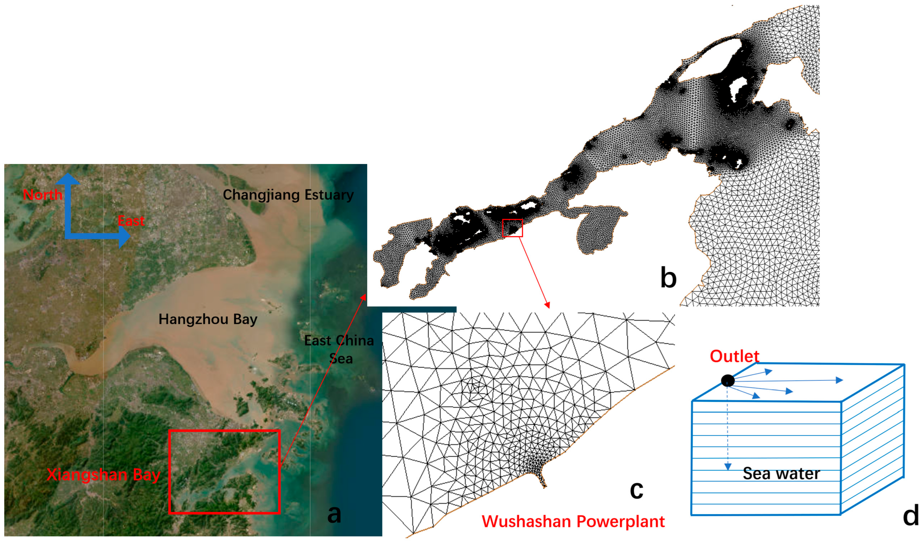
2. Description of Study Area and Thermal Discharge

Xiangshan Bay is a strong tidal bay with distinct climatic seasons. When tidal waves from the open sea enter the bay, they gradually transition from progressive waves to standing waves. Influenced by the terrain and land boundaries, a reciprocating flow pattern is observed, with the direction basically parallel to the shoreline. The annual average temperature is 16.2–17.0 °C, with an average annual sunlight duration of 1904–1999 h and an average annual precipitation of 1239–1522 mm [29]. There are two relatively dry and wet seasons throughout the year: March to June and September are the relatively wet seasons, while July to August and October to next February are the relatively dry seasons. The annual evaporation is 1417–1503 mm. The average annual wind speed is 3.8 m/s. From September to the following March, the dominant winds are from the northwest and west, while from April to August, the winds are primarily from the southeast and south. The average annual occurrence rate of calm wind is 11%. The average water temperature in Xiangshan Bay is about 16.4 °C. The hottest month is August, with an average temperature of 26.5–27.0 °C. The coldest month is January, with an average temperature between 3.0 and 7.2 °C [29].

Xiangshan Bay includes Ninghai Power Plant and Wushashan Power Plant. In order to carry out detailed research, we take Wushashan Power Plant as an example. The intake of Wushashan Power Plant is located on the northern side of the plant area, within the waters of Xiangshan Bay. Its discharge outlet is on the western side of the power plant. It employs the open, shallow, and clear-channel discharge method for thermal discharge [17]. However, thermal discharge does have certain effects on water quality and temperature, thus necessitating continuous monitoring and management to protect the bay’s ecological environment.

3. Model Configuration and Verification

In the horizontal direction, the FVCOM model employs unstructured triangular grids, while in the vertical direction, it utilizes a σ-coordinate transformation [30], enabling a more accurate simulation of complex coastlines and seabed topography.

Continuity equation:

$$\frac{\partial \zeta }{\partial t}+\frac{\partial Du}{\partial x}+\frac{\partial Dv}{\partial y}+\frac{\partial w}{\partial \sigma }=0$$

(1)

Momentum equation:

$$\begin{array}{c}\frac{\partial uD}{\partial t}+\frac{\partial u^{2}D}{\partial x}+\frac{\partial uvD}{\partial y}+\frac{\partial uw}{\partial \sigma }-fvD=-gD\frac{\partial \zeta }{\partial x}\\ -\frac{g}{{\rho }_0}\left[\frac{\partial }{\partial x}\left(D{\int }_{\sigma }^0\rho d\sigma \prime \right)+\sigma \rho \frac{\partial D}{\partial x}\right]+\frac{1}{D}\frac{\partial }{\partial \sigma }\left(K_m\frac{\partial u}{\partial \sigma }\right)+D{F}_x\end{array}$$

(2)

$$\begin{array}{c}\frac{\partial vD}{\partial t}+\frac{\partial uvD}{\partial x}+\frac{\partial v^{2}D}{\partial y}+\frac{\partial vw}{\partial \sigma }+fuD=-gD\frac{\partial \zeta }{\partial y}\\ -\frac{gD}{{\rho }_0}\left[\frac{\partial }{\partial y}\left(D{\int }_{\sigma }^0\rho d\sigma \prime \right)+\sigma \rho \frac{\partial D}{\partial y}\right]+\frac{1}{D}\frac{\partial }{\partial \sigma }\left(K_m\frac{\partial v}{\partial \sigma }\right)+D{F}_y\end{array}$$

(3)

$$\begin{array}{c}\frac{\partial TD}{\partial t}+\frac{\partial TuD}{\partial x}+\frac{\partial TvD}{\partial y}+\frac{\partial Tw}{\partial \sigma }=\frac{1}{D}\frac{\partial }{\partial \sigma }\left(K_h\frac{\partial T}{\partial \sigma }\right)+D\widehat{H}+D{F}_T\end{array}$$

(4)

$$\frac{\partial SD}{\partial t}+\frac{\partial SuD}{\partial x}+\frac{\partial SvD}{\partial y}+\frac{\partial Sw}{\partial \sigma }=\frac{1}{D}\frac{\partial }{\partial \sigma }\left(K_h\frac{\partial S}{\partial \sigma }\right)+D{F}_S$$

(5)

$$\begin{array}{c}\rho =\rho (T,S)\end{array}$$

(6)

In the equation above, C is a constant. $P_r$ denotes the Prandtl number. f is the Coriolis force parameter, ρ is the density of seawater, u and v represent horizontal velocity components, w is vertical velocity, and t represents time. $\zeta$ is water level, and z represents the vertical coordinate. $z=\zeta (x,y,t)$ represents the sea surface, and $z=H(x,y)$ represents the seabed. $A_h$ is the horizontal eddy thermal diffusion coefficient, $A_m$ is the viscosity coefficient of horizontal vortex, $K_m$ is the vertical eddy viscosity coefficient, and $K_h$ is the vertical rotational diffusion coefficient of heat. $q^2$ is the turbulent kinetic energy, and $l$ is the turbulent mixing length. The horizontal mixing calculation of the hydrodynamic model adopts the Smagorinsky turbulence closure scheme. The Mellor–Yamada level 2.5-order turbulence closure scheme is used for vertical mixing calculation [30]. $\widehat{H}$ represents the solar radiation absorbed by water bodies. $F_T,F_S$ represent the horizontal diffusion terms of temperature and salinity, respectively.

The boundary of the island or coastline represents the closed boundary, and the node velocity on the closed boundary is 0. Therefore, the kinematic boundary conditions at the closed boundary are

$$\begin{array}{c}{v}_n=0\end{array}$$

(7)

Here, n is the normal coordinate axis of the boundary, and v is the normal velocity component of the boundary.

On the free surface,

$$\begin{array}{c}\left(\frac{\partial u}{\partial \sigma },\frac{\partial v}{\partial \sigma }\right)=\frac{D}{{\rho }_0{K}_m}({\tau }_{sx},{\tau }_{sy})\end{array}$$

(8)

${\tau }_{sx}$ and ${\tau }_{sy}$ are the components of surface wind stress in two horizontal directions, respectively.

At the bottom,

$$\begin{array}{c}\left(\frac{\partial u}{\partial \sigma },\frac{\partial v}{\partial \sigma }\right)=\frac{D}{{\rho }_0{K}_m}({\tau }_{bx},{\tau }_{by})\end{array}$$

(9)

${\tau }_{bx}$ and ${\tau }_{by}$ are the components of surface wind stress in two horizontal directions, respectively.

Based on the actual environment of Xiangshan Bay and model experience, the basic model was established. Harmonic constants for 13 tidal constituents (M₂, S₂, N₂, K₂, K₁, O₁, P₁, Q₁, M_f, M_m, M₄, MS₄, MN₄) at the open boundary grid nodes were obtained through interpolation from the TPXO global tidal model, and water levels at the open boundaries during the model run were obtained using tidal harmonic analysis [31]. The open boundary of the model avoided islands in order to prevent boundary effects. The wet–dry grid processing module was enabled to assess tidal flat exposure and inundation conditions. The sea floor roughness height and other parameters in the model ere set according to the literature [32]. The model employs a cold start, with initial flow velocities, tidal levels, and so on set to zero. The open boundary and initial temperature and salinity are based on HYCOM data (https://www.hycom.org/hycom, accessed on 1 September 2020). Due to the limited precision of HYCOM, interpolation was performed for the nearshore area. The external mode time step was set to 0.4 s, and the internal mode time step was set to 2 s. The external model of FVCOM is two-dimensional, and was used to calculate the water level and vertical average velocity. The internal model is three-dimensional, and was used to calculate the three-dimensional velocity, temperature, salinity, and turbulence parameters. Meteorological conditions such as air temperature, relative humidity, shortwave radiation, and wind speed are based on data from the European Centre for Medium-Range Weather Forecasts (https://www.ecmwf.int/). Because Xiangshan Bay is a narrow bay with poor water exchange, Wushashan Power Plant is located in the middle of the bay, and the Yangtze River and Qiantang River are relatively far away, the bay is less affected by the two big rivers, and their influence was ignored here. This paper focused on the study of seawater temperature and heat, so the influence of salinity was not considered.

The grid boundary was set in the East China Sea area with a spatial resolution of about 30 km. In order to improve the accuracy of the simulation calculations in Xiangshan Bay, the grid was increased inside the bay. The resolution of neighboring Xiangshan Bay was refined to 2 km, and the grid resolution gradually increased from about 500 m at the entrance to the bay. The grid resolution near the drainage outlet and islands reached 15 m. In order to accurately simulate the actual drainage outlet, special treatment was carried out near the power plant drainage outlet, adding channels for the drainage outlet, and the grid was presented in a radial shape. The research area was divided into 119,121 units with 63,091 nodes, and the seawater was vertically divided into 10 layers.

Based on the actual discharge methods of thermal discharge within the bay, we established the diffusion model within the bay. Wushashan Power Plant (Figure 1) has its water intake on the north side of Xiangshan Bay, with the discharge outlet located on the west side of the power plant.

The power plant discharge was simulated with a constant-flow-rate method. In order to align with actual conditions, the water was drawn from the bottom layer of the shore closest to the water intake, the water intake volume was consistent with the discharge volume, and the temperature and salinity of the water intake were set to match those at the actual intake point far from the nearshore. Wushashan Power Plant discharges heated wastewater at a rate of 82.0m³/s, with a temperature increase of 8.5 °C.

The verification of hydrodynamics involved tidal level, flow velocity, and flow direction. Furthermore, this study validated the storm surge and tidal level during typhoon weather conditions. The seawater temperature was verified at multiple fixed stations, encompassing different layers of the ocean. In addition, the sea surface temperature (SST) within the bay was retrieved using Landsat satellite data. A comparison was made between the retrieved SST and the simulated SST to demonstrate the accuracy of the seawater temperature simulation. For verification of hydrodynamics and thermodynamics, please refer to our previously published paper [33].

4. Analysis of Thermal Plume Characteristics

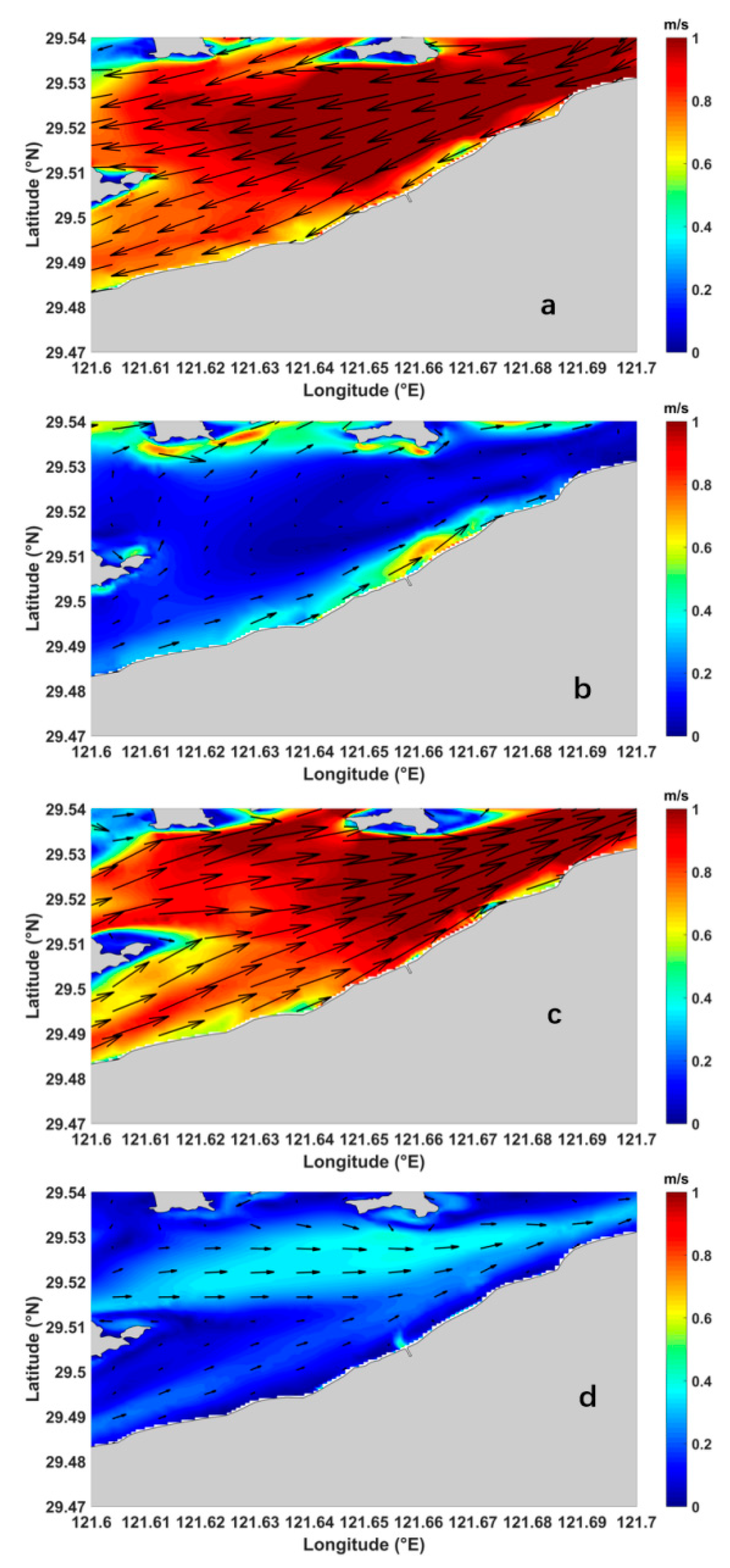
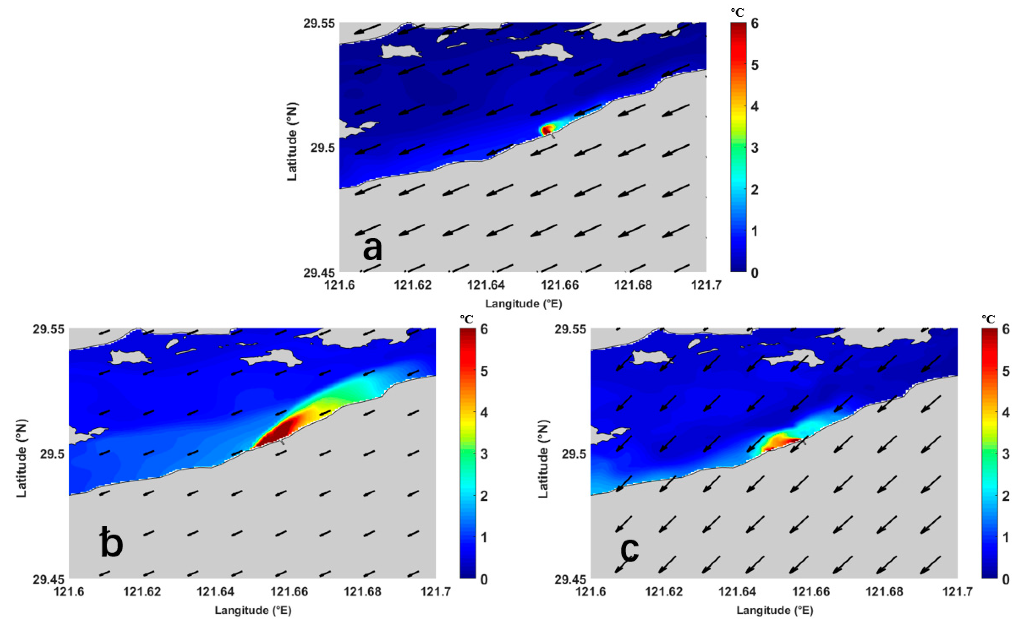
4.1. Flow Field near Wushashan Power Plant

Under the influence of the narrow shape of Xiangshan Bay and numerous islands, the tidal distribution exhibits an asymmetric pattern within the bay and around the islands. The tidal range gradually increases from the bay entrance to the head of the bay. This section aims to explore the overall characteristics of the flow field in the bay, specifically near the outlet of the power plant, during spring and neap tides, in order to comprehend the variations in the flow field. Special attention is given to investigating the changes in the flow field near the two power plants. Taking spring tides as an example, this section presents the magnitude and direction of flow velocity during four tidal phases (Figure 2 and Figure 3).

By comparing the surface flow fields of the power plant during four tidal stages, it is evident that the flow velocities during flood rapid and ebb rapid moments are significantly higher than during flood slack and ebb slack moments. Specifically, the flow velocity near Wushashan Power Plant is large, which can be attributed to its location in the central part of the bay and the relatively narrow waterway in that area. The variation in flow velocity at the power plant discharge outlets is mainly influenced by the inherent flow field in the bay, particularly during periods of higher inherent flow velocity (peak flood and peak ebb), where this influence becomes more pronounced. Conversely, during periods of lower inherent flow velocity (high slack water and low slack water), there are areas of increased flow velocity near the discharge outlets. The flow velocity near Wushashan Power Plant exhibits a southwest–northeast direction, which is associated with the waterway direction near the power plant (Figure 1b,c). A comparison of the distribution of surface and bottom flow fields reveals that peak flood and peak ebb continue to exhibit higher flow velocities, with the overall flow velocity in the bottom layer being lower than that in the surface layer. There are no significant areas of increased flow velocity near the discharge outlets in the bottom layer during high slack water and low slack water, indicating a relatively minor influence of thermal discharge on the flow field in the bottom layer of the bay.

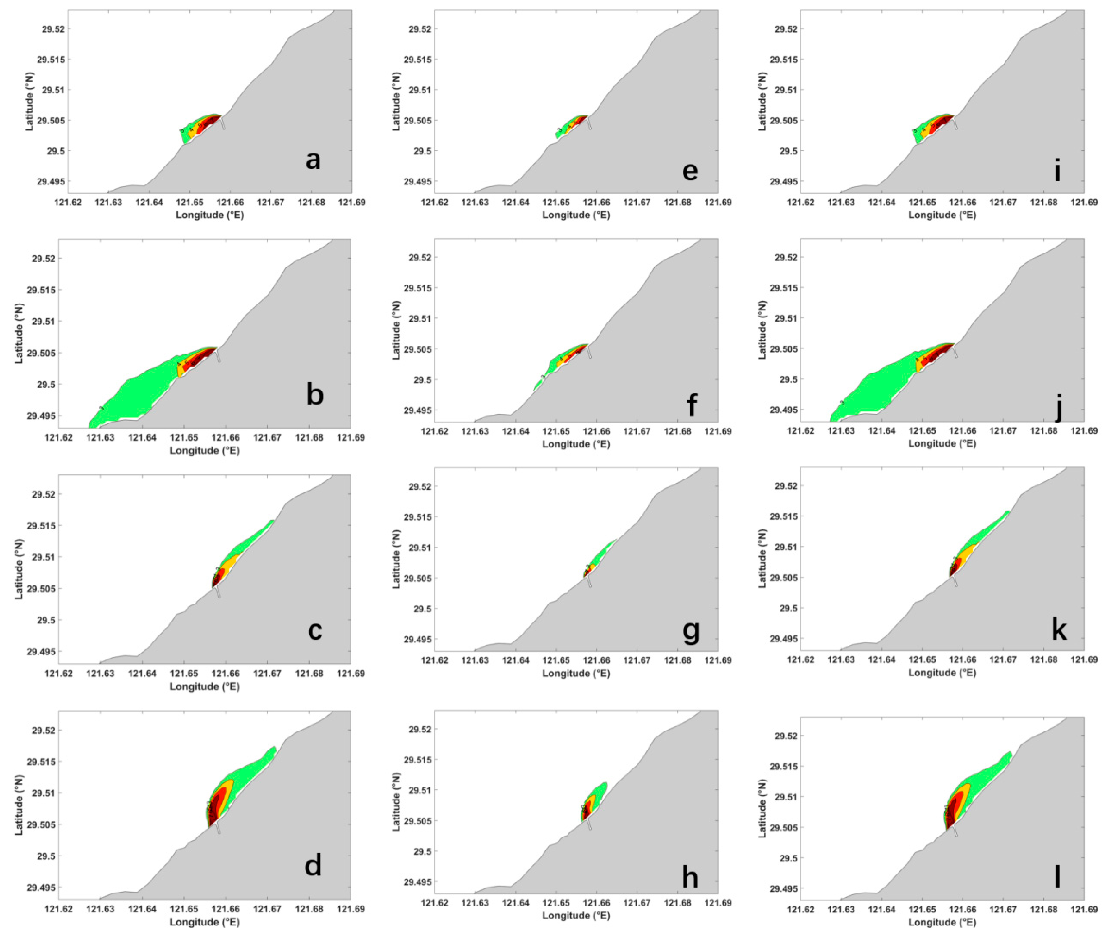
4.2. Dispersion Characteristics of Thermal Plume during Calm Weather and Typhoons

Under calm weather conditions, the dispersion characteristics of thermal plumes significantly impact the seawater temperature. Taking normal summer weather conditions as an example, experimental scenarios are set up. Exp1 serves as the control condition, while Exp2 investigates the influence of halved thermal discharge flow rates from the power plant on the temperature rise plume near the plant. Exp3 simulates the distribution of temperature fields without considering the Coriolis force, studying the variations in the temperature rise plume under the influence of the Coriolis force. Exp4 examines the changes in the temperature rise plume caused by bottom thermal discharge from the power plant, comparing and analyzing the effects of bottom and surface thermal discharge. Exp7 represents the scenario without thermal discharge. Exp5 and Exp6 are designed with lower flow rates to study the diffusion characteristics of the plume under low-flow conditions. The temperature fields obtained from Exp7 are subtracted from the temperature fields obtained from Exp1 to Exp6 to calculate the distribution of temperature rise under different conditions. Subtracting Exp7 from Exp1 reveals the distribution of temperature rise under normal thermal discharge flow rates, considering the Coriolis force and surface discharge. Similarly, subtracting Exp7 from Exp2 yields the temperature rise field under reduced flow rates, enabling the analysis of the influence of flow rates on plume dispersion. Subtracting Exp7 from Exp3 reveals the temperature rise field without considering the Coriolis force, allowing for an analysis of the impact of the Coriolis force on the plume. Subtracting Exp7 from Exp4 provides the distribution of temperature rise caused by bottom-level thermal discharge, facilitating the comparison and analysis of the effects of surface-level and bottom-level discharge on plume dispersion. Finally, subtracting Exp7 from Exp5 and Exp6 reveals the distribution of the plume under low-flow-rate conditions.

In the context of typhoon weather conditions, this study focuses on the Wushashan Power Plant and analyzes temperature rise plumes as the subject of investigation. Numerical experiments are designed to examine the influence of typhoon path and intensity on the extent of temperature rise plume dispersion, as illustrated in

Table 1. Experimental conditions.

Experimental Condition	Explanation
Exp1	Considering the Wushashan Power Plant, the flow rate was set at 82.5 m3/s, taking into account the Coriolis force and surface discharge during calm weather.
Exp2	On the basis of Exp1, but the flow rate of the power plant was halved.
Exp3	On the basis of Exp1, but the influence of the Coriolis force was not considered.
Exp4	On the basis of Exp1, but the thermal effluents were changed to bottom discharge.
Exp5	Surface discharge, considering the Coriolis force, with a flow rate of 10 m3/s from the power plant.
Exp6	Surface discharge, considering the Coriolis force, with a flow rate of 5 m3/s from the power plant.
Exp7	On the basis of Exp1, but the thermal effluents were not considered.
Exp8	The actual typhoon path and intensity of the Typhoon Lichima period, only considering the thermal discharge of Wushashan Power Plant.
Exp9	Based on Exp8, but typhoon intensity was halved.
Exp10	Based on Exp8, but the typhoon path moves north by 1 degree.
Exp11	Based on Exp8, but does not consider thermal discharge.
Exp12	Based on Exp8, but the intensity of typhoons is halved. Does not consider thermal discharge.
Exp13	Based on Exp8, but the typhoon path moves north by 1 degree, and it does not consider thermal discharge.

. By comparing the discrepancies between Exp8 and Exp11, the distribution of temperature rise fields under normal typhoon conditions is determined. Subtracting Exp12 from Exp9 reveals the distribution of temperature rise fields when the typhoon intensity is halved. Additionally, the difference between Exp10 and Exp13 provides insights into the distribution of temperature rise fields under varying typhoon paths.

These combined findings contribute to a comprehensive understanding of thermal plume dynamics and their response to both calm and typhoon weather conditions, thereby offering valuable guidance for marine environmental management and engineering design.

Numerical experimental conditions were designed as shown in Table 1 to investigate the impact of typhoon path and intensity on the spreading range of the temperature rise plume. By subtracting Exp11 from Exp8, the temperature rise distribution under normal typhoon conditions was obtained. The subtraction of Exp12 from Exp9 resulted in the temperature rise plume distribution when the typhoon intensity was reduced by half. The difference between Exp10 and Exp13 provided the temperature rise plume distribution under the influence of changes in the typhoon path.

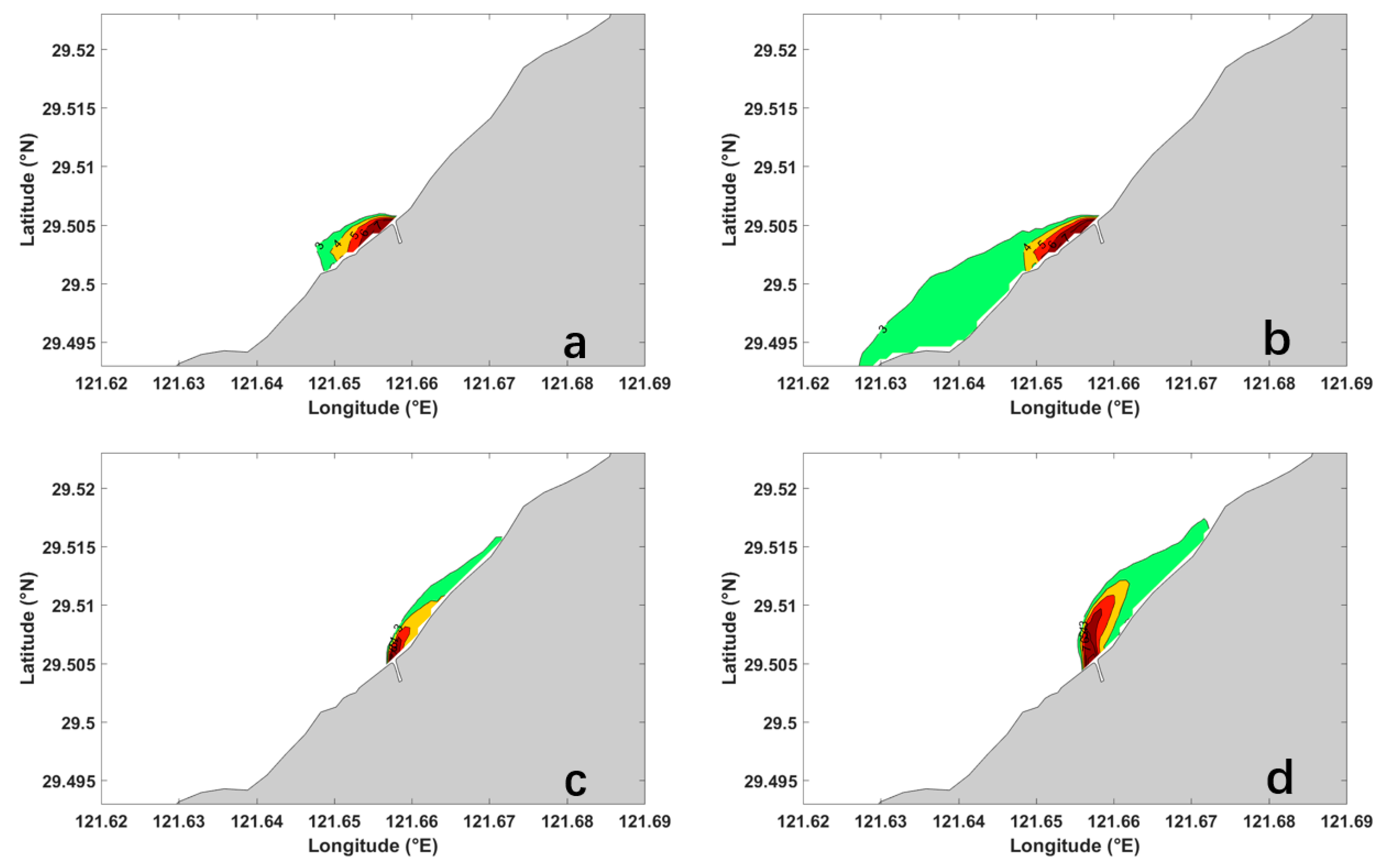
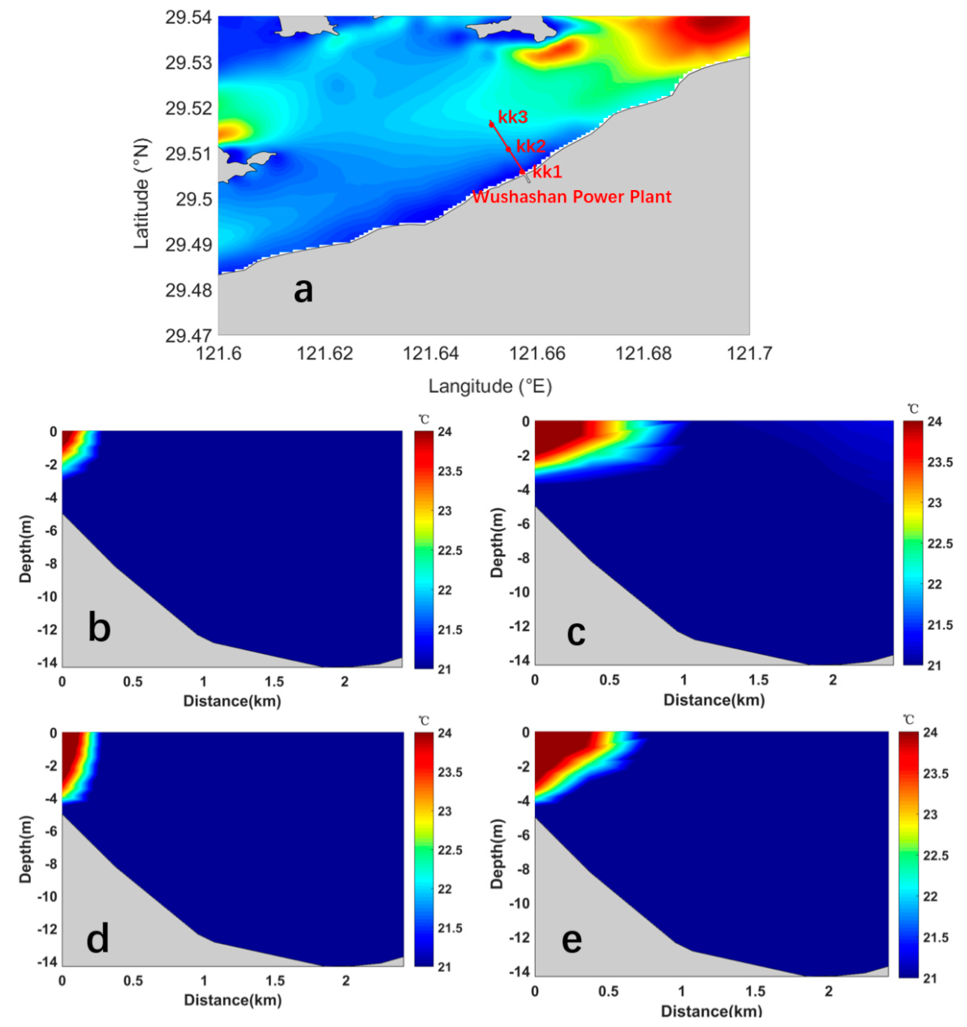
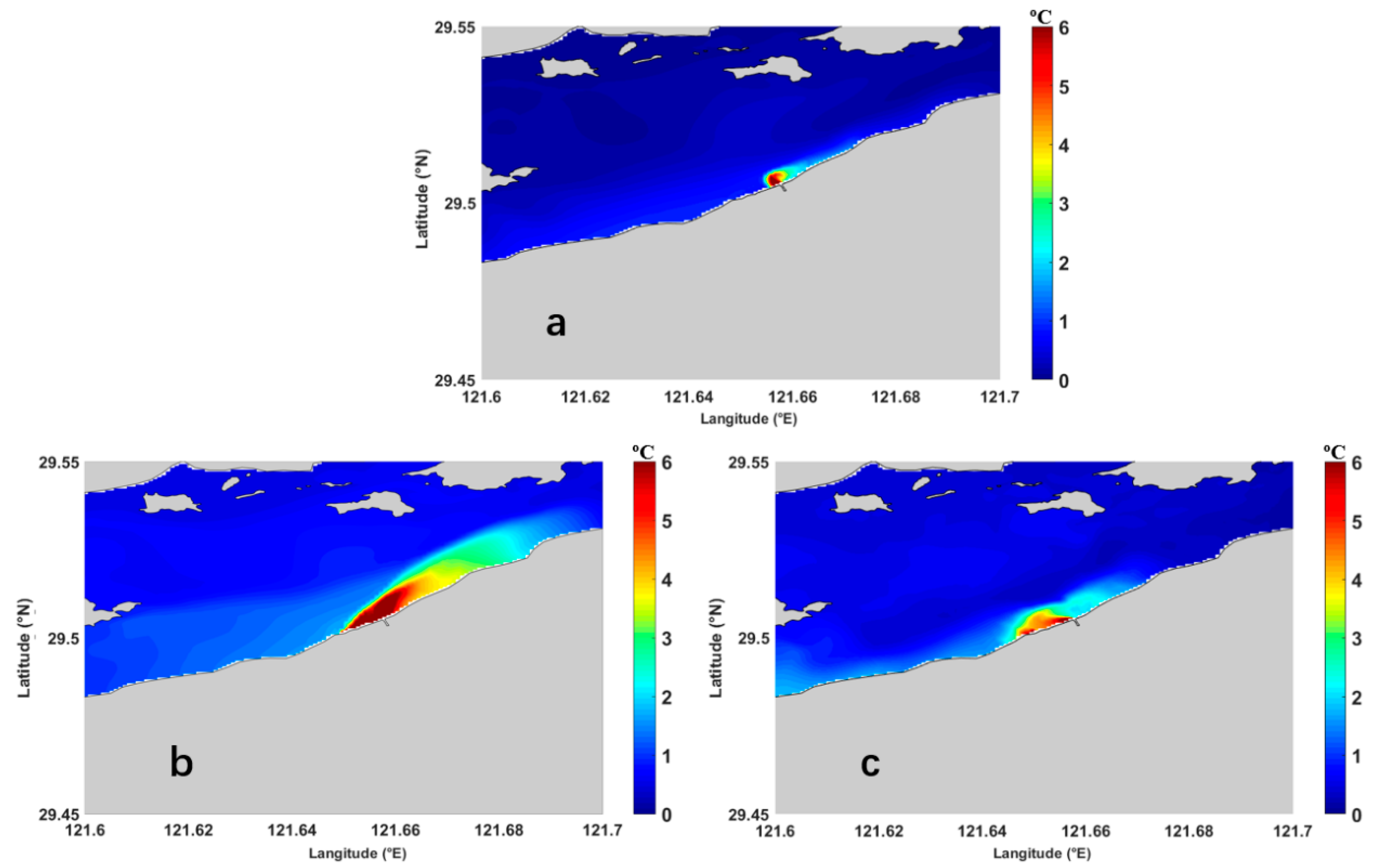
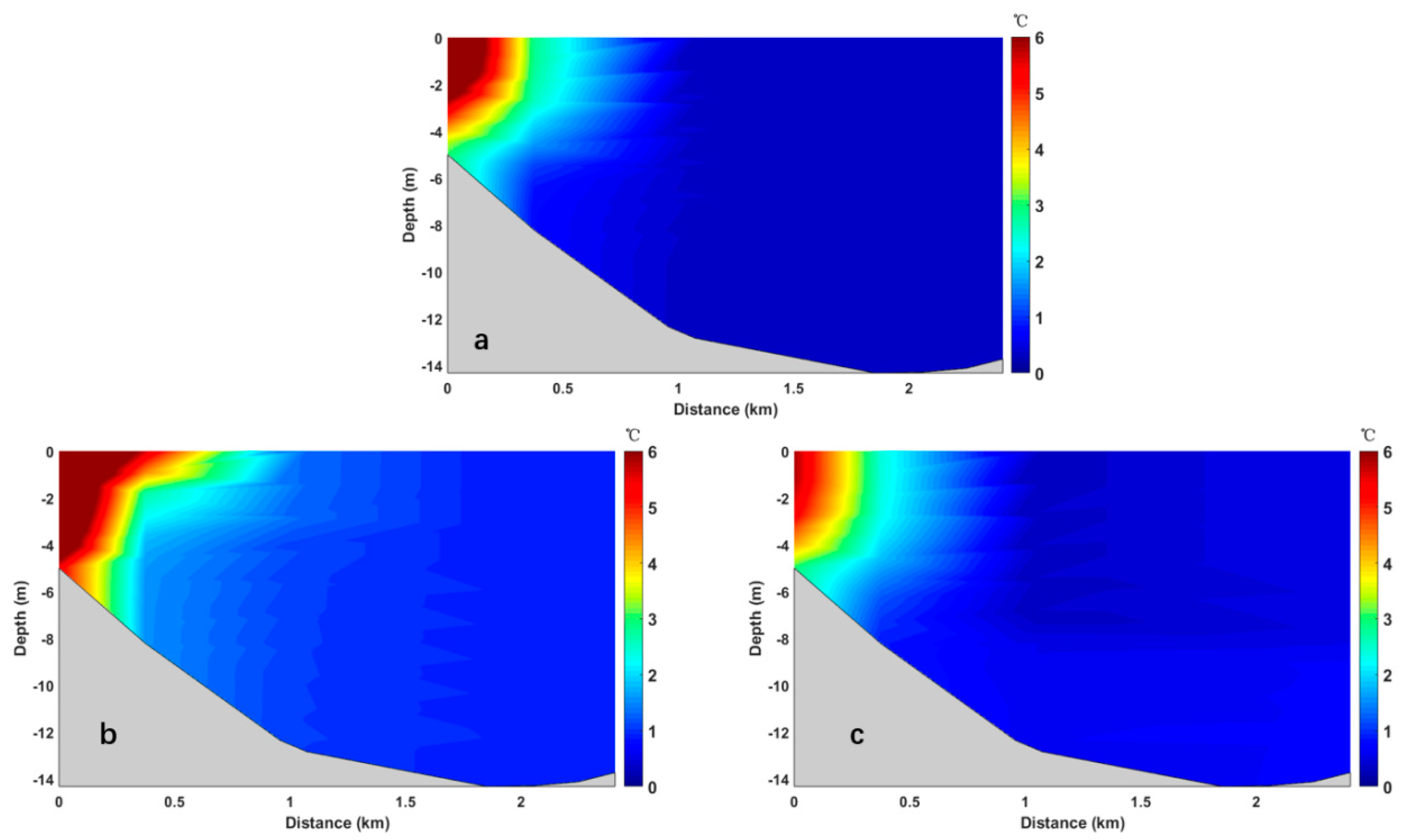
4.2.1. Analysis of Thermal Plume Characteristics

Based on Exp1 and Exp7, the horizontal spreading characteristics of the temperature rise plume flow were investigated under controlled conditions (Figure 4). Comparing the flow field near the power plant at corresponding times, it is found that the direction of the surface flow field of the seawater is basically consistent with the spreading direction of the temperature rise plume flow, indicating that the horizontal spreading direction of the plume flow is influenced by the flow field. The thermal discharge is significantly less strong than the natural flow within the bay, thus exerting no discernible impact on its inherent dynamics. Thermal plume flow is notably governed by convective control. Comparing the spreading ranges of the plume flow during the four tidal phases, it is found that the spreading range is the largest during slack water after a fall in ebb and slack water after rising floods. From the distribution of the flow field during these times, it can be seen that the flow velocity is small near Wushashan Power Plant during slack water after a fall in ebb and slack water after rising floods. The water flow discharged from the power plant outlet has a relatively higher velocity, making it easier to carry the temperature rise plume water to the offshore area and facilitating the spreading of the plume flow.

The Richardson number (Ri) was employed to quantify the mixing and stratification characteristics of the water surrounding the thermal plume flow [34].

$$Ri=-\frac{g}{\rho }\frac{\partial \rho }{\partial z}{(\frac{\partial u}{\partial z})}^{-2}$$

(10)

Here, ∂ρ and ∂u are estimated using the density difference (unit: kg/m³) and velocity difference (unit: m/s) of a specific water layer, while ∂z is approximately calculated using the water depth (unit: m) of that particular layer. ρ represents the vertically averaged density.

The density of water is primarily determined by temperature and salinity. In estuarine regions, pressure has a relatively minor effect on water density. When pressure is not considered, the density of seawater can be estimated using the formula provided by Geyer [35]:

$$\rho ={\rho }_w(1+\beta S_w)$$

(11)

In the above equation, β represents the salinity contraction coefficient (7.8 × 10⁻⁴). $S_w$ represents the salinity of the water, and ${\rho }_w$ represents the density of seawater. The calculation is performed using Bigg’s formula [36]:

$${\rho }_w=a_0+a_{1}t+a_2{t}^2+a_3{t}^3+a_4{t}^4+a_5{t}^5$$

(12)

Among them, a₀ is taken as 999.842594, a₁ is taken as 6.793952 × 10⁻², a₂ is taken as −9.095290 × 10⁻³, a₃ is taken as 1.001685 × 10⁻⁴, a₄ is taken as −1.12083 × 10⁻⁶, and a₅ is taken as 6.536332 × 10⁻⁹ [37].

Taking Wushashan Power Plant as an example, a representative cross-section H (Figure 5a) is selected, and the vertical temperature distribution of the water column is plotted during a tidal cycle (Figure 5b–e). The results show that the water temperature gradually decreases outward and downward along the cross-section from the discharge outlet of the power plant, indicating the presence of significant temperature gradients. Three characteristic points (kk1, kk2, kk3) are selected on the representative cross-section from the power plant outward (Figure 5a), and the Richardson number is calculated for these points at four tidal phases from the surface to the bottom. Ri is a dimensionless number that represents the ratio of potential energy to kinetic energy in the water column. For ease of presentation, the values of log₁₀(Ri/0.25) with respect to depth are plotted (Figure 6). Based on linear mixing theory, scholars [38,39] consider the critical value of Ri to be 0.25, where log₁₀(Ri/0.25) equals 0. When log₁₀(Ri/0.25) > 0, the water motion is stable, whereas when log₁₀(Ri/0.25) ≤ 0, the water column undergoes mixing.

From Figure 6, it can be observed that during the peak flood and peak ebb, the log₁₀(Ri/0.25) values at the kk2 and kk3 points are consistently smaller in all layers compared to the kk1 point. When comparing kk2 and kk3, it is evident that these points are located further away from the discharge outlet, and based on the vertical temperature distribution, the horizontal diffusion range of warm outflow is smaller during these two phases. Therefore, the points farther away are less influenced by the warm outflow. At the kk1 location, the overall trend of log₁₀(Ri/0.25) with water depth is initially increasing and then decreasing. This is due to the higher water temperature at the discharge outlet, transitioning to the region of temperature transition as depth increases, and eventually entering the lower temperature zone. When the depth reaches the zone where the warm outflow and ordinary seawater mix, pronounced stratification occurs, resulting in an increase in log₁₀(Ri/0.25) values. During high slack water and low slack water, the kk2 point exhibits the highest log₁₀(Ri/0.25) value at the surface. Considering the vertical temperature distribution, the diffusion range of warm outflow is the largest during these two phases. The high-temperature water reaches the kk2 point, which is close to the transition zone between high and low temperatures, resulting in strong temperature stratification and high log₁₀(Ri/0.25) values. During high slack water, the overall trend of log₁₀(Ri/0.25) at the kk2 and kk1 points is initially increasing and then decreasing with depth. The log₁₀(Ri/0.25) value reaches its maximum at kk2 first and then at kk1. Considering the vertical temperature distribution, kk2 is farther from the discharge outlet, and during this phase, the temperature diffusion range is larger. As a result, kk2 reaches the temperature transition zone earlier in the depth direction, while kk1, located closer to the discharge outlet, is at a deeper position within the transition zone. Comparing the changes in log₁₀(Ri/0.25) values at the three characteristic points, it can be observed that the overall fluctuation is smallest at the kk3 point, and gradually decreasing with increasing water depth. This can be attributed to the fact that kk3 is farther from the discharge outlet and is less affected by the warm outflow.

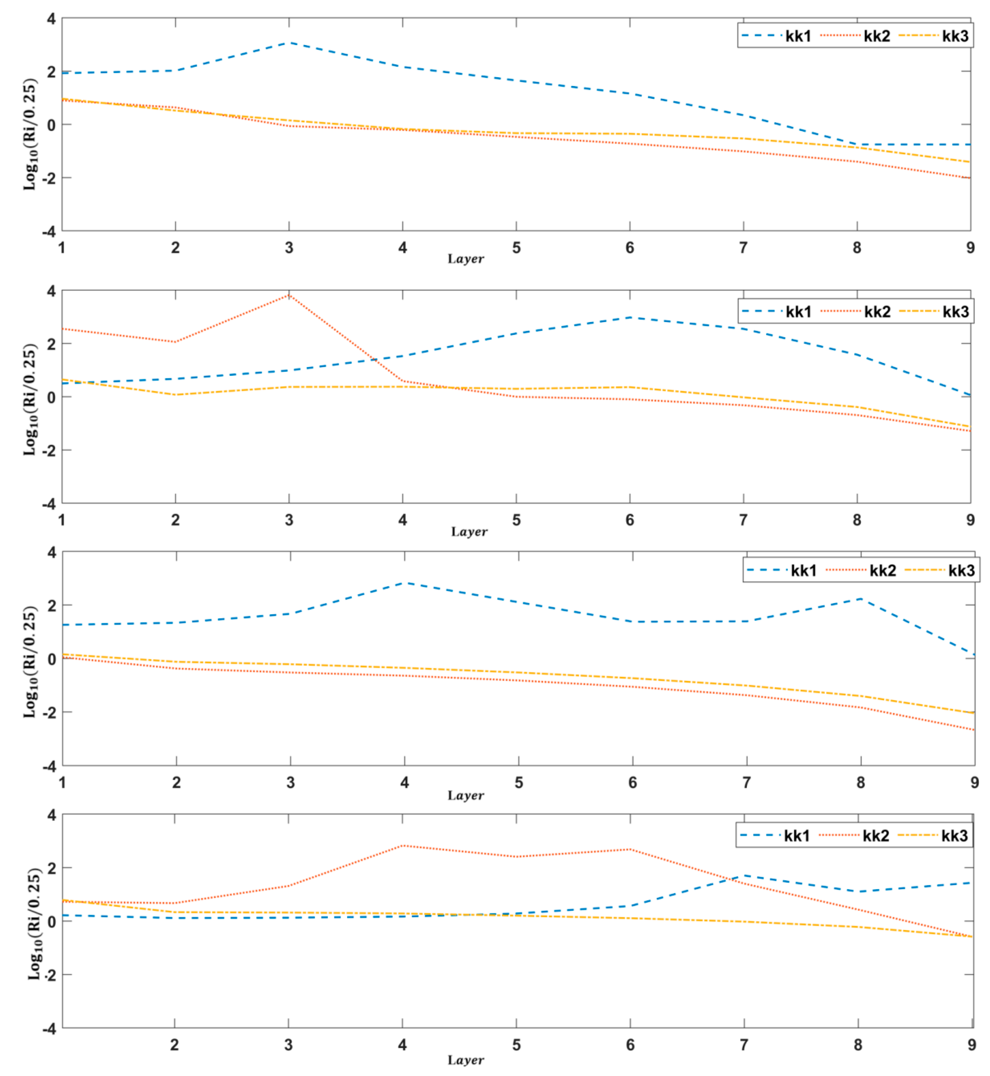
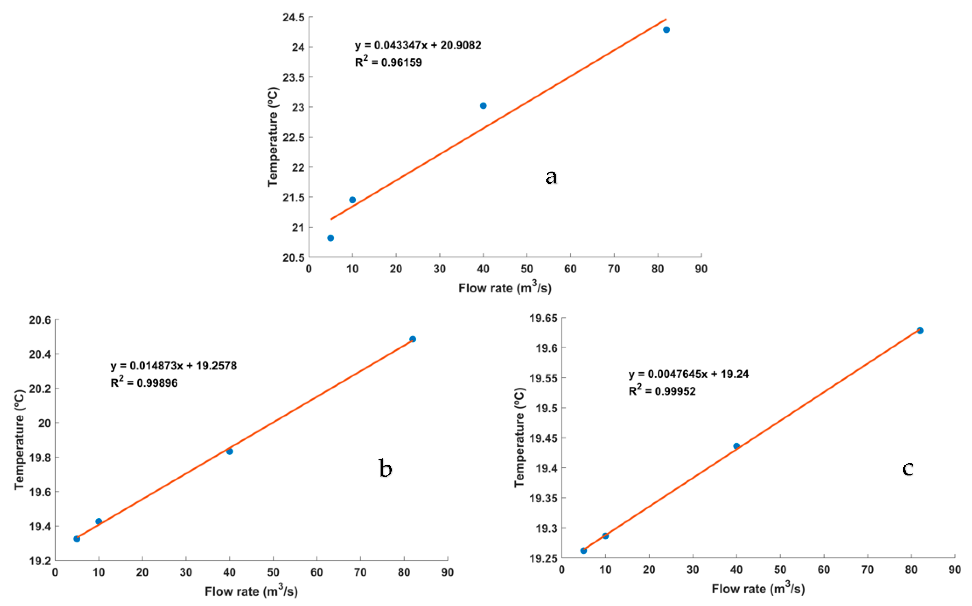
4.2.2. Analysis of Thermal Plume Mechanism

The diffusion characteristics of thermal plumes under different influencing factors have been analyzed. In this section, based on the changes in momentum, the mechanisms of how the discharge flow rate affects the thermal plume are investigated. Taking Wushashan Power Plant as an example, the momentum per unit volume at characteristic moments is calculated under different flow rate conditions.

$$Pv=\rho ·(U,V)$$

(13)

Here, $Pv$ represents the momentum per unit volume, ρ represents the seawater density taking into account the thermal discharge, while U and V denote the flow velocities.

Figure 7 presents the distribution of momentum per unit volume at the surface during the moments of flood rapid, flood slack, ebb rapid, and ebb slack. The momentum field is noticeably influenced by the tidal fluctuations, with only slight differences in momentum direction at the discharge outlet between the two flow rates, but showing a consistent pattern overall. With increasing flow rates, significant regions of increased momentum appear at all tidal phases, varying with the ebb and flood cycles. Moreover, considering the spreading of the thermal plume, it is observed that the direction of the increased momentum zone aligns with the direction of plume diffusion. Doubling the discharge flow rate leads to a substantial increase in momentum, consequently resulting in an expanded range of plume spreading.

4.3. Dispersion Characteristics and Mechanisms of Thermal Plume during Typhoon

4.3.1. Analysis of Thermal Plume Characteristics

By comparing and analyzing the spreading ranges of the thermal plume under three different scenarios (Figure 8 and Figure 9), it is found that the surface thermal plume is significantly influenced by the intensity and path of typhoons. Under Exp8, the thermal plume spreads almost perpendicular to the coastline, with a slight deviation towards the mouth of the estuary, which is attributed to the relatively lower flow velocity during the peak of the storm surge. When the intensity of the typhoon is halved, the spreading range of the thermal plume noticeably increases and expands towards the mouth of the estuary. With a change in the typhoon’s path, the spreading direction of the thermal plume also changes, shifting from the direction of the estuary to the direction of the bay’s top, and the spreading becomes closer to the coastline. On the other hand, the bottom layer is less affected by the intensity and path of typhoons, resulting in a relatively smaller spreading range.

A cross-section near the power plant was selected (Figure 5a), and the vertical temperature distribution along the cross-section during the peak storm surge was calculated and analyzed (Figure 10). When the intensity of the typhoon is halved, the spreading range of the thermal plume increases. Considering the horizontal distribution and the position of the cross-section, the weakening effect of the wind field on the flow field is minimal when the intensity is halved, and the flow velocity near the power plant is relatively high. As a result, the spreading range is larger in the direction perpendicular to the power plant. Therefore, the impact is significant along the direction of the cross-section. When the typhoon path changes, the spreading range of the surface thermal plume is relatively smaller. Considering the horizontal spreading of the thermal plume and the distribution of the flow field, during the path change, the direction and magnitude of the wind speed near the power plant change, not only weakening the inherent flow field in the surface layer but also causing flow reversal. Consequently, the spreading direction of the thermal discharge plume deviates more towards the top of the bay and becomes closer to the southern coast. As a result, the spreading range along the cross-section is relatively smaller.

In order to study the mixing characteristics near the power plant, the Richardson numbers at different working conditions and feature points are calculated respectively (Figure 11). At the kk1 point, under Exp9, the maximum value of log₁₀(Ri/0.25) is observed at the surface. Combining it with the distribution of the surface thermal plume, it is evident that the kk1 point is most affected by the thermal discharge in Exp9, and log₁₀(Ri/0.25) decreases with increasing depth. Under Exp10, log₁₀(Ri/0.25) shows minimal variation with depth. In Exp8, log₁₀(Ri/0.25) increases from the surface to a certain depth and then decreases. This trend is attributed to the surface being located in the high-temperature region, transitioning to the transitional zone, and finally entering the low-temperature region. The transitional zone exhibits the maximum value of log₁₀(Ri/0.25).

At the kk2 point, the surface still has the highest value of log₁₀(Ri/0.25) in Exp9. Considering the thermal plume distribution, it is evident that the surface is most influenced by the thermal discharge at this point. The log₁₀(Ri/0.25) value continues to increase until reaching the thermal transition zone before decreasing. In Exp8, a similar trend of increasing (reaching the transition zone) and then decreasing is observed. In Exp10, log₁₀(Ri/0.25) initially increases until reaching the transition zone before decreasing. Subsequently, it increases again and then decreases.

At the kk3 point, all three scenarios exhibit an initial increase followed by a decrease in log₁₀(Ri/0.25). In Exp9, it increases to its maximum value first, followed by Exp8, and finally, Exp10c reaches its maximum value. In terms of flow velocity, the surface velocity is the smallest in Exp9 and gradually decreases from top to bottom. It reaches the transition zone first. Exp8 has a slightly higher velocity, and Exp10 has the highest velocity. The surface and bottom velocities exhibit a reverse trend, with the bottom velocity reaching the transition zone last.

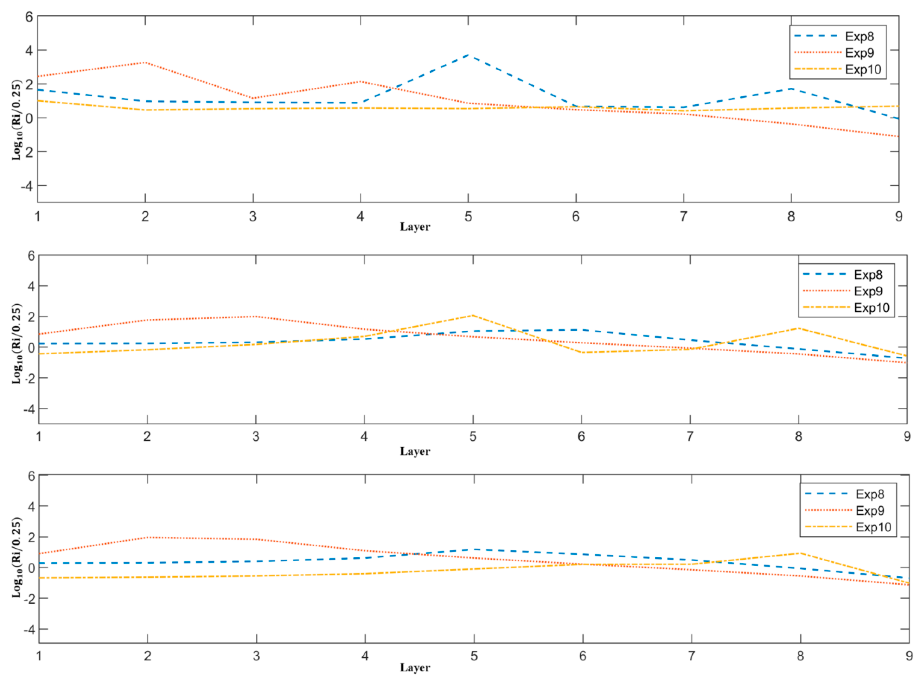
4.3.2. Analysis of Thermal Plume Mechanism

To investigate the diffusion mechanism of the surface temperature rise plume, we conducted calculations and analyses of the wind field (Figure 12) and flow field characteristics (Figure 13) in the vicinity of the power plant at corresponding times. The flow field direction is opposite to the wind speed direction, with the wind field exerting a weakening effect on the surface flow field. Halving the intensity of the typhoon reduces the wind speed by half, diminishing the wind field’s weakening effect on the surface flow field. Consequently, the surface flow field expands, leading to an increased diffusion range of the temperature rise plume. The bottom flow field experiences minimal influence from the wind field, resulting in little change to the plume. When the typhoon track shifts, moving northward near Xiangshan Bay, the wind speeds increase in the area, and the wind direction shifts further southwestward. This alteration in the wind field affects the surface flow field, causing a shift in flow direction from northeast to southwest, consequently altering the diffusion direction of the temperature rise plume to the southwest. The bottom flow field, less impacted by surface wind patterns, maintains its original direction.

5. Discussion

Figure 14 demonstrates the spreading range of the thermal plume in different working conditions. Near the power plant, the spreading range of the surface thermal plume noticeably decreases as the flow rate decreases. Under normal flow conditions, the flow velocity of thermal discharge is less affected by the inherent flow velocity in the bay, and more conducive to spreading towards the center of the bay. However, when the flow rate is halved, the flow rate of thermal discharge is small, and the flow is greatly affected by the inherent flow in the bay (along the bay), so thermal discharge spreads along the bay. Comparing the surface layer areas enclosed by the 3 °C thermal anomaly contours before and after the flow rate change (

Table 2. Diffusion range of temperature rise plume.

	Spreading Area (Unit: ×103 m2)
	Peak Flood	High Slack Water	Peak Ebb	Low Slack Water
Exp1–Exp7	200.26	1005.67	261.13	602.81
Exp2–Exp7	95.76	208.72	78.58	175.58
Exp3–Exp7	199.98	1006.87	261.11	603.80
Exp4–Exp7	120.94	621.43	311.44	632.08
Exp5–Exp7	10.79	31.65	12.63	31.74
Exp6–Exp7	4.06	13.67	3.96	13.24

), it is observed that a significant reduction in the thermal anomaly contour areas near the power plant occurs at all tidal phases when the flow rate is halved.

Figure 14 illustrates the spreading characteristics of the thermal plume without considering the Coriolis force effect. Comparing the results with and without considering the Coriolis force, it can be observed that there is no significant variation in the spreading of the surface thermal plume near the power plant in both cases. This indicates that the Coriolis force has little influence on the diffusion of the thermal discharge, as there are no apparent changes observed during the high slack water, peak flood, low slack water, or peak ebb.

Through comparing the spreading characteristics of the surface discharge case and the bottom discharge case of the thermal plume, the impact of the discharge method on the spreading of the thermal plume is analyzed. The comparative analysis of the thermal plume spreading range reveals an overall reduction in the spreading range. Among the tidal phases, the high slack water moment shows the largest decrease in spreading range, with a decrease of 384.24 × 10³ m² in the area enclosed by the 3 °C thermal anomaly contour. The peak flood moment exhibits the second highest reduction with a decrease of 79.32 × 10³ m² in the spreading area. On the other hand, the low slack water and peak ebb moments show a slight increase in the spreading area (Table 2).

Numerical experiments (Exp5, Exp6) were designed to investigate the critical discharge flow rate for the generation of thermal plumes and the size of the resulting plumes (Table 1). Exp5 and Exp6 obtained the temperature fields considering the influence of thermal discharge. By subtracting the temperature field obtained from Exp7, which did not consider the thermal discharge, the thermal anomaly fields for both cases were derived. The spreading of a 3 °C thermal plume was calculated, and the corresponding spreading areas were determined (Table 2). A comparative analysis of the results revealed a significant reduction in the spreading area of the thermal plume when the flow rate was lower (5 m³/s). Specifically, the spreading area of the 3 °C thermal plume at a flow rate of 5 m³/s was less than 1/40 of the normal condition. This indicates that the influence of thermal discharge on the nearby seawater temperature is relatively small under such conditions.

To examine the influence of discharge flow rate on water temperature at three selected characteristic points (kk1, kk2, kk3) near the power plant (Figure 5), the average temperature values over 14 tidal cycles (174 h) were calculated. Based on experimental data from Exp1, Exp2, Exp5, and Exp6, linear regression analysis was performed to establish the regression equations between the temperature at the characteristic points and the thermal discharge flow rate. The regression curves and corresponding fitting formulas are presented in Figure 15, providing insights into the relationship between flow rate and seawater temperature.

Figure 15 reveals that the seawater temperature increases with the increase in flow rate. There is a strong positive correlation between flow rate and seawater temperature, with correlation coefficients consistently above 0.9. Moreover, it can be observed that the closer the characteristic point is to the power plant, the steeper the slope of the fitting function (kk1 > kk2 > kk3). This indicates that the temperature is more sensitive to variations in flow rate near the power plant. Additionally, at the same flow rate, the temperature is higher when the point is located closer to the power plant, indicating a greater impact of the power plant on the temperature.

6. Conclusions

This study, based on the FVCOM ocean numerical model, investigates the characteristics and variations of temperature-rise plume generated by Wushashan Power Plant in Xiangshan Bay. This study focuses on understanding the different variations in the plume flow under normal weather conditions and typhoon weather conditions. Based on the optimized numerical model and combined with mathematical statistical methods, the diffusion range of the thermal plume by thermal discharge was studied, and the diffusion characteristics and mechanisms were explored. The flow rate affects the plume flow through the momentum at the discharge outlet, and the temperature rise plume flow exhibits evident stratification phenomena under normal weather conditions. During a typhoon, the intensity and path of the typhoon influence the diffusion range of the thermal plume, with a greater impact on the surface layer. The wind field primarily affects the diffusion of the plume flow through its influence on the surface flow field.

This study primarily relies on numerical simulations. Integrating laboratory physical models to investigate local thermal discharge diffusion patterns would enhance the depth of our research. Future endeavors will involve constructing physical models to delve deeper into the diffusion mechanisms of thermal discharge. Furthermore, while this study focuses on power plants situated in semi-enclosed bays, variations may exist for those in open-sea environments. Subsequent investigations will explore the thermal discharge diffusion dynamics of open-sea power plants, comparing them with those in semi-enclosed bays to broaden the scope of our findings.

References

1. Miao, Q.; Zhou, L.M.; Deng, Z.Q. Measurement and numerical simulation of thermal discharge from Xiangshan Port power plant. Coast. Eng. 2010, 29, 1–11. [Google Scholar]
2. Zhang, C.L.; Liang, C.L.; Zhang, J.Y.; Shi, H.G. Remote sensing monitoring of thermal discharge from Tianwan Nuclear Power Station based on Landsat-8 TIRS data. Geospat. Inf. 2019, 17, 70–72, 87. [Google Scholar] [CrossRef]
3. Zhang, W.Q.; Zhou, R.M. Thermal impact analysis of Daya Bay Nuclear Power Station and Ling’ao Nuclear Power Station effluent discharge. Radiat. Prot. 2004, 24, 257–262. [Google Scholar]
4. Wang, G.L.; Xiong, X.J. Analysis of thermal discharge distribution and variations in the Tianwan Sea area. Adv. Mar. Sci. 2013, 31, 69–74. [Google Scholar]
5. Zhao, Q.; Cao, W.; Xing, J.; Long, S.Q. Analysis of spatial and temporal characteristics of winter thermal discharge in Sanmen Nuclear Power Plant based on field observation data. Mar. Environ. Sci. 2022, 41, 847–856. [Google Scholar] [CrossRef]
6. Bush, R.M.; Welch, E.B.; Mar, B.W. Potential effects of thermal discharges on aquatic systems. Environ. Sci. Technol. 1974, 8, 561–568. [Google Scholar] [CrossRef]
7. Jiang, W.; Lin, Y.J.; Lu, Y.H. Experimental research method and application of cooling water project in tidal river channels. J. Guangzhou Univ. (Nat. Sci. Ed.) 2001, 15, 43–47. [Google Scholar]
8. Yang, H.Y. Experimental study on thermal discharge influenced by tidal flow. Guizhou Water Power 2005, 19, 75–78. [Google Scholar]
9. Wang, Y.; Luo, A.; Lu, H.Z. Physical model test on thermal discharge of new construction project of Lufeng Jiahuwan Power Plant. Guangdong Water Conserv. Hydropower 2015, 1–5. [Google Scholar]
10. Liang, H.H.; Kang, Z.S. Physical model test of thermal discharge in the second phase of Hongyanhe nuclear power plant. In Proceedings of the Thesis of the 6th National Conference on Hydraulics and Water Informatics, Beijing, China, 8 June 2013; pp. 82–88. [Google Scholar]
11. Tang, D.L.; Kester, D.R.; Wang, Z.d.; Lian, J.S.; Kawamura, H. AVHRR satellite remote sensing and shipboard measurements of the thermal plume from the Daya Bay nuclear power station, China. Remote Sens. Environ. 2003, 84, 506–515. [Google Scholar] [CrossRef]
12. Qin, Z.H.; Li, W.J.; Zhang, M.H.; Arnon, K.; Pedro, B. Estimation method of atmospheric parameters based on single-window algorithm. Remote Sens. Land Resour. 2003, 37–43. [Google Scholar] [CrossRef]
13. Xu, H.P.; Ma, Y.; Zhao, X.S. Application research of Landsat-8 satellite imagery in thermal discharge monitoring of nuclear power plants. In Proceedings of the 6th Annual Conference of the China Risk Assessment Committee on Information Technology in Risk Analysis and Crisis Response, Hohhot, Inner Mongolia, China, 23 August 2014; pp. 836–839. [Google Scholar]
14. Gu, H.Q.; Zou, G.L.; Ma, J.R. Application of Landsat-8 TIRS data in thermal discharge monitoring of a nuclear power plant. Mar. Sci. 2016, 40, 76–81. [Google Scholar]
15. Xu, J.; Zhu, L.; Jiang, J.; Li, J.G.; Zhao, S.H.; Yuan, L. Remote sensing monitoring of thermal discharge from Daya Bay Nuclear Power Base based on HJ-1B and TM thermal infrared data. Environ. Sci. China 2014, 34, 1181–1186. [Google Scholar]
16. Yang, H.Y.; Zhu, L.; Wu, C.Q.; Jia, X.; Zhao, H. Remote sensing monitoring and environmental impact analysis of thermal discharge from nuclear power plants. Environ. Prot. 2018, 46, 18–22. [Google Scholar] [CrossRef]
17. Huang, X.Q.; Ye, S.F. Monitoring and Impact Assessment of Thermal Discharge from Xiangshan Port Power Plant; Ocean Press: North Melbourne, VIC, Australia, 2014. [Google Scholar]
18. Xia, Y.Y.; Liu, Z.M.; Cui, Y.S.; Mou, W.T.; Lv, H.B. Spatiotemporal characteristics of thermal discharge from Sheyang Port power plant based on Landsat data. J. Jiangsu Ocean Univ. (Nat. Sci. Ed.) 2022, 31, 42–48. [Google Scholar]
19. Lin, J.; Zhang, S.Y.; Gong, F.X. Numerical simulation study on site selection evaluation of marine ranching planning area of Xiangshan Port: Influence of thermal discharge from coastal power plants. J. Shanghai Ocean Univ. 2012, 21, 816–824. [Google Scholar]
20. Chen, Z.J.; Zeng, Z.; Chen, C.H.; Tang, J.J. Study on plane distribution and vertical variation of temperature rise under the influence of thermal discharge from coastal power plants: A case study of Kemen Power Plant in Luoyuan Bay. Mar. Environ. Sci. 2023, 42, 111–121. [Google Scholar]
21. Chen, H. Research on Mathematical Models of Thermal Discharge from Houshi Power Plant; Xiamen University: Xiamen, China, 2002. [Google Scholar]
22. Liu, H.C.; Chen, H.B. Application of unstructured grid in the numerical model of thermal discharge from Yacheng Power Plant in Indonesia. Waterw. Port 2009, 30, 316–319. [Google Scholar]
23. Sun, X.M.; Zhang, L.G. Prediction method and application of thermal pollution in thermal power plants. Environ. Prot. Circ. Econ. 2001, 21, 30–31. [Google Scholar]
24. Zhang, J.M.; Wu, S.Q.; Wang, H.M. Analysis of flow characteristics and research on model parameters in thermal discharge areas of power plants. Northeast Water Conserv. Hydropower 2005, 23, 51–52. [Google Scholar]
25. Duan, Y.F.; Zhao, Y.J.; Ji, P.; Zhang, B.B. Comparison between water tank test and numerical simulation of thermal discharge and the distribution of water temperature. J. Hydroelectr. Eng. 2017, 36, 100–110. [Google Scholar]
26. Yanagi, T.; Sugimatsu, K.; Shibaki, H.; Shin, H.; Kim, H. Effect of tidal flat on the thermal effluent dispersion from a power plant. J. Geophys. Res. 2005, 110, 1–15. [Google Scholar] [CrossRef]
27. Zhang, G.J. Study on Three-Dimensional Numerical Simulation of Thermal Discharge in the Northern Longkou Sea Area; First Institute of Oceanography, State Oceanic Administration: Qingdao, China, 2015. [Google Scholar] [CrossRef]
28. Gu, J.; Han, X.J.; Kuang, C.P.; Zhang, J.Y.; Zuo, L.L.; Zhu, Q. Three-dimensional simulation and analysis of thermal discharge transport in estuaries, lagoons, and coastal areas. J. Hydrodyn. Ser. A 2020, 35, 201–212. [Google Scholar]
29. You, Z.J.; Jiao, H.F. Ecological Environment Protection and Restoration Techniques in Xiangshan Port; Ocean Press: London, UK, 2011. [Google Scholar]
30. Chen, C.S.; Beardsley, R.C.; Cowles, G. An Unstructured Grid, Finite-Volume Coastal Ocean Model: FVCOM User Manual; Smast/Umassd: Boston, MA, USA, 2006. [Google Scholar]
31. Pawlowicz, R.; Beardsley, B.; Lentz, S. Classical tidal harmonic analysis including error estimates in MATLAB using T_TIDE. Comput. Geosci. 2002, 28, 929–937. [Google Scholar] [CrossRef]
32. Ye, T.Y. Multi-Temporal and Spatial Scale Dynamics of Suspended Sediment in Hangzhou Bay and the Feedback Mechanism with Tidal Flat Changes; Zhejiang University: Hangzhou, China, 2019. [Google Scholar]
33. Kong, G.Q.; Li, L.; Guan, W.B. Influences of tidal flat and thermal discharge on heat dynamics in Xiangshan Bay. Front. Mar. Sci. 2022, 9, 1–17. [Google Scholar] [CrossRef]
34. Monismith, S.G. Contemporary Issues in Estuarine Physics: Mixing in Estuaries; Cambridge University: Cambridge, UK, 2010; pp. 145–185. [Google Scholar]
35. Geyer, W.R.; Maccready, P. The estuarine circulation. Annu. Rev. Fluid Mech. 2014, 46, 299–305. [Google Scholar] [CrossRef]
36. Bigg, P.H. Density of water in SI units over the range 0–40 °C. Br. J. Appl. Phys. 2002, 18, 521–525. [Google Scholar] [CrossRef]
37. Yao, Y.M.; Zheng, Y.Q.; Zhao, X.Y.; Yuan, J.X.; Li, L. Characteristics of stratification in the Jiaojiang Estuary. Haiyang Xuebao 2021, 43, 23–37. [Google Scholar]
38. Miles, J.W. On the stability of heterogeneous shear flows. J. Fluid Mech. 1961, 10, 496–508. [Google Scholar] [CrossRef]
39. Fu, D.T.; Xie, C.C.; Wu, J.B.; Wei, Y.L. Water stability and its influencing factors in the adjacent waters of the Yangtze River Estuary. J. Xiamen Univ. (Nat. Sci. Ed.) 2020, 59, 39–45. [Google Scholar] [CrossRef]
Figure 1. (a) Geographical location of Xiangshan Bay (https://earth.google.com/); (b) grid within Xiangshan Bay; (c) grid near the power plant; (d) diagram of thermal discharge outlet.
Jmse 12 00429 g001
Figure 2. Distribution of flow field of surface layer near Wushashan Power Plant ((a) peak flood, (b) high slack water, (c) peak ebb, (d) low slack water).
Jmse 12 00429 g002
Figure 3. Distribution of flow field of bottom layer near Wushashan Power Plant ((a) peak flood, (b) high slack water, (c) peak ebb, (d) low slack water).
Jmse 12 00429 g003
Figure 4. Diffusion range of temperature rise plume under Exp1 ((a) peak flood, (b) high slack water, (c) peak ebb, (d) low slack water). (The number represents the temperature rise in the picture).
Jmse 12 00429 g004
Figure 5. (a) Cross-section and location of characteristic points near Wushashan Power Plant; (be) vertical distribution of temperature field at the cross-section ((b) peak flood, (c) high slack water, (d) peak ebb, (e) low slack water).
Jmse 12 00429 g005
Figure 6. Variation in log10(Ri/0.25) values with depth (from top to bottom: peak flood, high slack water, peak ebb, low slack water).
Jmse 12 00429 g006
Figure 7. The momentum change near Wushashan Power Plant before and after the flow change (the background color represents the difference between Exp1 and Exp2, the red arrow represents Exp1, and the black arrow represents Exp2; (a) peak flood, (b) high slack water, (c) peak ebb, (d) low slack water).
Jmse 12 00429 g007
Figure 8. Distribution of surface temperature rise plume near Wushashan Power Plant. ((a) Exp8–Exp11; (b) Exp9–Exp 12; (c) Exp10–Exp 13).
Jmse 12 00429 g008
Figure 9. Distribution of bottom temperature rise plume near Wushashan Power Plant. ((a) Exp8–Exp11; (b) Exp9–Exp 12; (c) Exp10–Exp 13).
Jmse 12 00429 g009
Figure 10. Vertical temperature distribution near the power plant. ((a) Exp8–Exp11; (b) Exp9–Exp 12; (c) Exp10–Exp 13).
Jmse 12 00429 g010
Figure 11. The value of log10(Ri/0.25) varies with depth. (From top to bottom: kk1, kk2, kk3).
Jmse 12 00429 g011
Figure 12. The wind field near Wushashan Power Plant (the arrow indicates the direction of the wind field, and the color indicates the surface temperature rise; (a) Exp8–Exp11, (b) Exp9–Exp 12, (c) Exp10–Exp 13).
Jmse 12 00429 g012
Figure 13. The surface flow field near Wushashan Power Plant (arrow represents the direction of the flow field, color represents the flow rate; (a,c,e) surface, (b,d,f) bottom layer; (a,b) Exp8, (c,d) Exp9, (e,f) Exp10).
Jmse 12 00429 g013
Figure 14. The diffusion of temperature rise plume under different working conditions ((a,e,i) peak flood, (b,f,j) high slack water, (c,g,k) peak ebb, (d,h,l) low slack water; (ad) Exp2–Exp7; (eh) Exp3–Exp7; (il) Exp4–Exp7).
Jmse 12 00429 g014
Figure 15. Correlation analysis between discharge flow rate and temperature ((a) kk1 point; (b) kk2 point; (c) kk3 point).
Jmse 12 00429 g015