Abstract
Ocean-water temperature and salinity are two vital properties that are required for weather-, climate-, and marine biology-related research. These properties are usually measured using disposable instruments at sparse locations, typically from tens to hundreds of kilometers apart. Laterally interpolating these sparse measurements provides smooth temperature and salinity distributions within the oceans, although they may not be very accurate. Marine seismic data, on the other hand, show visible reflections within the water-column which are primarily controlled by subtle sound-speed variations. Because these variations are functions of the temperature, salinity, and pressure, estimating sound-speed from marine seismic data and relating them to temperature and salinity have been attempted in the past. These seismically derived properties are of much higher lateral resolution (less than 25 m) than the sparse measurements and can be potentially used for climate and marine biology research. Estimating sound-speeds from seismic data, however, requires running iterative seismic inversions, which need a good initial model. Currently practiced ways to generate this initial model are computationally challenging, labor-intensive, and subject to human error and bias. In this research, we outline an automated method to generate the initial model which is neither computational and labor-intensive nor prone to human errors and biases. We also use a two-step process of, first, estimating the sound-speed from seismic inversion data and then estimating the salinity and temperature. Furthermore, by applying this method to real seismic data, we demonstrate the feasibility of our approach and discuss how the use of machine learning can further improve the computational efficiency of the method and make an impact on the future of climate modeling, weather prediction, and marine biology research.
1. Introduction
Oceanic temperature and salinity distributions are major drivers of ocean dynamics such as meridional overturning circulation and oceanic turbulence [1]. These salinity and temperature distributions within the world’s oceans, in conjunction with atmosphere–hydrosphere interactions, have been related to the recent climatic variations [2,3] and have been used in developing models for predicting the frequency, intensity, and severity of future hurricanes [4]. Additionally, the variations in temperature and salinity due to global climate change and their effects in aquatic lives and controlling the production and migration of fish in marine, lake, and river environments have been thoroughly studied [5,6,7,8]. Thus, accurately estimating the temperature and salinity distributions within oceans, lakes, and rivers is important for global climate change research in a wide variety of disciplines such as physical oceanography, atmospheric science, marine biology, and the fishery industry.
The primary problem in using temperature and salinity is the accuracy of their measurements [9]. Oceanic temperature and salinity are measured using eXpendable BathyThermograph (XBT) and conductivity-temperature-depth (CTD) sensors, which can provide a regional temperature–salinity (T-S) relationship [10]. These estimates have a high vertical resolution (~1 m). In general, however, these XBT or CTD sensors are sparsely deployed, and thus, their lateral resolutions can be low [11]. These vertically high-resolution measurements at sparse lateral locations, when interpolated, may not have high lateral resolutions [11].
Temperature and salinity variations within water-column structures produce visible reflections on the recorded seismic data, which, in turn, allows for imaging of structures like ocean fronts, mesoscale eddies, and Lee waves [12,13,14,15,16]. In addition, dynamic processes such as ocean turbulence [17,18,19] and the movement of water masses [20,21] have also been recorded from these reflections. These techniques are sensitive to oceanic sound-speed variations [22] and can be applied to both two- and three-dimensional (2D and 3D) offshore seismic data [23].
Besides analyzing seismic images, extracting the thermohaline nature of oceans from seismic reflections has been attempted by many, which resulted in the emergence of a new field known as Seismic Oceanography. For example, it has been verified that the temperature contrasts in ocean waters can explain the amplitude-variation-with-angle (AVA) behavior of water-column seismic reflections [24]. Extracting accurate velocities (sound-speeds) using post-stack, pre-stack, and stochastic inversion methods to estimate temperature and salinity have also been attempted [25,26,27,28,29,30,31,32,33,34,35,36,37,38,39,40]. Most of these inversions allow for extraction of the high-frequency sound-speed variations within water-columns but require the low-frequency (background) trends to be available from other sources such as XBTs or CTDs. Because it is impossible to deploy many XBTs or CTDs, accurately estimating the background sound-speed variations is difficult. Therefore, estimating the broad-band sound-speed structures of the world’s oceans and relating them to the temperature and salinity using these methods is not an easy task. The main issue with these inversions is that most of these methods use a linearized (gradient-based) local optimization. Padhi et al. (2015) [11] demonstrated that, when a good background model is available, these local methods work very well. However, using a global optimization method, such as a genetic algorithm (GA), can obtain reliable sound-speed models even when such background trends are unavailable. Additionally, Padhi et al. (2015) [11] also showed how these estimated sound-speeds can be combined with the equation of state [41,42,43,44] and make reliable temperature and salinity profiles. These seismically derived temperature and salinity estimates are of lower vertical resolution (~5 m) than those obtainable from XBT or CDT data. However, they are of high lateral resolution (25 m or less) [11], which can potentially open entirely new avenues for physical oceanography, climate, marine biology, and fishery research.
Although the sound-speed can be accurately estimated from marine seismic data, using which the temperature and salinity can also be estimated, it is difficult to use them on a routine basis. Reasons for this have been thoroughly studied elsewhere [45]. For completeness, we briefly discuss these reasons and introduce the motivation of our current research.
Figure 1 summarizes one of the current practices of estimating the sound-speed from the pre-stack seismic data [11]. Because of their inherent non-uniqueness and computationally demanding nature [46], seismic inversions require an initial model. The primary reason for this requirement is to ensure that the inversion finds a meaningful, not an undesired, solution. For sound-speed estimation, if XBT and CTD data coincide with the seismic data, then an initial sound-speed can be estimated using the equation of state [41,42,43]. However, XBT/CTD may be available only at sparse locations or may not be available at all. To resolve this issue, Padhi et al. (2015) [11] ran pre-stack GA inversion [47,48,49] at a few sparse locations and estimated the sound-speed for those locations. In the real stacked seismic data from the South China Sea, shown in Figure 1a, these locations are indicated by arrows. After estimating sound-speeds at sparse locations, their low-frequency estimates were interpolated along three horizons, which Padhi et al. (2015) [11] manually interpreted from the stacked seismic data. These interpreted horizons are shown as green lines in Figure 1a and the sound-speed model from interpolation is shown in Figure 1b. Using this interpolated model as the initial model for each common midpoint (CMP) location, Padhi et al. (2015) [11] ran prestack waveform inversion using both the GA and nonlinear least square (NLS) methods and estimated the sound-speed for the entire range of the data, and Figure 1c is the GA inversion result.
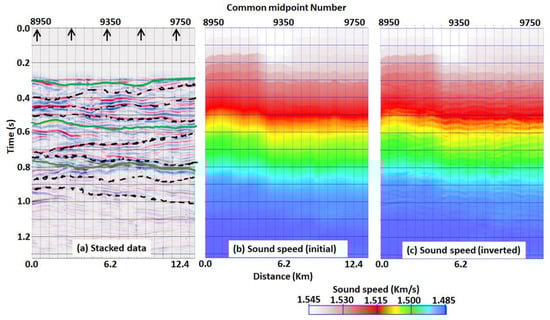
Figure 1.
The currently accepted process for sound-speed estimation from pre-stack seismic data. (a) Stacked seismic data from South China Sea showing reflections within the water-column. The arrows on top indicate five sparse locations where separate inversions were first run as a process to generate the initial model. Three green lines are three separate horizons which were manually interpreted from the stacked data and the dashed black curves are additional horizons, the picking of which can modify both initial and inverted models. (b) Initial sound-speed model. The low-frequency sound-speeds from the inversion at the five sparse locations were laterally interpolated along the three green horizons to generate this model. (c) Final sound-speed model estimated from inversion. This figure is modified from Mallick and Chakraborty (2022) [45].
Horizon-guided interpolation for initial model generation (Figure 1b) is a standard practice in seismic inversion. For inversion to produce meaningful results, such an interpolation is considered necessary [21,50]. However, if we compare Figure 1b,c, it is obvious that such horizon-guided interpolation tends to bias the inverted model by leaving the imprint of the originally picked horizons in the final model. If additional horizons are picked, for example, the ones shown as dashed black lines in Figure 1a, then the initial model and the final model will be different from those shown in Figure 1b,c. Not only does this bias depend upon the number of horizons, but it is also likely to vary from person to person, based on the way they are being picked from the stacked seismic data. In addition, although many sophisticated automated horizon interpretation procedures are available, including the machine learning-based methods, none of them are error-free and any picking error is likely to be propagated in the inverted sound-speed.
In Figure 1, we show a 2D case where horizon-picking is straightforward. For 3D seismic data, manually picking horizons for the entire data volume is impossible. Therefore, the horizons are picked at regular inline or crossline intervals and then spatially interpolated to obtain horizon surfaces [51]. This spatial interpolation is not error-free and any error is likely to be propagated in the inversion results. Consequently, finding a way to obtain a bias-free (and error-free) inversion where no horizon picking is necessary is desirable [52].
Besides horizon-guided initial model generation, running GA inversion at sparse locations is computationally challenging. To generate a consistent model for the entire data range, these inversions must be carefully run, which involves a lot of expertise and human labor. In the example shown in Figure 1, these sparse inversions were run only at five locations. For large 3D data volumes, a lot more such inversions involving additional human labor and computation time would be necessary, the avoidance of which is desirable.
Irrespective of the method used for seismic inversion, the goal of seismic oceanography is to map the inverted sound-speeds onto the temperature and salinity. To simultaneously estimate the temperature (T) and salinity (S) from the inverted sound-speeds (V) requires calculating pressure as a function of depth and latitude [44]. Then, starting with an initial salinity model, it must be iteratively modified using an inversion (optimization) until it is reasonably matched with the regional T-S relationship of the CTD data from the Levitus database [10]. This step is also another computationally challenging task and requires a regional T-S relationship, which may not always be available. Therefore, it is preferable that we find an alternate, automated V to T-S mapping methodology.
For estimating the sound-speed, a data-driven, attribute-guided method to generate the initial model has been recently developed, which does not require any separate inversions at sparse locations or horizon interpretation [45]. This method is therefore neither subject to the human errors and biases involved in horizon-picking, nor it is subject to the additional computational expense and human labor caused by sparse inversion runs [45]. In this work, we outline a two-step approach for estimating and from seismic data. In the first step, we estimate using the data-driven, attribute-guided inversion of the marine seismic data [45]. In step 2, we develop an inversion method using the Adaptive Moment (ADAM) optimization [53] and use it to estimate and from .
In the following, we first outline our two-step approach along with the results from the South China Sea seismic data. Next, we discuss results and the possibilities for future improvements by converting our two-step approach into a single step using machine learning. Finally, we end with some concluding remarks.
2. Methodology and Results
Our two-step approach consists of (1) data-driven and attribute-guided inversion of seismic data for estimating the sound-speed and (2) estimation of the temperature and salinity from the inverted sound-speed from step 1. Below, we separately discuss each of them.
Step-1, data-driven, attribute-guided inversion for sound-speed estimation: Details of the data-driven and attribute-guided inversion can be found elsewhere [45]. Here, we briefly summarize the fundamental steps along with the results from the South China Sea marine seismic data.
The first step in the data-driven, attribute-guided approach is estimating the initial velocity (sound-speed). Instead of running sparse inversions, we perform velocity analysis (VELAN) at every 50th CMP location and then laterally interpolate them on a sample-by-sample basis, not guided via any interpreted horizons as an initial estimate of the sound-speed. Figure 2a is the sound-speed estimated from VELAN and interpolation. Comparing Figure 2a with the initial sound-speed model shown in Figure 1b, we can see that the general values in both are similar, with high values (white-to-red zone with 1.55–1.51 km/s sound-speed) for ~0–0.6 s, moderate values (yellow-green zone with 1.51–1.48 km/s sound-speed) for 0.6–1s, and low values (blue zone with sound-speed less than 1.48 km/s) below 1s. However, there is no apparent horizon-induced bias in the sound-speed shown in Figure 2a like that shown in Figure 1b. Following VELAN and lateral interpolation, we apply the geometrical spreading compensation (GSC) to the pre-stack gathers, correct them for the normal moveout (NMO), and stack them. Figure 2b shows the stacked data. Because VELAN, GSC, NMO, and stacking are standard and automated procedures in seismic data processing [54], this step is fully automated and not prone to any bias or errors due to horizon-picking. In addition, because no individual GA inversions at sparse locations are required, the process does not involve much computational expense or human labor, and is therefore applicable to 3D applications.
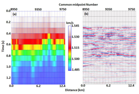
Figure 2.
(a) Sound-speed estimated from velocity analysis and lateral (sample-by-sample) interpolation. (b) Data after GSC, NMO correction and stacking.
Following stacking, we compute the time-domain attribute where is the time from the stacked seismic data as
In Equation (1), is the stacked seismic data and is computed from using the following steps:
- Forward Fourier transform to where is the frequency;
- Interchange the real and imaginary parts of and obtain . Thus, for any sample , if of is , then the corresponding sample of is , where ;
- Inverse Fourier transform and take its real part as .
Thus, the attribute is directly computable from the stacked data shown in Figure 2b.
Figure 3 is the attribute-guided approach to generate the initial model for inversion. Figure 3a is the cross-plot between the attribute on the horizontal axis and the VELAN and interpolation-estimated sound-speed on the vertical axis for the same five locations, indicated by arrows in Figure 1a, where GA inversions were run to generate the initial model of Figure 1b with the plotted points shown as black dots (circles). The red curve shown in this figure is the best-fit polynomial between the points, which gives the sound-speed as a function of , as
in which is in m/s. The value in the fit given by Equation (2) is 0.8741. Using Equation (2), we compute from for the entire range of the seismic data, and it is shown in Figure 3b. Like Figure 1b,c and Figure 2a, the attribute-guided sound-speed model shown in Figure 3b is also represented by the high (white to red), moderate (yellow to green) and low (blue) sound-speed zones at the similar time intervals.
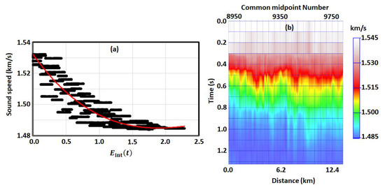
Figure 3.
The process of generating the attribute ()-guided initial model. (a) versus sound-speed () cross-plot for the same five locations marked by arrows in Figure 1a with the plotted points shown as black dots and the best-fit polynomial in red. (b) Sound-speed computed from using the equation represented by the red curve shown in (a).
Using the sound-speed shown in Figure 3b as the initial model, we run the GA-based pre-stack waveform inversion and show the inverted model in Figure 4 in both the time (Figure 4a) and depth (Figure 4b) domains. Notice that, although we did not provide any horizon information in the initial model, the inverted sound-speed model (Figure 4) is in perfect agreement with the reflection boundaries in the stacked seismic data (Figure 1a and Figure 2b), as if each of these reflection boundaries were separately picked as horizons and the initial model was guided through them. By computing wave equation-based pre-stack synthetic seismic data using the depth-domain model shown in Figure 4b and for the same range of source-to-receiver offsets as they were in real data, followed by GSC and NMO correction and stacking, it was further verified that the synthetic stacked data matched almost perfectly with the real stacked data, giving additional confidence in the reliability of the estimated sound-speed model shown in Figure 4 [45]. Although the inverted sound-speed model obtained earlier by the horizon-guided approach [11], shown in Figure 1, produced synthetic stacked data which also matched real stacked data with equal accuracy, we must note that the latter results are biased by the picked horizons while the attribute-guided results are not. We must also note here that both horizon- and attribute-guided inversions require an initial density model in addition to the sound-speed. Density is an important parameter in physical oceanography. However, the fundamental basis for our analysis is seismic inversion, or, to be specific, quantifying the variations in the seismic reflection amplitudes as a function of the angle-of-incidence. In an earlier work, Mallick and Chakraborty (2022) [45] carried out a detailed investigation on the sensitivity of these water-column reflection amplitudes to the variations in the sound-speed and density. Their analysis revealed that the relative variations in these amplitudes are primarily controlled by the sound-speed, with density providing a bulk shift to the amplitudes without affecting their relative values. Considering that all seismic inversion methods are based on quantifying the relative amplitude variations, not their absolute values, we thus conclude that the density cannot be accurately estimated from the seismic data. Therefore, within the observed range of the water-column density variations which is approximately 1030–1070 kg/m3 [11,45], we assumed a constant density of 1050 kg/m3 for both inversions shown in Figure 1 and Figure 4, and in all our subsequent analyses.
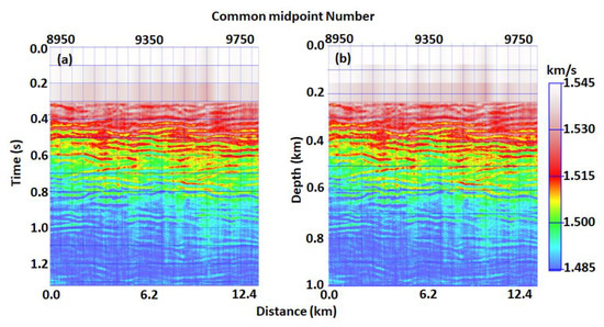
Figure 4.
Inverted sound-speed in (a) time and (b) depth domain using the attribute-guided model of Figure 3b as the initial model.
Step-2, simultaneous estimation of the temperature and salinity from the sound-speed: To estimate the temperature and salinity from the sound-speed, we first define our observed data as an -component sound-speed vector , given as
and the model to be estimated as -component model vector , given as
Clearly, in Equations (3) and (4) is the number of depth samples at each CMP location, with , , and being, respectively, the sound-speed, temperature, and salinity for the depth sample. Given the sound-speed vector from the seismic inversion for each CMP location (Equation (3)), our goal is to estimate the -component model vector (Equation (4)), in which the first -components are the temperatures and the next -components are the salinity for those CMP locations.
Estimating the -component model vector of the temperature and salinity from the observed -component data obtained from seismic inversion is an optimization problem. To solve this problem, we used the Adaptive Moment Estimation method (ADAM) [53]. The ADAM is an iterative optimization algorithm used to minimize the loss function during the training of neural networks and became popular in the use of deep learning for adjusting the learning rate for each parameter in a model [55]. Although primarily used in machine learning, the ADAM is well-suited for any problem where the data and model sizes are large and the objectives are non-stationary with sparse or noisy gradients [55]. Because our problem of mapping the seismic sound-speed onto temperature and salinity falls in the same category, we chose the ADAM for optimization.
In our implementation, we first define our forward problem that each of Equation (3) is related to the and of Equation (4) and pressure where via the equation of state, given as
Exact expressions for , , , and in Equation (5) can be found elsewhere [41,42,43]. For completeness, we also provide them below in Appendix A. Note that our forward problem not only requires the temperature () and salinity () but also the pressure () for each depth sample . To iteratively update the temperature () and salinity (), it is first necessary to discuss how to calculate the pressure () in Equation (5).
The pressure as a function of depth () and latitude () is given as
In Equation (6), is the mean atmospheric pressure at sea level (101,325 Pa or 1.01325 bars), is the acceleration due to gravity at latitude and depth in m/s2, and is the density of seawater in kg/m3. The exact value of in Equation (6) can be computed using the equations for the free-air and Bouguer corrections used in the gravity exploration [56] and can be written as
in which is the acceleration due to gravity at the sea surface () and latitude , given by the international gravity formula [57]:
where is the sea-surface acceleration due to gravity at the equator () and is given as 9.7803185 m/s2. Equations (6)–(8) are the exact equations to calculate depth- and latitude-dependent pressure. An earlier analysis, however, has shown that assuming a constant m/s2 and a constant kg/m3 in Equation (6) is adequate for computing and using depth-varying and both latitude- and depth-varying (Equations (7) and (8)) is not necessary [45].
Now that we know how to calculate pressure, the next step is to define an initial model of temperature and salinity and implement the iterative model-updating procedure based on the ADAM. Each iteration step of the ADAM is denoted as the time step , and below we describe how we generate the initial model and the model updating procedure from time step to time step .
Ideally, an initial model of temperature and salinity should be obtained from the XBT and CTD data. As previously discussed, the traditional approach to simultaneously estimating T and S from the inverted sound-speeds (V) requires the following steps [11]:
- Calculate pressure as a function of depth and latitude;
- Start with an initial salinity model and iteratively modify it using an inversion (optimization) until it is reasonably matched with the regional T–S relationship of the CTD data from the Levitus database [10].
Although the traditional approach outlined above worked well on the South China Sea data [11], we chose to use an initial model that would not require matching with a regional CTD database. We have already demonstrated that the depth-dependent pressure can be calculated from Equation (6). And Figure 5, Figure 6 and Figure 7 illustrate our approach to obtaining an initial model of and .
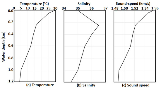
Figure 5.
Observed temperature and salinity data from the XBT and CTD deployments in the Gulf of Mexico. (a) Temperature; (b) salinity; (c) sound-speed calculated from the temperature and salinity values shown in (a,b), depth-dependent pressure calculated from Equation (6) assuming a constant density and no latitude correction, and Equation (5).

Figure 6.
(a) V versus T and (b) V versus S cross-plots. The plotted points are black dots, and the best-fit polynomials are red curves. The best-fit equations including their R2 values are also shown.
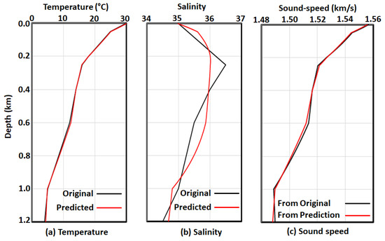
Figure 7.
Demonstration of the accuracy of Equation (9). (a) Temperature prediction, (b) salinity prediction, and (c) sound-speed prediction.
Figure 5a,b shows the (in ) and measurements from XBT and CTD deployments in the Gulf of Mexio area that are available in the public domain. Using these measurements, calculating from Equation (6) with kg/m3 and m/s2, we then used Equation (5) to calculate , which we show in Figure 5c (in km/s), illustrating that reasonable values of can be computed from and . Next, we attempted to express and , shown in Figure 5a,b as functions of , which is shown in Figure 5c. To do so, we cross-plotted both and as the vertical axes and as the horizontal axis and obtained best-fit polynomials through the plotted points. These cross-plots (in black dots) and best-fit polynomials (in red curves) are shown in Figure 6a,b, expressing and as
It must be noted from Figure 6 that is more accurate than . In addition, while the prediction of is unambiguous, there is an ambiguity in the prediction of , as the same value of can be predicted from two different values of (see Figure 6). This ambiguity is due to the nature of the temperature and salinity data that we obtained from the Gulf of Mexico. Both and decrease with depth (see Figure 1, Figure 2, Figure 3, Figure 4 and Figure 5). On the other hand, increases from the surface to a depth of about 200 m and then decreases (see Figure 5). Although these variations are uncommon, they were the only data we could find for our initial model. We will further discuss this issue in a later part of this paper.
To further illustrate the accuracy of and , shown by Equation (9), in Figure 7, we show the quality of our prediction. Figure 7a,b compares the predicted and in red with the original (observed) and of Figure 5a,b in black. And Figure 7c compares the sound-speeds. The black curve of Figure 7c is the same sound-speed shown in Figure 5c that we computed from the observed and (Figure 5a,b). On the other hand, we computed the red curve of Figure 7c from the predicted and (red curves of Figure 7a,b). Notice that, despite less accuracy and ambiguity in the prediction of , the sound-speeds can be predicted with reasonable accuracy. Therefore, from the seismically inverted sound-speeds, using Equation (9) will provide a reasonably good initial model of and for the ADAM optimization.
In our implementation of ADAM, we first define our model at any time step as
Clearly, for , our model is the initial model, which we compute from the inverted sound-speeds using Equation (9) for each depth sample . Having defined as above, we then use Equation (5) to compute the predicted sound-speed for time step , given as
Having computed , we then compute the objective as
In Equation (12), is the true sound-speed which we obtain from seismic inversion. In general, additional regularization parameters or weighting matrices are used in between the first and second terms on the right-hand side of Equation (12). The purpose of using these weighting matrices is to stabilize the optimization. In our implementation, however, we did not use them because these regularization parameters are built in to the ADAM optimization method, which we discuss below.
Finding the optimal model , with its components being the temperature and salinity values (Equation (4)) that predict the observed set of sound-speeds (Equation (3)), is a classical least square minimization problem that requires iteratively minimizing the objective . The ADAM algorithm achieves this minimization by using both the gradient of and its square. Although the details of the methodology can be found elsewhere [53], for completeness, we outline below the ADAM methodology for estimating and from .
We first compute the gradient of the objective, given as
Note that is a vector of -components containing the partial derivatives of each component of (Equation (11)) with respect to each component of (Equation (10)). For general optimization problems, these partial derivatives are numerically computed. However, for our problem of mapping onto and , these derivatives can be analytically computed, and in Appendix B, we derive the explicit forms of these derivatives and provide the analytical expression of .
After obtaining , we update the biased first order moment for the next time step from that of the current time step () as
Similarly, we update the biased second order moment from as
Like , , , , and are -component vectors, in Equation (15) is a component-wise square of . The parameters and are regularization parameters. For machine learning-related applications, well-tested default settings for these parameters are and [53]. For our implementation also, these default settings worked very well. Also, note from Equations (14) and (15) that both and are updated from and ; their corresponding values at the previous time step. In practice, for time step zero, and are set to null (zero) vectors so that Equations (14) and (15) can be used for subsequent updating. After updating the biased first- and second-order moments and , we then compute the bias-corrected first- and second-order moments and as
and
Finally, we obtain the updated model from
The parameter above is the step size and is another regularization term. For machine learning applications, the well-tested default values are and [53], and we used these default values in our implementation. Based on this discussion, Figure 8 is our implementation of the ADAM optimization to estimate and from , which is estimated from seismic inversion.
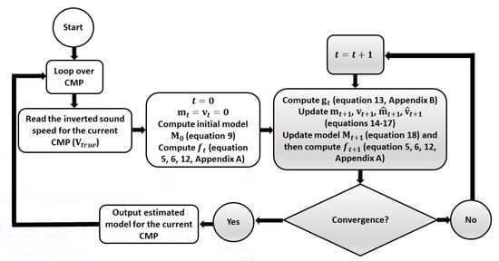
Figure 8.
Implementation of the ADAM optimization to estimate the temperature and salinity from the sound-speed estimated from seismic inversion. ADAM optimization modules are shaded in light gray.
As shown in Figure 8, we start with the loop over the CMP location. For each CMP, we first read the inverted sound-speed for all depth samples. We then set the time step and initialize the -component first- and second-order moments and to null vectors. We also use Equation (9) to compute the -component initial model vector . Next, we compute the objective . To compute , we first compute from using Equations (5) and (6), and additional equations provided in Appendix A. After computing , for time step zero, we enter the main ADAM optimization modules, shaded in light gray in Figure 8. First, we use Equation (13) and additional equations provided in Appendix B to compute , the gradient of the objective. Next, we use Equations (14) and (15) to update the biased first- and second-order moments and for the next time step from their values at the current time step. Following this, we compute the unbiased moments and from Equations (16) and (17) and use Equation (18) to update the model from . After obtaining the updated model for the next time step, we must decide whether to continue iterating or whether the updated model is sufficiently close to the true model so that we can exit, output the estimated model, and move onto the next CMP location. To do so, we compute the objective using the same procedure outlined above and check for convergence. The primary criterion for this convergence check is to find out whether the sound-speed , predicted from , is sufficiently close to . If it is, we exit iterating, output the model to be our best estimate of the temperature and salinity values, and move onto the next CMP location. On the other hand, if , predicted from , is not sufficiently close to , we continue iterating by setting as our current time step . In our implementation, we set this convergence check using two criteria: (1) the maximum number of iterations allowed and (2) the minimum root mean square error (RMSE) between and to be achieved. If either one of these two criteria is satisfied, then the method exits iterating, and otherwise, it continues iterating.
We first tested the validity of our method for a single location. We extracted the sound-speed values for CMP 9350, situated in the middle of Figure 4b, and used the methodology described by Figure 8 to estimate the temperature and salinity from the extracted sound-speed values. Figure 9 and Figure 10 show the results of this estimation. Starting from the initial values computed using Equation (9) (black curves in Figure 9a,b), we ran the ADAM optimization, and the final values of our estimation of temperature and salinity are shown as red curves in Figure 9a,b. To validate the accuracy of our estimation, in Figure 10 we compare the true sound-speed at CMP 9350 with the sound-speeds computed from Equation (5), using both the initial model and the final model. The true sound-speed is shown in red, and those computed from the initial and final models are shown, respectively, in black and green in Figure 10. Notice that the sound-speed computed from the final model falls right on top of the true sound-speed so closely that the true sound-speed in red is not visible in Figure 10. This comparison validates that our method can find the temperature and salinity from the sound-speed with a very good accuracy.
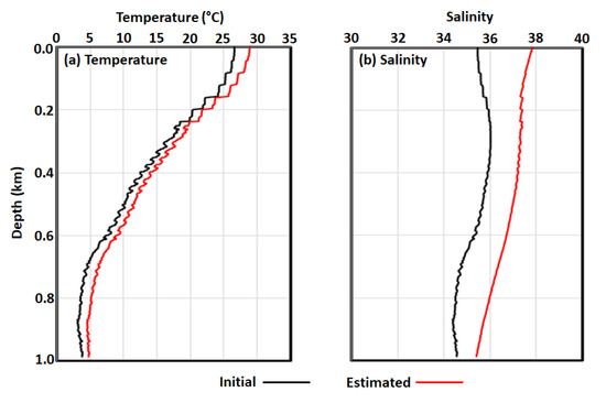
Figure 9.
Application of ADAM optimization at a single location, (a) temperature and (b) salinity. The initial models are in black, while the estimated models are in red.
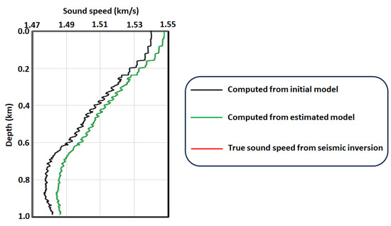
Figure 10.
Comparison of the true sound-speed model with those computed using the initial model, shown by the black curves in Figure 9, and final estimated model, shown by the red curves in Figure 9. Note that the sound-speed computed from the final estimated model is so close to the true model that the true model is completely invisible at the scale.
After validating the method at a single location, we applied our method to the entire domain of the inverted sound-speed data, shown in Figure 4b and Figure 11, which show the results of our estimation.
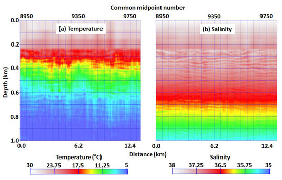
Figure 11.
(a) Temperature and (b) salinity, estimated by our method from the inverted sound-speed model shown in Figure 4b.
We further validate our estimation by computing the RMSE between the true sound-speed model of Figure 4b and the predicted sound-speed model computed from the initial and final estimated models. While the average RMSE between the true and initial models was about 12%, that between the true and inverted models was less than 0.001%. We also computed the sound-speed model using the final estimated model shown in Figure 11 and the equation of state (Equation (5)), and compared that with the true sound-speed model of Figure 4b. This predicted sound-speed was almost identical to the sound-speed model of Figure 4b, with a maximum difference of 0.0025 m/s between them, and is therefore not shown.
3. Discussion and Future Possibilities of Improvement
Our two-step approach to estimate the temperature and salinity from seismic data worked very well. The predicted sound-speeds computed from our estimated values of temperature and salinity match almost perfectly with their true values. We also compared our estimates with previous estimates [11] and verified that they reasonably match with one another. Primary advantages of our approach compared with the method used in these previous estimates [11] are its ease of use and computational efficiency. The attribute-guided approach to generate the initial model is fully automated and can even be obtained via shipboard processing. Although GA inversion is computer-intense, if shipboard computers are connected to a high-performance computing facility, then estimating sound-speeds is also feasible. Our proposed ADAM optimization is also computationally efficient. Estimating the temperature and salinity for the entire range of the 992 CMP locations shown in Figure 11 took about one hour to complete in a Linux workstation. Additionally, we did not make any attempt to parallelize our ADAM methodology. It is, however, clear from Figure 8 that the estimations of temperature and salinity for each CMP location are independent of one another. Consequently, it is not difficult to modify the method to simultaneously run on different CMP locations in a parallel computing environment, which can further enhance its computational efficiency. Therefore, with network connectivity to a high-performance computing facility, it may be possible to obtain real-time shipboard estimates of temperature and salinity using our method.
It is also important to point out the derivation of the initial models that we used in our estimation of temperature and salinity. From a few measured values from the Gulf of Mexico, we derived the and relations (Equation (9)) and used them to obtain our initial temperature and salinity models from the seismic sound-speeds from an entirely different region of the world. And yet, starting from this initial model, our method successfully obtained reasonable estimates of temperature and salinity. We previously pointed out, while discussing these initial models, that there is an ambiguity in our relation because the same value of is obtainable from two different values of (see the red curve in Figure 6b). To investigate how this ambiguity could affect our estimates, we carried out additional sensitivity analyses and show them in Figure 12. As shown in this figure, we computed the six sets of sound-speed models using Equations (5) and (6) as follows:
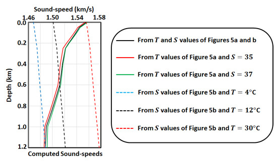
Figure 12.
Sensitivity analysis of the computed sound-speed to different values of temperature and salinity.
- Using the measured values of Figure 5a and a constant value of (solid red curve);
- Using the measured values of Figure 5a and a constant value of (solid green curve);
- Using the measured values of Figure 5b and a constant (dashed blue curve);
- Using the measured values of Figure 5b and a constant (dashed black curve);
- Using the measured values of Figure 5b and a constant .
Several inferences can be drawn from the results shown in Figure 12, such as:
- is more sensitive to the variations in than ;
- For a fixed , increases with ;
- For a fixed , increases with ;
- It is that primarily controls the shape of how varies with depth, and only provides bulk-shifts to their estimates.
Because controls the shape of and only provides a bulk-shift, despite the ambiguity in the estimation of shown in Equation (9) and Figure 6b, we believe that our results are accurate. We must, however, note that, because is more sensitive to the variations in than those in , the uncertainty in our estimation of is likely to be higher than that of . Additionally, although using an initial model derived from data from the Gulf of Mexico worked well on the data from the South China Sea, this does not necessarily imply that this model can be used as the initial model to invert any marine seismic data. The primary motivation of our current work is to demonstrate the applicability of our two-step method. In practice, the initial model must be site-specific and should be preferably derived from the XBT and CTD. Quantifying the uncertainties of our and estimations and the applicability of our two-step process to other marine seismic data is currently being investigated.
Finally, above, we argued that it is feasible to apply our proposed method shipboard such that and could be estimated in real time. This possibility, however, requires network connectivity to a high-performance computing facility. Although feasible, we must point out that GA inversion is computationally demanding [11,45]. Replacing GA with a more computationally efficient gradient-based local method can improve computational efficiency. However, due to the inherent non-uniqueness of the seismic inverse problems, it has been demonstrated that the GA provides much superior sound-speed estimates to the local methods and should be the preferred choice [11]. Therefore, seeking means to further improve the computational efficiency of the method is desirable. In recent years, the use of artificial intelligence (AI) and specifically machine learning (ML) methods revolutionized almost all fields of science and engineering. We believe that physics-informed machine learning (PIML) [58,59,60,61,62,63,64,65,66,67,68,69], a recent advancement in supervised learning for ML, can modify our two-step approach to a single step and further improve the computational efficiency. The standard practice for the supervised learning for ML is to use the labelled data for training and adjusting the network weights. Instead of using labelled data, PIML utilizes the underlying physics of the problem as the primary network driver. By using the underlying physics, PIML has been demonstrated to work very well for seismic inverse problems, in terms of improving both computational efficiency and the accuracy of the estimated model as compared with a standard ML approach using the labelled data for supervised learning [62]. In Figure 13, we provide our vision of how PIML can modify our two-step approach into a single step and improve computational efficiency. By feeding the seismic data at selected locations from the input layer into a deep learning architecture, we will directly predict the temperature and salinity. Then, by computing pressure from Equation (6), we will use Equation (5) to compute the sound-speed model. Using this sound-speed model and assuming a constant density, we will then use the physics of the problem (wave equation-based method) and compute synthetic (predicted) seismic data. For learning, we will then iteratively adjust the network weights by matching these synthetic seismic data with the true seismic data until convergence. Once learning is complete, we can then use our trained network to directly predict the temperature and salinity from the entire seismic data. Although connectivity to a high-performance parallel computing facility would be necessary for training (learning), we expect that this PIML approach can improve the overall computational efficiency and be used for the real-time shipboard prediction of temperature and salinity directly from the acquired seismic data. Implementation of the overall concept of Figure 13 is currently being investigated and will be discussed in a separate paper.
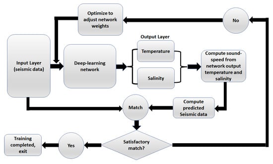
Figure 13.
The overall concept of a PIML-based approach to directly predict temperature and salinity from marine seismic data.
4. Conclusions
We propose a two-step process to estimate temperature () and salinity () from marine seismic reflection data. The method is fully automated and does not require any human intervention such as careful inversion runs at sparse locations, manually interpreting horizons, or interpolating sparsely inverted models in-between the interpreted horizons. Subject to network connectivity to a high-performance computing facility, it is also feasible make real-time shipboard estimations of and using our method. Additionally, we also discuss how the computational efficiency of the method can be further improved using a PIML approach of directly predicting and from seismic data in a single step. Although the vertical resolution is low, our seismically estimated and are of much higher lateral resolution than those obtainable from the XBT and CTD deployments in the oceans. We therefore believe that estimating and using our two-step method or its improvedSo single-step PIML version can impact the future of weather prediction, climate modeling, and marine biology research.
Author Contributions
Conceptualization, S.M.; Methodology, D.C.; Software, D.C.; validation, D.C.; formal analysis, D.C.; investigation, D.C.; resources, S.M.; data curation, D.C.; writing—original draft preparation, D.C.; writing—review and editing, S.M.; visualization, D.C.; supervision, S.M.; project administration, S.M.; funding acquisition, S.M. All authors have read and agreed to the published version of the manuscript.
Funding
This research received no external funding.
Institutional Review Board Statement
This study did not require any ethical approval.
Informed Consent Statement
Not applicable.
Data Availability Statement
All data shown in this research can be available by contacting the corresponding author.
Acknowledgments
We acknowledge the use of computational resources at the Advanced Research Computing Center (ARCC) of the University of Wyoming (https://doi.org/10.15786/M2FY47) and the NCAR Wyoming Supercomputing Center provided by the National Science Foundation and the State of Wyoming and supported by NCAR’s Computational and Information Systems Laboratory (https://doi.org/10.5065/D6RX99HX). We also thank three anonymous reviewers whose constructive comments substantially improved the quality of the manuscript.
Conflicts of Interest
The authors declare no conflicts of interest.
Appendix A. Sound-Speed Calculation
For any depth sample , Equation (5) provides the sound-speed as a function of the temperature , salinity , and pressure . This equation is one of many equations of state relating different oceanwater physical properties with one another [41,42,43]. The coefficients , , , and in Equation (5) are given as
and
In Equations (A1)–(A4), the coefficients , , , and are constants and their values are provided in Table A1.

Table A1.
Values of the coefficients , , , and in Equations (A1)–(A4).
Table A1.
Values of the coefficients , , , and in Equations (A1)–(A4).
| Coefficient | Value | Coefficient | Value |
|---|---|---|---|
| C00 | 1402.388 | A02 | 7.166 × 10⁻⁵ |
| C01 | 5.0383 | A03 | 2.008 × 10⁻⁶ |
| C02 | −0.05819 | A04 | −3.21 × 10⁻⁸ |
| C03 | 3.3432 × 10⁻⁴ | A10 | 9.4742 × 10⁻⁵ |
| C04 | −1.47797 × 10⁻⁶ | A11 | −1.2583 × 10⁻⁵ |
| C05 | 3.1419 × 10⁻⁹ | A12 | −6.4928 × 10⁻⁸ |
| C10 | 0.153563 | A13 | 1.0515 × 10⁻⁸ |
| C11 | 6.8999 × 10⁻⁴ | A14 | −2.0142 × 10⁻¹⁰ |
| C12 | −8.1829 × 10⁻⁶ | A20 | −3.9064 × 10⁻⁷ |
| C13 | 1.3632 × 10⁻⁷ | A21 | 9.1061 × 10⁻⁹ |
| C14 | −6.126 × 10⁻¹⁰ | A22 | −1.6009 × 10⁻¹⁰ |
| C20 | 3.126 × 10⁻⁵ | A23 | 7.994 × 10⁻¹² |
| C21 | −1.7111 × 10⁻⁶ | A30 | 1.10 × 10⁻¹⁰ |
| C22 | 2.5986 × 10⁻⁸ | A31 | 6.651 × 10⁻¹² |
| C23 | −2.5353 × 10⁻¹⁰ | A32 | −3.391 × 10⁻¹³ |
| C24 | 1.0415 × 10⁻¹² | B00 | −1.922 × 10⁻² |
| C30 | −9.7729 × 10⁻⁹ | B01 | −4.42 × 10⁻⁵ |
| C31 | 3.8513 × 10⁻¹⁰ | B10 | 7.3637 × 10⁻⁵ |
| C32 | −2.3654 × 10⁻¹² | B11 | 1.795 × 10⁻⁷ |
| A00 | 1.389 | D00 | 1.727 × 10⁻³ |
| A01 | −1.262 × 10⁻² | D10 | −7.9836 × 10⁻⁶ |
Thus, by computing the pressure from Equation (6), it is straightforward to use Equation (5) and Equations (A1)–(A4) along with the values of the coefficients , , , and provided in Table A1 and compute the sound-speed from and for any depth sample . The accuracy of Equation (5) in computing using this procedure is m/s [42].
Appendix B. Analytical Expression of the Gradient of the Objective
Updating the model for time step to for time step , the ADAM optimization requires defining the objective (Equation (12)) and computing its gradient (Equation (13)). Although we described the governing equations (Equations (14)–(18)) and the implementation details of the method (Figure 8), we did not discuss how to compute . Here, we derive the equations for the analytical expression of for mapping onto and .
As before, we use to be our true sound-speed model from seismic inversion with depth samples. However, for consistency, instead of defining the predicted sound-speed, computed from at time step as , we define it as . We also remove the subscript in the definition of the objective and rewrite Equation (12) as
In Equation (A5), and denote the sample of and . From Equation (A5), we can write the gradient of the objective as
In Equation (A6) and have the same meaning as they have in Equation (A5). The parameters and respectively denote the sample of the temperature and salinity model for the current time step . In other words, they are the and sample of the -component model vector (see Equation (10)).
It is thus clear from Equation (A6) that if we can get explicit expressions for and for all depth samples , we then have the analytical expression for the gradient . Note that deriving the explicit expressions of and for sample is not different from another sample . Additionally, the subscript for the sound-speed and in the temperature and salinity used in Equation (A5) respectively stand for the predicted sound-speed values and the current time step. For convenience, we may therefore ignore these subscripts and superscripts and replace and by and , keeping the following facts in mind:
- is the predicted sound-speed for a given sample of the component predicted sound-speed vector at the current time step ;
- and are the current values of temperature and salinity for two corresponding samples of the component model vector at the current time step .
Using the above conventions, we can derive the partial derivatives and from Equation (5) as
and
In addition, from Equations (A1)–(A4), we can also write
and
Equations (A7)–(A11), in association with the coefficients , , , and given in Table A1, provide explicit analytical expressions for the partial derivatives and . Or to be explicit, they provide the analytical expressions for and for any time sample for the time step . These analytical expressions, for each sample, when substituted onto Equation (A6), provides the exact analytical expression of the gradient of the objective for the given time step.
References
- Thorpe, S.A. The Turbulent Ocean; Cambridge University Press: Cambridge, UK, 1967. [Google Scholar] [CrossRef]
- Meredith, M.P.; King, J.C. Rapid climate change in the ocean west of the Antarctic Peninsula during the second half of the 20th century. Geophys. Res. Lett. 2005, 32, 1–5. [Google Scholar] [CrossRef]
- Durac, P.J.; Wijffels, S.E.; Matear, R.J.; Durac, P.J.; Wijffels, S.E.; Matear, R.J. Ocean Salinities Reveal Strong Global Water Cycle Intensification During 1950 to 2000. Science 2012, 336, 455–458. [Google Scholar] [CrossRef] [PubMed]
- Bender, M.A.; Knutson, T.R.; Tuleya, R.E.; Sirutis, J.J.; Vecchi, G.A.; Garner, S.T.; Held, I.M. Modeled Impact of Anthropogenic Warming on the Frequency of Intense Atlantic Hurricanes. Science 2010, 327, 454–458. [Google Scholar] [CrossRef] [PubMed]
- Castillo, J.; Basrbieri, M.A.; Gonzalez, A. Relationships between sea surface temperature, salinity, and pelagic fish distribution off northern Chile. ICES J. Mar. Sci. 1996, 53, 139–146. [Google Scholar] [CrossRef]
- Rijnsdorp, A.D.; Peck, M.A.; Engelhard, G.H.; Möllmann, C.; Pinnegar, J.K. Resolving the effect of climate change on fish populations. ICES J. Mar. Sci. 2009, 66, 1570–1583. [Google Scholar] [CrossRef]
- Brucet, S.; Boix, D.; Nathansen, L.W.; Quintana, X.D.; Jensen, E.; Balayla, D.; Meerhoff, M.; Jeppesen, E. Effects of Temperature, Salinity and Fish in Structuring the Macroinvertebrate Community in Shallow Lakes: Implications for Effects of Climate Change. PLoS ONE 2012, 7, e30877. [Google Scholar] [CrossRef]
- Sugie, K.; Fugiwara, A.; Nishino, S.; Kameyayama, A.; Harada, N. Impacts of Temperature, CO2, and Salinity on Phytoplankton Community Composition in the Western Arctic Ocean. Front. Mar. Sci. 2020, 6, 821. [Google Scholar] [CrossRef]
- Smith, D.M.; Murphy, J.M. An objective ocean temperature and salinity analysis using covariances from a global climate model. J. Geophys. Res. 2006, 112, 1–19. [Google Scholar] [CrossRef]
- Levitus, S.; Gelfeld, T.; Boyer, T.; Johnson, D. Results of the NODC and IOC, Oceanographic Data Archaeology and Rescue Projects, Key to Oceanographic Records and Documentation No. 19; NODC: Washington, DC, USA, 1994. Available online: https://repository.library.noaa.gov/view/noaa/17356 (accessed on 6 February 2024).
- Padhi, A.; Mallick, S.; Fortin, W.; Holbrook, W.S.; Blacic, T.M. 2-D ocean temperature and salinity images from pre-stack seismic waveform inversion methods: An example from the South China Sea. Geophys. J. Int. 2015, 202, 800–810. [Google Scholar] [CrossRef]
- Holbrook, W.; Páramo, P.; Pearse, S.; Schmitt, R.W. Thermohaline fine structure in an oceanographic front from seismic reflection profiling. Science 2003, 821–824. [Google Scholar] [CrossRef]
- Tsuji, T.; Noguchi, T.; Niino, H.; Matsuoka, T.; Nakamura, Y.; Tokuyama, H.; Kuramoto, S.; Bangs, N. Two-dimensional mapping of fine structures in the Kuroshio Current using seismic reflection data. Geophys. Res. Lett. 2005, 32, L14609. [Google Scholar] [CrossRef]
- Nakamura, Y.; Noguchi, T.; Tsuji, T.; Itoh, S.; Niino, H.; Matsuoka, T. Simultaneous seismic reflection and physical oceanographic observations of oceanic fine structure in the Kuroshio extension front. Geophys. Res. Lett. 2006, 33, L23605. [Google Scholar] [CrossRef]
- Biescas, B.; Ruddick, B.R.; Nedimovic, M.R.; Sallares, V.; Bornstein, G.; Mojica, J.F. Recovery of temperature, salinity, and potential density from ocean reflectivity. J. Geophys. Res. Ocean. 2014, 119, 3171–3184. [Google Scholar] [CrossRef]
- Ruddick, B.; Song, H.B.; Dong, C.Z.; Pinheiro, L. Water column seismic images as maps of temperature gradient. Oceanography 2009, 22, 192–205. [Google Scholar] [CrossRef]
- Sheen, K.L.; White, N.J.; Hobbs, R.W. Estimating mixing rates from seismic images of oceanic structure. Geophys. Res. Lett. 2009, 36, L00D04. [Google Scholar] [CrossRef]
- Fortin, W.F.; Holbrook, W.S.; Schmitt, R.W.; Smith, S. Mapping non-local turbulent breakdown of oceanic lee waves offshore Costa Rica through seismic oceanography. Proc. Meet. Acoust. 2013, 19, 005014. [Google Scholar] [CrossRef]
- Holbrook, W.S.; Fer, I.; Schmitt, R.W.; Lizarralde, D.; Klymak, J.M.; Helfrich, L.C.; Kubichek, R. Estimating oceanic turbulence dissipation from seismic images. J. Atmos. Ocean. Technol. 2013, 30, 1767–1788. [Google Scholar] [CrossRef]
- Klaeschen, D.; Hobbs, R.W.; Krahmann, G.; Papenberg, C.; Vsemirnova, E. Estimating movement of reflectors in the water column using seismic oceanography. Geophys. Res. Lett. 2009, 36, L00D03. [Google Scholar] [CrossRef]
- Huang, X.; Song, H.; Bai, Y.; Chen, J.; Liu, B. Estimation of seawater movement based on reflectors from a seismic profile. Acta Oceanol. Sin. 2012, 31, 46–53. [Google Scholar] [CrossRef]
- Fortin, W.F.J.; Holbrook, W.S. Sound speed requirements for optimal imaging of seismic oceanography data. Geophys. Res. Lett. 2009, 36, L00D01. [Google Scholar] [CrossRef]
- Blacic, T.M.; Holbrook, W.S. First images and orientation of fine structure from a 3D seismic oceanography data set. Ocean Sci. 2010, 6, 431–439. [Google Scholar] [CrossRef]
- Páramo, P.; Holbrook, W.S. Temperature contrasts in the water column inferred from amplitude versus offset analysis of acoustic reflections. Geophys. Res. Lett. 2005, 32, L24611. [Google Scholar] [CrossRef]
- Papenberg, C.; Klaeschen, D.; Krahmann, G.; Hobbs, R.W. Ocean temperature and salinity inverted from combined hydrographic and seismic data. Geophys. Res. Lett. 2010, 37, 1–6. [Google Scholar] [CrossRef]
- Wood, W.T.; Holbrook, W.S.; Sen, M.K.; Stoffa, P.L. Full waveform inversion of reflection seismic data for ocean temperature profiles. Geophys. Res. Lett. 2008, 35, L04608. [Google Scholar] [CrossRef]
- Kormann, J.; Biescas, B.; Korta, N.; de la Puente, J.; Sallarès, V. Application of acoustic full waveform inversion to retrieve high-resolution temperature and salinity profiles from synthetic seismic data. J. Geophys. Res. 2011, 116, 1–14. [Google Scholar] [CrossRef]
- Song, H.B.; Huang, X.H.; Pinheiro, L.M.; Song, Y.; Dong, C.Z.; Bai, Y. Inversion studies in seismic oceanography. In Computational Methods for Applied Inverse Problems, Chapter 16; Wang, Y., Yagola, A.G., Yang, C., Eds.; De Gruyter: Berlin, Germany; Boston, MA, USA, 2012; pp. 395–410. [Google Scholar] [CrossRef]
- Bornstein, G.; Biescas, B.; Sallarès, V.; Mojica, J.F. Direct temperature and salinity acoustic full waveform inversion. Geophys. Res. Lett. 2013, 40, 4344–4348. [Google Scholar] [CrossRef]
- Blacic, T.M.; Jun, H.; Rosado, H.; Shin, C. Smooth 2-D ocean sound speed from Laplace and Laplace-Fourier domain inversion of seismic oceanography data. Geophys. Res. Lett. 2016, 43, 1211–1218. [Google Scholar] [CrossRef]
- Dagnino, D.; Sallarès, V.; Biescas, B.; Ranero, C.R. Fine-scale thermohaline ocean structure retrieved with 2-D prestack full-waveform inversion of multichannel seismic data: Application to the Gulf of Cadiz (SW Iberia). J. Geophys. Res. Ocean. 2016, 121, 5452–5469. [Google Scholar] [CrossRef]
- Dagnino, D.; Sallarès, V.; Ranero, C.R. Waveform-preserving processing flow of multichannel seismic reflection data for Adjoint-State Full waveform inversion of ocean Thermohaline Structure. IEEE Trans. Geosci. Remote Sen. 2018, 56, 1615–1625. [Google Scholar] [CrossRef]
- Minakov, A.; Keers, H.; Kolyukhin, D.; Tengesdal, H.C. Acoustic waveform inversion for ocean turbulence. J. Phys. Oceanogr. 2017, 47, 1473–1491. [Google Scholar] [CrossRef]
- Gunn, K.L.; White, N.; Caulfield, C.P. Time-Lapse seismic imaging of oceanic fronts and transient lenses within South Atlantic Ocean. J. Geophys. Res. Ocean. 2020, 125, e2020JC016293. [Google Scholar] [CrossRef]
- Gunn, K.L.; White, N.J.; Larter, R.D.; Caulfield, C.P. Calibrated seismic imaging of eddy-dominated warm-water transport across the Bellingshausen Sea, Southern Ocean. J. Geophys. Res. Ocean. 2018, 123, 3072–3099. [Google Scholar] [CrossRef]
- Tang, Q.; Hobbs, R.; Zheng, C.; Biescas, B.; Caiado, C. Markov Chain Monte Carlo inversion of temperature and salinity structure of an internal solitary wave packet from marine seismic data. J. Geophys. Res. Ocean. 2016, 121, 3692–3709. [Google Scholar] [CrossRef]
- Azevedo, L.; Huang, X.; Pinheiro, L.M.; Nunes, R.F.M.; Caeiro, M.H.; Song, H.; Soares, A. Geostatistical inversion of seismic oceanography data for ocean salinity and temperature models. Math. Geosci. 2018, 50, 477–489. [Google Scholar] [CrossRef]
- Azevedo, L.; Matias, L.; Turco, F.; Tromm, R.; Peliz, A. Geostatistical seismic inversion for temperature and salinity in the Madeira Abyssal Plain. Front. Mar. Sci. 2021, 8, 685007. [Google Scholar] [CrossRef]
- Jun, H.; Cho, Y.; Noh, J. Trans-dimensional Markov chain Monte Carlo inversion of sound speed and temperature: Application to yellow sea multichannel seismic data. J. Mar. Syst. 2019, 197, 103180. [Google Scholar] [CrossRef]
- Chhun, C.; Tsuji, T. Sound speed of thermohaline fine structure in the Kuroshio Current inferred from automatic sound speed analysis. Expl. Geophys. 2020, 51, 581–590. [Google Scholar] [CrossRef]
- Chen, C.T.; Millero, F.J. Speed of sound in seawater at high pressures. J. Acoust. Soc. Am. 1977, 62, 1129–1135. [Google Scholar] [CrossRef]
- Fofonoff, P.; Millard, R.C., Jr. Algorithms for Computation of Fundamental Properties of Seawater; UNESCO Technical Papers in Marine Sciences No. 44; UNESCO: Paris, France, 1983; 53p. [Google Scholar] [CrossRef]
- Wong, G.S.K.; Zhu, S. Speed of sound in seawater as a function of salinity, temperature and pressure. J. Acoust. Soc. Am. 1995, 97, 1732–1736. [Google Scholar] [CrossRef]
- Leroy, C.C.; Parthiot, F. Depth-pressure relationship in the oceans and seas. J. Acoust. Soc. Am. 1998, 103, 1346–1352. [Google Scholar] [CrossRef]
- Mallick, S.; Chakraborty, D. Prediction of the ocean water sound speeds via attribute-guided seismic waveform inversion. Geophysics 2002, 87, U67–U79. [Google Scholar] [CrossRef]
- Tarantola, A. Inverse Problem Theory and Methods for Model Parameter Estimation; The Society of Industrial and Applied Mathematics: Philadelphia, PA, USA, 2005; ISBN 0-89871-572-5. [Google Scholar]
- Mallick, S. Model-based inversion of amplitude-variations-with-offset data using a genetic algorithm. Geophysics 1995, 60, 939–954. [Google Scholar] [CrossRef]
- Mallick, S. Some practical aspects of prestack waveform inversion using a genetic algorithm: An example from the east Texas Woodbine gas sand. Geophysics 1999, 64, 326–336. [Google Scholar] [CrossRef]
- Mallick, S.; Adhikari, S. Amplitude-variation-with-offset and prestack waveform inversion: A direct comparison using a real data example from the Rock Springs Uplift, Wyoming, USA. Geophysics 2015, 80, B45–B59. [Google Scholar] [CrossRef]
- Huck, A.; Quiquerez, G.; de Groot, P. Improving seismic inversion through detailed low frequency model building. In Proceedings of the 72nd EAGE Conference and Exhibition (Expanded Abstract), Barcelona, Spain, 14–17 June 2010. [Google Scholar] [CrossRef]
- Pafeng, J.; Mallick, S.; Sharma, H. Prestack waveform inversion of three-dimensional seismic data — An example from the Rock Springs Uplift, Wyoming, USA. Geophysics 2017, 82, B1–B12. [Google Scholar] [CrossRef]
- Lau, A.; Gonzalez, A.; Mallick, S.; Gillespie, D. Waveform gather inversion and attribute-guided interpolation: A two-step approach to log prediction. Lead. Edge 2002, 21, 1024–1027. [Google Scholar] [CrossRef]
- Kingma, D.P.; Ba, J.L. ADAM: A method for stochastic optimization. arXiv 2014, arXiv:1412.6980. [Google Scholar] [CrossRef]
- Yilmaz, Ö. Seismic Data Processing; Society of Exploration Geophysicists: Tulsa, OK, USA, 1989; ISBN 978-1560800941. [Google Scholar]
- Kuremoto, T.; Furuya, M.; Mabu, S.; Kobayashi, K. A Time Series Forecasting Method Using DBN and Adam Optimization. In Proceedings of the International Conference on Artificial Intelligence for Communications and Networks, Hiroshima, Japan, 1–30 November 2022; pp. 95–106. [Google Scholar] [CrossRef]
- William, L. Fundamentals of Geophysics, 2nd ed.; Cambridge University Press: Cambridge, UK, 2012. [Google Scholar] [CrossRef]
- Moritz, H. Geodetic reference system. Bull. Géodésique 1980, 54, 395–405. [Google Scholar] [CrossRef]
- Raissi, M.; Perdikaris, P.; Karniadakis, G.E. Physics Informed Deep Learning (Part I): Data-Driven Solut. Nonlinear Partial Differ. Equations. arXiv 2017, arXiv:1711.10561v1. [Google Scholar]
- Raissi, M.; Yazdani, A.; Karniadakis, G.E. Hidden Fluid Mechanics: A Navier–Stokes Informed Deep Learning Framework for Assimilating Flow Visualization Data. arXiv 2018, arXiv:1808.04327v1. [Google Scholar]
- Raissi, M.; Perdikaris, P.; Karniadakis, G.E. Physics-informed neural networks: A deep learning framework for solving forward and inverse problems involving nonlinear partial differential equations. J. Comput. Phys. 2019, 378, 686–707. [Google Scholar] [CrossRef]
- Raissi, M.; Yazdani, A.; Karniadakis, G.E. Hidden fluid mechanics: Learning velocity and pressure fields from flow visualizations. Science 2020, 367, 1026–1030. [Google Scholar] [CrossRef] [PubMed]
- Biswas, R.; Sen, M.K.; Das, V.; Mukerji, T. Prestack and poststack inversion using a physics-guided convolutional neural network. Interpretation 2019, 7, SE161–SE174. [Google Scholar] [CrossRef]
- Stefano, M. Physics-Informed Deep-Learning for Scientific Computing. arXiv 2021, arXiv:2103.09655v2. [Google Scholar]
- Dwivedi, V.; Parashar, N.; Srinivasan, B. Distributed learning machines for solving forward and inverse problems in partial differential equations. Neurocomputing 2021, 420, 299–316. [Google Scholar] [CrossRef]
- De Florio, M.; Schiassi, E.; Ganapol, B.D.; Roberto, F. Physics-informed neural networks for rarefied-gas dynamics: Thermal creep flow in the Bhatnagar–Gross–Krook approximation. Phys. Fluids 2021, 33, 047110. [Google Scholar] [CrossRef]
- Mishra, S.; Roberto, M. Estimates on the generalization error of physics-informed neural networks for approximating a class of inverse problems for PDEs. IMA J. Numer. Anal. 2022, 42, 981–1022. [Google Scholar] [CrossRef]
- Ali, K.; Mukerji, T. Physics-informed PointNet: A deep learning solver for steady-state incompressible flows and thermal fields on multiple sets of irregular geometries. J. Comput. Phys. 2022, 468, 111510. [Google Scholar] [CrossRef]
- Ryck, T.D.; Jagtap, A.D.; Mishra, S. Error estimates for physics informed neural networks approximating the Navier–Stokes equations. IMA J. Numer. Anal. 2023, 44, 83–119. [Google Scholar] [CrossRef]
- Fu, J.; Xiao, D.; Fu, R.; Li, C.; Zhu, C.; Arcucci, R.; Navon, I.M. Physics-data combined machine learning for parametric reduced-order modelling of nonlinear dynamical systems in small-data regimes. Comput. Methods Appl. Mech. Eng. 2023, 404, 115771. [Google Scholar] [CrossRef]
Disclaimer/Publisher’s Note: The statements, opinions and data contained in all publications are solely those of the individual author(s) and contributor(s) and not of MDPI and/or the editor(s). MDPI and/or the editor(s) disclaim responsibility for any injury to people or property resulting from any ideas, methods, instructions or products referred to in the content. |
© 2024 by the authors. Licensee MDPI, Basel, Switzerland. This article is an open access article distributed under the terms and conditions of the Creative Commons Attribution (CC BY) license (https://creativecommons.org/licenses/by/4.0/).