Abstract
Resistance serves as a critical performance metric for ships. Swift and accurate resistance prediction can enhance ship design efficiency. Currently, methods for determining ship resistance encompass model tests, estimation techniques, and computational fluid dynamics (CFDs) simulations. There is a need to improve the prediction speed or accuracy of these methods. Machine learning is gradually emerging as a method applied in the field of ship research. This study aims to investigate ship resistance prediction methods utilizing machine learning across various datasets. This study proposes two methods: employing stacking ensemble learning to enhance resistance prediction accuracy with identical ship samples and utilizing various ship resistance prediction models for accurate resistance prediction through transfer learning. Initially focusing on container ships as the research subject, the stacking ensemble learning model outperforms the basic machine learning model, the Holtrop and Mennen method, and the updated Guldhammer and Harvald method based on comparative prediction results. Subsequently, the container ship resistance prediction model achieves precise resistance prediction for bulk carriers. This study offers dependable guidance for applying machine learning in predicting ship hydrodynamic performance.
1. Introduction
As one of the paramount performance aspects of ships, resistance necessitates prioritization in ship design. It holds significant importance in the research of ship resistance prediction methods.
After over a century of research, model tests, estimation methods, and computational fluid dynamics (CFDs) simulations have emerged as three commonly employed approaches for determining ship resistance. Model tests, being the initial method employed for ship resistance prediction, are esteemed for their reliability. However, the outcomes of model tests can be influenced by various factors, including model geometry and test installation. ITTC gives recommended procedures and guidelines for model tests [1]. Estimation methods encompass a range of techniques such as standard series, Ayre, Lap–Keller, admiralty coefficient, statistical regression, and empirical equations. These methods are developed utilizing data from both model tests and actual ship sailing. Each estimation method is tailored to suit different ship types. Savitsky’s [2] method is suitable for calculating resistance in planning chine ships. The resistance of displacement ships can be calculated using the Hollenbach [3] and Holtrop and Mennen [4] methods. Calisal and Dan [5] proposed a resistance calculation method for smaller displacement ships with a small length/breadth ratio. Robinson [6] proposed a resistance calculation method for planning chine and round-bilge ships. These estimation methods have still been commonly used in recent years [7,8,9,10]. Some older estimation equations are updated with newer ship data. Kristensen and Bingham [11] proposed an updated Guldhammer and Harvald method based on the model tests of newer ships. Tu et al. [12] modified the admiralty coefficient to estimate power curves in EEDI calculations accurately. Crudu et al. [13] modified the bulb immersion in the Holtrop and Mennen method to estimate the resistance of a 3700 dwt chemical tanker. CFDs simulations offer a viable alternative to towing tank tests [14] and are widely used in ship resistance prediction [15,16,17,18]. The factors that affect the CFDs calculation results are computational grids, turbulence models, etc. Recommended procedures and guidelines for ship CFDs applications are also given by the ITTC [19].
Everything is a double-edged sword. Ngoc Vu Minh et al. [20] mentioned that model tests can yield reliable data, but they are time-consuming and expensive and usually performed at the end of the design cycle. Resistance can be rapidly obtained using estimation methods, but the accuracy is low. CFDs methods require high computer resources, especially for high-precision results and cases where there are many examples to calculate. Ravenna Roberto et al. [21] went through a lot of tedious computer calculations when using the StarCCM+ software (version 12.02.011-R8) to investigate the heterogeneous hull roughness effect on ship resistance. Both estimation methods and CFDs methods find common use in ship design. The rapid prediction capability of CFDs methods is contingent upon the advancement of computer technology. Meanwhile, improving the prediction accuracy of estimation methods remains challenging, constrained by the availability of data and expression methods.
The objective of this study is to identify a rapid and accurate method for predicting resistance using machine learning (ML). ML exhibits a robust capability to address nonlinear and complex problems. Numerous scholars have extensively researched ship resistance prediction using ML algorithms. Margari et al. [22] used an artificial neural network to predict the resistance of a series of ships designed according to the MARAD system. The results show that the multi-layer perceptron network model can be used to predict ship resistance. Using an artificial neural network, Cepowski [23] established a prediction model for ship-added resistance. The trained neural network was presented as the form of a mathematical function. Yildiz Burak [24] trained the neural network model using experimental data from a trimaran model in order to develop a more reliable model. Ivana Martić et al. [25] built a numerical model based on the results of hydrodynamic calculations in head waves, which can estimate the added resistance of container ships with sufficient accuracy. They [26] also used an artificial neural network to predict the added resistance coefficient for container ships in regular head waves for various speeds. Mentes Ayhan et al. [27] chose an artificial neural network (ANN) and an adaptive neuro-fuzzy inference system (ANFIS) as soft computation techniques to estimate the hawser tensions and displacements of a spread mooring system and compared the results of the two methods. Ozsari Ibrahim [28] uses an artificial neural network (ANN) model to predict the main engine power and pollutant emissions of container, cargo, and tanker ships. Yang et al. [29] also studied the performances of different ML algorithms on the resistance prediction of a container ship. Elik et al. [30] proposed a data-driven hull shape optimization method and used machine learning to establish a ship resistance prediction model.
Currently, research on the application of machine learning (ML) algorithms in ship resistance prediction is inadequate. Firstly, basic ML algorithms are more commonly utilized than complex ones, yet the prediction outcomes of these basic algorithms require enhancement. Additionally, ensemble learning, which enhances the ability to generalize systems, is seldom employed. Secondly, each prediction problem is treated in isolation, necessitating a large volume of data to achieve accurate forecasting results, thus increasing the modeling complexity. Transfer learning, which can achieve precise prediction outcomes with a limited sample size based on previous knowledge or prediction models, is also underutilized.
This study researches ship resistance prediction utilizing stacking ensemble learning and transfer learning. Two estimation methods, the Holtrop and Mennen and the updated Guldhammer and Harvald, are employed for comparison. The study is divided into two main parts. In the first part, four representative models—linear regression (LR), k-nearest neighbor (KNN), support vector regression (SVR), and random forest (RF)—are selected as basic machine learning (ML) models. Stacking ensemble models are then constructed using these basic models. The prediction results for container ship resistance are obtained and compared across basic ML models, stacking ensemble models, and the two estimation methods. In the second part, stacking ensemble learning models utilized for container ship resistance prediction are repurposed to predict the resistance of a bulk carrier using transfer learning. The prediction results for the bulk carrier using different methods are compared.
This study is structured into four sections.
Section 2 introduces the ship data of various vessels, including the KRISO container ship (KCS), 1100-TEU, 4250-TEU, 4700-TEU, 9000-TEU, and 13,500-TEU container ships, as well as a 47,500 dwt bulk carrier utilized in this research. Additionally, it outlines the definitions of basic machine learning (ML) models, stacking ensemble learning models, transfer learning models, and estimation methods, as well as elaborates on the training process of different models.
Section 3 presents the prediction results for both container ships and the 47,500 dwt bulk carrier using different methods. Furthermore, it analyzes the similarities between stacking ensemble learning and transfer learning.
Finally, Section 4 provides the concluding remarks.
2. Materials and Methods
2.1. Ship Dimensions and Analysis
The ship dimensions of KCS, 1100-TEU, 4250-TEU, 4700-TEU, 9000-TEU, 13,500-TEU container ships, and the 47,500 dwt bulk carrier are shown in Table 1.

Table 1.
Principal dimensions of ships.
The resistance data for the KCS are sourced from the Tokyo Workshop on Computational Fluid Dynamics (CFDS) in Ship Hydrodynamics [31]. The resistance data for the 1100-TEU, 4250-TEU, 4700-TEU, 9000-TEU, 13,500-TEU container ships, and the 47,500 dwt bulk carrier are obtained from model tests conducted at the towing tank laboratory at the Huazhong University of Science and Technology (HUST), China. Details regarding the scale ratio of ship models and the number of test cases are provided in Table 2.
Table 2.
Scale ratios of ship models and number of test cases.
The sample sizes for different ship capacities are as follows: 1100-TEU (80 samples with 8 drought and 10 velocities), 4250-TEU (120 samples with 8 drought and 15 velocities), 4700-TEU (10 samples with 1 drought and 10 velocities), 9000-TEU (60 samples with 5 drought and 12 velocities), 13,500-TEU (90 samples with 10 drought and 9 velocities), KCS (5 samples with 1 drought and 5 velocities), and 47,500 dwt (42 samples with 6 drought and 7 velocities).
In this research, ship resistance is dimensionless processed using Equation (1).
here, Ct represents the total resistance coefficient, Rt represents total resistance, represents the density of water, v represents the velocity of the ship, and S represents the wetted area of the ship.
There are many different decomposition methods of the total resistance coefficient Ct. Among them, the total resistance coefficient Ct can be divided into the frictional resistance coefficient Cf and the residual resistance coefficient Cr according to Froude’s assumption, shown in Equation (2).
where Cf is related to the Reynold number (Re) and can be obtained using Equation (3).
Currently, estimating Cr accurately remains challenging. The accurate prediction of Cr is the key to obtaining Ct. According to the causes of resistance, Cr can be divided into the viscous pressure resistance coefficient Cpv and the wave-making resistance coefficient Cw, and is in relation to the Froude number (Fn) and ship shape, shown in Equation (4). Ct can be expressed using Equation (5).
Expressing the intricate details of ship shape proves challenging due to its complex surface. Many scholars have studied the relationship between hull form parameters and Cpv, Cw, and Cr. Bafumier proposed that Cpv can be expressed using Equation (6).
where Am represents the ship mid-section area, which can be expressed using the ship mid-section area coefficient Cm. Lr represents the length after a run.
From the perspective of wave energy, Cw can be expressed as the function of Fn and ship length Lwl, shown in Equation (7).
where A, B, C, and D are constant numbers. is the length of the wave. is the length of the water line. is the length of the first crest of the bow transverse wave and the first crest of the stern transverse wave directly.
Based on the data of Taylor standard series ship models, Gertler pointed out that the breadth draft ratio B/T, prismatic coefficient Cp, the coefficient of ship drainage volume and length ∇/Lwl3, and Fn significantly influence Cr. Cr can be expressed using Equation (8).
In addition, statistics show that Rpv is related to the block coefficient Cb and the longitudinal position of the buoyancy center Lcb. The waterplane shape has a significant influence on Rw. Cb can be expressed via the prismatic coefficient Cp and the ship mid-section coefficient Cm. The waterplane shape can be represented via the waterplane coefficient Cwp and the longitudinal position of the flotation center Lcf.
According to the related research, Cr can be expressed using Equation (9). The parameters in Equation (9) are independent of each other and are used to establish prediction models in this study.
This study employs various machine learning techniques to predict Cr for different types of ships. Cf, generally stable, can be calculated using relevant formulas. Ct is derived by summing Cr and Cf.
2.2. Linear Regression
LR tries to learn linear predictor functions that reflect the relationship between data features and targets through the known data [32]. It has been studied rigorously and used extensively in practical applications [33]. Given a sample set composed of d features, , represents actual values. Regression of the sample set can be expressed using Equation (10).
where is the vector of weights, and b represents the bias.
The purpose of LR is to find a set to minimize the difference between prediction values and actual values, as shown in Equation (11).
2.3. K-Nearest Neighbors
The KNN was developed by Evelyn Fix and Joseph Hodges as a classification method and expanded for regression by Thomas Cover [34]. Suppose is the training set and is a test sample. The distance from the test sample and training samples is . Training samples are sorted according to the distance values, and the sorted training set is .
In the regression problem, there are two ways to calculate the prediction result. One is to take the average value of the nearest k samples as the prediction result, which means in Equation (12). The other is based on the distance; the weighted average of the nearest K samples is taken as the predicted value and is the weight of in Equation (12).
2.4. Random Forest
RF [35] is an ensemble learning algorithm based on decision trees. Decision trees split data according to the contribution of attributes. The classification and regression analysis are realized through the continuous division of data.
Given a training set composed of M samples and N features, , . m (m < M) samples and n (n < N) features are randomly selected from set D to form the sample set Dj. The decision tree is obtained based on Dj. In the regression problem, the output value of the random forest is the average of all decision tree prediction values, shown in Equation (13).
2.5. Support Vector Regression
SVR is a sub-category of the support vector machine (SVM) where it can solve regression problems. Given a training set , the aim of SVR is to find a hyper-plane , so that as many training samples as possible fall within the range of () from the hyper-plane, as shown in Equation (14).
where C is the regularization constant and is the insensitive function of .
2.6. Ensemble Learning
Ensemble learning is the method of combining machine learning models to improve the learning and generalization ability of machine learning systems [36].
Stacking is a type of ensemble learning. Stacking ensemble learning usually consists of two levels of learners. The first-layer learners are called individual learners, or basic learners, and the second-layer learners g(x) are called combiners.
Given a training set , . Assuming the training set is divided into K subsets, denoted as , and a subset Dk is taken as the validation set. The output Cj of individual learners is shown in Equation (15).
where
The prediction value of is shown in Equation (16).
Prediction values of validation sets constitute the training set of the combiners . Combiners trained using are shown in Equation (17).
The output of the stacking ensemble learning learner is shown in Equation (18).
The topology of stacking ensemble learning models used in this study is shown in Figure 1. According to the different second layer models, four stacking ensemble learning models are called ensemble-LR (E-LR), ensemble-KNN (E-KNN), ensemble-SVR (E-SVR), and ensemble-RF (E-RF), respectively. represent the input features, which are in this research. represent the predicted Cr of E-LR, E-KNN, E-SVR, and E-RF, respectively.
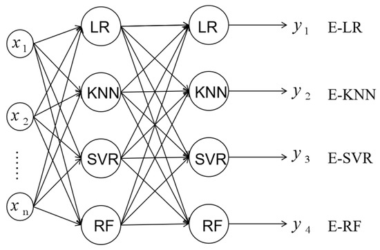
Figure 1.
The topology of stacking machine learning models.
2.7. Transfer Learning
Transfer learning [37] is a machine learning method in which a trained model is reused on another related task as a starting point.
Fine-tuning [38] is a popular method for realizing transfer learning. It belongs to the category of parameter-transfer learning. Transfer learning can be implemented using fine-tuning in two ways. In the first way, models obtained from the source domain are taken as pre-training models. The model of the pre-training model is frozen. A classification or regression network is added after pre-training models. Samples from the target domain are used to train the added network. The second way is to freeze part parameters of pre-training models and use samples from the target domain to train the unfrozen network parameters.
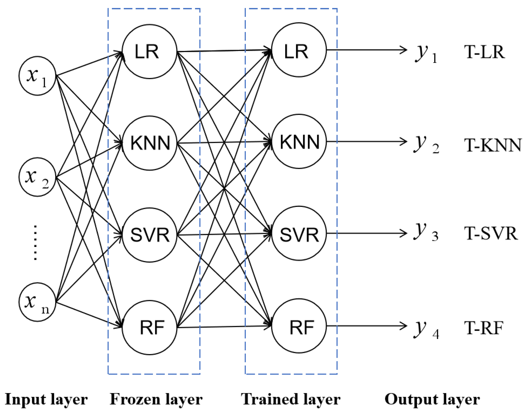
This research uses stacking ensemble learning models for predicting the Cr of container ships as the pre-training models for predicting 47,500 dwt bulk carrier resistance. In transfer learning, the first layer parameters are frozen, and the second layer parameters are trained using the bulk carrier data. According to the units in the second hidden layer, four transfer learning models are marked as transfer-LR (T-LR), transfer-KNN (T-KNN), transfer-SVR (T-SVR), and transfer-RF (T-RF), shown in Figure 2. represent the input features. represent the predicted Cr of T-LR, T-KNN, T-SVR, and T-RF, respectively.
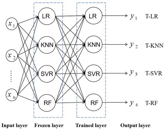
Figure 2.
The topology of transfer learning models.
2.8. Estimation Methods
Two estimation methods are used in this research as comparisons. One is the Holtrop and Mennen method, and another is the updated Guldhammer and Harvald method.
- (1)
- Holtrop and Mennen method (H-M)
J. Holtrop and G.G.J. Mennen developed the Holtrop and Mennen method for resistance and propulsion prediction based on the regression analysis of model tests and trial data of MARIN, the model basin in Wageningen, The Netherlands. In this method, the ship’s total resistance can be expressed using Equation (19).
where Rf is frictional resistance, 1 + k is the form factor, Rapp is appendage resistance, Rw is wave-making resistance, Rb is the resistance caused by the bulbous bow, Rtr is the resistance due to immersed transom, and Ra is the model ship correlation resistance.
Equation (19) is valid for:
Rapp and Rtr are ignored in this research. Therefore, the total resistance can be expressed using Equation (20).
Rf can be obtained using the ITTC-1957 equation. The sum of kRf, Rw, and Rb is called the residual resistance Rr, shown in Equation (21).
It is a flexible process to solve k, Rw, and Rb. The detailed process has been described by Holtrop [4].
- (2)
- The updated Guldhammer and Harvald method (updated G-H)
In 1965~1974, Guldhammer and Harvald developed an empirical method for ship resistance based on an extensive analysis of many published model tests. Harvald presents Cr as the curves of three parameters: the length-displacement ratio (), Cp, and Fn. Guldhammer proposed the regression equation in 1978 based on the analysis of Cr curves, shown in Equation (22).
Equation (22) is valid for .
Considering the impact of hull form, bulbous bow, and position of Lcb, Cr is corrected, as shown in Equation (23).
where the corrected resistance caused via Lcb is ignored.
In recent years, the shape of the bulbous bow has changed greatly. New Cr correction equations caused by the bulbous bow are proposed by Kristensen [11].
For tankers and bulk carriers, the Cr correction caused by the bulbous bow can be approximated using Equation (24).
Equation (24) is valid for , .
For container ships, the correction can be approximated using Equation (25).
Equation (25) is valid for .
2.9. Training Process
The training process of machine learning includes ship feature selection, data set division, model parameter tuning, and evaluation metrics.
- (1)
- Ship feature selection
In this research, Fn and the hull form parameters ∇/Lwl3, B/T, Cp, Cm, Cw, Lcb/Lwl, and Lcf/Lwl are taken as the input features of prediction models. Cr is taken as the prediction target. Ct can be obtained by summing Cr and Cf.
The distribution of Fn, ∇/Lwl3, B/T, Cp, Cm, Cw, Lcb/Lwl, Lcf/Lwl, and Cr is shown in Table 3, where the italicized numbers are values of the bulk carrier. It can be seen that the distribution of features is different between the bulk carrier and the container ships.
Table 3.
Distribution of samples. The italicized numbers are the bulk carrier values, and the upright numbers are the values of container ships.
- (2)
- Data preprocessed
The preprocessed data include standardization and normalization. Data normalization involves scaling the data to fit within a specific interval or distribution. It is commonly employed when processing indicators for comparisons and evaluations, removing unit limitations, and converting data into dimensionless values. The objective of normalization is to confine the preprocessed data within a defined range to mitigate the undesirable effects of individual sample data.
- (3)
- Data set division of container ships
In machine learning, a dataset is typically split into two distinct sets, the training set and the test set, based on a predetermined proportion. This study adopts the K-fold cross-validation method for dataset partitioning. The K-fold cross-validation approach divides the data into K mutually exclusive subsets, with each subset serving as the test set, while the remaining K-1 subsets are utilized as the training set to train the model. Subsequently, the outcomes of K models are aggregated using averaging or other techniques to determine the final model performance.
In ensemble learning, the dataset includes data from the 1100-TEU, 4250-TEU, 9000-TEU, and 13,500-TEU container ships designated as the training set. Meanwhile, the data from the 4700-TEU container ship and the KCS at the design draft serve as the test set, as illustrated in Figure 3. The training samples are partitioned into five subsets using the stratified sampling method. Each subset group is alternatively assigned as the validation set, with the remaining four subsets utilized for training. This division maintains a ratio of 4:1 between training and validation samples.
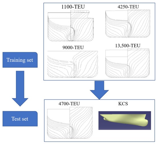
Figure 3.
Data division of container ships.
- (4)
- Data set division of the bulk carrier
The K-fold cross-validation method is employed in the dataset partitioning for the 47,500 dwt bulk carrier. Six draft states (5 m, 6.2 m, 7.5 m, 9 m, 10.2 m, and 10.7 m) are considered for the bulk carrier. Among these, the data corresponding to draft states of 5 m, 7.5 m, and 10.2 m are designated as the training set, while the remaining data are allocated to the test set. Validation samples are derived from the training set utilizing the stratified random sampling method, maintaining a ratio of 2:1 between training and validation samples.
It is worth noting that the number of test samples in this research is equal to that of training samples, aiming to investigate the prediction performance of transfer learning with a small training sample size.
- (5)
- Model parameters tuning
To achieve the best prediction performance, the parameters of the prediction models are tuned using evolutionary strategies in this research. The initial mutation strength of each model parameter is set to 2/3 of the search range, and the number of iterations is set to 200. The properties and search ranges of the parameters for the k-nearest neighbor (KNN), support vector regression (SVR), and random forest (RF) models are detailed in Table 4.
Table 4.
The parameter properties and search range of the KNN, SVR, and RF models.
- (6)
- Evaluation metrics
In this research, the maximum relative absolute error (Max-RAE) is employed for training prediction algorithms to mitigate the influence of the actual value on model training, as depicted in Equation (26). Both Max-RAE and the mean relative absolute error (Mean-RAE) are utilized to assess the accuracy of prediction results, expressed in Equations (27) and (28), respectively.
where ValueE represents the experimental value, ValueP represents the predicted value, and RAEi represents the RAE of the ith sample.
3. Results and Discussion
3.1. Prediction Results of Container Ships and Comparison
The Cr of a 4700-TEU container ship and KCS are predicted using basic ML models (LR, KNN, SVR, and RF), stacking ensemble learning models (E-LR, E-KNN, E-SVR, and E-RF), and estimation methods (H-M, updated G-H), respectively. The prediction results and errors of Ct of these two container ships using different methods are shown in Figure 4 and Figure 5 and Table 5.
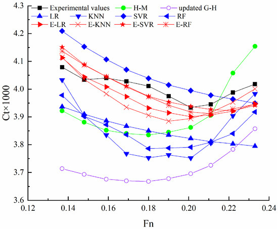
Figure 4.
The predicted Ct of 4700-TEU container ship using different methods.
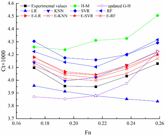
Figure 5.
The predicted Ct of KCS using different methods.
Table 5.
The prediction errors of Ct of 4700-TEU container ship and KCS using different methods.
3.2. Prediction Results of the Bulk Carrier and Comparison
Transfer learning is a machine learning method that leverages the ‘experience’ gained in one domain to a similar domain to address a problem. One of its advantages is that it requires only a small amount of data to fine-tune the model, leading to better learning outcomes and reduced dependence on the number of samples.
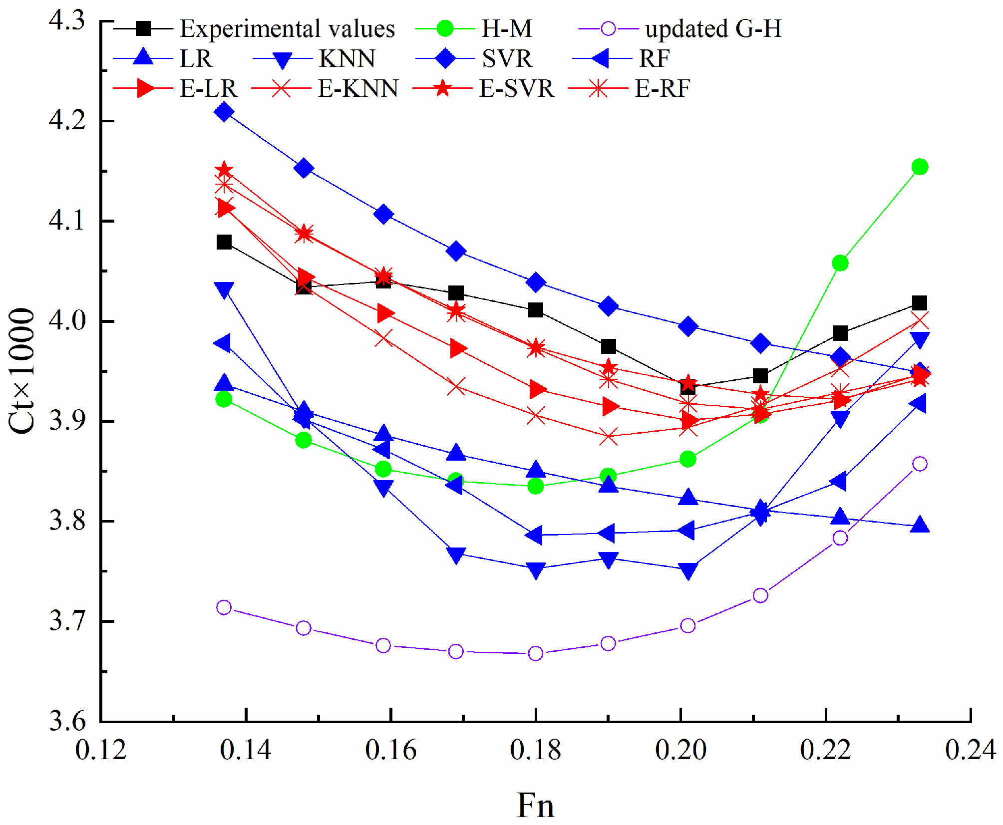
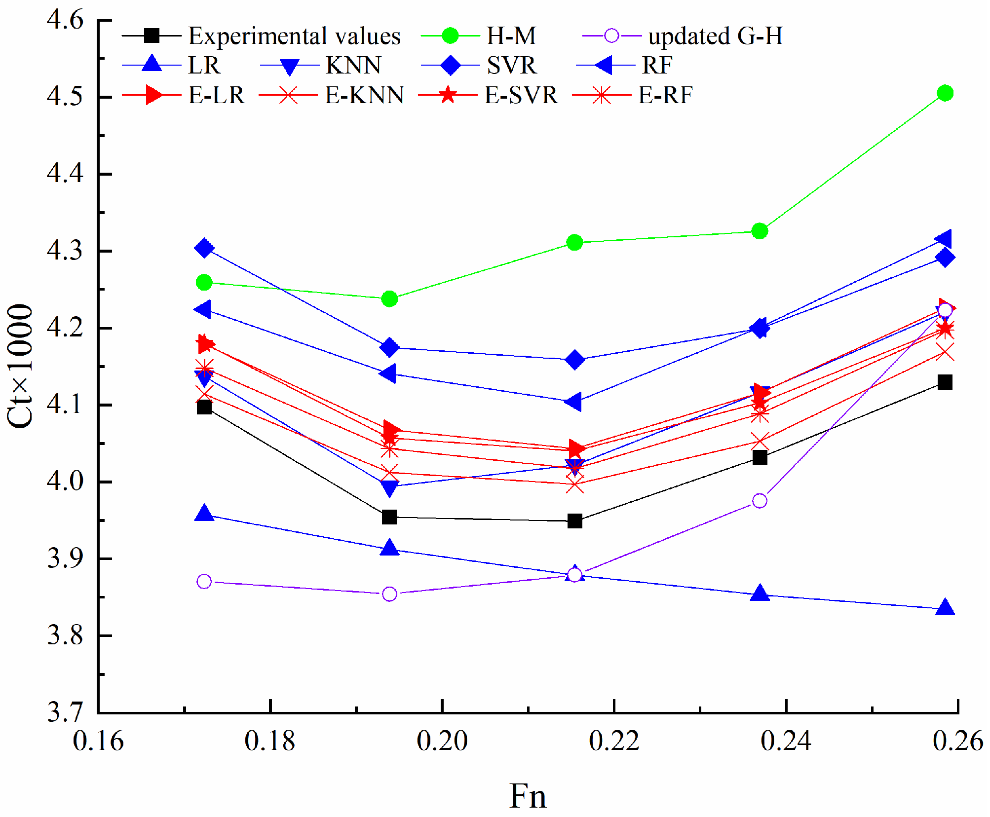
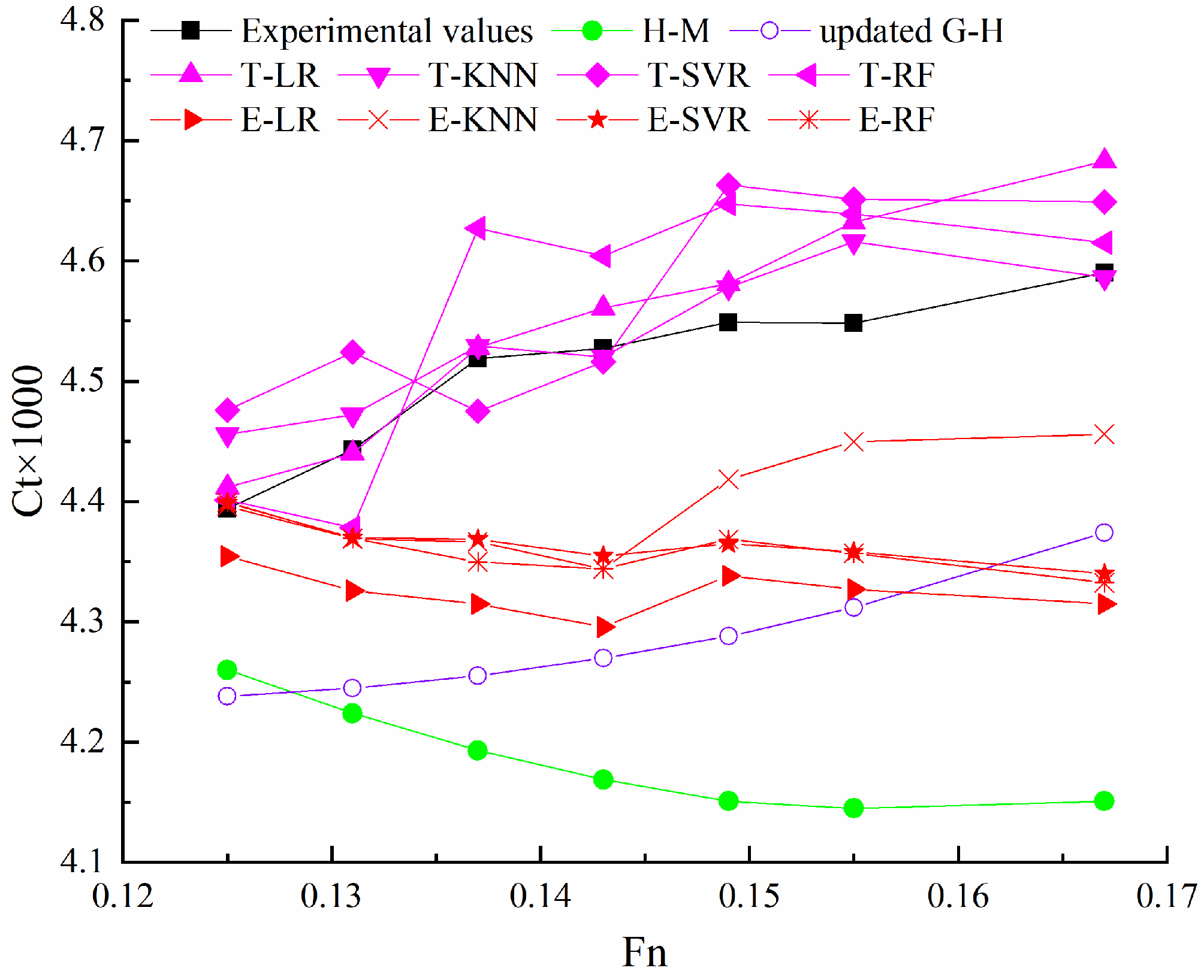
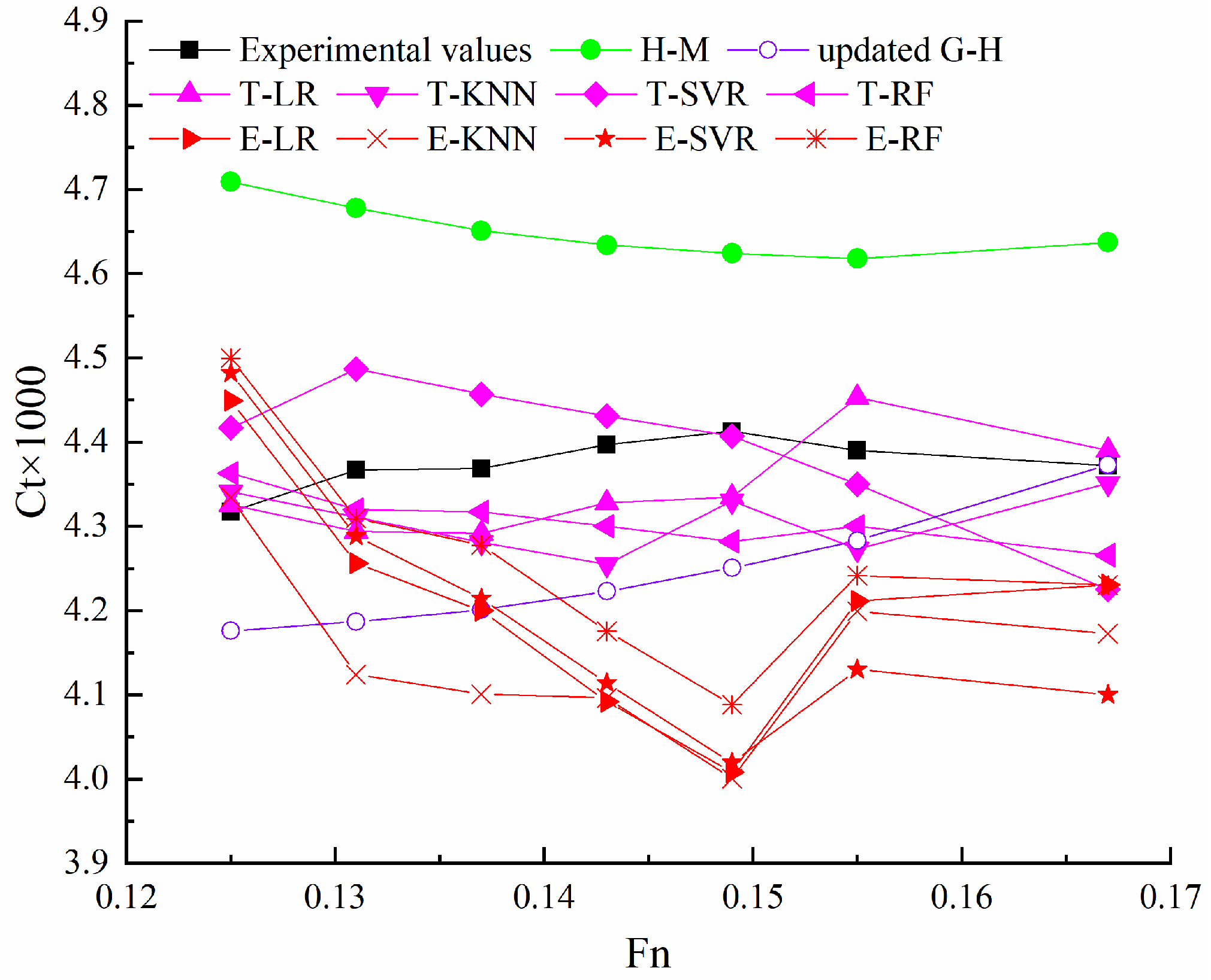
In this study, the Cr of the 47,500 dwt bulk carrier is predicted using stacking ensemble learning models (E-LR, E-KNN, E-SVR, and E-RF) trained on data from container ships, transfer learning models (T-LR, T-KNN, T-SVR, and T-RF), and estimation methods (H-M, updated G-H). The prediction results and errors associated with different methods are illustrated in Figure 6, Figure 7 and Figure 8 and summarized in Table 6.
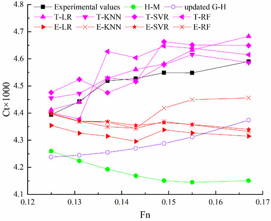
Figure 6.
The predicted Ct of the 47,500 dwt bulk carrier using different methods at Ts = 6.2 m.
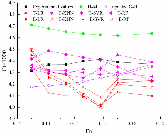
Figure 7.
The predicted Ct of the 47,500 dwt bulk carrier using different methods at Ts = 9 m.
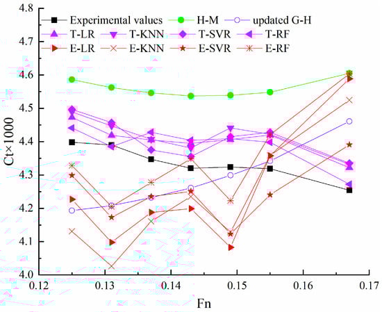
Figure 8.
The predicted Ct of the 47,500 dwt bulk carrier using different methods at Ts = 10.7 m.
Table 6.
The prediction errors of Ct of 47,500 dwt bulk carrier using different methods.
3.3. Discussion
The prediction results of container ships show that the prediction errors using stacking ensemble learning models are smaller than those using estimation methods. Moreover, compared with the corresponding basic ML models, the prediction accuracy of the ensemble learning model is enhanced. For instance, the prediction results of E-LR exhibit greater accuracy than those of LR. Notably, among the basic ML models, the model with the best performance corresponds to the ensemble learning model that exhibits the best performance among all ensemble learning models.
The ranges of Mean-RAE and Max-RAE using four stacking ensemble learning models of the 4700-TEU container ship are [0.919%, 1.257%] and [1.803%, 2.627%], and those of KCS are [0.915%, 2.337%] and [1.461%, 2.878%]. Prediction curves varied with Fn of all stacking ensemble learning models are similar and close to experimental values. In basic ML models, the ranges of prediction errors are larger compared to stacking ensemble learning models. The prediction curves of the KNN, the RF of the 4700-TEU container ship, and the KNN, SVR, and RF of KCS are also similar to those of experimental values. The prediction curves of LR used for the 4700-TEU container ship and KCS are similar. This is because the prediction results of LR are determined via all training samples. The prediction curves of SVR and LR of the 4700-TEU container ship are also similar, but the prediction results of SVR are mainly affected by local training samples. In the two estimation methods, the prediction results of the updated Guldhammer and Harvald method are smaller than those of H-M. The prediction curves of the two estimation methods are similar.
The ranges of Mean-RAE and Max-RAE using the four stacking ensemble learning models for the 4700-TEU container ship are [0.919%, 1.257%] and [1.803%, 2.627%], respectively, while for the KCS, they are [0.915%, 2.337%] and [1.461%, 2.878%]. It is observed that the prediction curves, varying with Fn, of all stacking ensemble learning models are similar and closely align with experimental values.
In contrast, the basic ML models exhibit larger ranges of prediction errors compared to the stacking ensemble learning models. Despite this, the prediction curves of certain basic ML models, such as KNN and RF for the 4700-TEU container ship and KNN, SVR, and RF for the KCS, are similar to the experimental values. The prediction curves of LR for both the 4700-TEU container ship and the KCS are also similar, as LR’s prediction results are determined using all training samples.
Interestingly, the prediction curves of SVR and LR for the 4700-TEU container ship are also similar, but SVR’s prediction results are primarily influenced by local training samples. Among the two estimation methods, the prediction results of the updated Guldhammer and Harvald method are smaller than those of the H-M method. Nevertheless, the prediction curves of both estimation methods are similar.
Based on the comparison of errors in resistance prediction for both the KCS and the 4700-TEU container ships among the four stacking ensemble learning models, E-KNN emerges as the recommended choice for predicting the resistance of container ships.
In the prediction results for the bulk carrier, transfer learning models exhibit higher prediction accuracy compared to stacking ensemble learning models and estimation methods. The prediction curves of transfer learning models show better alignment with experimental values across different Froude numbers. Conversely, the prediction curves of stacking ensemble learning models sometimes diverge from the experimental values, indicating that models trained on data from container ships may not be suitable for predicting the resistance of the bulk carrier. Additionally, the prediction curves of the two estimation methods, H-M and updated G-H, differ, making it challenging to determine the bulk carrier resistance using these methods accurately.
T-LR is recommended for predicting bulk carrier resistance based on the comparison of errors among the four transfer learning models.
The large errors observed in the H-M and updated G-H methods may be attributed to several factors. Firstly, these methods may have limitations due to their relatively older nature, suggesting potential for further refinement and improvement. Secondly, while these methods are commonly used for estimating ship resistance across various vessel types, their application may not be optimized for specific ship types, such as container ships and bulk carriers. Consequently, the errors in prediction may be more pronounced when applied outside their typical range of application. However, in cases of insufficient data samples, resorting to traditional empirical formulas remains an effective method for resistance forecasting.
The performance of stacking ensemble learning and transfer learning models indeed appears promising, and their structures share similarities. Both methods utilize a multi-layer network structure where the first layer network parameters are trained using data from container ships. However, their application and training processes differ.
In stacking ensemble learning, both training and test samples come from container ships. On the other hand, transfer learning involves training pre-existing models with container ship data and then fine-tuning them using data from a bulk carrier for re-training and testing.
The choice of input features significantly influences prediction accuracy. Stacking ensemble learning models employ a multi-layer network structure, where each layer learner aims to predict target values. This structure enhances the relationship between the prediction results of each basic learner and the target values, thus improving prediction accuracy.
4. Conclusions
In summary, the research on machine learning ship resistance prediction using stacking ensemble learning and transfer learning has yielded the following conclusions:
- Novel prediction methods: The proposed methods based on stacking ensemble learning and transfer learning offer efficient and accurate means of predicting ship resistance. These methods utilize ship data containing relevant parameters to evaluate resistance, which is particularly beneficial in the early stages of ship design;
- Improved accuracy for container ships: Stacking ensemble learning models outperform basic machine learning models and traditional estimation methods in predicting resistance for container ships. Among these models, E-KNN is recommended for the most accurate predictions;
- Transfer learning for bulk carriers: By leveraging pre-training with stacking ensemble learning models developed for container ships, transfer learning enables accurate prediction of bulk carrier resistance even with limited data. T-LR emerges as the preferred model for this prediction task.
These findings highlight the efficacy of machine learning techniques, particularly stacking ensemble learning and transfer learning, in ship resistance prediction across different ship types. They offer valuable insights for optimizing ship design processes and improving overall performance evaluation.
By leveraging machine learning techniques, such as stacking ensemble learning and transfer learning, the accuracy of resistance prediction has been substantially improved compared to traditional methods. The smaller error rates achieved using these novel approaches demonstrate their potential for enhancing the efficiency and effectiveness of ship design processes.
Moreover, the introduction of these advanced prediction methods opens up new avenues for research and development in the field of ship intelligence. Future studies can further refine and optimize ship resistance prediction models by incorporating cutting-edge machine learning algorithms, leading to even greater accuracy and efficiency in ship design and performance evaluation.
Overall, the findings presented in this study mark a significant contribution to the field of ship resistance prediction and lay the foundation for future advancements in ship intelligence and design optimization.
Author Contributions
Methodology, B.Z.; Software, Y.Y., Z.Z., J.Z. and Q.H.; Validation, Q.H.; Investigation, Y.Y. and L.Z.; Resources, J.S.; Data curation, Z.Z., J.Z., B.Z. and J.S.; Writing—original draft, Y.Y. and L.Z.; Writing—review & editing, Y.Y. and Z.Z.; Supervision, J.S. All authors have read and agreed to the published version of the manuscript.
Funding
The authors gratefully acknowledge the financial support from the National Natural Science Foundation of China (approval No. 12072126 and No. 51679097) and the Major Project for Special Technology Innovation of Hubei Province (Grant No. 2019AAA041).
Institutional Review Board Statement
Not applicable.
Informed Consent Statement
Not applicable.
Data Availability Statement
The data presented in this study are available upon request from the corresponding author due to privacy.
Conflicts of Interest
The authors declare that there are no known competing financial interests or personal relationships that could have appeared to influence the work reported in this paper.
References
- ITTC. Recommended procedures and guidelines 7.5-02-02-01, Resistance tests. In Proceedings of the International Towing Tank Conference, Virtual, 13–18 June 2021. [Google Scholar]
- Savisky, D. Hydrodynamic Design of Planing Hulls. Mar. Technol. 1964, 1, 71–95. [Google Scholar]
- Hollenbach, K.U. Estimating Resistance and Propulsion for Single-Screw and Twin-Screw Ships-Ship Technology Research. Schiffstechnik 1998, 45, 72. [Google Scholar]
- Holtrop, J. A Statistical Re-Analysis of Resistance and Propulsion Data. Int. Shipbuild. Prog. 1984, 31, 272–276. [Google Scholar]
- Calisal, S.M.; Dan, M.G. Resistance Study on a Systematic Series of Low L/B Vessels. Mar. Technol. 1993, 30, 286–296. [Google Scholar] [CrossRef]
- Robinson, J. Performance Prediction of Chine and Round Bilge Hull Forms. In Proceedings of the International Conference Hydrodynamics of High Speed Craft, London, UK, 24–25 November 1999. [Google Scholar]
- Lang, X.; Mao, W. A Semi-Empirical Model for Ship Speed Loss Prediction at Head Sea and its Validation by Full-Scale Measurements. Ocean Eng. 2020, 209, 107494. [Google Scholar] [CrossRef]
- Taskar, B.; Andersen, P. Benefit of Speed Reduction for Ships in Different Weather Conditions. Transp. Res. Part D Transp. Environ. 2020, 85, 102337. [Google Scholar] [CrossRef]
- Julianto, R.I.; Prabowo, A.R.; Muhayat, N.; Putranto, T.; Adiputra, R. Investigation of Hull Design to Quantify Resistance Criteria Using Holtrop’S Regression-Based Method and Savitsky’S Mathematical Model: A Study Case of Fishing Vessels. J. Eng. Sci. Technol. 2021, 16, 1426–1443. [Google Scholar]
- Gupta, P.; Taskar, B.; Steen, S.; Rasheed, A. Statistical Modeling of Ship’S Hydrodynamic Performance Indicator. Appl. Ocean Res. 2021, 111, 102623. [Google Scholar] [CrossRef]
- Kristensen, H.O.; Bingham, H. Prediction of Resistance and Propulsion Power of Ships. Technical Report of Technical University of Denmark. 2017. Available online: https://www.mek.dtu.dk/english/-/media/institutter/mekanik/sektioner/fvm/english/software/ship_emissions/wp-2-report-4-resistance-and-propulsion-power-final.pdf?la=da&hash=EC55C61EFB7434B32C91739E4F9D78046532F261 (accessed on 20 January 2024).
- Tu, H.; Yang, Y.; Zhang, L.; Xie, D.; Lyu, X.; Song, L.; Guan, Y.M.; Sun, J. A Modified Admiralty Coefficient for Estimating Power Curves in EEDI Calculations. Ocean Eng. 2018, 150, 309–317. [Google Scholar] [CrossRef]
- Crudu, L.; Bosoancă, R.; Obreja, D. A Comparative Review of the Resistance of a 37,000 Dwt Chemical Tanker Based on Experimental Tests and Calculations. Technium 2019, 1, 59–66. [Google Scholar] [CrossRef]
- Larsson, L.; Stern, F.; Visonneau, M. Numerical Ship Hydrodynamics: An Assessment of the Gothenburg 2010 Workshop; Springer: Berlin/Heidelberg, Germany, 2013. [Google Scholar]
- Kim, M.; Hizir, O.; Turan, O.; Day, S.; Incecik, A. Estimation of Added Resistance and Ship Speed Loss in a Seaway. Ocean Eng. 2017, 141, 465–476. [Google Scholar] [CrossRef]
- Lyu, X.; Tu, H.; Xie, D.; Sun, J. On Resistance Reduction of a Hull by Trim Optimization. Brodogr. Teor. I Praksa Brodogr. I Pomor. Teh. 2018, 69, 1–13. [Google Scholar] [CrossRef]
- Niklas, K.; Pruszko, H. Full-Scale CFD Simulations for the Determination of Ship Resistance as a Rational, Alternative Method to Towing Tank Experiments. Ocean Eng. 2019, 190, 106435. [Google Scholar] [CrossRef]
- Song, S.; Demirel, Y.K.; Atlar, M.; Dai, S.; Day, S.; Turan, O. Validation of the CFD Approach for Modelling Roughness Effect on Ship Resistance. Ocean Eng. 2020, 200, 107029. [Google Scholar] [CrossRef]
- ITTC. Recommended procedures and guidelines 7.5-03-02-03, Practical guidelines for ship CFD applications. In Proceedings of the International Towing Tank Conference, Virtual, 13–18 June 2021. [Google Scholar]
- Minh, N.V.; Thi, H.H.N.; Minh, N.P.; Van, T.D.; Huy, H.N.; Ngoc, T.T. Numerical Simulation Flow Around The 4600DWT Cargo Ship in Calm Water Condition Using RANSE Method. IOP Conf. Ser. Earth Environ. Sci. 2023, 1278, 012024. [Google Scholar]
- Roberto, R.; Soonseok, S.; Weichao, S.; Tonio, S.; Claire, D.M.M.-F.; Tahsin, T.; Kemal, D.Y. CFD analysis of the effect of heterogeneous hull roughness on ship resistance. Ocean Eng. 2022, 258, 111733. [Google Scholar]
- Margari, V.; Kanellopoulou, A.; Zaraphonitis, G. On the use of Artificial Neural Networks for the Calm Water Resistance Prediction of MARAD Systematic Series’ Hullforms. Ocean Eng. 2018, 165, 528–537. [Google Scholar] [CrossRef]
- Cepowski, T. The Prediction of Ship Added Resistance at the Preliminary Design Stage by the Use of an Artificial Neural Network. Ocean Eng. 2020, 195, 106657. [Google Scholar] [CrossRef]
- Yildiz, B. Prediction of residual resistance of a trimaran vessel by using an artificial neural network. Brodogradnja 2022, 73, 127–140. [Google Scholar] [CrossRef]
- Martić, I.; Degiuli, N.; Majetić, D.; Farkas, A. Artificial neural network model for the evaluation of added resistance of container ships in head waves. J. Mar. Sci. Eng. 2021, 9, 826. [Google Scholar] [CrossRef]
- Martić, I.; Degiuli, N.; Grlj, C.G. Prediction of Added Resistance of Container Ships in Regular Head Waves Using an Artificial Neural Network. J. Mar. Sci. Eng. 2023, 11, 1293. [Google Scholar] [CrossRef]
- Mentes, A.; Yetkin, M. An application of soft computing techniques to predict dynamic behaviour of mooring systems. Brodogradnja 2022, 73, 121–137. [Google Scholar] [CrossRef]
- Ozsari, I. Predicting main engine power and emissions for container, cargo, and tanker ships with artificial neural network analysis. Brodogradnja 2023, 74, 77–94. [Google Scholar] [CrossRef]
- Yang, Y.; Tu, H.; Song, L.; Chen, L.; Xie, D.; Sun, J. Research on Accurate Prediction of the Container Ship Resistance by RBFNN and Other Machine Learning Algorithms. J. Mar. Sci. Eng. 2021, 9, 376. [Google Scholar] [CrossRef]
- Elik, C.; Danman, D.B.; Khan, S.; Kaklis, P. A reduced order data-driven method for resistance prediction and shape optimization of hull vane. Ocean Eng. 2021, 235, 109406. [Google Scholar]
- Hino, T.; Stern, F.; Larsson, L.; Visonneau, M.; Hirata, N.; Kim, J. Numerical Ship Hydrodynamics: An Assessment of the Tokyo 2015 Workshop; Springer Nature: Berlin, Germany, 2020. [Google Scholar]
- Seal, H.L. Studies in the History of Probability and Statistics. XV the Historical Development of the Gauss Linear Model. Biometrika 1967, 54, 1–24. [Google Scholar] [PubMed]
- Yan, X.; Su, X. Linear Regression Analysis: Theory and Computing; World Scientific: Singapore, 2009. [Google Scholar]
- Altman, N.S. An Introduction to Kernel and Nearest-Neighbor Nonparametric Regression. Am. Stat. 1992, 46, 175–185. [Google Scholar] [CrossRef]
- Breiman, L. Random Forests. Mach. Learn. 2001, 45, 5–32. [Google Scholar] [CrossRef]
- Zhou, Z.; Chen, S.F. Neural Network Ensemble. Chin. J. Comput. Chin. 2002, 25, 1–8. [Google Scholar]
- Torrey, L.; Shavlik, J. Transfer Learning, Handbook of Research on Machine Learning Applications and Trends: Algorithms, Methods, and Techniques; IGI Global: Hershey, PA, USA, 2010; pp. 242–264. [Google Scholar]
- Tajbakhsh, N.; Shin, J.Y.; Gurudu, S.R.; Hurst, R.T.; Kendall, C.B.; Gotway, M.B.; Liang, J. Convolutional Neural Networks for Medical Image Analysis: Full Training or Fine Tuning? IEEE Trans. Med. Imaging 2016, 35, 1299–1312. [Google Scholar] [CrossRef]


Disclaimer/Publisher’s Note: The statements, opinions and data contained in all publications are solely those of the individual author(s) and contributor(s) and not of MDPI and/or the editor(s). MDPI and/or the editor(s) disclaim responsibility for any injury to people or property resulting from any ideas, methods, instructions or products referred to in the content. |
© 2024 by the authors. Licensee MDPI, Basel, Switzerland. This article is an open access article distributed under the terms and conditions of the Creative Commons Attribution (CC BY) license (https://creativecommons.org/licenses/by/4.0/).