Article

Coupled Inversion of Amplitudes and Traveltimes of Primaries and Multiples for Monochannel Seismic Surveys

National Institute of Oceanography and Applied Geophysics—OGS, 34010 Sgonico, Italy
*
Author to whom correspondence should be addressed.
J. Mar. Sci. Eng. 2024, 12(4), 588; https://doi.org/10.3390/jmse12040588
Submission received: 20 February 2024 / Revised: 18 March 2024 / Accepted: 28 March 2024 / Published: 29 March 2024
(This article belongs to the Section Coastal Engineering)

Abstract

:
Engineers need to know properties of shallow marine sediments to build piers, pipelines and even offshore windfarms. We present a method for estimating the density, P velocity and thickness of these sediments. The traveltime inversion of primary and multiple reflections enables their semiquantitative estimation in marine surveys when using a minimal acquisition system such as a monochannel Boomer. Picking errors, ambient noise and interfering events lead to significant errors in the estimates. Similar, albeit milder, instabilities occur when inverting the signal amplitudes to determine the reflectivity of the layer interfaces. In this paper, we introduce a coupling between the separate inversion of amplitudes and traveltimes to obtain a better Earth model. The P velocity shows up in two stable terms provided by the separate inversions: the acoustic impedance of shallow sediments (through the amplitudes) and the transit time across the sediment layer (through the traveltimes). We couple the two inversion engines by imposing a smoothness condition on velocity and density and thickness of the layer while keeping the impedance and traveltime constant. We thus exploit the ambiguity of the solution to introduce geological criteria and reduce the noise contribution. We validated the proposed method with synthetic and real data.

1. Introduction

Offshore engineering and environmental studies require precise knowledge of the lithological properties of shallow marine sediments. Multi-channel seismic profiling or, even better, using ocean-bottom cables [1] can provide high-resolution images over wide areas [2,3]; however, the associated costs can only be borne for large-scale projects such as the construction of platforms for oil and gas exploration [4] or large wind farms [5,6,7,8]. For smaller engineering projects in high-traffic areas such as harbors [9], archeological areas [10] or sensitive environments [11,12,13], the low cost and ease of use of Boomer surveys may be the only viable option [14,15,16,17,18,19,20]. For monochannel systems, the estimation of rock parameters such as P velocity, density and thickness of shallow marine sediments becomes a challenge. However, these parameters are needed by offshore engineers for pipeline and jetty design [21,22] and by marine geologists to assess recent depositional conditions [23,24,25].
In multi-channel surveys, the layer velocity is determined by exploiting the traveltime difference between different offsets between source and receivers [26,27,28,29] and many others. When only one channel is available, tomographic inversion of traveltimes of primaries and multiples [30,31,32] provides a good estimate of velocity and thickness for noise-free synthetic data, but becomes unstable as the noise level increases. Better stability is achieved when the amplitudes of the seawater reverberation are inverted [33], probably because the associated signal is strong and easy to interpret. The amplitude inversion provides a robust estimate of the seabed reflectivity and indirectly the acoustic impedance of the shallow sediments [34]. P impedance, a product of density and P velocity, contains information about two important lithological parameters that we are looking for, but they cannot be unambiguously determined. A similar ambiguity exists with traveltime inversion, where the ratio between velocity and thickness is quite well determined, but not so much the two separate terms. As a result, we have two good pieces of information, but three unknowns to solve. In this paper, we introduce a coupling between the solutions obtained by amplitude and traveltime inversion. The “third constraint” required to turn our problem into a well-posed one is a smoothness condition for the many possible solutions that fit our data equally well. We can take advantage of the information redundancy resulting from the small spatial sampling, the size of which is smaller than the Fresnel zone. Moreover, the facies variations of marine sediments are mostly smooth, and we can force the inversion algorithm to embed our geological “a priori” information.
In recent papers, we presented the use of multiple reflections in monochannel Boomer surveys to determine the P velocity and acoustic impedance of shallow sediments from the traveltimes and amplitude of seismic signals, respectively (see below). However, both methods suffer from instabilities when the noise is significant and the distance between source and receiver is less than 5 m. In this paper, we show that linking the two inversion results can significantly improve their stability and reliability if a shared Earth model and smoothness principle are used.

2. Materials and Methods

2.1. Inversion Strategy

Figure 1 shows the most important parameters of our assumed 1D Earth model, which consists of seawater and a layer of sediments overlying a half-space. The density r0 and the P velocity V0 of the seawater are assumed to be known, as is the offset x between source and receiver. The parameters to be inverted are the water depth Wd, and three parameters for the sediment layer: thickness Lt, P velocity V1 and density r1.
We note that the reliability of the inversion is very unbalanced for these unknowns. The water depth is very accurate, while there is a significant cross talk between thickness and velocity of the sediment layer and the density is even less stable. The latter can be determined indirectly by inverting the amplitude of the reverberations in the seawater layer [33], which provides a good estimate for the reflectivity R1 of the seabed. As the acoustic impedance of the seawater r0 V0 is known, we can calculate the acoustic impedance I1 of the shallow sediments using the following formula:
I 1 = r 1   V 1 = r 0   V 0   1 + R 1 1 R 1
We must first estimate the sediment velocity V1 in order to calculate the density r1 by the simple ratio:
r1 = I1/V1
A fair estimate of the sediment velocity can be obtained by the joint traveltime inversion of direct arrivals and primary and multiple reflections [30,31].
Figure 2 shows the main multiples that can be used, i.e., peg leg, intrabed, and “simple”. At least one of them is needed in addition to the primary reflections. The robustness of the inversion can be improved by also including the water bottom reverberations.

2.2. Modeling Amplitudes and Traveltimes

The amplitudes of seismic signals propagating in the 1D Earth model in Figure 1 can be easily modeled by assuming straight ray paths for the seismic signals. The reflectivity R0 for the interface between air and sea surface under normal conditions is about 0.999438 and can be approximated by 1. The transmission coefficients T1_down and T1_up in the downward and upward directions at the seabed are [34]:
T1_down = 1 − R1,  T1up = 1 + R1
The amplitudes of the multiples can be calculated using the following equations:
Apegleg = −T1_down R2 T1_up R0 R1
Aintrabed = −T1_down R2 R1 R2 T1_up = −T1_down R1 R22 T1_up
Asimple = −T1_down R2 T1_up R0 T1_down R2 T1_up = −R0 (T1_down R2)2
Arever1 = −R1R0R1 = −R0 R12
Arever2 = R1R0R1R0R1 = R02 R13
where the variable names on the left are self-explanatory and correspond to the ray paths in Figure 1 in the same order. Note that the amplitude of the reverberations (4d) and (4e) depends only on the reflectivity of the sea surface and seabed, involving the properties of the seawater and sediment layer. These signals are normally strong and easy to interpret, so their inversion is reliable. However, when using Equations (4a)–(4c), the additional term R2 is added, i.e., the reflectivity of the sediment bottom, which is usually much weaker. For this reason, inversion for these first three amplitudes is a challenge, unless our data are virtually noise-free. The primary reflections from the seafloor and the sediment bottom provide further equations:
Aseafloor = R1
Asediment = T1_down R1 T1_up
A similar set of equations is available for the traveltimes, using the proper incidence angles ai for each multiple type and b for the primary reflection from the seafloor (Figure 3):
Tpegleg = 2 (2 Wd/V0 + Lt/V1)/cos a1,  a1 = atan (X/(4 Wd + 2 Lt))
Tintrabed = 2 (Wd/V0 + 2 Lt/V1)/cos a2,   a2 = atan (X/(2 Wd + 4 Lt))
Tsimple = 4 (Wd/V0 + Lt/V1)/cos a3,  a3 = atan (X/(4 Wd + 4 Lt))
Trever1 = 4 [Wd2 + (X/4)2]1/2/V1,
Trever2 = 6 [Wd2 + (X/6)2]1/2/V1,
Tseafloor = 2 [Wd2 + (X/2)2]1/2/V1,
Tsediment = 2 (Wd/V0 + Lt/V1)/cos b,   b = atan (X/(2 Wd + 2 Lt))
We note that almost all relations in (4) and (5) are highly nonlinear, so we cannot be surprised if their inversion to determine P velocity, density and thickness of sediments becomes unstable when the data are contaminated by noise. We will see in the coming sections that this drawback can be mitigated to some extent.

2.3. Inverting Amplitudes and Traveltimes

A classical approach for traveltime inversion, which we have also implemented, is the minimization of an object function ObTime(Tj, V, L), which is the sum of the squared differences between measured and simulated traveltimes, as a function of the trial velocities V and the thickness L:
ObTime ( T j ,   V ,   L ) = j [ T j t V ,   L ] 2 ,
where the summation index j runs over the available times Tj that were measured at a particular shot, ideally all from (5a) to (5g). The more terms available, the higher the redundancy of information, which is usually a good tool to reduce random noise. This minimization can be performed using a variety of mathematical tools, such as the conjugate gradient method or even exhaustive search, since the computational cost for each shot is low.
In principle, we could define a comparable object function ObAmpli(Aj, V, r) to invert for the layer velocity and density. We can replace the layer thickness L by its density r, and the time Equations (5a)–(5g) by the amplitude Equations (4a)–(4g):
ObAmpli ( A j ,   V ,   r ) = j [ A j a V , ρ ] 2 ,
Although this approach is mathematically feasible, it proves to be a weak one. The reason for this becomes clear when one considers a subset of Equations (5), i.e., (4d)–(4f). Since R0 is well approximated by 1, the amplitude moduli of the seafloor primary and its reverberations are R1, R12 and R13. As values for R1 commonly found experimentally are about 0.1, the contributions of the corresponding terms to the object function (6) comprise three different orders of magnitude. Therefore, the errors in the first may overwhelm the contribution of the second term and the second term that of the third term. If the R2 term also comes into play, we also include third- and fourth-order terms in the inversion algorithm. We need a different object function.
A possible better option results from normalizing the differences in (7) by the trial amplitude a(V, r):
ObANorm ( A j ,   V ,   r ) = j A j a V , ρ a V , ρ 2 .
In this way, all terms in the summation are of approximately the same order of magnitude and thus contribute to noise reduction in a balanced way.

2.4. Algorithm Details

The traveltime inversion of monochannel Boomer data can estimate the velocity and depth of seawater based on direct and reflected arrivals. However, the main target of high-resolution marine surveys for offshore engineering is the properties of shallow sediments such as thickness and P velocity. Their inversion becomes unstable when the offset between source and receiver is only a few meters [30,31]. Reducing this instability is a challenge. Some help can be provided by the ratio LV1 between the thickness L1 and the velocity V1 of the layer, which remains quite stable even in the presence of noise:
LV1 = L1/V1.
This ratio is the one-way traveltime for a seismic signal propagating vertically across the sediment layer. Thus, having a physical and geological meaning, we expect good lateral continuity along the profile, as the facies of shallow sediments usually changes only slowly. Another option is to introduce hard constraints in the form of upper and lower limits for the allowable velocity and thickness, but given the wide range of reasonable values found in actual surveys, this choice is a weak one.
If the tomographic inversion is not well constrained by the data and a null space exists (e.g., [35,36]), an infinite number of solutions may fit the data equally well. Among these solutions, we can choose one that satisfies geological criteria, ties to the wells, or is the interpreter’s use. A smooth variation seems to us to be most suitable for Boomer surveys, since these usually have a high spatial sampling, e.g., shot intervals of about 0.6 m. For a frequency of 3000 Hz for the source signal, a water depth of 20 m and a seawater velocity of 1500 m/s, the extension of the first Fresnel zone at the seafloor is 2.2 m [36,37]. This means that the lateral resolution of the illuminated area corresponds approximately to this size, so that we can hardly recognize finer details in our Earth images. Furthermore, since the shot interval is 0.6 m, almost 4 adjacent traces cover the same Fresnel zone, so a certain lateral smoothing of these traces at least is consistent with physical propagation.
Amplitude inversion of primaries and multiples similarly yields both weak and robust estimates. Inverting the reverberations between the sea surface and the sea floor [32] gives a stable result for the acoustic impedance I1 of the interface between seawater and shallow sediments:
I1 = r1 V1,
where r1 and V1 are the density and the P velocity of the sediments. The velocity V1 appears in both (9) and (10), the left-hand term of which can be taken as a good approximation for the unknown actual Earth parameters. If we keep these two terms as known constants, these relations become a system of two equations with the three unknowns L1, r1 and V1. This system of equations is clearly underdetermined.
Among the infinite solutions that satisfy both (9) and (10), we can select the one that satisfies an additional condition, namely, smoothness. We can limit or remove the isolated outliers by applying a smoothing filter S[*, n] along the profile to these unknowns:
L1′ = S[L1, n], V1 = S[V1, n],  r1 = S[r1, n],
where n is the filter length in samples. We can use a median filter, which removes possible spikes, but leaves the sharp discontinuities, or a Savitzky–Golay filter [38,39], which better preserves the high frequencies, but blurs the anomalies. Of course, the new smoother items usually do not satisfy Equations (9) and (10), thus violating reliable information we have obtained from amplitude and traveltime inversions. We can force the value LV1 in (9) to remain constant by computing a power p such that:
LV1 = (L1′/V1′)p.
Taking the natural logarithm of both sides of (12), we get:
ln[LV1] = ln[(L1′/V1′)p] = p ln[L1′/V1′],
which can be solved for p, obtaining:
p = ln[LV1]/ln[L1′/V1′].
Applying this power to L1′ and V1′, we get the smoothed, normalized values L1” and V1”:
L1” = (L1′)p,  V1” = (V1′)p,
which completely fulfil the condition (9). Similarly, if we constrain velocity and density by the acoustic impedance (10), we obtain a power q by imposing:
I1 = (r1′ V1′)q,
and obtaining:
q = ln[I1]/ln[r 1′ V1′].
Consequently, the normalized values are:
r1” = (r 1′)q,  V1” = (V1′)q.
The standard workflow starts with the traveltime inversion, where the velocity V1 is given in (10) to obtain the density r1. The improved value V1” provided by the normalization (18) may be used instead to accelerate the convergence to a smoother solution.
Figure 4 provides a visual feeling of the ambiguities we are addressing. In the 3D space of possible solutions for our parameters of the sediment layer, i.e., thickness, velocity and density, the constraints provided by (9) and (10) correspond to the red and blue surfaces, respectively. Their intersection is a line, highlighted by black dots, which still includes infinite solutions, but in 1D only. We can select one of them by choosing a smoothness criterion and parameter, such as the window length of a median or Savitzky–Golay filter. The conditioning by (18) imposes that the smoothed solutions are still located along the dotted line.

3. Application to Synthetic and Real Data

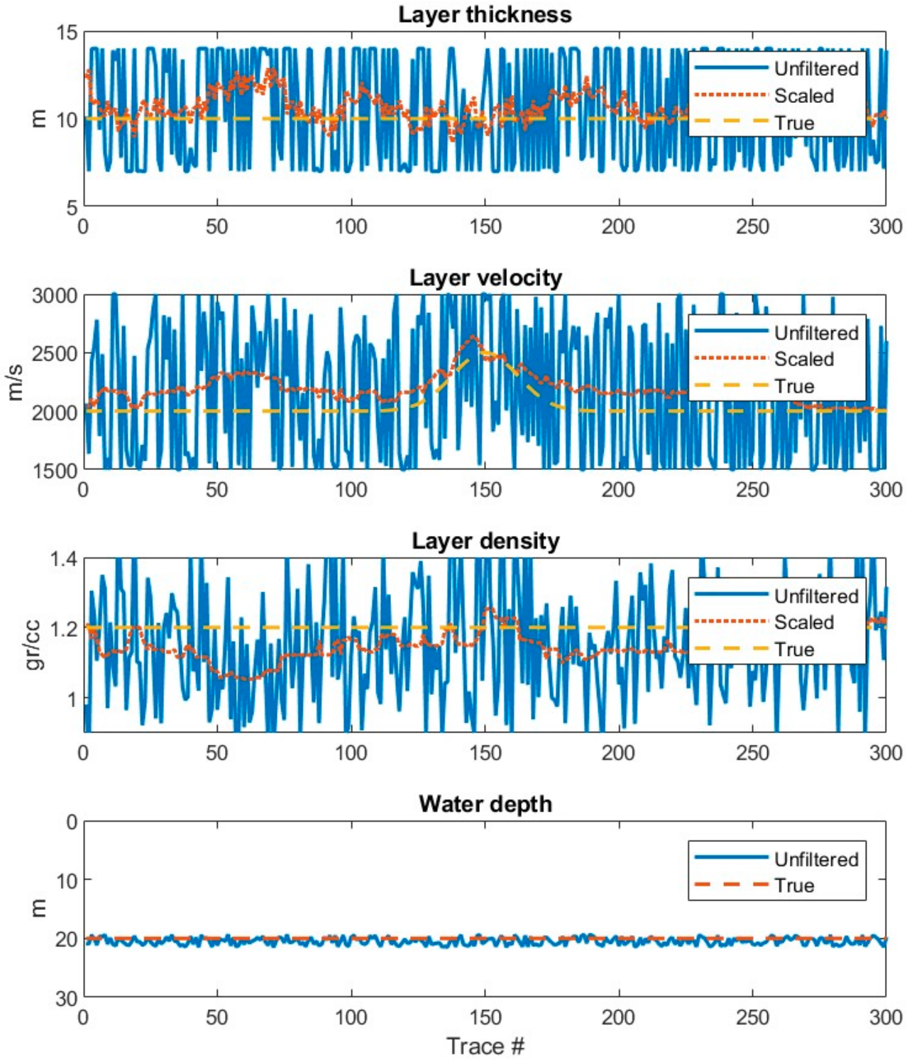
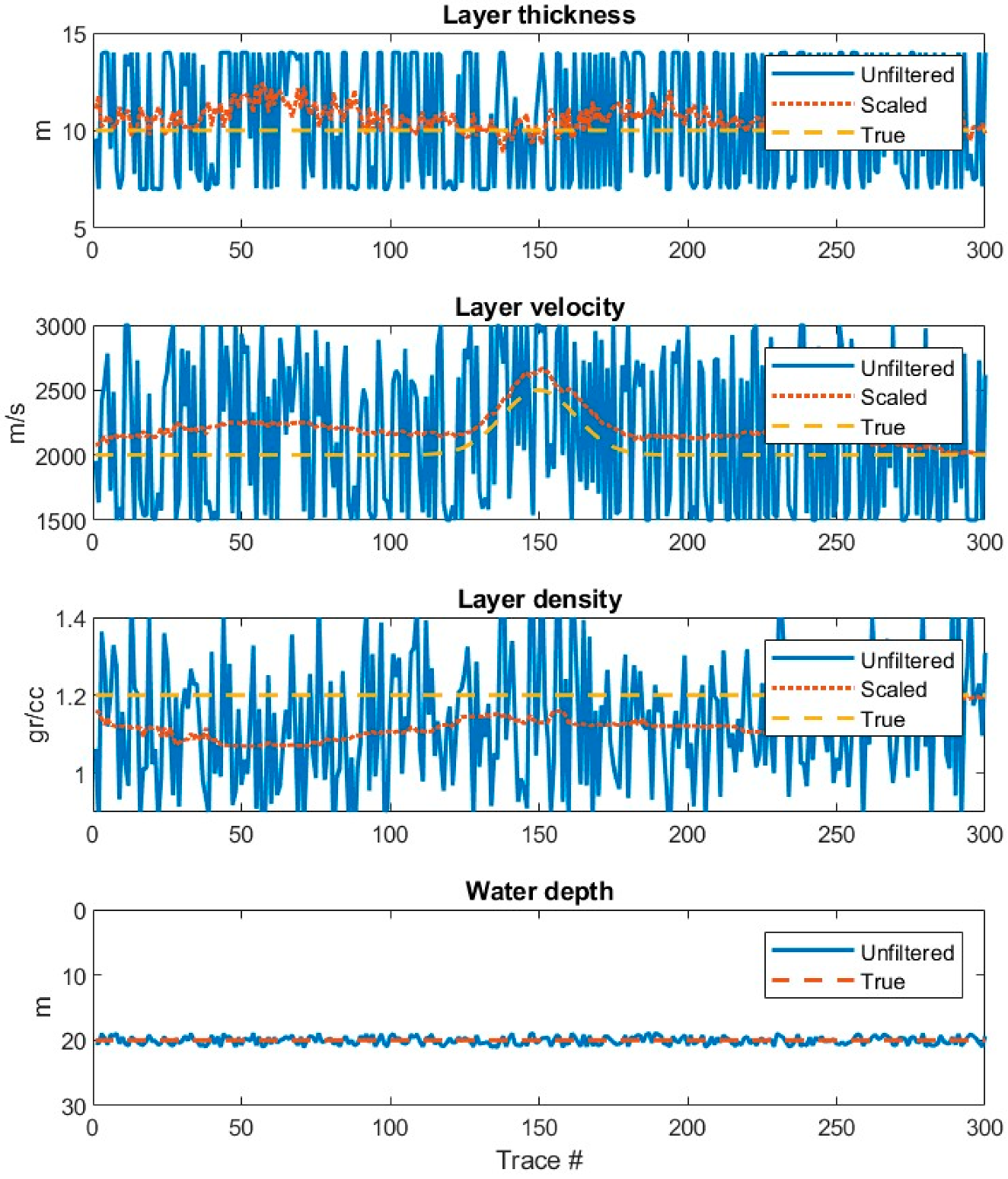
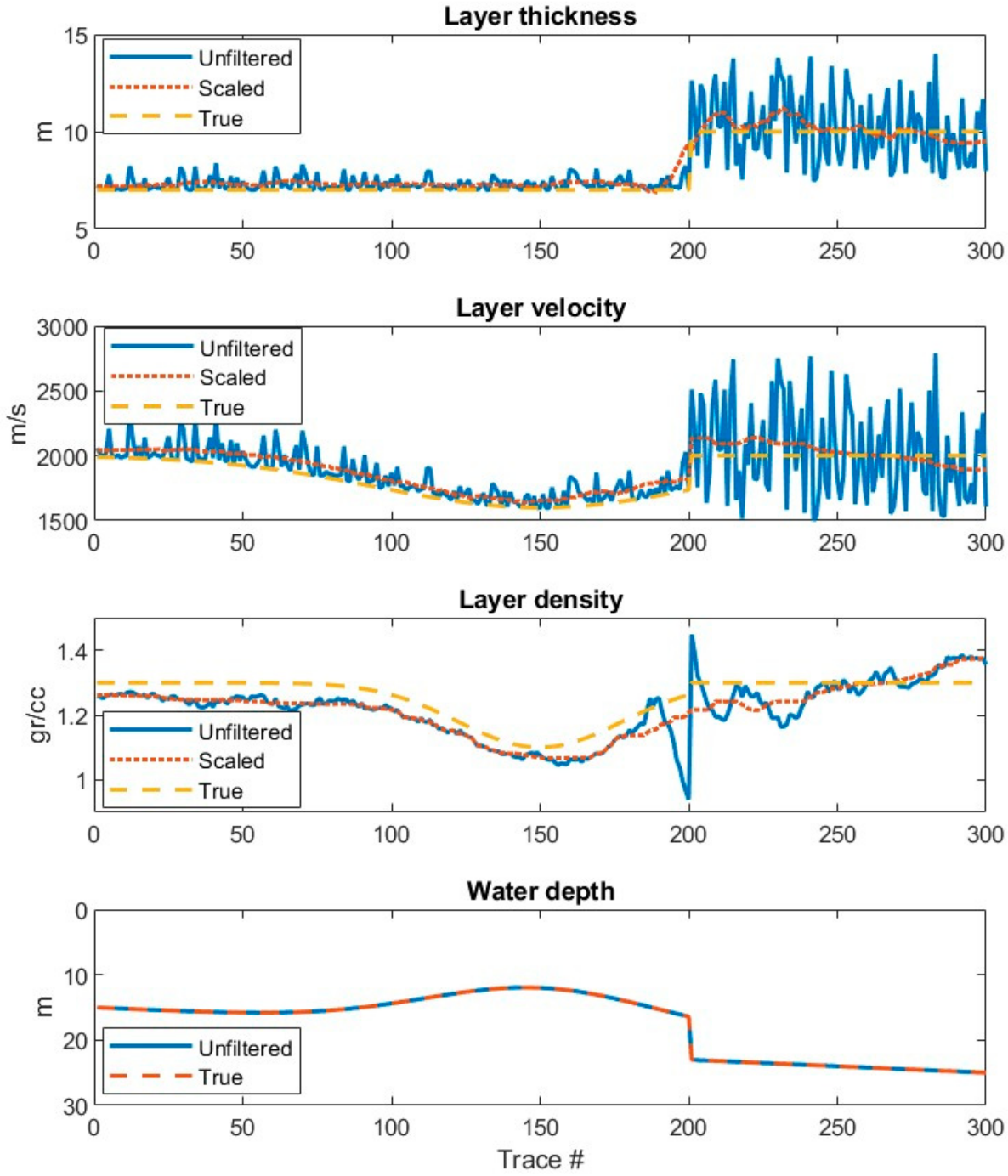
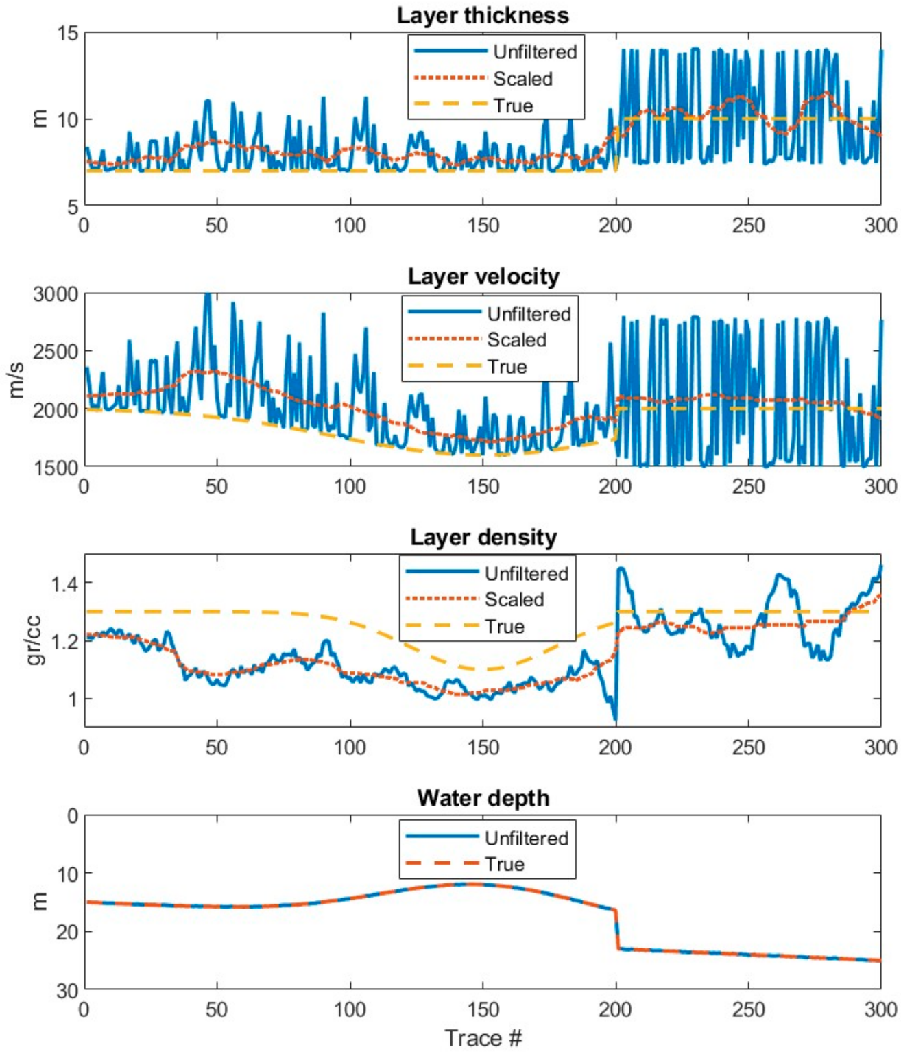
3.1. Validation by Synthetic Data

Figure 5 shows a simple 1D model with horizontal interfaces and a sediment layer with a smooth high-velocity anomaly in the central part (see also Table 1). The P velocity of the seawater and basement are constant, as is the density for all layers. With this model, we can evaluate the detectability of lateral velocity variations in the sediments with different noise levels.
We simulated a Boomer survey composed of 300 traces with an offset of 4.5 m between source and receiver. We calculated the amplitudes and traveltimes according to Equations (4) and (5) and perturbed them with random errors in the range of ±1%. The traveltimes range from about 7 ms for the direct arrivals to over 70 ms for the simple multiples, with most values around 40 ms; thus, an average maximum error of 400 µs was introduced. These errors are substantial, as typical sampling intervals are between 20 and 40 µs, corresponding to 10–20 samples in the misspeaks. Despite this noise, we obtained a fair estimate for the thickness, velocity and density of the sediment layer (Figure 6 and Figure 7). The solid blue line in all plots shows the estimates obtained by applying the simple inversion of Equations (4) and (5). Its oscillations are very large, and minor ripples show up even in the most stable estimate, i.e., the water depth. However, if the smoothing and scaling filter defined above is applied (dotted red line), the estimates stabilize considerably for a window length of 31 samples (Figure 6) or a longer one of 71 samples (Figure 7). The latter method in particular approximates the central velocity anomaly and a certain flatness of the layer thickness and density quite well.
Figure 8 shows a second, more complex model that includes both smooth and sharp discontinuities in the sediment parameters, i.e., thickness, P velocity and density. Table 2 summarizes its main parameters.
A central low-velocity anomaly mimics gas accumulation due to vertical leakage through a normal fault on the right side, where a thicker and dipping homogeneous block is located. The seawater and basement properties are the same as in the previous model, but the water depth changes significantly along the profile. We note that, strictly speaking, this model cannot be defined as a 1D model because of these lateral variations; however, we simulated each trace independently, assuming a local 1D model with the value of the vertical section at that trace position, and used the same approach in the following inversion. As a result, we do not consider diffraction or lateral events in our ray tracing, which is strictly 1D. Although the image is laterally compressed for visual convenience, this model is reasonable when these variations are diluted over long distances.
Figure 9 and Figure 10 show the results of the inversion when the data are affected by errors of 0.1% and 0.3%, respectively. These errors refer to one or very few samples, thus implying very accurate picking and a good signal-to-noise ratio of the data. The estimated lithological parameters are quite good in Figure 9 and just acceptable in Figure 10, indicating that the data quality is limited to achieve a good result. Both figures show large instabilities on the right-hand side in the estimated layer velocity and thickness before the smoothing filter (solid blue line). This is probably due to the greater water depth in this zone and the resulting larger percentage errors in the data. In both figures, a prominent double oscillation can be seen at the fault location, which is effectively removed by the lateral filtering.
Figure 11 compares simple smoothing operators with the scaling defined by (16) and (17). We calculated the LV1 value defined by (8), i.e., the vertical one-way traveltime across the sediment layer. On the left side, smoothing (solid blue line) using a Savitzky–Golay filter gives a nice line fitting the true model (yellow dashed line) well, except at the fault. The scaled curve (dotted red line) contains many small ripples, but performs much better at the fault. Comparable results are obtained with the median filter on the right. The main difference is the staircase-like appearance of the curve “smoothed” with the median filter (solid blue line), which—in contrast to the scaled curve (dotted red line)—does not define the correct fault position. All operators have the same length of 31 samples.

3.2. Application to Real Data

To validate our method with real data, we acquired a Boomer profile at the Santa Croce Lake in the Eastern Alps (Italy). It is a natural lake in the Piave Valley, which was extended by a dam in 1930. An overview of its geological setting is provided by [40]. We selected 400 traces in a profile where we could interpret the events necessary for our inversion algorithm: the primary reflections from the seafloor and the base of the sediments, the first and second reverberation in the water layer and the peg-leg multiple of the sediments. The source is a Boomer model AA301 (Applied Acoustic Engineering) with a frequency band in the range of 400–6000 Hz. The offset is approximately 4.5 m and the shooting interval approximately 0.7 m. For the seawater, we assume a standard value of 1500 m/s for the P velocity and a density of 1 g/cc, as these measurements were not carried out during the survey.
Figure 12 displays the Boomer profile after pure bandpass filtering to remove low-frequency noise due to spurious currents. Since no geometrical spreading has yet been applied, several diffraction hyperbolas due to plumes are clearly visible in the water layer between 0 and 50 ms. The seafloor is flat in the central part, while the base of the sediments (at about 75 ms) is slightly curved: this difference allows a better distinction between primaries and multiples. Other primary effects and diffractions are also visible in the deeper part.
Figure 13 shows the seismic section after correcting the spherical divergence only for propagation in seawater by multiplying each sample by the function Vw t, i.e., the velocity of the seawater and the sample traveltime [41]. Since we only invert the amplitudes of the reverberations in the water layer, we do not consider propagation effects, such as anelastic absorption in the sediments, which are appropriate when multiples across them are included. We picked both the amplitudes and traveltimes of the tracked horizons. The seafloor (red line) and its first and second multiple (green and blue lines, respectively) are clearly visible. We interpreted and picked the primary reflection from the sediment base (yellow line) and its peg-leg multiple (pink line), i.e., the primary reflection from the sediment base followed by a single bounce in the water layer.
The results of the inversion (Figure 14) show slight lateral fluctuations. The layer thickness and water depth are almost flat, while velocity and density fluctuate slightly in opposite directions. The velocity of the sediments is about 2000 m/s, while their density is approximately the same as that of the water. This low value is probably due to saturating fluids emerging from the seabed and moving upwards in the plumes, as can be clearly seen in Figure 12. The density is indeed lower between trace numbers 200 and 300, where we observe an increase in reflectivity at and just below the seafloor (Figure 12 and Figure 13). Such a phenomenon is often due to saturating fluids, so this fact could also explain our observations. The sediment velocity increases slightly in the same trace interval. This could be due to a stiffening of the rock matrix as a result of tectonic compression and uplift, which is clearly visible in all our sections.
The smoothing filter (dashed orange line in Figure 14) slightly improves the estimate of density, which is usually the most unstable element that is inverted. We used a filter length of 21 elements.

4. Discussion

In principle, a different strategy can be defined for the joint inversion of amplitudes and traveltimes, i.e., building a single object function ObAll containing all data and model parameters. For example, we could simply add the two object Functions (6) and (7):
ObAll ( A j ,   T j ,   V ,   L ,   r )   =   ObTime ( T j ,   V ,   L )   +   ObAmpli ( A j ,   V ,   r )   =   = j [ T j t V ,   L ] 2 + j [ A j a V , ρ ] 2 ,
or a normalized version of it, similar to (8). However, this would not take advantage of the different sensitivity of the data to noise or different inversion stability, thus not turning it to our advantage. The system of Equation (5) gives a stable result for the seawater depth and for the LV1 time in (9), while it is unstable when we try to determine the sediment thickness L1 and its velocity V1. However, we can exploit this ambiguity to introduce the soft smoothness constraint while maintaining the fair estimate for LV1. A similar treatment can be used for the acoustic impedance I1, which is also reliably determined by the seawater reverberations. These multiples have a strong signal, and their geometrical spreading compensation is accurate when approximating the seawater as an elastic medium. Such an assumption would definitely be violated by the other multiples crossing the sediments, as the anelastic absorption can lead to significant distortions of the amplitudes. Absorption has less effect on the traveltimes, so peg-leg, simple and intrabed multiples constrain the inversion and contribute statistically to reduce the noise distortions.
Besides primary and multiple reflections, other seismic signals could in principle be considered to add information (i.e., equations) to the inversion algorithm for amplitudes and traveltimes: refracted and diving waves. However, both can only be observed at larger offsets, so stronger sources than normal Boomers are required and maneuverability is lost. Furthermore, they can only be interpreted and distinguished from other events by their patterns along multiple channels. For these reasons, we do not consider them further.
The MatLab code we developed assumes straight ray paths and a 1D Earth model. Minor lateral variations in velocity and density are averaged and are negligible due to the small distance between source and receiver. However, for offsets comparable to water depth and sediment thickness, ray bending due to refraction at the layer interfaces should be taken into account. For this purpose, some codes are publicly available: the code “Tomo2d” for reflected and diving waves in 2D [42] and the code “Cat3D” for direct, reflected, refracted and converted waves in 3D [43], in addition to other commercial codes. These codes cannot handle multiple reflections, so they cannot be used directly in our case.
The computation time for the synthetic and real data presented in this paper is only a few seconds on a normal laptop. For this reason, this method can be applied directly after data acquisition and event picking at low cost.
From a mathematical point of view, the proposed approach could be extended to any number of layers, which could then be implemented in a layer-stripping approach: first the water layer, then the shallow sediments, followed by the underlying layer, and so on. However, we preferred to stop the algorithm at the first rock layer for two practical reasons. First, the penetration depth of a Boomer source is limited, so we can rarely interpret continuous and reliable reflections at greater depths. Secondly, even small errors in the data can destabilize the weakest of our estimates, i.e., the sediment density (as we could see in the tests with synthetic models). Therefore, further generalizations seem practically pointless to us.
The two synthetic examples give us an indication of the estimation uncertainty. With noise in the data of 0.1%, the maximum error in sediment velocity for the scaled estimate is 400 m/s in Model 1, i.e., about 20%; however, the average error is half of this (Figure 9). The more complex Model 2 performs even better (Figure 9), as the maximum and average errors are 150 m/s (i.e., 7%) and 100 m/s (5%), respectively. In this case, the data are of quite good quality and of the order of magnitude of minor picking errors. This applies to the real case we have presented here. Of course, the data quality can be worse, and errors of 0.3% correspond to rough picking and even occasional phase jumps in the interpreted horizon. In these cases, the errors become unacceptable in absolute terms (Figure 10). Nevertheless, the relative lateral variations are still correct, so they can be used for a qualitative geological reconstruction supported by a geognostic survey.
We note that the errors in sediment density are slightly larger than the errors in the velocity. This is due to the accumulation of errors in the inversion algorithm (Figure 15). Velocity and acoustic impedance are initially calculated independently, i.e., with their own errors. Smoothing and scaling can later only compensate for part of these errors. However, the density is calculated from both and is influenced by the errors of both.

5. Conclusions

We have defined a workflow for the coupled inversion of amplitudes and traveltimes of signals in a monochannel Boomer survey. Their independent inversion is subject to ambiguities, which are reduced by linking their estimates and imposing a lateral smoothness condition. In this way, we partially compensate for the lack of redundancy of multi-channel systems with the high spatial sampling of Boomer surveys.
The proposed inversion algorithm uses data with a hierarchy based on their reliability to estimate an Earth model. The velocity, density, and depth of seawater as well as the reflectivity of the seafloor are well constrained by the data. Instead, there is significant cross talk between the velocity and thickness of the sediment layer and between its velocity and density. We therefore used the more stable acoustic impedance and the one-way traveltime through the sediments as constraints and chose a smooth solution among those that fit the experimental data.
Our experience with real data shows that the proposed coupled inversion of amplitudes and traveltimes provides a reasonable and stable estimate of sediment density, which is otherwise quite difficult to determine. This parameter is important for offshore engineers, as they need it for the planning of piers, offshore platforms, and wind farms. It also improves the characterization of shallow sediments for marine geology.

Author Contributions

Conceptualization, A.V. and L.B.; methodology, A.V.; software, A.V.; validation, A.V. and L.B.; formal analysis, A.V.; investigation, A.V. and L.B.; resources, L.B.; data curation, L.B.; writing—original draft preparation, A.V.; writing—review and editing, A.V. and L.B.; visualization, A.V. and L.B.; supervision, L.B.; project administration, L.B.; funding acquisition, L.B. All authors have read and agreed to the published version of the manuscript.

Funding

This research received no external funding.

Data Availability Statement

The source codes developed for this paper may be provided upon request to A.V. ([email protected]).

Acknowledgments

We thank our colleague Edy Forlin (OGS), who contributed to the Boomer profile acquisition.

Conflicts of Interest

The authors declare no conflicts of interest.

References

  1. Liu, H.; Wang, Z.; Zhao, S.; He, K. Accurate multiple ocean bottom seismometer positioning in shallow water using GNSS/Acoustic technique. Sensors 2019, 19, 1406. [Google Scholar] [CrossRef]
  2. Verbeek, N.H.; McGee, T.M. Characteristics of high-resolution marine reflection profiling sources. J. Appl. Geophys. 1995, 33, 251–269. [Google Scholar] [CrossRef]
  3. Sears, T.J.; Barton, P.J.; Singh, S.C. Elastic full-waveform inversion of multi-component ocean-bottom cable seismic data: Application to Alba Field. Geophysics 2010, 75, R109–R119. [Google Scholar] [CrossRef]
  4. Sills, G.C.; Wheeler, S.J. The significance of gas for offshore operations. Cont. Shelf Res. 1992, 12, 1239–1250. [Google Scholar] [CrossRef]
  5. Soupios, P.S. Prospection of wind farm site using geophysics. In Proceedings of the 8th Congress of the Balkan Geophysical Society, Chania, Greece, 4–8 October 2015; pp. 1–5. [Google Scholar] [CrossRef]
  6. Szklarz, S.P.; Barros, E.; Berawala, D.; Hegstad, B.K.; Petvipusit, K.R. How could reservoir engineers harvest wind energy? Practical parametrization approaches for wind farm layout optimization. In Proceedings of the EAGE GET Meeting, Hague, The Netherlands, 7–9 November 2022; pp. 1–5. [Google Scholar] [CrossRef]
  7. Park, J.S.; Lee, D.H.; Yi, M.S. Structural Analysis Procedure and Applicability Review of Spudcan Considering Soil Types. J. Mar. Sci. Eng. 2023, 11, 1833. [Google Scholar] [CrossRef]
  8. Cui, L.; Aleem, M.; Shivashankar; Bhattacharya, S. Soil–Structure Interactions for the Stability of Offshore Wind Foundations under Varying Weather Conditions. J. Mar. Sci. Eng. 2023, 11, 1222. [Google Scholar] [CrossRef]
  9. Müller, C.; Milkereit, B.; Bohlen, T.; Theilen, F. Towards high-resolution 3D marine seismic surveying using Boomer sources. Geophys. Prospect. 2002, 50, 517–526. [Google Scholar] [CrossRef]
  10. Müller, C.; Woelz, S.; Ersoy, Y.; Boyce, J.; Jokisch, T.; Wendt, G.; Rabbel, W. Ultra-high-resolution 2D-3D seismic investigation of the Liman Tepe/Karantina Island archeological site (Urla/Turkey). J. Appl. Geophys. 2009, 68, 124–134. [Google Scholar] [CrossRef]
  11. Gordon, J.; Gillespie, D.; Potter, J.; Frantzis, A.; Simmonds, M.P.; Swift, R.; Thompson, D. A review of the effects of seismic surveys on marine mammals. Mar. Technol. Soc. J. 2003, 37, 16–34. [Google Scholar] [CrossRef]
  12. Duchesne, M.J.; Bellefleur, G. Processing of Single-Channel, High-Resolution Seismic Data Collected in the St. Lawrence Estuary, Quebec; Geological Survey of Canada: Ottawa, ON, Canada, 2007; p. 11. [Google Scholar] [CrossRef]
  13. Ruppel, C.D.; Weber, T.C.; Staaterman, E.R.; Labak, S.J.; Hart, P.E. Categorizing active marine acoustic sources based on their potential to affect marine mammals. J. Mar. Sci. Eng. 2022, 10, 1278. [Google Scholar] [CrossRef]
  14. Henriet, J.P.; Verschuren, M.; Versteeg, W. Very high resolution 3D seismic reflection imaging of small-scale structural deformation. First Break 1992, 10. [Google Scholar] [CrossRef]
  15. Gutowski, M.; Bull, J.M.; Henstock, T.J.; Dix, J.K.; Hogarth, P.; Leighton, T.G.; White, P.R. Chirp sub-bottom profiler source signature design and field testing. Mar. Geophys. Res. 2002, 23, 481–492. Available online: https://resource.isvr.soton.ac.uk/staff/pubs/PubPDFs/Pub2555.pdf (accessed on 27 March 2024). [CrossRef]
  16. Zecchin, M.; Baradello, L.; Brancolini, G.; Donda, F.; Rizzetto, F.; Tosi, L. Sequence stratigraphy based on high-resolution seismic profiles in the late Pleistocene and Holocene deposits of the Venice area. Mar. Geol. 2008, 253, 185–198. [Google Scholar] [CrossRef]
  17. Kim, Y.J.; Shin, S.R.; Chun, J.H.; Yoo, D.G. Boomer for Marine Seismic Survey. U.S. Patent US8107323B1, 31 January 2012. Available online: https://patents.google.com/patent/US8107323B1/en (accessed on 27 March 2024).
  18. Crocker, S.E.; Fratantonio, F.D. Characteristics of Sounds Emitted During High-Resolution Geophysical Surveys; NUWC-NPT Technical Report 12203; Newport: Irvine, CA, USA, 2016; 266p, Available online: https://apps.dtic.mil/sti/pdfs/AD1007504.pdf (accessed on 27 March 2024).
  19. de Oliveira Santos, I.; Landim Dominguez, J.M. Mapeamento estratigráfico utilizando sísmica de alta resolução no trecho da futura Ponte Salvador-Itaparica, Bahia, Brasil. Geol. USP Série Cient. 2019, 19, 85–98. [Google Scholar] [CrossRef]
  20. Zheng, J.; Li, L.; Xie, J.; Yan, T.; Jiang, B.; Huang, X.; Hui, G.; Li, T.; Wen, M.; Huang, Y. The application of a homemade boomer source in offshore seismic survey: From field data acquisition to post-processing. J. Appl. Geophys. 2023, 210, 104945. [Google Scholar] [CrossRef]
  21. Woods, L. Geophysics as a tool for pipeline design in challenging terrain. In Proceedings of the 20th European Meeting on Environmental and Engineering Geophysics, Athens, Greece, 14–18 September 2014; pp. 1–2. [Google Scholar] [CrossRef]
  22. Dong, Y.; Zhao, E.; Cui, L.; Li, Y.; Wang, Y. Dynamic Performance of Suspended Pipelines with Permeable Wrappers under Solitary Waves. J. Mar. Sci. Eng. 2023, 11, 1872. [Google Scholar] [CrossRef]
  23. Mao, L.; Stewart, R.R. Near-surface imaging of the shallow sediments of Galveston Bay, Texas. In Proceedings of the SEG Annual Meeting, Beijing, China, 24–29 September 2017; pp. 5958–5962. [Google Scholar] [CrossRef]
  24. Vesnaver, A.; Busetti, M.; Baradello, L. Chirp data processing for fluid flow detection at the Gulf of Trieste (Northern Adriatic Sea). Bull. Geophys. Oceanogr. 2021, 62, 365–386. [Google Scholar] [CrossRef]
  25. Dusart, J.; Tarits, P.; Fabre, M.; Marsset, B.; Jouet, G.; Erhold, A.; Riboulot, V.; Baltzer, A. Characterization of gas-bearing sediments in coastal environment using geophysical and geotechnical data. Near Surf. Geophys. 2022, 20, 478–493. [Google Scholar] [CrossRef]
  26. Maine, H. Common reflection point horizontal data stacking techniques. Geophysics 1962, 27, 753–1027. [Google Scholar] [CrossRef]
  27. Hubral, P.; Krey, T. Interval Velocities from Seismic Reflection Time Measurements; SEG: Tulsa, OK, USA, 1980; p. 203. ISBN 0-931830-13-3. [Google Scholar] [CrossRef]
  28. Yilmaz, O. Seismic Data Analysis; SEG: Tulsa, OK, USA, 2021; 2065p, ISBN 978-1-56080-094-1 (print), 978-1-56080-158-0 (online). [Google Scholar]
  29. Alkhalifah, T.A. Full Waveform Inversion in an Anisotropic World; Education Tour Series; EAGE: Houten, The Netherlands, 2014; 197p, ISBN 9789462822023. [Google Scholar]
  30. Vesnaver, A.; Baradello, L. Shallow velocity estimation by multiples for monochannel Boomer surveys. Appl. Sci. 2022, 12, 3046. [Google Scholar] [CrossRef]
  31. Vesnaver, A.; Baradello, L. Tomographic joint inversion of direct arrivals, primaries and multiples for monochannel marine surveys. Geosciences 2022, 12, 219. [Google Scholar] [CrossRef]
  32. Vesnaver, A.; Baradello, L. Sea floor characterization by multiples’ amplitudes in monochannel surveys. J. Mar. Sci. Eng. 2023, 11, 1662. [Google Scholar] [CrossRef]
  33. Bull, J.M.; Quinn, R.; Dix, J.K. Reflection coefficient calculation from marine high resolution seismic reflection (Chirp) data and application to an archaeological case study. Mar. Geophys. Res. 1998, 20, 1–11. [Google Scholar] [CrossRef]
  34. Claerbout, J. Imaging the Earth’s Interior; Blackwell: Oxford, UK, 1985; 274p. [Google Scholar]
  35. van der Sluis, A.; van der Vorst, H.A. Numerical solution of large, sparse linear systems arising from tomographic problems. In Seismic Tomography; Nolet, G., Ed.; Reidel: Hanam, Republic of Korea, 1987; pp. 49–83. [Google Scholar] [CrossRef]
  36. Červený, V.; Soares, J.E. Fresnel volume ray tracing. Geophysics 1992, 57, 902–915. [Google Scholar] [CrossRef]
  37. Monk, D.J. Fresnel-zone binning: Fresnel-zone shape with offset and velocity function. Geophysics 2010, 75, T9–T14. [Google Scholar] [CrossRef]
  38. Orfanidis, S.J. Introduction to Signal Processing; Prentice Hall: Upper Saddle River, NJ, USA, 1996; 795p, Available online: http://www.ece.rutgers.edu/~orfanidi/intro2sp (accessed on 27 March 2024).
  39. Schafer, R. What is a Savitzky-Golay filter? IEEE Signal Process. Mag. 2011, 28, 111–117. [Google Scholar] [CrossRef]
  40. Pellegrini, G.B.; Surian, N.; Albanese, D. Landslide activity in response to alpine deglaciation: The case of the Belluno Prealps (Italy). Geogr. Fis. E Din. Quat. 2006, 29, 185–196. [Google Scholar]
  41. Vesnaver, A.; Baradello, L. A workflow for processing monochannel Chirp and Boomer surveys. Geophys. Prospect. 2023, 71, 1387–1403. [Google Scholar] [CrossRef]
  42. Korenaga, J.; Holbrook, W.S.; Kent, G.M.; Kelemen, P.B.; Detrick, R.S.; Larsen, H.-C.; Hopper, J.R.; Dahl-Jensen, T. Crustal structure of the southeast Greenland margin from joint refraction and reflection seismic tomography. J. Geophys. Res. 2000, 105, 21591–21614. [Google Scholar] [CrossRef]
  43. Vesnaver, A.; Böhm, G.; Madrussani, G.; Petersen, S.A.; Rossi, G. Tomographic imaging by reflected and refracted arrivals at the North Sea. Geophysics 1999, 64, 1852–1862. [Google Scholar] [CrossRef]
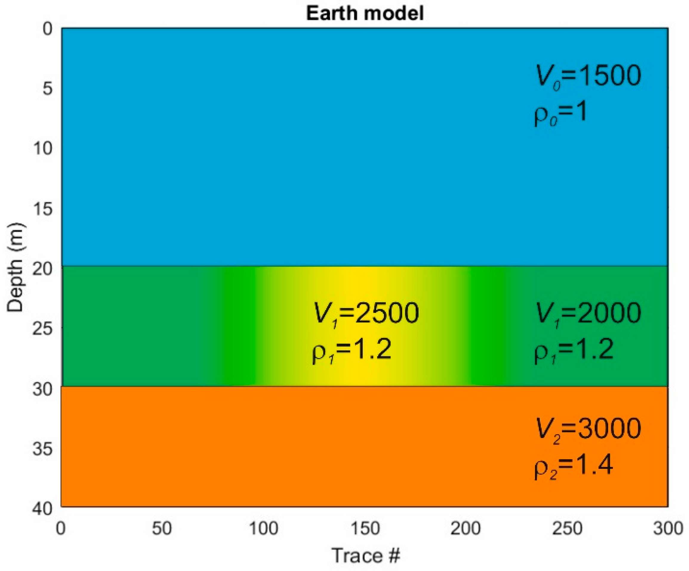
Figure 1. Parameters of a 1D Earth model. This model is composed of horizontal flat layers—seawater (light blue), sediment (green) and deeper layer (brown)—that are homogeneous in the vertical direction.
Jmse 12 00588 g001
Figure 2. Ray paths of the multiple reflections used for the traveltime and amplitude inversion, joining source (asterisk) and receiver (gray square). Peg-leg (a), intra-bed (b), simple (c), first reverberation (d) and second reverberation (e).
Jmse 12 00588 g002
Figure 3. Incidence angles for primaries and some multiples. The angles are: b for the seafloor primary (solid black line); a1 for the peg-leg multiple (dashed red line); a2 for the intrabed multiple (cyan dashed line); and a3 for the simple multiple (dotted green line). The incident angles ai are different for each multiple type.
Jmse 12 00588 g003
Figure 4. Intersection line (black dots) between two surfaces in the 3D solution space. The dimensions are thickness, velocity and density. The red surface defined by (9) includes solutions with a given one-way transit time across the sediment layer, while the blue surface defined by (10) includes solutions with a given acoustic impedance.
Jmse 12 00588 g004
Figure 5. Main parameters of Model 1, composed of layers of water (blue), sediments (green and yellow) and basement (brown). The colors highlight the central high velocity anomaly in the sediments, while the density does not change in any layer.
Jmse 12 00588 g005
Figure 6. Estimated thickness, P velocity and density of the sediment layer and the water depth. We inverted the traveltimes and amplitudes simulated in Model 1 (Figure 5) and added random noise of ±1% to their values. For the smoothing, we used a median filter of 31 samples. The dashed lines show the true Earth model, the solid blue lines represent the unsmoothed estimates, and the dotted red lines represent the smoothed version.
Jmse 12 00588 g006
Figure 7. Estimated thickness, P velocity and density of the sediment layer and the water depth. We inverted the traveltimes and amplitudes simulated in Model 1 (Figure 5) and added random noise of ±1% to their values. For the smoothing, we used a median filter of 71 samples. The dashed lines show the true Earth model, the solid blue lines represent the unsmoothed estimates, and the dotted red lines represent the smoothed version.
Jmse 12 00588 g007
Figure 8. Main parameters of Model 2, composed of layers of water (blue), sediments (green and white) and basement (brown). The colors highlight the central low-velocity anomaly in the sediments, which affects both velocity and density. A vertical fault introduces sharp discontinuities in the Earth parameters, i.e., water depth and thickness, velocity and density of the sediment layer.
Jmse 12 00588 g008
Figure 9. Estimated thickness, P velocity and density of the sediment layer, and water depth. We inverted the traveltimes and amplitudes simulated in Model 2 (Figure 8) with a percentage noise level of 0.1% and applied a median filter with 31 samples. The dashed lines show the true Earth model, the solid blue lines represent the unsmoothed estimates, and the dotted red lines represent the smoothed version.
Jmse 12 00588 g009
Figure 10. Estimated thickness, P velocity and density of the sediment layer, and water depth. We inverted the traveltimes and amplitudes simulated in Model 2 (Figure 8) with a percentage noise level of 0.3% and applied a median filter with 31 samples. The dashed lines show the true Earth model, the solid blue lines represent the unsmoothed estimate, and the dotted red lines represent the smoothed version.
Jmse 12 00588 g010
Figure 11. Comparison of different smoothing filters. The Savitzky–Golay (left) and median filter (right), both with a length of 31 samples, stabilize the LV1 term, i.e., the one-way traveltime through the sediments. In both cases, the scaled estimate (dotted red lines) fits the true model (dashed yellow lines) better than standard smoothing (solid blue lines).
Jmse 12 00588 g011
Figure 12. Seismic section obtained by a Boomer profile after a bandpass filter of 200–4000 Hz to remove the frequencies most affected by noise. Several diffractions due to plumes are evident in the water layer between 0 and 50 ms. The main reverberations due to the seafloor are well evident at 50, 100 and 150 ms.
Jmse 12 00588 g012
Figure 13. Seismic data as in Figure 12 after compensation for the geometrical spreading of the water layer. We picked traveltime and amplitude of the seafloor (red line), the base of sediments (yellow line), the first multiple of the seafloor (green line), the peg-leg multiple of the sediment’s base (pink line) and the second multiple of the seafloor (blue line).
Jmse 12 00588 g013
Figure 14. Inversion results from the amplitudes and traveltimes picked in Figure 13. Dotted blue lines show the preliminary inversion results without the smoothing filter, and the dashed orange lines the smoothing output.
Jmse 12 00588 g014
Figure 15. Block diagram for data processing and error propagation. Traveltimes and amplitudes (gray boxes) are the data that are inverted for the P velocity and acoustic impedance of the sediments. The intermediate steps of smoothing and scaling (blue boxes) can be repeated several times in order to finally obtain the estimated density and velocity (yellow boxes).
Jmse 12 00588 g015
Table 1. Parameters of Model 1 in Figure 5.
Layer NameVelocity (m/s)Density (g/cc)Thickness (m)
Seawater1500120
Sediments2000–25001.210
Basement30001.4-
Table 2. Parameters of Model 2 in Figure 8.
Layer NameVelocity (m/s)Density (g/cc)Thickness (m)
Seawater1500115–25
Sediments1600–20001.1–1.37–10
Basement30001.4-
Disclaimer/Publisher’s Note: The statements, opinions and data contained in all publications are solely those of the individual author(s) and contributor(s) and not of MDPI and/or the editor(s). MDPI and/or the editor(s) disclaim responsibility for any injury to people or property resulting from any ideas, methods, instructions or products referred to in the content.

