Article

Three-Dimensional Turbulent Simulation of Bivariate Normal Distribution Protection Device

1
Institute of Port, Coastal and Offshore Engineering, Ocean College, Zhejiang University, Zhoushan 316021, China
2
Zhejiang Ocean Blue Marine Planning and Design Co., Ltd., Hangzhou 310058, China
3
College of Architecture and Civil Engineering, Zhejiang University, Hangzhou 310058, China
*
Authors to whom correspondence should be addressed.
These authors contributed equally to this work.
J. Mar. Sci. Eng. 2024, 12(4), 602; https://doi.org/10.3390/jmse12040602
Submission received: 26 February 2024 / Revised: 21 March 2024 / Accepted: 24 March 2024 / Published: 30 March 2024
(This article belongs to the Section Ocean Engineering)

Abstract

:
In response to the deficiencies in existing bridge pier scour protection technologies, this paper introduces a novel protective device, namely a normal distribution-shaped surface (BND) protection devices formed by rotating a concave normal curve. A three-dimensional turbulent SST k ω model is constructed, and physical model experiments of conical surfaces are conducted to validate the mathematical model. The simulation analyzes longitudinal water flow, downflow, vorticity intensity, and shear stress within normal and conical surfaces. The results show that the downflow distribution in front of the pier spans a relative water depth of (−0.45, 0.67), with a peak velocity approximately 70% of the longitudinal flow velocity. Circulation forms within the surfaces, with the main vortex flux inside the BND being 33% lower than that inside the conical surface. The maximum shear stress coefficient inside the BND can reach 9, and the protective surface isolates the bed from the flow to prevent scouring by high shear stress. The velocity gradient at the edge of the surface is small, and the edge shear stress of the 3D normal distribution-shaped surface (BND) protection device is only one-third of that of the conical surface, preventing edge scouring. The large shear stress and its distribution area decrease monotonically with the increase in surface width. When the surface width is four times the diameter, the distribution range of the shear stress coefficient greater than 1 is very small. The study of three-Dimensional turbulence within the BND provides a numerical basis for an anti-scour design.

1. Introduction

Bridge foundations are mostly located in environments with deep water, rapid flow, and complex geological conditions. Due to the presence of bridge foundations, the cross-sectional area for water flow is reduced, obstructing the flow and inevitably altering the structure of the water flow and sediment movement, making scouring phenomena increasingly prominent. Over time, water damage adversely affects the safety and stability of bridges [1,2,3]. Local scour is influenced by such factors as hydraulic characteristics, sediment movement, and the form and arrangement of foundation structures [4,5,6]. Local scour around bridge piers is mainly caused by three factors: (1) The obstruction of water by bridge piers leads to an increase in longitudinal flow velocity, meaning that when water flow encounters an obstacle, the cross-sectional area for water flow decreases, resulting in an increase in local flow velocity and scouring of the bed sediment to form a scour hole; (2) the advancing water flow collides with the bridge pier, forming a stagnation point on the water surface in front, creating a top-down pressure gradient, and the resulting downflow directly erodes the bed surface [7,8]; (3) the horseshoe vortex formed when water flows around the obstacle carries away some of the sediment around the pier [9,10,11].
Ensuring the safe and stable operation of bridges is an urgent issue that needs to be addressed. Appropriate protective measures must be taken to ensure the safety and stability of hydraulic projects [12]. Based on the principle of protection, bridge pier scour protection measures can be divided into two major categories: passive protection and active protection [13]. Passive protection mainly refers to placing solid materials around the bridge piers to change the hydraulic characteristics of the incoming flow, such as riprap protection and grouted riprap. Traditional protection methods are based on passive protection concepts, but due to the poor protection effect and high maintenance costs associated with enhanced eddies, there is now a gradual shift towards active protection methods. Active protection mainly involves changing the structure of the bridge pier itself to enhance the scour resistance of the riverbed around the pier and altering the hydrodynamic conditions to weaken or suppress scouring through engineering measures, mainly including horizontal collars and slot protection [14]. The efficiency of slot protection significantly decreases when the direction of the approaching flow is not aligned with the direction of the slots [15]. A good protection effect is achieved when active and passive protections are combined. Mou et al. [16] explored the protective effect of the combination of ring-wing anti-scour plates and slots, and the reduction rate of the scour hole depth was 1.8 times that of slot protection. Sun et al. [17] studied the factors influencing local scour under bridges with shallow foundations and downstream protection dams and found that controlling the bottom slope of the dam body between −0.011 and −0.022 yielded better protection results.
In recent years, international scholars have conducted in-depth studies on the protective effects of collars. Tafarojnoruz et al. [18,19] summarized the active protection of bridge piers and explained the characteristics of the flow field around the piers and the practical application effects of engineering projects. Collars are generally 2–4 times the diameter of the bridge pier and have a small thickness [20]. When the collar diameter is 4 times the diameter of the bridge pier and the installation position is at the initial bed height, the scour depth can be reduced by up to 55% [21]. Pandey et al. [22] conducted flume experiments on collar protection under clear water scour conditions, and the results showed that the local scour depth decreases with the reduction in the collar installation height and the increase in the collar diameter. Alabi et al. [23] conducted a long experiment of about 40 days, and the results showed that collars can not only reduce the equilibrium scour depth but also slow down the scouring process. To increase the protection efficiency of collars, Tang et al. [24] proposed a prediction equation for the equilibrium scour depth of a single pile under collar protection and a formula for the protection efficiency.
Changing the shape of the collar also has certain improvements on the protective performance. Chen et al. [25] proposed a new type of hook-shaped collar and analyzed it through numerical simulation with a width of 1.25b and a height of 0.25b, where b is the bridge–pier width. Compared with the unprotected case, the horseshoe vortex intensity and the maximum turbulent kinetic energy are minimized at a burial depth of 0.25b, reducing the scour depth by 50%. Valela et al. [26,27] developed an innovative collar design named CPN3. Numerical simulations have shown that the unique three-dimensional ring structure of CPN3 effectively weakens the horseshoe vortex and the flow velocity near the bridge piers, resulting in a reduction of the maximum scour depth by 69.7%. [26,27]. Ettema et al. [28] presented a contemporary approach to scour-depth estimation, combining semiempirical formulation, advanced experimentation, and computational fluid dynamics (CFD), reflecting on the evolution of understanding complex pier flow fields over the past six decades and suggesting areas for further research to enhance design estimation of scour depth. Bento et al. [29] numerically investigated the complex flow structure and sediment entrainment mechanisms around an oblong bridge pier using the Sediment Simulation in Intakes with Multiblock option (SSIIM) computational fluid dynamics (CFD) tool, aiming to accurately reproduce measured scour depths with an average relative error of less than 3%.
Currently, improvements in collar scour protection measures are mainly focused on the cross-sectional shape, and edge scouring may still occur after improvement, with few studies and analyses on three-dimensional water flow [30]. This paper conducts three-dimensional water flow numerical simulations of the novel BND protection device and compares it with a conical surface formed by rotating a straight line.

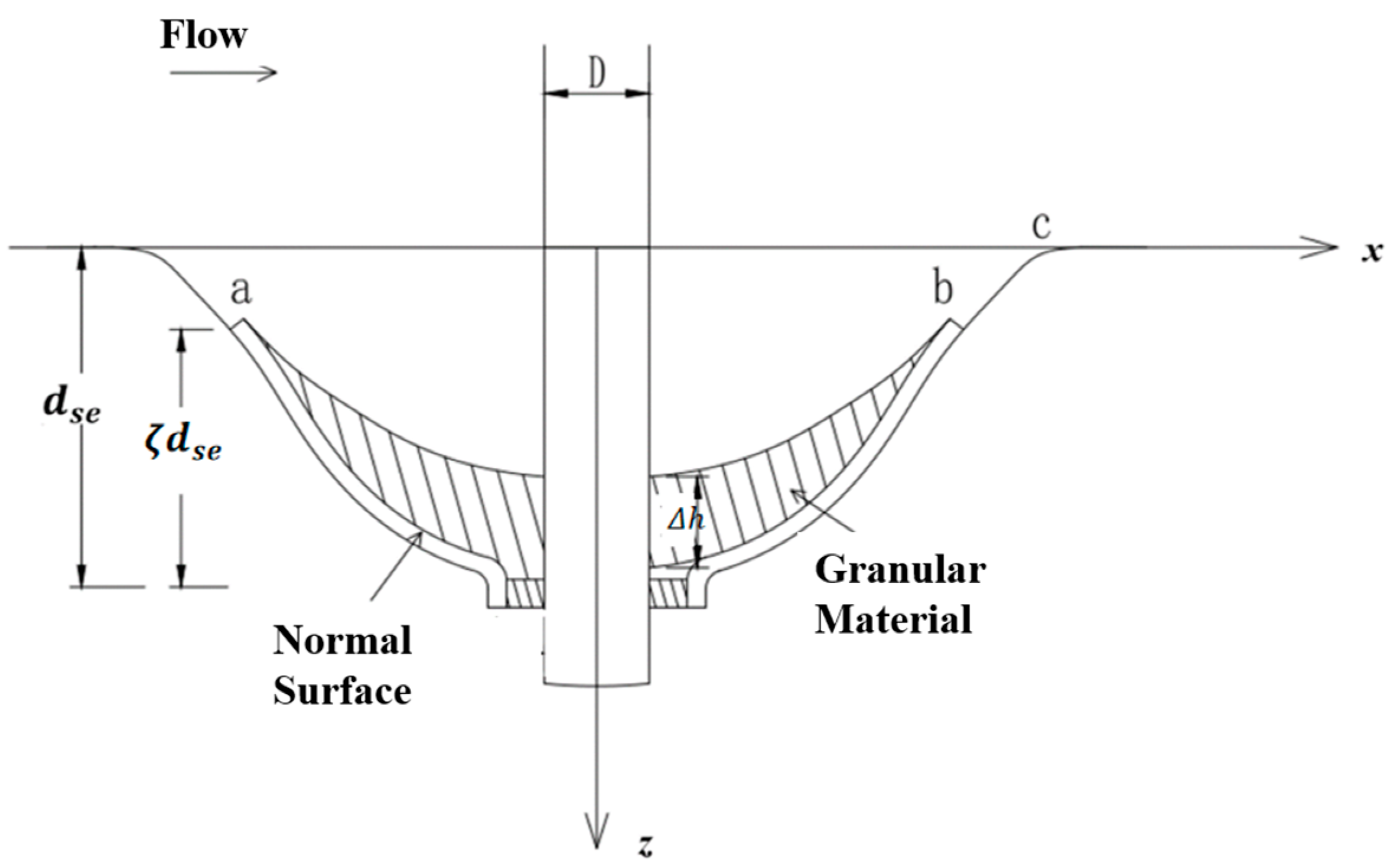
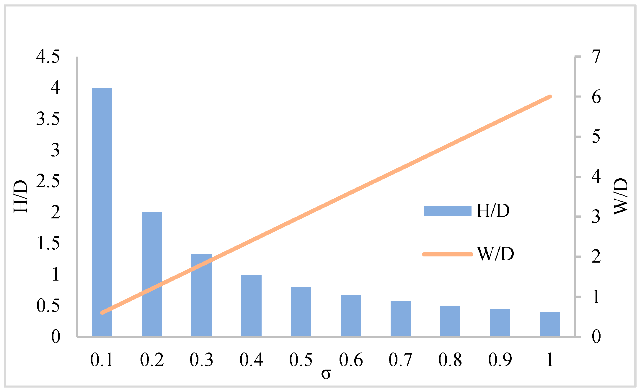
2. Protection Device in the Shape of a Bivariate Normal Distribution (BND)

Starting from the mechanism of local scouring, Sun Zhilin invented a bridge pier scour protection structure combining a concave rotating BND with granular materials, which can be used for local scour protection of sea-crossing bridges [31]. When the local scour hole around the bridge pier reaches a set depth close to equilibrium, the water flow and sediment movement in the scour hole are relatively weak. By laying a rotating BND protection structure resembling an “inverted bell”, the excellent property of continuous derivatives of any order of the BND is utilized to effectively deflect the descending water flow away from the bridge pier, thus weakening the impact of the descending flow on the bed surface. A specific thickness of granular material is laid inside the concave BND to reduce the horseshoe vortices around the bridge pier. The combination of the BND and the granular layer can resist the impact of the descending flow and eliminate the scouring action of the horseshoe vortices, providing effective protection against scouring of the bridge foundation. This design principle has a guiding role in the protection against scouring of the foundations of water-related structures. To ensure that the particles are not removed from the protection structure, the sum of the work done by the hydrodynamic force and buoyancy should be less than the work done by gravity and surface resistance. The granular material is not the focus of this paper, so it is not elaborated on. The local scour protection device is shown in Figure 1.
The inner surface of the BND shell satisfies the following equation:
z = k 2 π σ e x p ( ( x μ ) 2 + ( y μ ) 2 2 σ 2 ) , x 2 + y 2 > D 2 + l
In Equation (1), the positive direction of the x-axis is the direction of the water flow; the y-axis is perpendicular to the water flow; the z-axis is along the axis of the bridge pier, with the positive direction upwards, and the origin is the intersection of the center of the bridge pier and the unscoured bed surface. σ is the standard deviation parameter of the BND; the bottom of the BND is located at m d s e below the bed surface, d s e is the maximum scour hole depth, m = 0.7–0.9, and μ = D / 2 is the radius of the bridge pier; k is a scaling factor related to depth.
The ratio k/σ adjusts the height of the normal distribution surface. As shown in Figure 2, for the standard deviation σ from 0 to 1, the changes in the width W/D and height H/D of the BND are shown in the figure. As the standard deviation σ increases, W/D increases linearly, while H/D gradually decreases. This does not conform to the morphological rule of the bridge pier scour hole, so k is introduced to adjust the height, which can achieve any height desired by the designer, helping in the design of the surface. The clear water scour depth is always less than 2.3 times the diameter of the bridge pier, while the movable bed scour depth is always less than 2.0 times the diameter of the bridge pier. Therefore, the range of σ can be taken between 0.2 and 0.5.
In this paper, the scour depth is calculated using the formula from Hydraulic Engineering Circular No. 18 (HEC-18) proposed by Richardson (2001), which is applicable to both clear water and live bed scour [32]. Arneson further optimized the HEC-18 formula [33] by introducing shape factors and hydraulic conditions based on new experimental data, and its expression is as follows:
d s e H = 2.0 K 1 K 2 K 3 ( D H ) 0.65 F r 0.43
where K 1 is the pier shape coefficient (circular pier is 1); K 2 is the flow angle coefficient (orthogonal flow is 1); K 3 is the bed form coefficient (clear water scour and small dune is 1.1); Fr is the Froude number of the flow.

3. Three-Dimensional Turbulent Mathematical Model of BND

3.1. Control Equations

The three-dimensional water flow around the BND follows the Navier–Stokes (N-S) equations [34]:
ρ t + ρ u i x i = 0
ρ u i t + x j ( ρ u i u j ) = p x i + μ x j [ u j x j + u j x i ] + x j [ ρ u i u j ¯ ]
where t is time; in the Cartesian coordinate system, x i = ( x , y , z ) , u i = ( u x , u y , u z ) are the coordinates; p is the pressure; ρ and μ are the density and dynamic viscosity of the water, respectively; u i and u j are the fluctuating velocities corresponding to x i and x j ; ρ u i u j ¯ is the Reynolds stress. Due to the addition of six Reynolds stresses, a turbulence model needs to be introduced to close the equation set.
The k ω model can calculate fully developed turbulent flow in the far field and the near-wall boundary layer problem under a pressure gradient. The SST k ω (shear stress transport) model combines the advantages of both far-field and near-wall boundary layer problems [35]. It extends the applicable range from the turbulent core region to the near-wall region, mainly solving for the turbulent kinetic energy k and specific dissipation rate ω = k / ε , whose control equations [36] are as follows:
ρ k t + x j [ ρ u j k ( μ + σ k μ t ) k x j ] = τ t i j S i j β ρ ω k
ρ ω t + x j [ ρ u j ω ( μ + σ ω μ t ) ω x j ] = P ω β ρ ω 2 + 2 ( 1 F 1 ) ρ σ ω ω k ω x j x j
The eddy viscosity model for the corresponding Reynolds stress is as follows:
τ t i j = 2 μ t ( S i j S n n δ i j 3 ) 2 ρ k δ i j 3
where μ t = ρ k / ω is the eddy viscosity coefficient; S i j is the mean velocity strain rate tensor; δ i j is the Kronecker delta. P ω is the production term:
P ω = 2 γ ρ ( S i j ω S n n δ i j 3 ) S i j
The model parameters are set as follows, where subscripts 1 and 2 represent the inner and outer regions, respectively:
σ k , 1 = 1.176 , σ k , 2 = 1.0 , σ ω , 1 = 2.0 ,   σ ω , 2 = 1.168
β i , 1 = 0.075 , β i , 2 = 0.0828 , a 1 = 0.31 , β = 0.09
Equations (7) and (8) are discretized using the finite volume method (FVM), and the coupling of velocity and pressure is solved using the PISO algorithm. In spatial discretization, gradients are based on the least squares method for cells, and momentum, turbulent kinetic energy, and dissipation rate all use a first-order upwind scheme. To prevent divergence and instability in the numerical calculation during the iteration process, under-relaxation techniques are used.

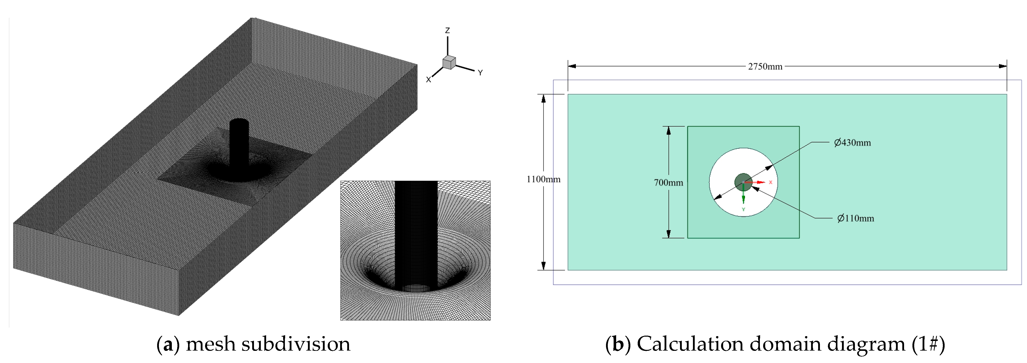
3.2. Geometric Model and Mesh

Assume that the diameter of the bridge pier is D, the distance on both sides of the pier is 4.5D, and the downstream distance is 12D to ensure that the outer boundary is not affected by the flow around the pier, of which the water flow is along the x-axis direction. The size of the computational domain is 25D × 10D × 3D, as shown in Figure 3. When the ratio of water depth to pier diameter H/D > 2.5, the influence of the free surface on the flow field is small, which conforms to the rigid lid assumption [37]. The left boundary is set as a velocity inlet, the right boundary is set as a pressure outlet, the sides and top of the flume are set as symmetric boundary conditions, and the bottom is a wall boundary. The BND surface possesses a smooth surface, while the bed possesses a roughness ( k s ) of 0.16 mm, which is defined within the wall functions.
The computational domain uses nine blocks of three-dimensional hexahedral structured grids, with a dense O-type grid generated on the protective surface. The grid size for the entire field is set to 1 cm, with an orthogonality of no less than 0.9. The model grid is nested to achieve local refinement, dividing the computational domain into inner and outer layers, with the inner layer grid being a rectangular area of 0.7 m × 0.7 m. Using the formula x i *   = 0.172( x i /D)Re0.9 to back-calculate the thickness of the first layer of the boundary layer grid, when x i = 3, the thickness x i = 0.02 cm. The wall grid is refined according to x i , with a growth rate of 1.05. The number of grids in the x, y, and z directions are 346, 185, and 50, respectively, with a total of 2,782,806 grids.
For explicit calculations, the time step should satisfy the CFL condition. Equation (9) is as follows:
C = Δ t i = 1 n u m a x Δ x i 1
where C is the Courant number; u max is the maximum flow velocity; Δ x i is the minimum grid size; Δ t is the time step, set Δ t = 5 × 10 4   s   <   8 × 10 4   s , and the total calculation duration is set to 100 s.

3.3. Mathematical Simulation Scheme

In the numerical simulation, the diameter of the bridge pier is set as D = 0.11 m, based on the HEC-18 formula, and the maximum scour depth d s e = 0.13   m . The surface design depth, calculated according to the above formula, is d s e = 1.27 D . The value of H/D is taken as 70% of the maximum scour depth, which is 0.9D.
For the convenience of modeling, the BND is formed by the rotation of a normal curve, satisfying the following equation:
z s = k 2 π   σ exp ( x s 2 2 σ 2 )
Using a conical surface as a reference, the three-dimensional water flow numerical simulation results of cases #1 and #2 are compared to explore the water flow characteristics of the BND. Cases #2 to #5 vary the width W of the BND to explore the impact of different protection ranges on the water flow around the pier. The simulation scheme is shown in Table 1.
As shown in Figure 4, the BND is obtained by rotating a custom function curve in the modeling software, SolidWorks 2020. Taking W = 3.9D as an example, when σ and k are set to 0.5 and 1.25, respectively, Equation (11) is as follows:
z s = 2.5 2 π   exp   [ ( x s 0.55 ) 2 2 × 0.5 2 ] , x s [ 0.55 , 2.15 ]
The local scour home around the bridge pier is generally conical in shape, with the side slope approximately equal to the underwater angle of repose. The parametric equation for the conical surface in case #1 is a straight line, as follows:
z = 0.625 k 1.34 ,   x [ 0.55 , 2.15 ]

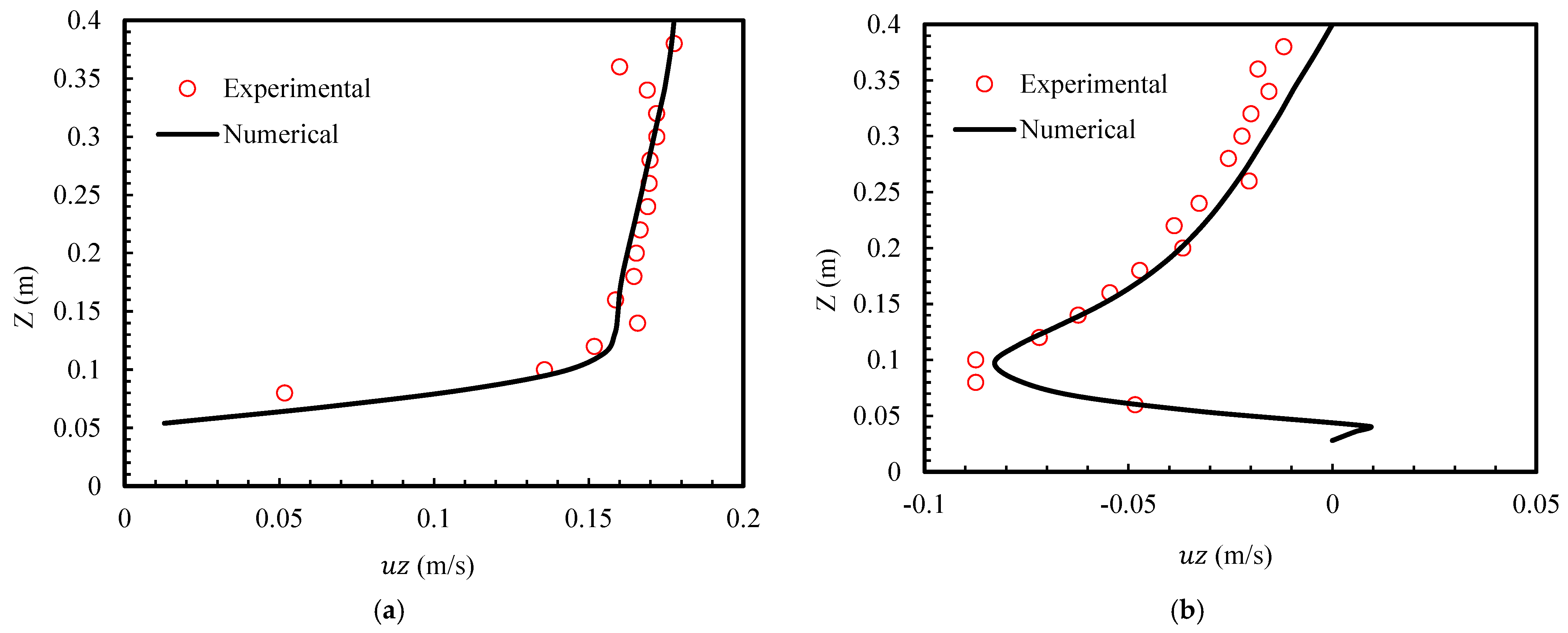
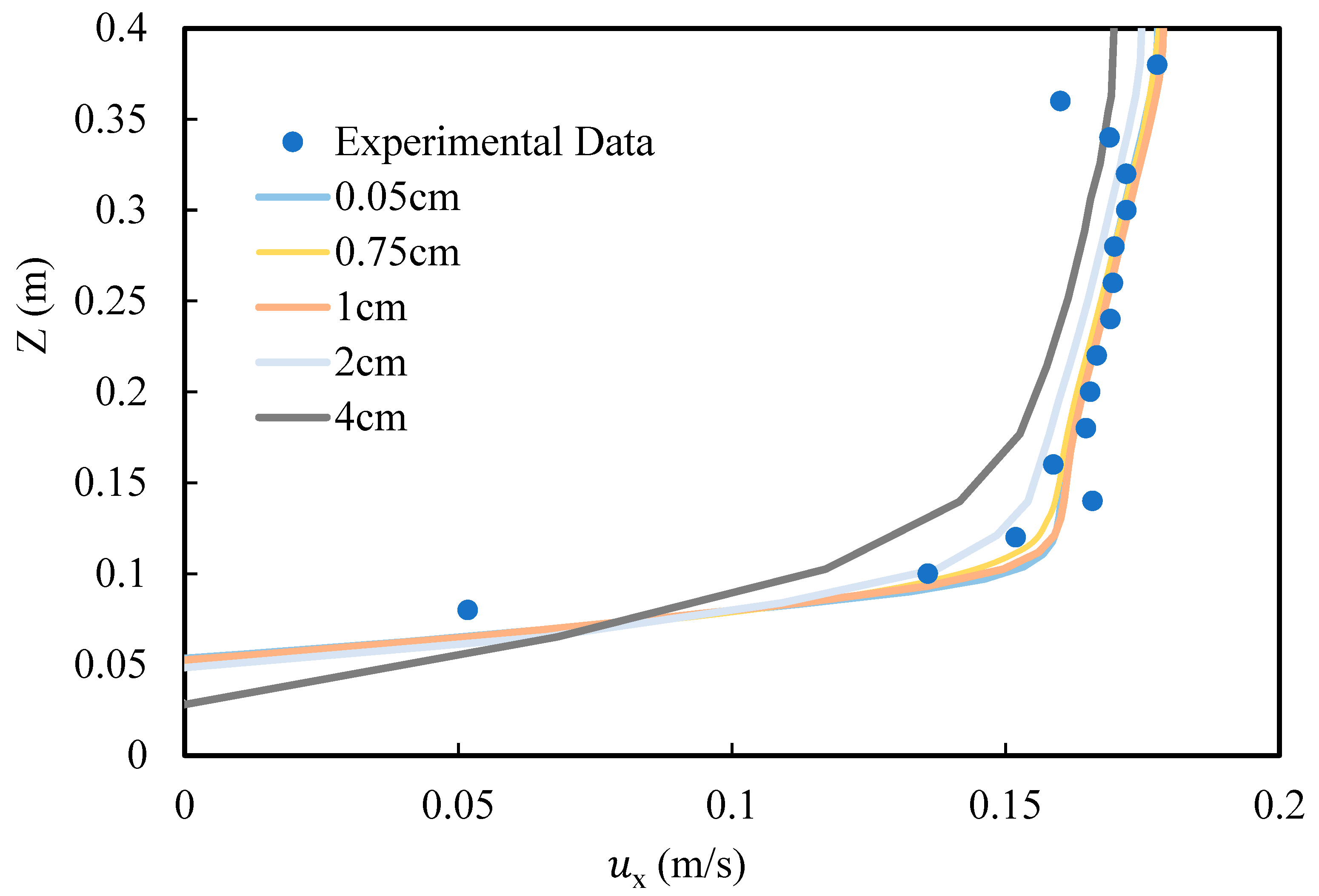
3.4. Validation of the Mathematical Model Based on Experiments

Previous experiments have found that the scour hole around bridge piers is generally conical in shape, with the slope of the sidewalls approximately equal to the angle of repose underwater. To verify the numerical model, we conducted physical model experiments on the flow around pile foundations in a multifunctional flume at the Zhejiang University Construction Testing Hall. The flume is 69.0 m long, 1.2 m wide, and 1.6 m high. The model bridge piers are made of PVC material with a diameter of D = 0.11 m and are fixed to the bottom through the sand layer with bolts. When B/D > 8.0, the influence of the flume sidewalls on the flow and scour can be neglected. The water depth is controlled at H = 0.3 m, and the median grain size of the natural quartz sand is d 50 = 0.16   mm . The experimental flow is a constant uniform flow, with the average flow velocity U 0 = 0.25   m / s along the water depth measured at the centerline of the flume upstream of the pile. To simulate the most unfavorable condition for the scour of a single pile foundation, the experiment used unidirectional flow clear water scouring.
To verify the flow conditions, the flow velocity distribution along the vertical direction at 1 m upstream of the bridge pier was measured using an acoustic doppler velocimeter (ADV). The time-averaged flow velocity is shown in Figure 5, and the experimental results agree well with the theoretical curve. The logarithmic velocity distribution is used as the inlet boundary condition for the numerical model in the form of a user-defined function (UDF).
u U = 2.5 ln ( 30 z k s )
In the flow field data of the physical model experiment and numerical simulation scheme #1, the velocity profiles at x/D = −1 in front of the pier are selected for comparison. The positions of the experimental measurement points are meticulously illustrated in Figure 6. Subsequently, the outcomes derived from both the experimental investigation and the numerical simulation are comprehensively presented in Figure 7, facilitating a detailed comparison and analysis. The root mean square error (RMSE) RMSE = 1 n i = 1 n ( y i ^ y i ) 2 = 0.006   m / s , indicating a high degree of fit. This demonstrates that the numerical model in this paper is scientifically reliable. The simulated longitudinal and vertical velocities are in good agreement with the measured data and can be used for the flow field simulation of the novel BND protection.

3.5. Grid Independence Verification

To verify the rationality of grid mesh and parameter settings and save computational resources, this paper uses five different resolution grids for calculation, with grid sizes of 4 cm, 2 cm, 1 cm, 0.75 cm, and 0.5 cm, respectively. The vertical distribution of the time-averaged longitudinal velocity at x/D = −1 in front of the pier in the numerical model is extracted and compared with the physical model data, as shown in Figure 8. The results indicate that when the grid size is smaller than 1 cm, the calculated flow velocity is in good agreement with the measured values. Considering computational efficiency, a grid size of 1 cm is chosen, which meets the requirements of grid independence and convergence while maintaining high computational efficiency.

4. Turbulent Characteristics of the BND

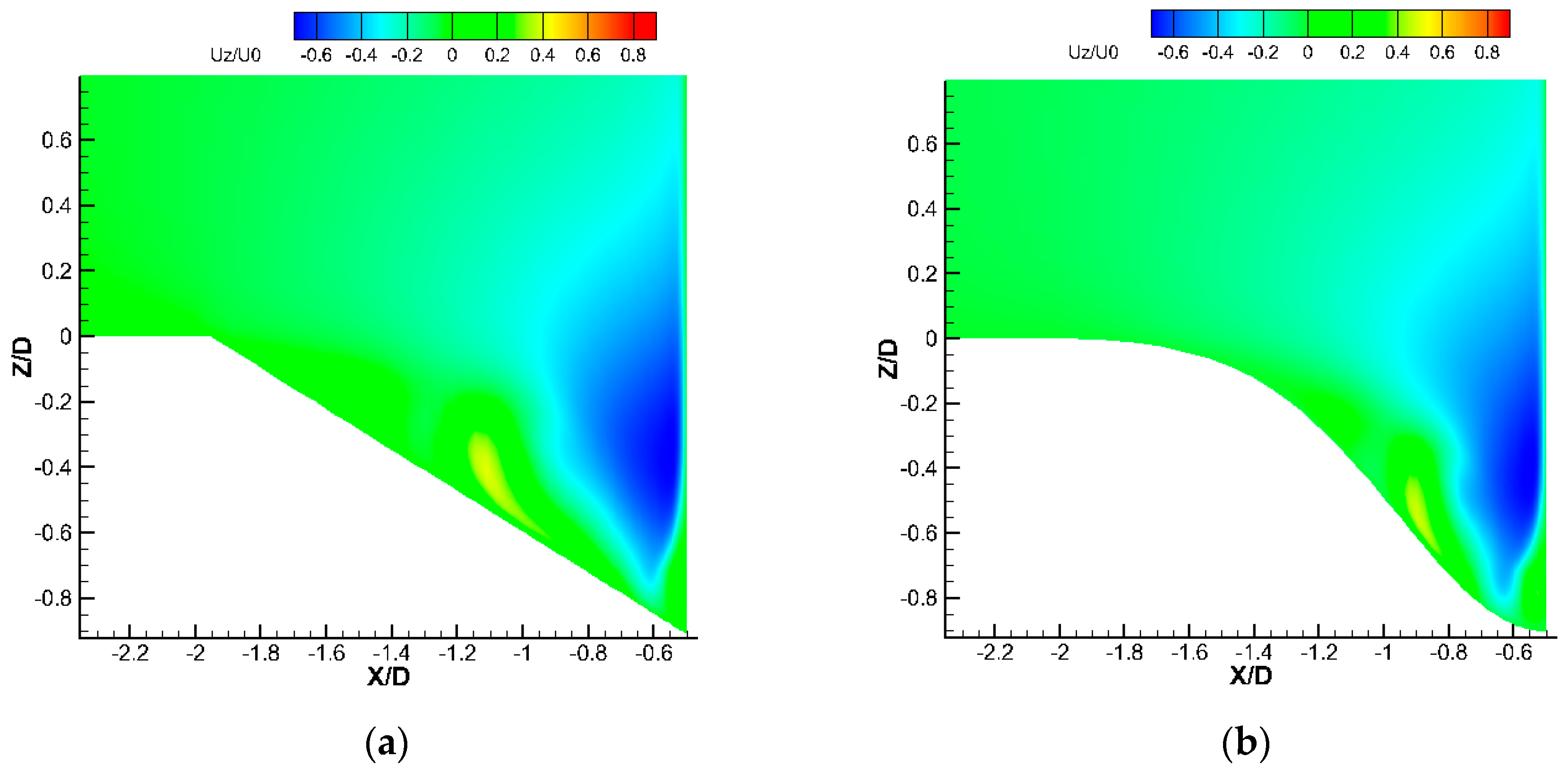
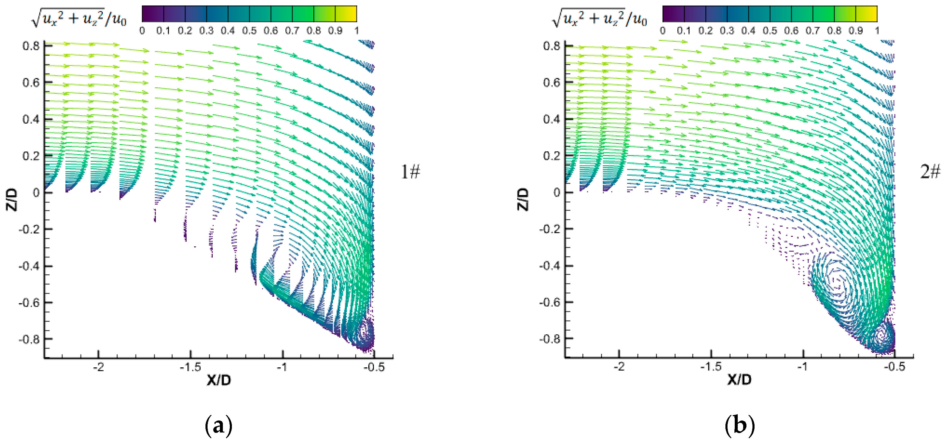
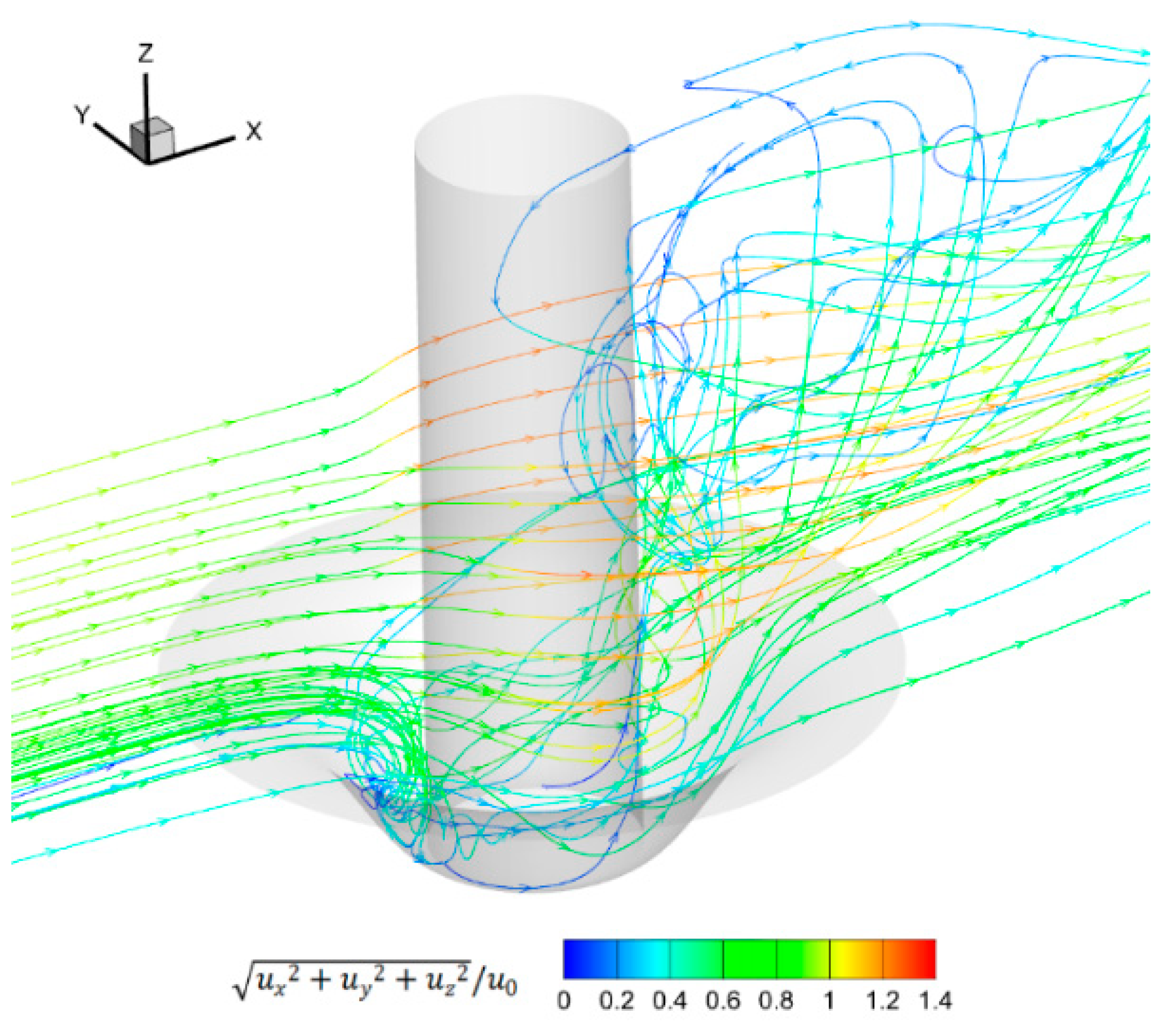
4.1. Analysis of Velocity Characteristics

The gradient of velocity near the bed reflects the strength of the water flow’s action on the bed. To analyze the velocity distribution near different protective beds, the lateral distribution of longitudinal velocity at z = 1 cm and z = 0.6H on the cross-section at x/D = 0 is selected and plotted in Figure 9. The horizontal coordinate is the relative distance y / D , and the vertical coordinate is the non-dimensional longitudinal velocity u x ( y ) / U 0 .
The incoming flow is affected by the reduction in the cross-sectional area of the bridge pier, and the maximum longitudinal velocity appears at x = 0.6D. According to the data in Figure 9a, the closer to the center line of the bridge pier, the greater the extreme value of the bottom longitudinal velocity, but the velocity change is within the range of the surface, so it does not affect the disturbance of the bed.
Comparing the velocity gradients at the edge of the surface, at x = 1.9D, the lateral gradients of longitudinal velocity du/dy for cases #1 and #2 are −0.48 and −0.43, respectively, indicating that the water resistance of the conical surface is greater than that of the BND, with more severe velocity changes, more apparent relative motion between layers of fluid, and greater shear forces.
In Figure 9b, at z = 0.6H, the impact of the bridge pier on the time-averaged longitudinal velocity is shown, with little difference in the upper water body among the different cases. At y / D = 2.5 , and u x ( y ) / u 0 = 1.01 , which means that the longitudinal velocity is approximately equal to the incoming flow velocity. This indicates that the width of the water flow significantly affected by the bridge pier is about 5 times the diameter of the pier, and when the lateral distance from the pier is sufficiently far, the longitudinal velocity is not affected by the pier.
Figure 10 shows the velocity contour maps of the longitudinal section upstream of the bridge pier for cases #1 and #2. When approaching the bridge pier, a downflow forms below the stagnation point, with a negative vertical velocity u z . The peak values of the downflow velocity in both surfaces are about 70% of the longitudinal velocity x / D ( 1 , 0.5 ) , mainly distributed in the vertical range of −0.45 < z/H < 0.67 in front of the pier. Near the bottom, oblique water flow occurs, leading to recirculation.
Considering that the flow field in front of the pier is the main factor affecting local scouring, the following analysis mainly focuses on the downflow in front of the pier. Both the normal and conical surfaces exhibit characteristics dominated by the downflow. The distribution pattern of the downflow in front of the pier is similar, increasing from top to bottom and then decreasing. The upper part of the vertical velocity distribution is uniform with little difference, and the main impact is concentrated on the flow structure in the middle and lower parts.
Figure 11 shows the distribution of vertical velocity at distances x = −0.68D, −1.1D, and −1.95D upstream of the pier. The peak downflow velocities on both surfaces vary in position.
At x = −0.68D perpendicular to the pier, the flow pattern changes around the pier can be accurately reflected. Comparing the two surfaces with the same width, the peak downflow velocity for case #2 is 0.54 U 0 , which is 0.04 U 0 less than that for case #1. On the vertical line at x = −1.1D, the flow direction reverses at a certain depth within the surface of case #1, with an upward velocity peak of 0.38 U 0 at the inflection point z = −0.42D, while the upward velocity in the BND of case #2 is smaller.
It can be seen that the velocity distribution in the BND is concentrated, which is caused by the concentrated dissipation of water flow due to the shape of the BND. At x/D = −1.95, where the protective surface meets the bed sediment, the main scouring of the bed occurs. Comparatively, the downflow at the edge of the BND is significantly smaller than that of the conical surface, with the maximum velocity point farther from the bed, resulting in better protection.
To further investigate the location of the boundary layer separation points of the two surfaces, the velocity vector distributions of the two surfaces are plotted, as shown in Figure 12. It can be seen that the flow at the edge of the conical surface is deflected by the adverse pressure gradient, causing boundary layer separation, which is a sudden boundary layer separation. The velocity gradient near the bottom and the turbulence intensity are high, which may trigger scouring outside the edge of the bed. On the other hand, due to the excellent derivative properties of the BND, the flow is deflected by the surface and continues to move along the surface for a certain distance before boundary layer separation occurs, which is a gradual boundary layer separation. The bottom flow at the edge is stable, with a small velocity gradient and turbulence intensity. Therefore, scouring is unlikely to occur at the edge of the BND, resulting in excellent protection.

4.2. Vorticity Field Analysis

The vorticity in the Y direction can be expressed as:
ω Y = u z w x
Equation (14) is discretized using the forward difference method, and the time-averaged vorticity in front of the pier in the XZ plane is calculated and plotted in Figure 13, with clockwise direction being positive. Figure 13 also shows the streamline distribution within the two surfaces, clearly reflecting the rotation direction of the flow and vortex.
Due to the adverse pressure gradient formed by the downflow being obstructed by the bridge pier and the bed, a separation zone is formed between the boundary layer and the bed, and a transverse axis circulation in front of the pier is formed under the combined action of vertical and longitudinal velocities. The analysis of the motion-related vortex structure in front of the pier is basically consistent, with the vortex structure presenting a spiral shape similar to the time-averaged streamlines, where the horseshoe vortex and the high vorticity value area largely coincide. There are two primary vortices, PV1 and PV2, with negative vorticity in the surface, as well as a reverse vortex, BAV, and a boundary vortex, JV, with positive vorticity. The time-averaged main horseshoe vortex PV1 is usually defined as the vortex structure upstream of the bridge pier with the largest size, strength, and longest duration.
The Stokes theorem (15) is applied to calculate the vortex flux Γ to characterize the vortex strength, as follows:
Γ = A ω Y d A
where A is the circulation of the main horseshoe vortex in the closed area. The closed area of the main vortex upstream of the pier is selected for calculation.
Comparing the size and position of the main vortex PV1 for the two surfaces. According to the formula, the normalized circulation vortex fluxes Γ / UD for cases #1 and #2 are 0.3 and 0.2 , respectively, with #2 being only 67% of #1, indicating that the vortex amplitude of case #2 is smaller. The main vortex of the BND is roughly located at (−0.8D, −0.5D); the vortex center of the conical surface is at (−D, −0.36D), a bit further from the pier. The width of the main vortex of the conical surface is 0.46D, which is 1.7 times larger than that of the BND. Without protection, the strong circumferential circulation near the bed surface would lead to sediment transport, while the streamlined design of the BND causes the vortex to circulate within the surface cavity, reducing the vortex intensity and effectively isolating the water flow from the bed surface.
The scouring around the pier is related to the vorticity intensity. However, the vorticity formula cannot distinguish between shear and rotation, nor can it comprehensively represent the evolution process of vortices of various scales. The Q criterion can identify the influence of the shear layer and qualitatively describe the characteristic quantity of vortices through the following mathematical definition:
Q = 1 2 [ ( u x ) 2 + ( v y ) 2 + ( w z ) 2 ] u y v x u z w x v z w y
where x , y , z are the three coordinate components in the Cartesian coordinate system; u , v , w are the velocity components in the x , y , z directions, respectively. As shown in Figure 13, when quantitatively analyzing the vortex structure, regions with Q values greater than 2 are displayed.
Q > 0 indicates that the rotation rate of the fluid is greater than the strain rate, with larger values indicating that the flow vortex structure is dominant, the vorticity intensity is greater, and the scouring effect on the bed surface is greater. As shown in Figure 14, the Q value contour map at Z = 1 mm near the bed surface reveals that a distinct spanwise vortex forms at the outer edge of the conical surface, with the Q value reaching 80 behind the pier. In contrast, the BND allows for a smooth transition of the flow, with no large-scale spanwise vortices at the edge of the surface, and a Q value of 0, indicating a strong resistance to scouring.

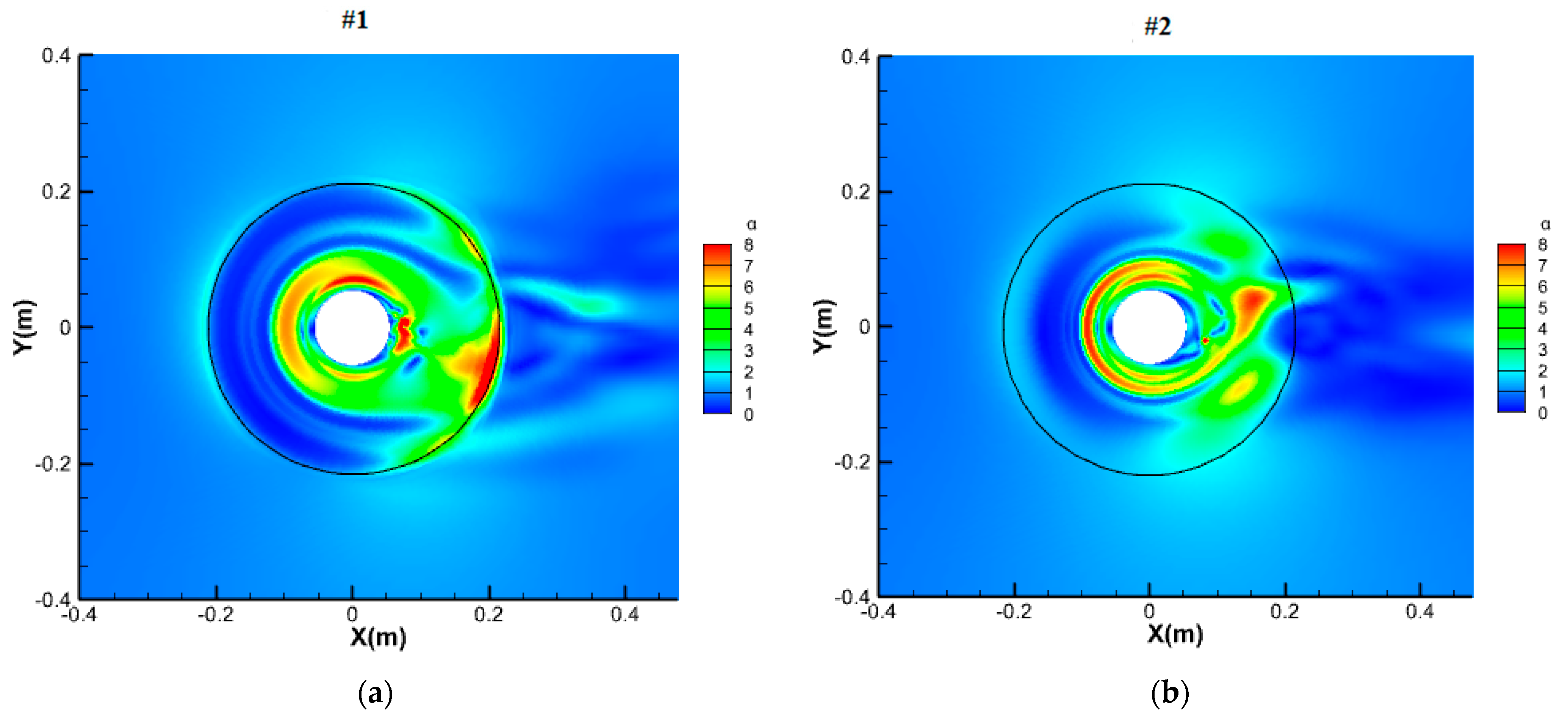
4.3. Analysis of Bed Shear Stress

When the water flow on both sides of the bridge pier is squeezed, the bed shear stress increases, easily causing scouring on the outer side of the surface. Bed shear stress τ is an important criterion for determining local scour around the pier, generally calculated directly from the k value near the bed based on the assumption that the generation and dissipation of turbulence reach equilibrium near the wall.
τ = c ρ k
Turbulent kinetic energy is calculated using the Soulsby [37] method.
k = 0.5 ( u 2 ¯ + v 2 ¯ + w 2 ¯ )
In Equation (15), c is a constant coefficient, taken as 0.19 ; u , v , and w are the horizontal, lateral, and vertical fluctuating velocities near the bed, respectively.
The bed shear stress amplification factor is as follows:
α = | τ τ |
where τ is the bed shear stress at the far end, unaffected by the bridge pier.
Figure 15 shows the non-dimensional bed shear stress contour maps for cases #1 and #2. The variations in bed shear stress around the conical and BNDs are compared and analyzed. The central angle θ in the flow direction is set to 0°. The maximum shear stress coefficients within the conical and BNDs reach 12 and 9, respectively, and the protective surface can prevent the bed from being scoured by high shear stress. The values α at the outer front edges of both surfaces are close to 1, with the value α at the outer rear edge of the conical surface being larger, varying between 4 to 9, distributed within a strip 1 cm wide in the range of 90° to 270° along the surface; the overall value α at the outer rear edge of the BND is less than 2, and the area of the range α ( 1.5 , 2 ] is smaller, the area of the range is 4   cm 2 with the edge shear stress being only one-third of that of the conical surface. This indicates that the shear stress around the BND is significantly smaller than that around the conical surface, which is beneficial for avoiding edge scouring.

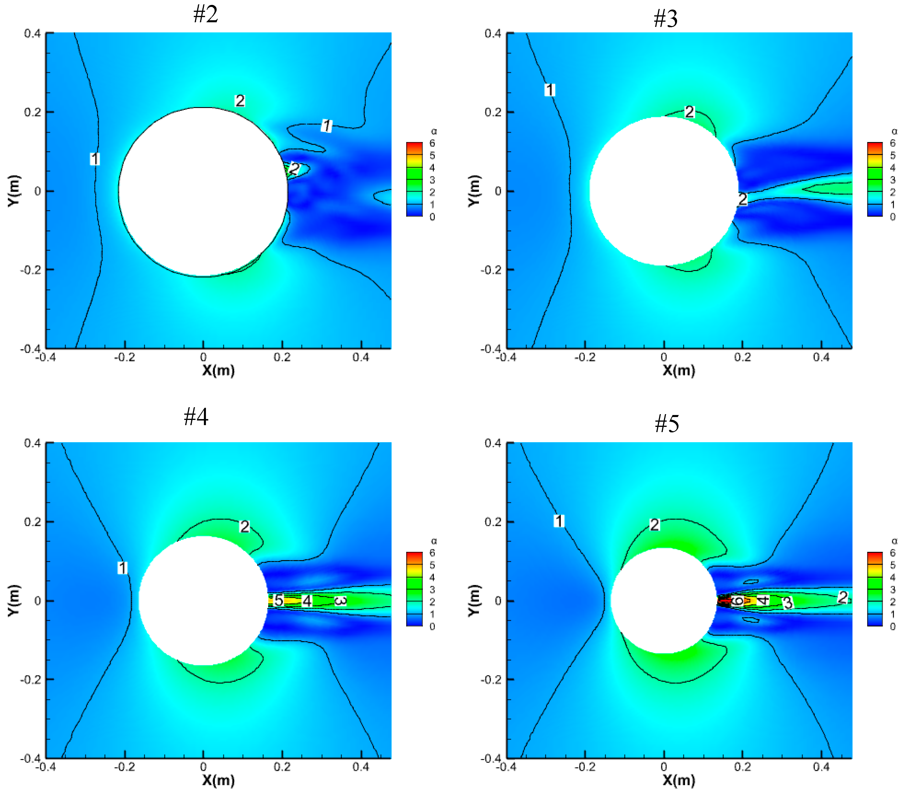
5. The Influence of the Width of the BND

The three-dimensional streamlines within the BND are shown in Figure 16. When the water flow is obstructed by the bridge pier, the protective surface wraps the downflow and horseshoe vortex around the pier, allowing the water to circulate within the surface, eliminating the scouring effect of the downflow and the flow around the pier side on the bed. The surface diversion causes the water flow behind the pier to flow obliquely at a certain angle, which also has a protective effect.
In cases #2 to #5 of the BND, the cross-section at x/D = 0 is selected, and the distribution of the longitudinal velocity at z = 1 cm along the lateral direction is shown in Figure 17. The maximum longitudinal velocity is U max / U 0 = 1.15~1.23, occurring at a distance of 0.09D from the pier. The flow velocity gradually decreases along the transverse direction, experiencing a sharp drop between y = 0.59D and 1.7D. Beyond y > 1.7D, the change in flow velocity becomes gradual. The overall trend of the longitudinal velocity distribution in the lateral direction is a rapid decrease followed by stabilization. The velocity gradients du / dy at the edge of the BND are 0.43 , 0.44 , 0.55 ,   and   0.69 , respectively, indicating that as the diameter of the BND decreases, the edge velocity gradient increases.
To quantitatively analyze the relationship between the variation in bed shear stress around the BND and the width of protection, Figure 18 shows the shear stress outside the BND, which is basically symmetrically distributed. As the width of protection W increases from 2.5D to 3.9D, the maximum shear stress coefficient outside the surface decreases from 6 to 2, showing a monotonically decreasing trend. Within the range of approximately 60° to 80° of the central angle on both sides of the surface, the distribution area of 1 < α < 2 significantly decreases as W decreases. When W 3.5D, the maximum shear stress coefficient on the rear side of the surface becomes α max = 2 , α ( 1 , 2 ] with a very small distribution area. When W = 4D, the distribution area of α = 2 is almost zero. This indicates that further expanding the protection range may have limited additional benefits for scour protection, so W = 4D can be considered a reasonable protection width. In actual engineering, the cost should be taken into account, and the width of the surface should be chosen to achieve the optimal protection effect.

6. Discussion

The novel protection device introduced in this paper, unlike traditional protective rings, can effectively guide the flow and block the downflow and weaken the horseshoe vortex without causing scouring. Valela et al. [26] proposed CPN3 through the improved protective ring (FPC), the core idea of which is to contain the horseshoe vortex in a concave cavity located below the riverbed, aiming to effectively reduce the scouring and sinking of the protective ring. Under all test conditions, CPN3 significantly reduced the scour depth ( d s ) and volume ( V s ) by at least 46.6% and 30.8%, respectively. The reason why CPN3 significantly improves the protective efficacy is that it can perform better under the conditions of reduced flow velocity or increased flow depth, showing its wide applicability as a bridge pier protection measure under different hydrodynamic conditions. Valela’s work focused on using numerical models to identify the bed shear stress around the protective ring, thereby revealing the possibility of scouring on both sides of the protective ring. This finding highlights the predictive ability of numerical models in simulating shear stress to predict scouring, further complementing our research on the evaluation method of the protective effect of BND.
The shape of CPN3 is similar to that of the BND, with both adopting a concave design, which demonstrates the effectiveness of this protection method. The advantage of this paper is that it provides equations and can adjust the shape according to the scour hole. This innovative design not only confirms the effectiveness of the concave geometric shape in protecting bridge piers from scouring but also provides a flexible solution that can be adjusted according to specific scouring conditions, further enhancing the application potential of the BND protection structure in bridge pier scour protection.
The maximum scour depth around bridge piers is influenced by the characteristics of the water flow ( ρ ,   μ ,   g ,   U ,   H ,   K T ), the properties of the riverbed sediment ( ρ s ,   d 50 ,   U c r ), and the geometric characteristics of the bridge pier ( D ). The design process for the BND is as follows:
(1)
With known parameters for the water flow, sediment, and bridge pier, we use existing empirical formulas or experimental data to calculate the maximum possible scour depth (dse).
(2)
We determine the height of the BND. If the actual scour hole has not reached the calculated value, we take the calculated height 0.7 des as the dimensional height of H/D. If the actual scour depth is greater than the calculated value, we take the actual value. However, the design value is generally larger.
(3)
We calculate the parameters k and σ for the BND.
Since 99.7% of the data in a normal distribution fall within μ 3 σ and μ + 3 σ , the non-dimensional width of the surface is set to W / D = 6 σ . The ratio of the hole width to the bridge pier diameter is provided by the numerical model in this paper, with the protection width relative to the bridge pier diameter ranging from 2 to 4.
When x = μ , the non-dimensional height of the BND is H / D = k 2 π σ . It is set to 90% of the maximum scour depth obtained from experiments or formulas, reflecting a measure of the relative depth of the scour hole. When σ increases, k decreases to maintain a constant depth.
Following the calculation of parameters k and c utilizing the outlined methodology, the construction methodology integrates both prefabricated assembly and cast-in-situ strategies for its components, opting for concrete as the material of choice. This approach endows the 3D near-bed scouring defense system (NDSS) with a design that is not merely innovative on a theoretical level but also exhibits significant practical applicability and adaptability.
In exploring the design and implementation of 3D near-bed scouring defense system (NDSS) protection strategies, the findings of this study exhibit notable correlations with the work conducted by Yagci et al. [38], which investigated scour patterns around isolated vegetation elements. The design of the BND, aimed at controlling water flow through a geometric shape to reduce scouring, can be seen as an engineering application extension of this concept. Similarly, the experimental evaluation of scour depths around spur dikes by M Pandey et al. [39] further confirmed the importance of geometric shapes in scour protection. Moreover, the novel normal surface spur dike structure proposed by Sun Zhilin et al. [40] indicates that streamline-shaped geometries can optimize surrounding water flow structures and reduce local scour. The cases in the literature provide a broad experimental background for the effectiveness of the BND protection design in this study, showcasing the potential application of the design in a variety of practical scenarios. Therefore, the innovative design of the BND protection structure is not limited to circular bridge piers but is expected to be widely applied to pier protection in various shapes and environments.
This paper only studies the surface through numerical results, lacking the ability to transport sediments, and does not consider the impact of sediment-laden flow on the scouring process, which may limit the general applicability of the results. Secondly, the designed protective ring model has only been tested and verified for circular bridge piers, and its application potential under other bridge pier shapes has not yet been explored. Therefore, future research needs to further explore the performance of protective rings under different hydrodynamic and sedimentary conditions, and to develop protective ring designs suitable for various bridge pier shapes to fully demonstrate the broad application prospects of the BND protection structure in bridge pier scour protection.

7. Conclusions

Based on the above research, the following conclusions are drawn:
(1)
For the first time, a three-dimensional turbulent mathematical model for the protective surface around bridge piers was established. The three-dimensional water flow within the conical surface was observed in the flume, verifying the accuracy of the mathematical model, which can be used to simulate and analyze the longitudinal velocity, downflow, vorticity intensity, and shear stress within the BND.
(2)
Numerical simulations show that the range of influence of the longitudinal water flow on both sides of the pier is within 5D, with the maximum longitudinal velocity occurring at a distance of 0.08D from the pier. The maximum velocity of the downflow in front of the pier is about 0.7 U 0 , with a vertical distribution within 0.45 < z / H < 0.67 and a longitudinal range x / D ( 1 , 0.5 ) . The upper part of the downflow velocity distribution has little difference, while the lower part shows significant differences in the water flow structure. The surface can isolate the downflow from the bed to prevent scouring.
(3)
The maximum shear stress coefficients within the conical and BNDs reach 12 and 9, and the protective surface can prevent the bed from being scoured by high shear stress. The edge velocity gradient of the BND is less than that of the conical surface, with a shear stress amplification factor of only one-third of the conical surface, and the maximum at the rear edge α of the surface is two, with an area of only 4 cm2.
(4)
The vorticity intensity in front of the pier within the BND is significantly reduced, with a non-dimensional vortex flux of 0.2, which is 33% lower than that of the conical surface. The water flow in the BND transitions smoothly, with a gradual boundary layer separation, no spanwise vortices at the outer edge, and weak scouring effects; in contrast, the conical surface has obvious spanwise vortices at the outer edge, with a Q value of 8 0 , which is prone to edge scouring.
(5)
Numerical simulations were conducted to analyze the lateral distribution of longitudinal velocity and the variation in shear stress under different widths of the BND. The results show that the maximum longitudinal velocity U 0 is 1.15~1.23 times the incoming flow velocity, and the velocity gradually decreases along the lateral direction. When y < 1.66D, the longitudinal velocity increases with the increase in the surface width W; after y > 1.66D, the velocity change slows down. The extreme value of the bed shear stress coefficient α decreases monotonically with the increase in W, and the areas α ( 1 , 2 ) on both sides are significantly reduced. When W 3.5D, the maximum shear stress coefficient α max = 2 on the rear side of the surface is small, and the distribution area of α ( 1 , 2 ] is very small. When W = 4D, the distribution area of α = 2 is almost zero.

Author Contributions

Conceptualization, Z.L. and Z.S.; methodology, W.L.; software, J.L.; validation, J.L. and H.H.; investigation, F.C.; writing—original draft preparation, W.L. and H.H.; writing—review and editing, J.L., Z.L. and Z.S.; Writing—original draft, J.L. and Z.L. All authors have read and agreed to the published version of the manuscript.

Funding

This work was supported by the Major Project of Science and Technology in Zhejiang Province (No. 2023C03119) and the Key Program from the Natural Science Foundation of China (No. 91647209).

Institutional Review Board Statement

Not applicable.

Informed Consent Statement

Not applicable.

Data Availability Statement

The data presented in the present study are available on request from the corresponding author.

Conflicts of Interest

Author Hanming Huang and Weiwei Lin were employed by the company Zhejiang Ocean Blue Marine Planning and Design Co., Ltd. The remaining authors declare that the research was conducted in the absence of any commercial or financial relationships that could be construed as a potential conflict of interest.

References

  1. Singh, N.B.; Devi, T.T.; Kumar, B. The local scour around bridge piers—A review of remedial techniques. ISH J. Hydraul. Eng. 2022, 28, 527–540. [Google Scholar] [CrossRef]
  2. Ramos, P.X.; Bento, A.M.; Maia, R.; Pêgo, J.P. Characterization of the scour cavity evolution around a complex bridge pier. J. Appl. Water Eng. Res. 2016, 4, 128–137. [Google Scholar] [CrossRef]
  3. Wang, L.; Rui, S.; Guo, Z.; Gao, Y.; Zhou, W.; Liu, Z. Seabed trenching near the mooring anchor: History cases and numerical studies. Ocean Eng. 2020, 218, 108233. [Google Scholar] [CrossRef]
  4. Chiew, Y.M.; Melville, B.W. Local scour around bridge piers. J. Hydraul. Res. 1987, 25, 15–26. [Google Scholar] [CrossRef]
  5. Simarro, G.; Teixeira, L.; Cardoso, A.H. Flow Intensity Parameter in Pier Scour Experiments. J. Hydraul. Eng. 2007, 133, 1261–1264. [Google Scholar] [CrossRef]
  6. Yang, Y.; Melville, B.W.; Macky, G.H.; Shamseldin, A.Y. Temporal Evolution of Clear-Water Local Scour at Aligned and Skewed Complex Bridge Piers. J. Hydraul. Eng. 2020, 146, 1–15. [Google Scholar] [CrossRef]
  7. Bento, A.M.; Viseu, T.; Pêgo, J.P.; Couto, L. Experimental characterization of the flow field around oblong bridge piers. Fluids 2021, 6, 370. [Google Scholar] [CrossRef]
  8. Ren, M.; Xu, Z.; Su, G. Calculation and comparative analysis of bridge backwater based on two-dimensional hydrodynamic model and empirical formula. J. Hydroelectr. Power 2017, 36, 78–87. (In Chinese) [Google Scholar]
  9. Salaheldein, T.M.; Imran, J.; Chaudhry, M.H. Numerical Modeling of Three-Dimensional Flow Field Around Circular Piers. J. Hydraul. Eng. 2004, 130, 91–100. [Google Scholar] [CrossRef]
  10. Kitsikoudis, V.; Kirca, V.O.; Yagci, O.; Celik, M.F. Clear-water scour and flow field alteration around an inclined pile. Coast. Eng. 2017, 129, 59–73. [Google Scholar] [CrossRef]
  11. Roulund, A.; Sumer, B.M.; Fredsøe, J.; Michelsen, J. Numerical and experimental investigation of flow and scour around a circular pile. J. Fluid Mech. 2005, 534, 351–401. [Google Scholar] [CrossRef]
  12. Chiew, Y.M. Scour protection at bridge piers. J. Hydraul. Eng. 1992, 118, 1260–1269. [Google Scholar] [CrossRef]
  13. Pizarro, A.; Manfreda, S.; Tubaldi, E. The science behind scour at bridge foundations: A review. Water 2022, 12, 374. [Google Scholar] [CrossRef]
  14. Masjedi, A.; Bejestan, M.S.; Esfandi, A. Reduction of local scour at a bridge pier fitted with a collar in a 180 degree flume bend. J. Hydrodyn. 2010, 22, 669–673. [Google Scholar] [CrossRef]
  15. Etema, R.; Nakato, T.; Muste, M. An Illustrated Guide for Monitoring and Protecting Bridge Waterways Against Scour. IIHR Technical Report, TR-515 (Final Report); Bridge Piers; March 2006; pp. 1–184. Available online: https://publications.iowa.gov/3752/ (accessed on 23 March 2024).
  16. Mou, X.; Qiao, C.; Ji, H. Experimental study on a new type of protection combined with annular airfoil anti-impact plate and slit on pier. J. Hydroelectr. Eng. 2017, 36, 26–37. (In Chinese) [Google Scholar]
  17. Sun, D.; Song, Y.; Cheng, L.; Wang, P. Study on local scour of shallow foundation bridge with protective dam downstream. J. Hydroelectr. Eng. 2007, 6, 83–87. (In Chinese) [Google Scholar]
  18. Tafarojnoruz, A.; Gaudio, R.; Calomino, F. Evaluation of flow-altering countermeasures against bridge pier scour. J. Hydraul. Eng. 2012, 138, 297–305. [Google Scholar] [CrossRef]
  19. Tafarojnoruz, A.; Gaudio, R.; Dey, S. Flow-altering countermeasures against scour at bridge piers: A review. J. Hydraul. Res. 2010, 48, 441–452. [Google Scholar] [CrossRef]
  20. Qi, H.; Yuan, T.; Zou, W.; Tian, W.; Li, J. Numerical Study on Local Scour Reduction around Two Cylindrical Piers Arranged in Tandem Using Collars. Water 2023, 15, 4079. [Google Scholar] [CrossRef]
  21. Mashahir, M.B.; Zarrati, A.R.; Mokallaf, E. Application of Riprap and Collar to Prevent Scouring around Rectangular Bridge Piers. J. Hydraul. Eng. 2020, 136, 183–187. [Google Scholar] [CrossRef]
  22. Pandey, M.; Azamathulla, H.M.; Chaudhuri, S.; Pu, J.H.; Pourshahbaz, H. Reduction of time-dependent scour around piers using collars. Ocean Eng. 2020, 213, 107692. [Google Scholar] [CrossRef]
  23. Alabi, P.D. Time Development of Local Scour at a Bridge Pier Fitted with a Collar. Master’s Thesis, University of Saskatchewan, Saskatoon, SK, Canada, 2006. [Google Scholar]
  24. Tang, Z.; Melville, B.; Shamseldin, A.; Guan, D.; Singhal, N.; Yao, Z. Experimental study of collar protection for local scour reduction around offshore wind turbine monopile foundations. Coast. Eng. 2023, 183, 104324. [Google Scholar] [CrossRef]
  25. Chen, S.-C.; Tfwala, S.; Wu, T.-Y.; Chan, H.-C.; Chou, H.-T. A Hooked-Collar for Bridge Piers Protection: Flow Fields and Scour. Water 2018, 10, 1251. [Google Scholar] [CrossRef]
  26. Valela, C.; Nistor, I.; Rennie Colin, D.; Lara Javier, L.; Maza, M. Hybrid Modeling for Design of a Novel Bridge Pier Collar for Reducing Scour. J. Hydraul. Eng. 2020, 147, 04021012. [Google Scholar] [CrossRef]
  27. Valela, C.; Rennie, C.D.; Nistor, I. Improved bridge pier collar for reducing scour. Int. J. Sediment Res. 2022, 37, 37–46. [Google Scholar] [CrossRef]
  28. Kassem, H.; El-Masry, A.A.; Diab, R. Influence of collar’s shape on scour hole geometry at circular pier. Ocean Eng. 2023, 287, 115791. [Google Scholar] [CrossRef]
  29. Bento, A.M.; Pêgo, J.P.; Viseu, T.; Couto, L. Scour development around an oblong bridge pier: A numerical and experimental study. Water 2023, 15, 2867. [Google Scholar] [CrossRef]
  30. Ettema, R.; Constantinescu, G.; Melville, B.W. Flow-field complexity and design estimation of pier-scour depth: Sixty years since Laursen and Toch. J. Hydraul. Eng. 2017, 143, 03117006. [Google Scholar] [CrossRef]
  31. Zhejiang University. Pier Scour Protection Method by Combining a Downward Bivariate Normal Distribution Surface and Granular Mixture; CN202120077345.2 [P]; Zhejiang University: Zhejiang, China, 2022. (In Chinese) [Google Scholar]
  32. Richardson, E.V.; Davis, S.R. Hydraulic Engineering Circular No.18 (HEC-18). In Evaluating Scour at Bridges; No. FHWA: NHI01-001; Federal Highway Adiminstration: Washington, DC, USA, 2001. [Google Scholar]
  33. Arneson, L.A.; Zevenbergen, L.W.; Lagasse, P.F.; Davis, S.R. Hydraulic Engineering Circular No. 18 (HEC-18). In Evaluating Scour at Bridges, 5th ed.; No. FHWA-HIF-12-003; Federal Highway Adiminstration: Washington, DC, USA, 2003. [Google Scholar]
  34. Batchelor, G.K. An Introduction to Fluid Dynamics; Cambridge University Press: Cambridge, UK, 1967. [Google Scholar]
  35. Wu, Y.; Ren, H.; Xia, J. Applicability of typical turbulence models to the simulation of flow around a cylinder. J. Hydroelectr. Eng. 2017, 36, 50–58. (In Chinese) [Google Scholar]
  36. Menter, F.R. Two-equation eddy-viscosity turbulence models for engineering applications. AIAA J. 1994, 32, 1598–1605. [Google Scholar] [CrossRef]
  37. Soulsby, R.L. The Bottom Boundary Layer of Shelf Seas. Elsevier Oceanogr. Ser. 1983, 35, 189–266. [Google Scholar]
  38. Yagci, O.; Celik, M.F.; Kitsikoudis, V.; Kirca, V.O.; Hodoglu, C.; Valyrakis, M.; Duran, Z.; Kaya, S. Scour patterns around isolated vegetation elements. Adv. Water Resour. 2016, 97, 251–265. [Google Scholar] [CrossRef]
  39. Pandey, M.; Valyrakis, M.; Qi, M.; Sharma, A.; Lodhi, A.S. Experimental assessment and prediction of temporal scour depth around a spur dike. Int. J. Sediment Res. 2021, 36, 17–28. [Google Scholar] [CrossRef]
  40. Sun, Z.; Yu, G.; Xu, D.; Ma, G. Three-dimensional flow numerical simulation of normal curved spur dike. J. Zhejiang Univ. (Eng. Ed.) 2016, 50, 1247–1251. [Google Scholar]
Figure 1. Partial erosion protection measures (side view) [31].
Jmse 12 00602 g001
Figure 2. The relationship between σ and surface shape.
Jmse 12 00602 g002
Figure 3. Computational domain and grid division.
Jmse 12 00602 g003
Figure 4. Two kinds of surface model.
Jmse 12 00602 g004
Figure 5. Logarithmic velocity distribution.
Jmse 12 00602 g005
Figure 6. Arrangement of ADV measurement points at x = −1D in front of the pier.
Jmse 12 00602 g006
Figure 7. Comparison of experimental and numerical results. (a) Time-averaged longitudinal velocity; (b) time-averaged vertical velocity.
Jmse 12 00602 g007
Figure 8. Grid independence verification.
Jmse 12 00602 g008
Figure 9. The transverse distribution of the longitudinal velocity in the X-Y section (a) z = 1 cm; (b) z = 0.6H.
Jmse 12 00602 g009
Figure 10. The descending flow distribution contour map of the two surfaces: (a) case #1; (b) case #2.
Jmse 12 00602 g010
Figure 11. The vertical velocity distribution of the X-Z section: (a) x = −0.68D; (b) x = −1.1D; (c) x = −1.95D.
Jmse 12 00602 g011
Figure 12. Velocity vector distribution: (a) case #1; (b) case #2.
Jmse 12 00602 g012
Figure 13. Time-averaged vorticity distribution and streamline in front of the pier on the X-Z section: (a) case #1; (b) case #2.
Jmse 12 00602 g013
Figure 14. The contour map of Q near the bed Z = 1 mm: (a) case #1; (b) case #2.
Jmse 12 00602 g014
Figure 15. Contour map of bed shear stress amplification: (a) case #1; (b) case #2.
Jmse 12 00602 g015
Figure 16. 3D streamline above BND (#2).
Jmse 12 00602 g016
Figure 17. The transverse distribution of longitudinal velocity in the Y-Z section of the BND.
Jmse 12 00602 g017
Figure 18. Contour maps of bed shear stress amplification.
Jmse 12 00602 g018
Table 1. Scheme for simulating scour protection.
Conical Surface BND
Scheme#1#2#3#4#5
W3.9D3.9D3.5D3D2.5D
k-1.2510.680.5
σ-0.50.40.270.2
Disclaimer/Publisher’s Note: The statements, opinions and data contained in all publications are solely those of the individual author(s) and contributor(s) and not of MDPI and/or the editor(s). MDPI and/or the editor(s) disclaim responsibility for any injury to people or property resulting from any ideas, methods, instructions or products referred to in the content.

