Abstract
The accurate prediction of drift trajectories holds paramount significance for disaster response and navigational safety. The future positions of underwater drifters in the ocean are closely related to their historical drift patterns. Additionally, leveraging the complex dependencies between drift trajectories and ocean currents can enhance the accuracy of predictions. Building upon this foundation, we propose a Transformer model based on double-branch adaptive span attention (DBASformer), aimed at capturing the multivariate time-series relationships within drift history data and predicting drift trajectories in future periods. DBASformer can predict drift trajectories more accurately. The proposed adaptive span attention mechanism exhibits enhanced flexibility in the computation of attention weights, and the double-branch attention structure can capture the cross-time and cross-dimension dependencies in the sequences. Finally, our method was evaluated using datasets containing buoy data with ocean current velocities and Autonomous Underwater Vehicle (AUV) data. The raw data underwent cleaning and alignment processes. Comparative results with five alternative methods demonstrate that DBASformer improves prediction accuracy.
1. Introduction
With the evolution of ocean exploration processes, researchers have increasingly focused their attention on the drifting phenomena in the ocean. Drift includes not only natural elements such as animals and plants, but also artificial entities including buoys, ships, and Autonomous Underwater Vehicles (AUVs). Understanding and predicting these drift trajectories significantly affect marine ecology, resource management, disaster response, and navigation safety [1]. When an underwater object is lost, the trajectory prediction can help personnel take timely remedial actions. There are fewer studies on underwater drifters. Underwater drifters are affected by currents due to their size and shape. Klein [2] noted that it is an effect that must be considered during dead reckoning, and numerical modeling is used to obtain an estimate of this effect. Previous trajectory-prediction research has been based on the method of numerical simulation [3,4,5], but these methods cannot effectively address long-term continuous prediction problems. Nowadays, methods based on deep learning exhibit stronger applicability and computational efficiency in trajectory prediction [6,7,8,9], mainly because they are data-driven. The task of drift trajectory prediction is typically defined as predicting the trajectory within a future period based on a series of historical drift data. Drift trajectory data commonly contain information about the position of drifters over time. Throughout drift, currents also fluctuate. The direction and velocity of the current influence the trajectory of the drifters [2].
The position of underwater drifters continuously changes over time, with the speed of currents determining the rate of this change. In this case, we are faced with the challenging task of effectively capturing both the temporal characteristics of underwater drifters’ positions and the influence of currents. Conventional memory models may struggle to effectively capture these dynamic features [7]. Transformer is a deep learning model based on an attention mechanism, consisting of an encoder and a decoder, capable of processing and computing data in parallel. The Transformer has been used for trajectory prediction with great success [8,9,10,11] due to the Transformer’s ability to capture long-term dependencies from its distinctive architectural design and attention mechanism. The attention mechanism maps the input into three different spaces: query, key, and value. It calculates the similarity between a query and a set of keys and uses this similarity to weigh the corresponding values. This process enables the model to dynamically focus on different pieces of information. In the Transformer framework, pivotal feature extraction can be attained through the design of diverse forms of attention mechanisms, thereby enhancing prediction accuracy. Particularly, the lookback window of the historical series is crucial for generating accurate forecasts. Therefore, the problem of choosing the size of the attention span is not negligible when capturing local information; inadequately setting the span size may result in the dissolution of implicit sequence dependencies.
To address the above problems, we propose a drift-trajectory-prediction Transformer model based on a double-branch adaptive span attention mechanism, named DBASformer, which employs novel attention to capture complex dependencies between multivariate sequences of drift trajectories. The novel attention mechanism consists of two parts: adaptive span attention and double-branch attention, which aim to enhance attention flexibility using learnable spans. The double-branch attention structure enhances the model’s feature extraction capability while capturing both cross-time and cross-dimension dependency within multivariate sequences. DBASformer can effectively reveal the temporal characteristics of drift trajectories and the effect of currents, thus achieving more accurate and efficient prediction of underwater drifters’ trajectories.
The contributions of our work are summarized as follows:
- Successfully applying the DBASformer model to the prediction of drift trajectories in the ocean, fully considering the effect of current velocity on drift. Experiments conducted on real datasets strongly confirm the efficacy of DBASformer in enhancing prediction accuracy.
- A novel adaptive span attention is proposed. The proposal aims to improve attention flexibility by using a learnable attention span. This approach enables a more flexible distribution of accurate attention weights.
- A double-branch attention structure is developed to effectively integrate sequence information into the model. This improvement enhances the model’s understanding of the relationships between the components in the input sequence, thereby improving its capability to extract multidimensional features.
The rest of this paper is organized as follows: Section 2 describes the problem definition and related work, reviewing and summarizing previous research results. The proposed methodology is described in detail in Section 3. Section 4 describes the work conducted in the experimental phase and analyzes the experimental results. Section 5 further discusses the contribution of this paper and future work.
2. Related Work
In previous drift-trajectory-prediction tasks, historical drift trajectories and variables influencing the drift are used as the basis for prediction. These historical data can form sequences that change over time. Assuming there are d variables influencing the drift, these variables form a multidimensional sequence , and historical trajectory sequences are defined as . We use these sequences to predict the trajectory of drifters within the next period . Additionally, a natural assumption is that the variables are correlated, which helps improve prediction accuracy. Formally, this can be achieved by decomposing the probability over the period into the product of conditional probabilities at each time point:
where p represents a probability function, is the position state of the drifter at time t, is the trajectory sequences before time t, and is the multidimensional variables sequence at time t and before.
Drift trajectory prediction needs to take into account the temporal characteristics of historical data. Building upon existing trajectory-prediction methodologies, numerous researchers have trained neural network models to predict future positions. Zhou et al. [12] employed a back-propagation neural network approach to predict ship trajectories by learning the observations of ships. Xu et al. [13] introduced an improved complex-valued neural network to predict the drift positions of the buoys, and experimental results corroborated that the neural network effectively mitigates errors stemming from coordinate transformations.
Due to the typical time series characteristics inherent in trajectory sequences, the precision of trajectory prediction is constantly improved with the advancement of neural network technologies. Researchers continue to improve neural network architectures to adapt to the specificity of the trajectory-prediction task [14,15,16]. Nguyen et al. [17] proposed a novel neural network for predicting the trajectories of ships. The network uses data streams containing coordinates to extract the movement patterns of the vessels. Capobianco et al. [18] employed a Recurrent Neural Network (RNN) to predict the future trajectories of ships, training the model based on historical observations. RNNs excel in correlating contextual information along the temporal axis [19] yet encounter challenges such as vanishing gradients or explosion with prolonged sequence information. The Long Short-Term Memory (LSTM) network cleverly mitigates the challenges posed by this long-term dependency by utilizing a complex gating mechanism [20]. Venskus et al. [21] proposed a novel unsupervised trajectory-prediction method that focuses on learning and capturing the temporal patterns of ship trajectories. Yang et al. [6] introduced a method for predicting ship trajectories through AIS data denoising and employing a bidirectional LSTM model, resulting in substantial error reduction in long-distance ship trajectory prediction. Li et al. [7] addressed the problem of long-distance trajectory prediction by designing a hybrid CNN-LSTM neural network model, effectively addressing delay issues in multi-AUV formations. This model leverages time-series attributes from the formation leader’s historical trajectory data to predict the short-term trajectories of subsequent AUVs. While LSTM networks excel in sequence prediction, they lack the ability to process time series data in parallel and easily forget previously extracted meaningful information, thereby presenting clear limitations in addressing multidimensional long sequence problems.
The attention mechanism enhances the neural network to pay attention to specific parts of the input data [22], which facilitates the neural network to dynamically attend to key features under different behaviors in multidimensional trajectory data. The standard attention mechanism enables parallel data processing with refined sensory fields. These advantages are beneficial for sequence modeling, particularly with time-series data, where hidden subsequences often exhibit diverse forms of dependencies. Zeng et al. [23] introduced a model for the drift prediction of buoys that combines ResNet-GRU with the attention mechanism. By leveraging the weight allocation of GRU and the attention mechanism, the model can utilize the latitude, longitude, tidal value, water velocity, and wind speed as the inputs of the model feature, thereby accurately predicting the short-term drift of the target. In recent years, the Transformer has made significant achievements in various fields [24,25,26,27,28,29,30], largely because the attention mechanism plays a key role in the Transformer. The extraction of local and dimensional features is paramount for sequence prediction, wherein features of varying dimensions can complement one another. Recent studies in trajectory prediction have introduced TrAISformer [10], which employs a probabilistic Transformer structure to discern intricate patterns in ship trajectories, enhancing the model’s capability to capture features of multidimensional data through enhanced high-dimensional sparse representations of AIS data. TRFM-LS [11] proposed a time-window translational smoothing filtering method of AIS trajectory data to construct a fixed-step time window. This model integrates LSTM to enhance the model to extract temporal features and employs the attention mechanism to give more weight to the key information in the input vectors, enhancing the model’s capacity to handle sequences of varying lengths.
The methods described above have the capability to generate future trajectory sequences based on historical ones. However, these methods are inefficient and have a lower prediction accuracy when handling multivariate time series. This limitation arises from the models’ insufficient flexibility in extracting multidimensional features to capture the complex dependencies in the sequences.
3. Methods
This section introduces the DBASformer model for drift trajectory prediction, incorporating the proposed double-branch adaptive span attention mechanism. In Section 3.1, the overall framework of DBASformer is delineated. Section 3.2 offers a comprehensive description of the proposed adaptive span attention mechanism and proposes a new masking function to enhance the flexibility of attention. Section 3.3 further explains the double-branch attention structure and refines the computation of attention scores to capture both temporal and dimensional features.
3.1. Framework
A drift trajectory sequence comprises multiple variables, and the proposed DBASformer model aims at capturing both the cross-time and cross-dimension dependency in the multivariate sequences, thereby enhancing the accuracy of drift trajectory prediction.
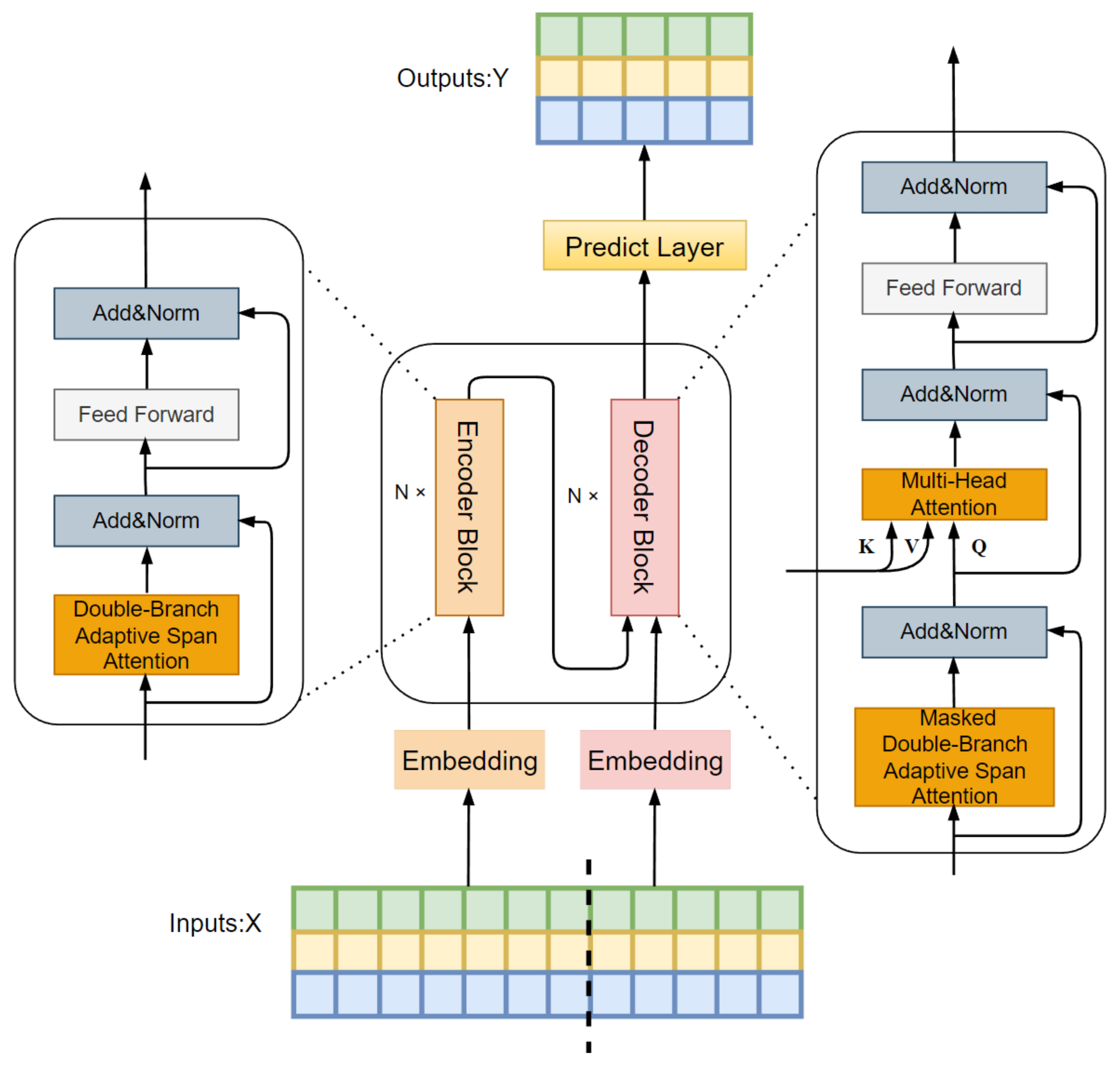
In the DBASformer architecture, the encoder and decoder follow the canonical Transformer architecture [31]. The encoder is composed of multiple encoder blocks, each consisting of an attention layer and Feedforward Networks (FFNs). In the attention layer, we replace the traditional global attention mechanism with a double-branch adaptive span attention mechanism. Similarly, the decoder is made up of multiple decoder blocks. Each module includes a masked attention layer, a multihead attention layer, and FNNs. In the masked attention layer, we employ a masked dual-branch adaptive span attention mechanism instead of the original masked global attention. The multihead attention layer computes cross-attention to integrate information from both the encoder and decoder. This involves using the encoder’s output as the key and value, and the decoder’s previous output as the query. The prediction layer generates predicted values based on potential representations acquired through training. Figure 1 illustrates the framework diagram of DBASformer. The proposed attention mechanism comprises two branches for extracting temporal and dimensional features, respectively. The first branch conducts adaptive span attention across the time steps within the same dimension, while the second branch conducts adaptive span attention across multiple dimensions. The final attention score is calculated through the weighted summation of the outputs from the two branches.
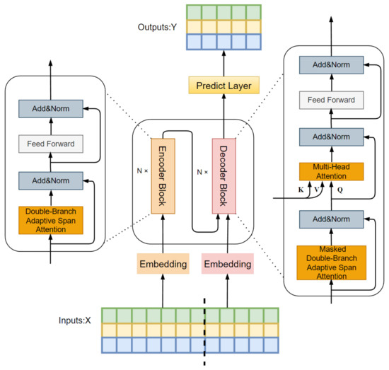
Figure 1.
Frameworkof DBASformer.
Inspired by Crossformer [32], we segment the input sequence into a series of parts before embedding them as vectors. The data in each dimension are combined into segments of length and then embedded via segments into a token independently:
where , , , is the data at t position in dimension d sequence, is the segment at i position in dimension d with length , and L is the length of the input sequence.
In sequential data, adjacent data points have similar attention weights, thereby offering limited information regarding the value at a singular time step. This segmented embedding primes the model for capturing multivariate time series relationships in subsequent steps by furnishing a more structured representation of the model inputs, reflecting the correlation and enhancing the computational efficiency of the model.
3.2. Adaptive Span Attention
In previous trajectory sequence prediction scenarios employing a canonical attention mechanism, predicting all future time steps involved computing a weighted sum of the entire historical sequence. This canonical cross-attention mechanism endeavors to compute all possible key-value pairs. However, utilizing information from the entire sequence does not necessarily improve prediction accuracy, but rather increases computational complexity. This holds particularly true when dealing with time series data characterized by evolving feature distributions, among which trajectory sequences are included.
Traditional global attention has time and memory complexity, where n is the length of the sequence, severely constraining the length of the input sequence. Despite the use of segmented embedding, global attention demonstrates a notably low efficiency. Relying solely on local attention can cause the loss of valuable information from distant positions. Consequently, existing attention mechanisms exhibit inflexibility.
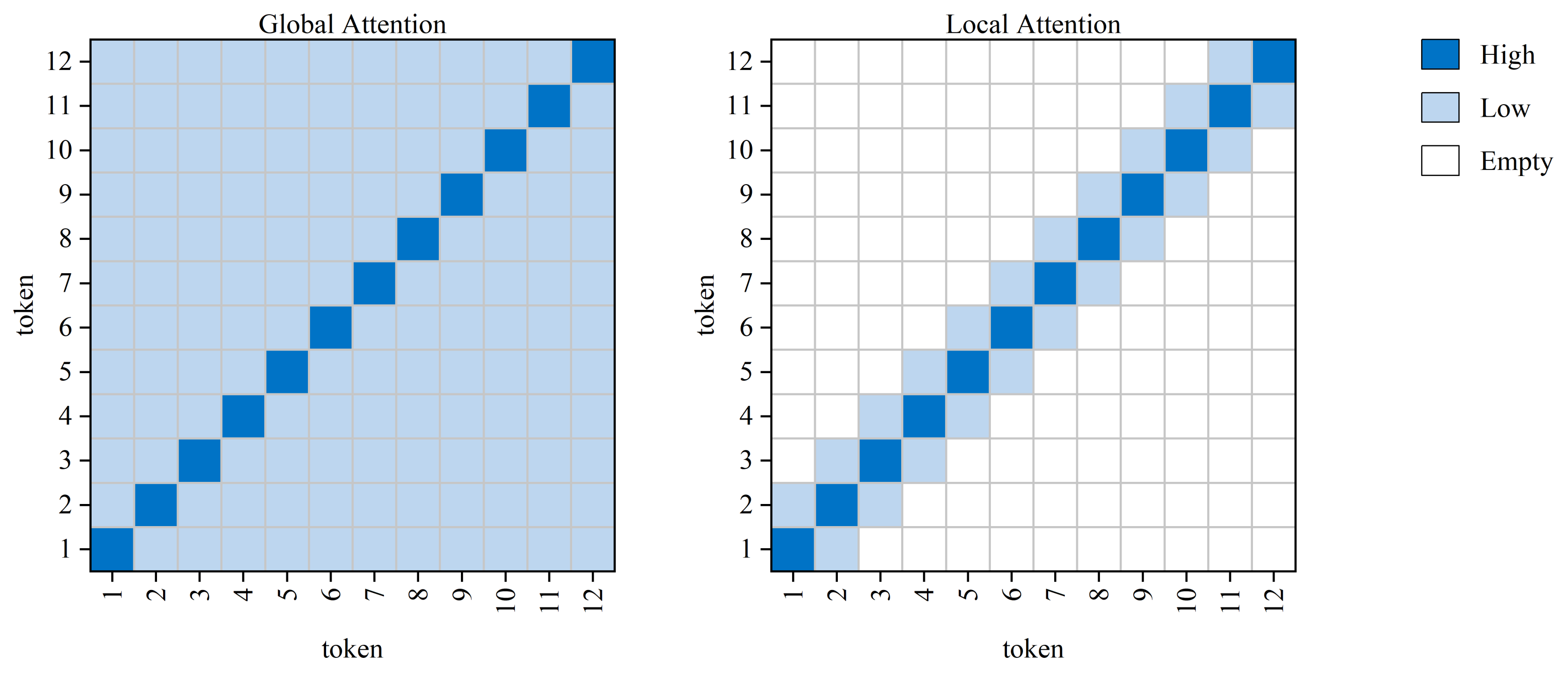
Figure 2 illustrates two attention patterns. In the global attention pattern, each token computes attention with every other token. In the local attention pattern, each token only computes attention with its neighboring tokens.

Figure 2.
Two attention patterns are depicted: white areas signify empty attention, light blue areas represent low attention, and dark blue indicates high attention from each token to itself.
The attention layer is a key part of the Transformer network. For the attention head, for a token located at position t within the sequence, the similarity with other tokens within a historical range of w is calculated:
where is the vector of the current token, is the vector transpose, and is the vectors of the other tokens in the range w. and are the weight matrices of the key and query, respectively.
Subsequently, a softmax function is applied to these attention scores to derive the resulting attention weights:
where is the natural exponential function and is used for nonlinear transformation.
In DBASformer, the model adopts a multilayer structure. To enhance the model’s flexibility in capturing local information in series, this paper proposes an adaptive mechanism to regulate the attention span, enabling the attention heads to autonomously learn the minimal required span. Specifically, a masking function with learnable parameters is added to restrict the attention span during the computation of attention weights. In this masking function, the hard masking probability is replaced with a soft masking probability that aims to interpolate the distance between the history token and the target between . Moreover, the adaptive span S is a trainable parameter in the masking function, and different mask matrices can be generated according to the varying span S, thereby assigning zero probability to irrelevant information. Throughout model training, the span S is automatically fine-tuned by the optimizer to minimize the loss function. Specifically, the adaptive span S does not increase but only decreases by 1 segment length unit at a time.
The masking function is defined as a piecewise function, wherein the soft mask component is specified as a sigmoid-like function. The function is expressed by the following formula:
where is the distance between position r and the current position t in the sequence, and S is the adaptive span of attention.
Then, compute the attention weights based on an adaptive span:
where s is the attention span and is the masking probability at position p.
Finally, the attention weight outputs from different heads are concatenated for the next computation.
Traditional attention mechanisms compute attention scores over a fixed range, but certain information within this range may lack relevance. Adaptive span attention improves the flexibility of the attention mechanism through a novel masking function. Following computing the attention scores within the original range, the model automatically retains a certain range of attention scores for computing attention weights during the training phase. This process aims to maximize the retention of useful information while mitigating the influence of irrelevant or noisy data. This dynamic methodology enables the model to capture critical features with greater precision.
3.3. Double-Branch Attention
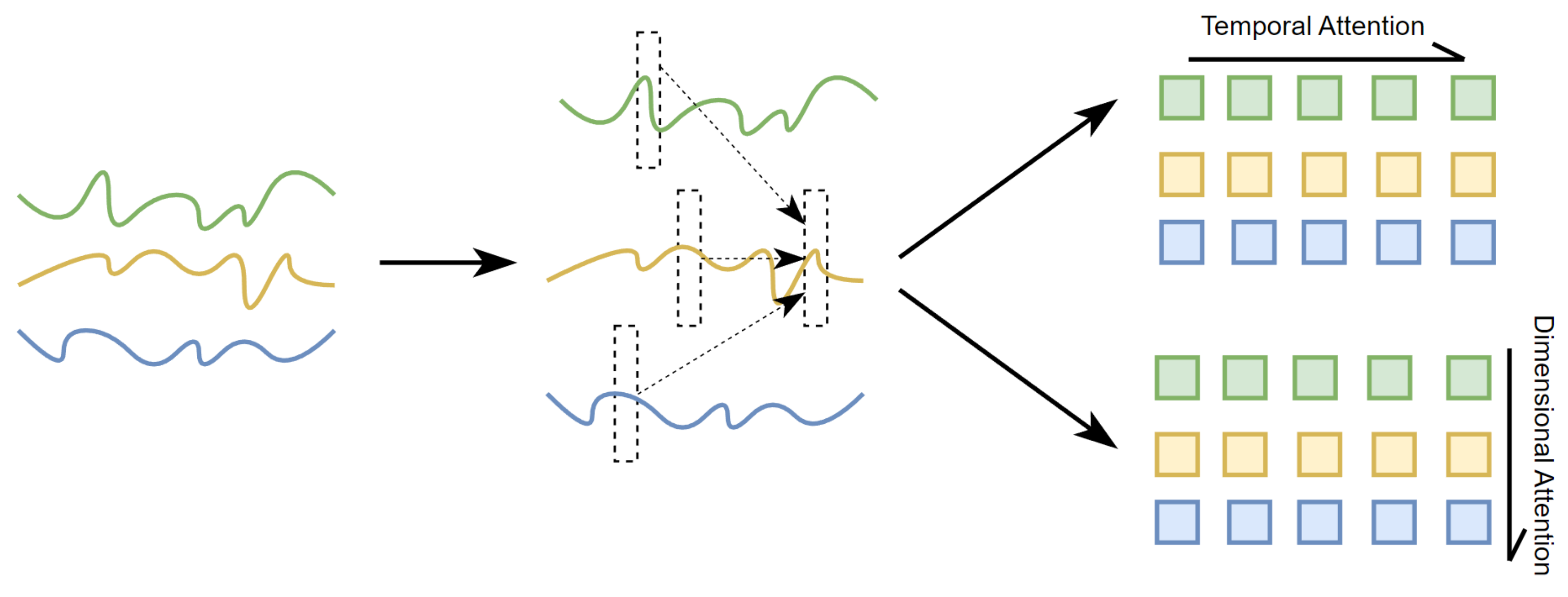
Drift trajectories are the result of a combination of influences. In the case of drift data featuring multivariate variables, numerous variables exhibit temporal interdependence or correlation. It is worth noting that neighboring trajectory points exhibit higher correlations during temporal changes, and alterations in the characteristics of other variables can improve the accuracy of predicting the current trajectory point. In summary, univariate sequences display temporal dependence, whereas multivariate variables demonstrate dimensional dependence. Building upon this observation, double-branch attention is introduced, which is a pivotal difference from existing methods. As illustrated in Figure 3, the two branches operate concurrently, with one capturing the cross-time dependency of sequences while the other focuses on the cross-dimension dependency between different variables.
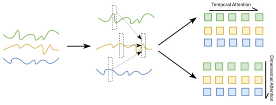
Figure 3.
Double-branch attention mechanism: yellow represents the drift trajectory, green and blue represent the variables that affect the drift.
Temporal attention module: Time series data are usually considered to be generated from a conditional distribution of historical values, wherein adjacent data points have similar values. Thus, utilizing the dependencies between periods in the same dimension can help in calculating the attention weight of tokens. However, employing the global attention mechanism directly on the embedding vector will result in a secondary computational complexity ( memory usage) when computing the attention scores between each pair of segments.
The temporal attention module is based on adaptive span attention, which considers the correlation of sequence data during temporal evolution. Meanwhile, adaptive span attention permits the computation of similarity solely between tokens within the attention span. Calculating the attention score by applying the following formula:
where is the vector of tokens at the current position and is the vector of other tokens in the same dimension in the span.
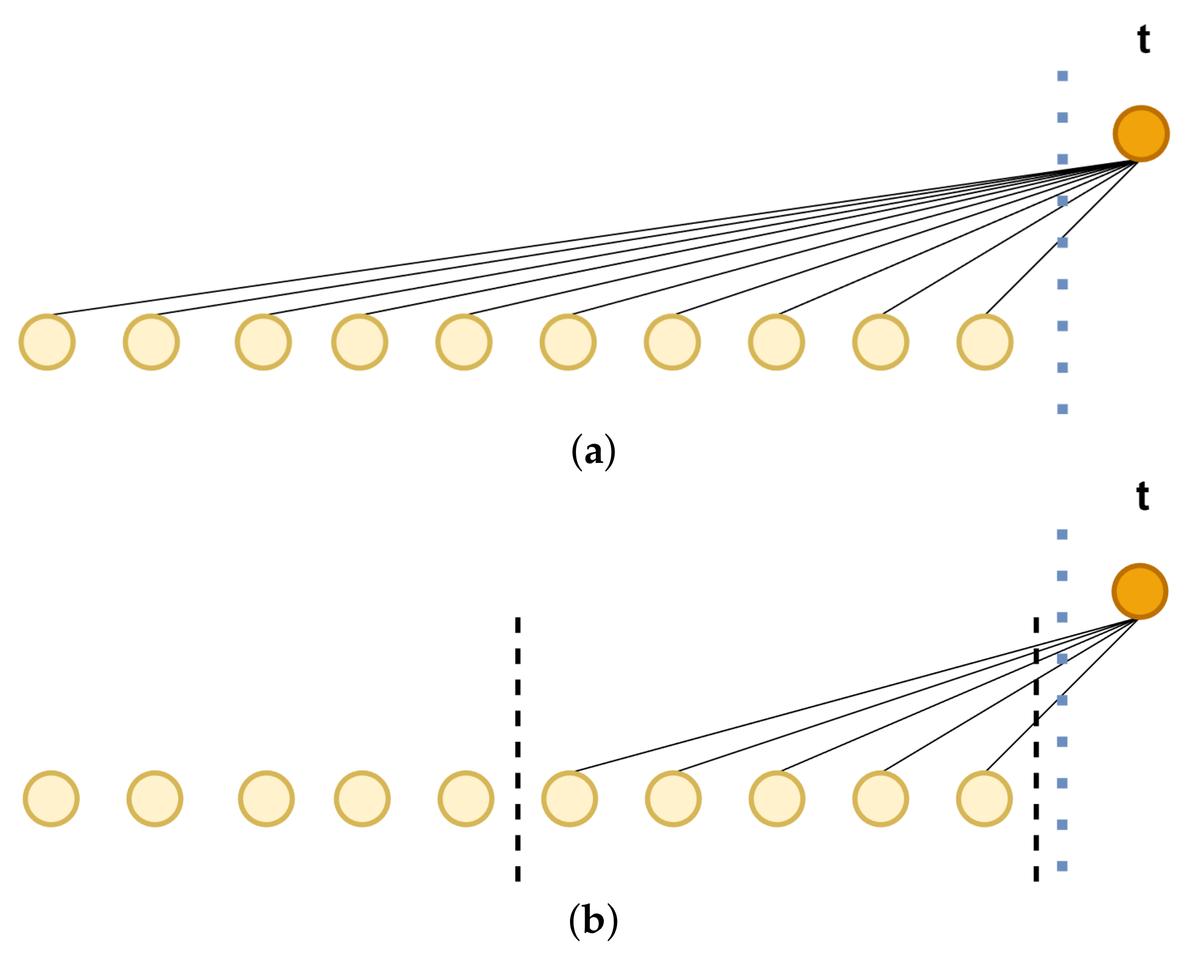
Unlike global attention, the temporal attention module focuses on localized regions in the same dimension (Figure 4), and the range of attention is determined by the adaptive attention span. The temporal attention module measures the importance of data points by relative time during modeling sequences, thereby effectively capturing the temporal relevance of sequences and rationally allocating attention weights.
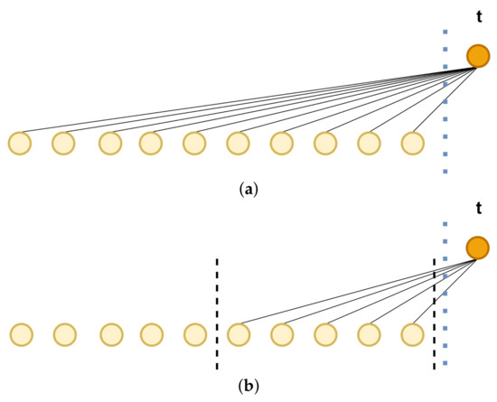
Figure 4.
Forms of temporal attention: (a) high span and (b) low span, dashed line represents the range of attention, yellow indicates the historical token, and orange represents the current position within the token.
Dimensional attention module: Previous studies [33,34,35,36] have demonstrated the correlation among sequences of different variables within the same process during changes, which serves as a foundation for predicting future periods. Due to variations in the degrees of redundancy or potential conflicts within different sequences, it is unwise to directly splice and fuse the multidimensional information. The existence of complex relationships between multiple variables cannot be ignored in the task of predicting drift trajectories.
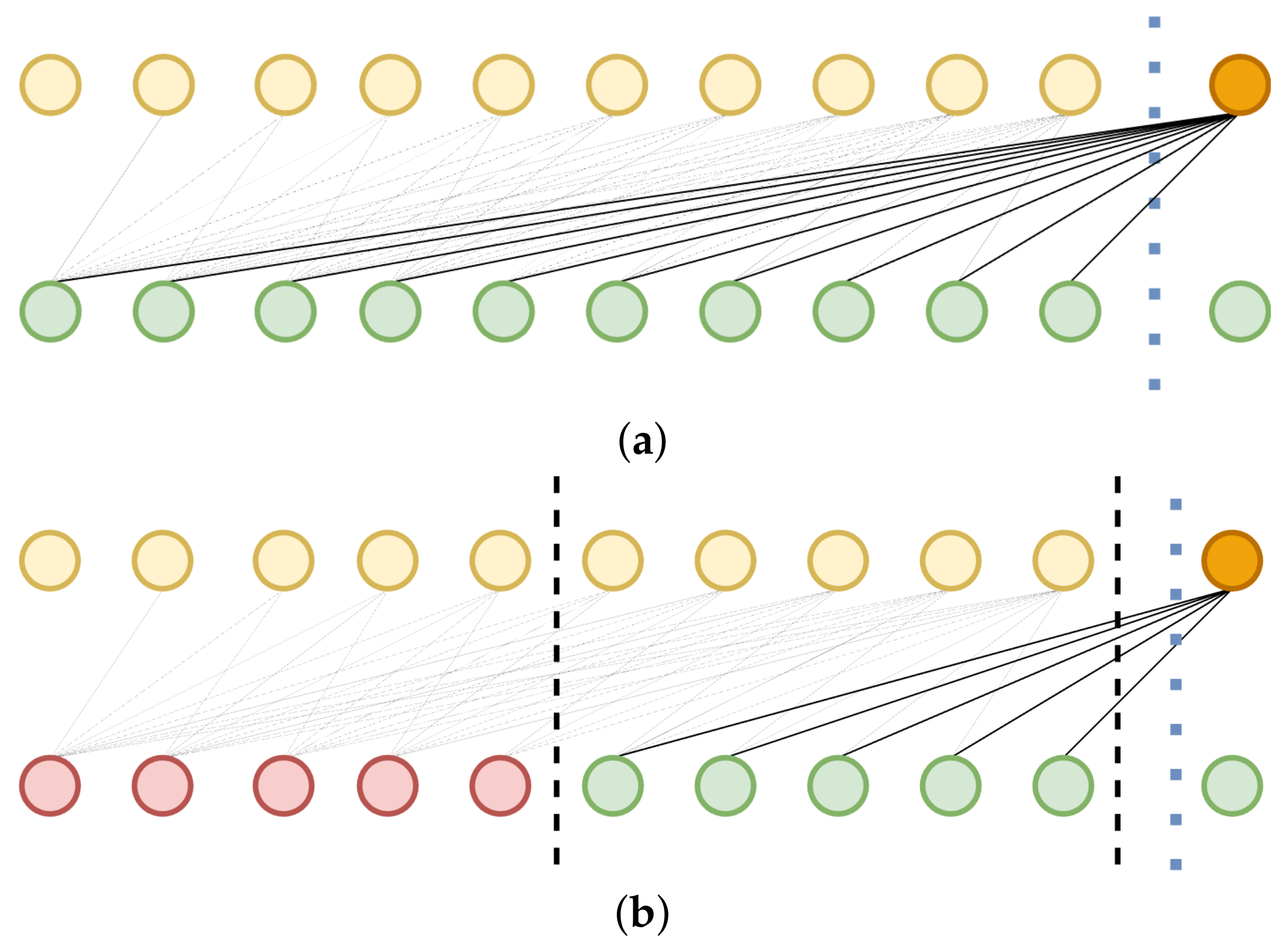
The proposed double-branch attention structure incorporates dimensional attention branching to thoroughly leverage the interdependencies among different variables. When conducting dimensional attention, adaptive span attention is employed on the vector , wherein the range of targets is dictated by the attention span. Notably, this attention span is still divided according to the time-step relationship (Figure 5) to compute the similarity between tokens in different dimensions:
where , are different dimensions, and denotes other tokens with different dimensions than the one in which is located.

Figure 5.
Forms of dimensional attention: (a) high span and (b) low span, dashed line represents the range of attention, yellow indicates historical token in the same dimension as orange, green represents token from another dimension, red indicates token that is not included in the attention calculation.
Lastly, the weighted sum of and is calculated:
where and are the weights of the two forms of attention, which are updated following the model learning.
Then, compute the attention weights based on the adaptive span:
The dimensional attention module calculates the correlation among different dimensional tokens, thereby improving the model’s capability to extract multidimensional features. In contrast to previous methods, the double-branch attention mechanism distinguishes between temporal and dimensional correlations during attention weight computation. Tokens within the same dimension are assigned higher weights for temporal correlation, while tokens across different dimensions are given higher weights for dimensional correlation. The weighted summation approach can combine temporal and dimensional attention scores to utilize information from both in a balanced way, resulting in a more comprehensive and accurate attention score.
4. Experiments
This section comprises the following components: dataset preparation, experimental hyperparameters setting, selection of evaluation metrics, experiments of the proposed method, and comparison experiments. The drift trajectory dataset and the underwater vehicle dataset presented in this section are grounded in realistic scenarios. Furthermore, this section presents the performance of DBASformer on these two datasets, along with comparative results against existing trajectory-prediction methods, aiming to demonstrate that the proposed method can improve prediction accuracy.
4.1. Dataset Preparation
To ensure the predictive ability of the model, we fully considered the typical representatives of drifters in the ocean, ultimately opting to use the trajectories of drifting buoys and AUVs as the experimental data. The motions of buoys and AUVs are affected by the currents. The motion trajectory data encompass time, longitude, and latitude, with the experimental dataset additionally incorporating current flow rate information. The drift trajectories of buoys were acquired from the Argo buoy metadata available at the Global Data Assembly Center (GDAC) [37]. Argo buoys are deployed at a depth of around 1000 m. The AUVs dataset was sourced from the BCO-DMO website [38], and the data of AUVs originate from their drifting processes at depths ranging from 1 to 30 m. The dataset for the buoys comprises Argo buoy trajectory data spanning from January 2004 to June 2023. The raw dataset primarily includes variables such as the buoy’s ID, timestamp, longitude, latitude, current flow rate, and Quality Control (QC) flags. Multiple trajectory sequences can be distinguished based on the ID. Specifically, We select data with a time interval of 10 min, and QC flags are categorized into metadata and interpolation depending on the type of data. The quality of buoy trajectory sequences is assessed based on the QC flags, and sequences ranked in the top 70% are chosen as the experimental data. As shown in Table 1, the experimental data includes four parameters: time, latitude, longitude, and ocean current velocity.

Table 1.
Parameters of buoy data.
Regarding the underwater vehicle dataset, we established a time interval of 3 min in data and conducted data cleaning to remove redundant values and outliers. The region of interest is a rectangle from (36.8338, −121.828) to (36.7837, −121.888). Linear interpolation was employed to impute missing data at certain time points, ensuring the preservation of valuable information to the fullest extent possible. Similarly, the experimental data of AUVs include four parameters: time, latitude, longitude, and current velocity.
The dataset is indexed in chronological order and divided into training, validation, and test sets in the ratio of 8:1:1. This division ensures that the models are trained on a substantial portion of the data while also being validated and tested on unseen samples, thereby maintaining the integrity of the evaluation process.
4.2. Experimental Hyperparameters Setting
The DBASformer model proposed in this study is implemented using PyTorch. In the primary experiments, we employ the DBASformer architecture with four encoder blocks and decoder blocks. The input lengths are selected from {64, 128, 192, 256, 320} based on the varying time intervals of the data. The time interval of buoy trajectory data is 10 min, and the length L of the input buoy historical trajectory sequence is set to 128. The time length of input buoy data is 1280 min. As the time interval of AUV trajectory data is 3 min, the length L of the input AUV historical trajectory sequence is set to 256. The time length of input AUV data is 768 min. Their prediction length is set to 32, and longer prediction lengths reduce prediction accuracy. So, we predict the buoy drift trajectory for the next 320 min and the AUV drift trajectory for the next 96 min. The segment length is set to four. The predetermined attention span size S is set to 16. The Adam optimizer is utilized for training DBASformer, with the initial learning rate selected from {, , , } and updated using the Cosine Annealing Scheme throughout the training procedure. The total number of epochs is configured as 20, and this value can be adjusted accordingly based on the training speed.
Table 2 illustrates the computer configurations necessary for conducting the experiments. It is ensured that all experiments in this paper are conducted under identical hardware and software environments to maintain comparability and fairness.
Table 2.
Experimental environment.
4.3. Evaluation Indicators and Comparative Models
Prediction accuracy is evaluated by computing the Mean Square Error (MSE) and Mean Absolute Error (MAE) between the predicted trajectory data and the actual trajectory data :
This paper compares DBASformer with five trajectory-prediction approaches. We evaluated the performance of the original model from the reference paper on our synthetic dataset, adopting the hyperparameters recommended in the original paper, such as the number of layers and batch size, to approximate the model’s optimal performance. All models have the same input length and output length. The following is a brief description of the compared models:
BiLSTM [6]: This model comprises two bidirectional LSTM layers, totaling four LSTM units. The hidden layer includes an LSTM layer. The input vector contains all the features, propagated through the BiLSTM layer to obtain the output.
CNN-LSTM [7]: This model integrates CNN and LSTM through a tandem structure. The CNN module contains convolutional, BatchNorm, Dropout, Extension, and fully connected layers, while the LSTM module contains two LSTM layers.
RGA [23]: This model contains a ResNet layer, a fully connected layer, two GRU layers, an attention layer, and an output layer. Notably, a 2D convolutional layer forms the core of the residual block, while the hidden state from the second GRU layer is utilized as the input to the attention mechanism.
TrAISformer [10]: This model adopts a Transformer architecture similar to GPT. The Transformer network consists of a series of stacked attention layers, with each layer functioning as an autoregressive model and employing a dot-product multihead attention mechanism.
TRFM-LS [11]: compared with the traditional Transformer structure, the output after the LSTM processing sequence is added as the input of the decoder.
4.4. Experimental Results
To validate the accuracy of the predicted trajectories generated by DBASformer, trajectory data from buoys and AUVs were used to train and test the network model. By comparing the model prediction results to the actual trajectories, accuracy is evaluated based on proximity to the real trajectories. The experimental results show that DBASformer achieves good prediction results in trajectory sequence prediction and exhibits practical efficacy. Moreover, compared to alternative models, DBASformer achieves a higher prediction accuracy. Table 3 presents the MSE and MAE of DBASformer’s prediction results along with those of each comparative model on the synthetic dataset.
Table 3.
Errors in predicting buoy and AUV trajectories by different models.
DBASformer effectively improves the prediction accuracy of the trajectory sequence. As depicted in Table 3, DBASformer exhibits smaller error values compared to all comparison models. The MSE for predicting the buoy trajectory is 0.1539, with an MAE of 0.1151. The MSE of predicting the AUV trajectories is 0.1708, with an MAE of 0.1415.
For a clearer and more intuitive display of the prediction results, we present plots of predicted and true values for the same period. The trajectory curves constitute a crucial foundation for evaluating the quality of the predictions. Before generating the curve, we perform Min–Max Normalization for the predicted and true values. This visual representation enables a more intuitive assessment of the prediction accuracy.
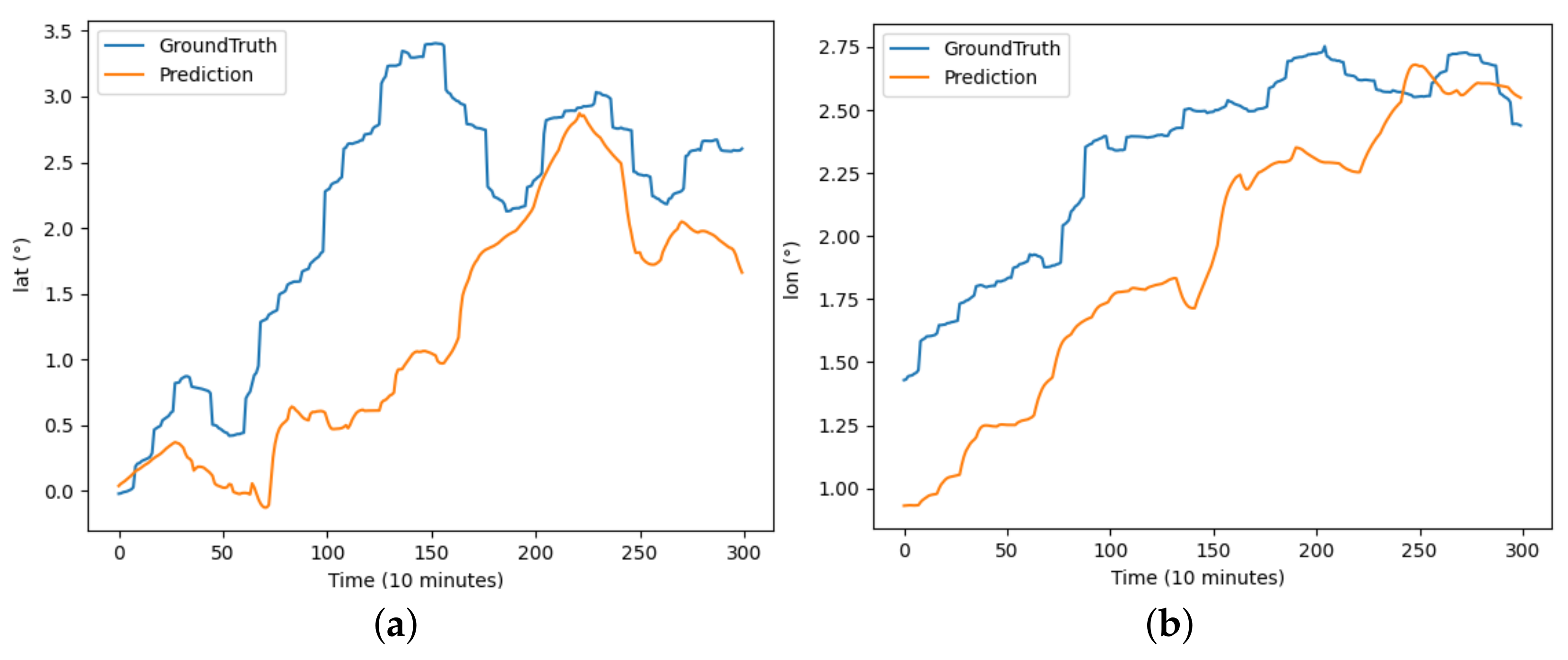
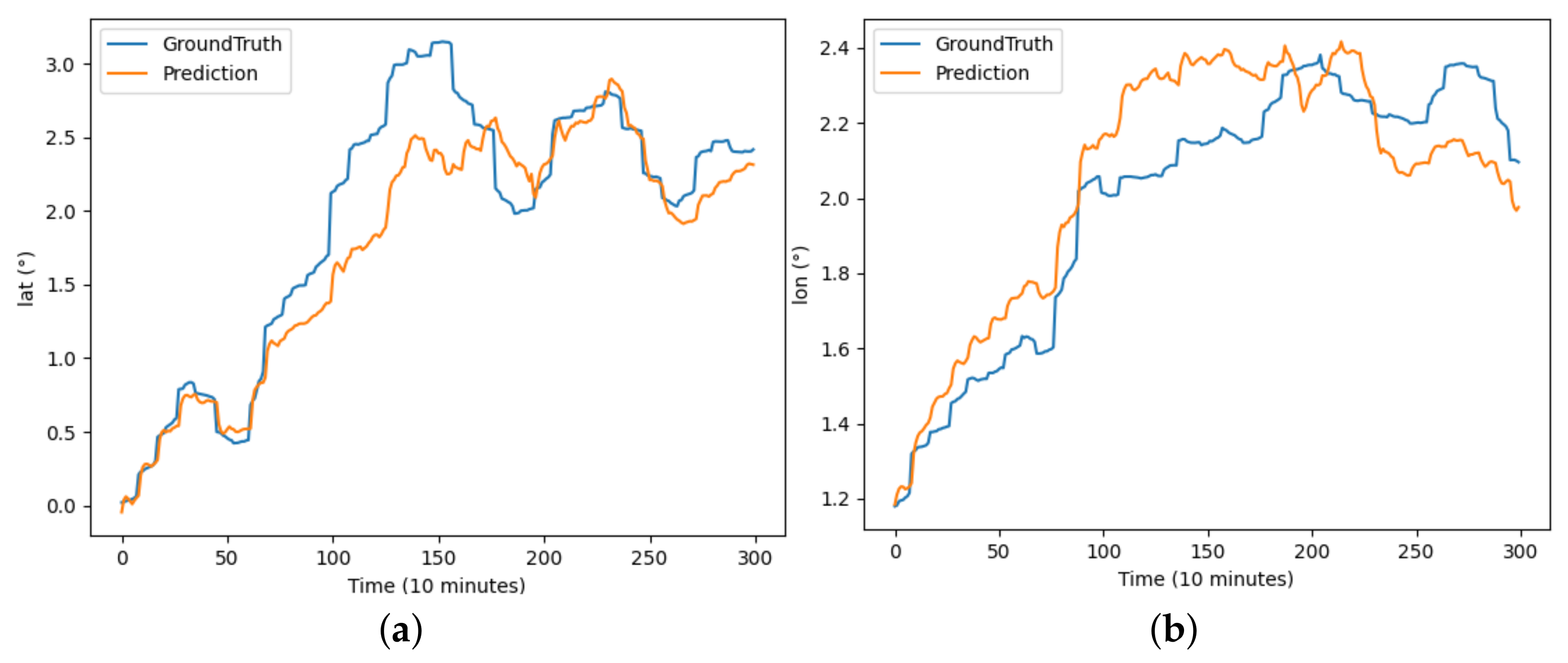
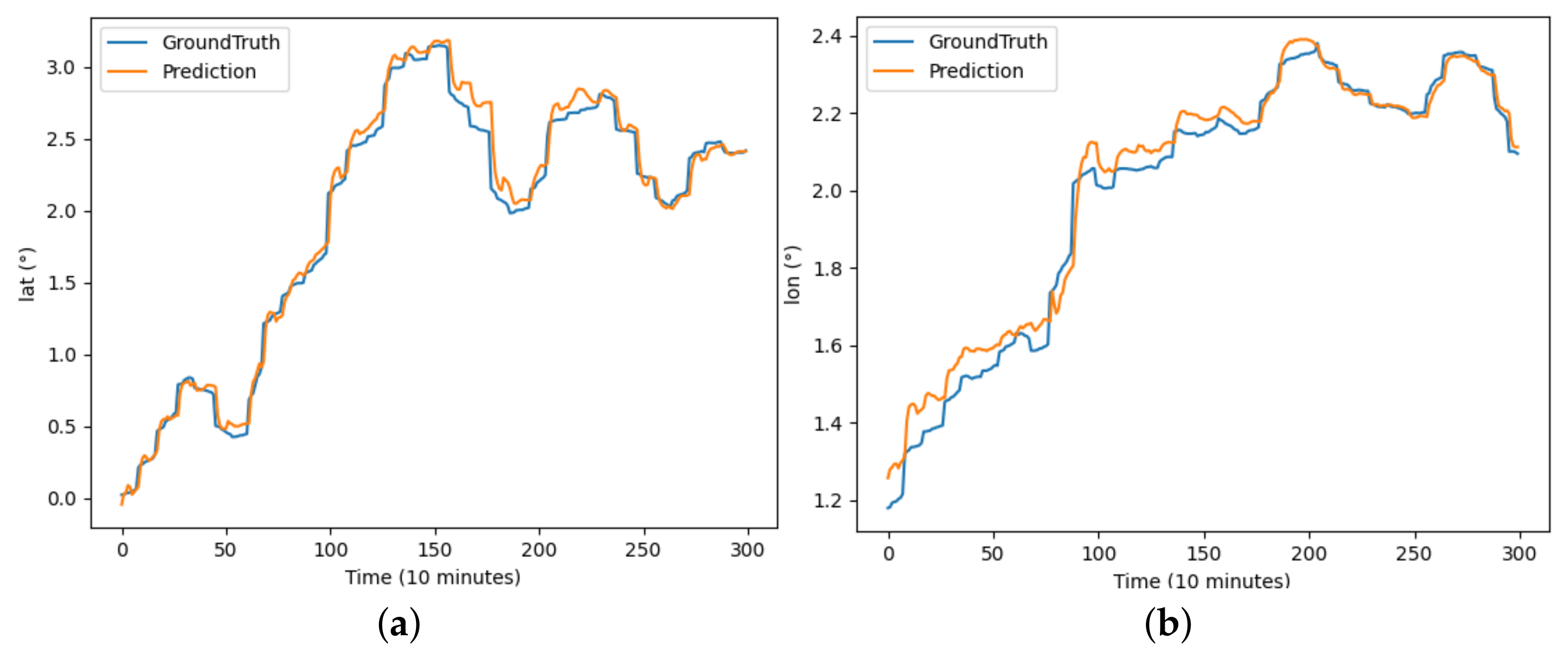
The performance of each model on the buoy trajectory dataset is illustrated in Figure 6, Figure 7, Figure 8, Figure 9, Figure 10 and Figure 11, where DBASformer has the best curve fit between the true and predicted values. Based on these results, the poor performance of the other models is due to the complexity of the dataset, which includes multiple variables. Some models may struggle to capture multidimensional features effectively, thus reducing the predictive efficacy. This observation reflects the capability of the trajectory-prediction method proposed in this study to address this challenge.
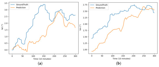
Figure 6.
The results of the BiLSTM model predicting latitude and longitude for buoy trajectory: (a) illustrates the prediction of latitude over the period and (b) illustrates the prediction of longitude over the period.

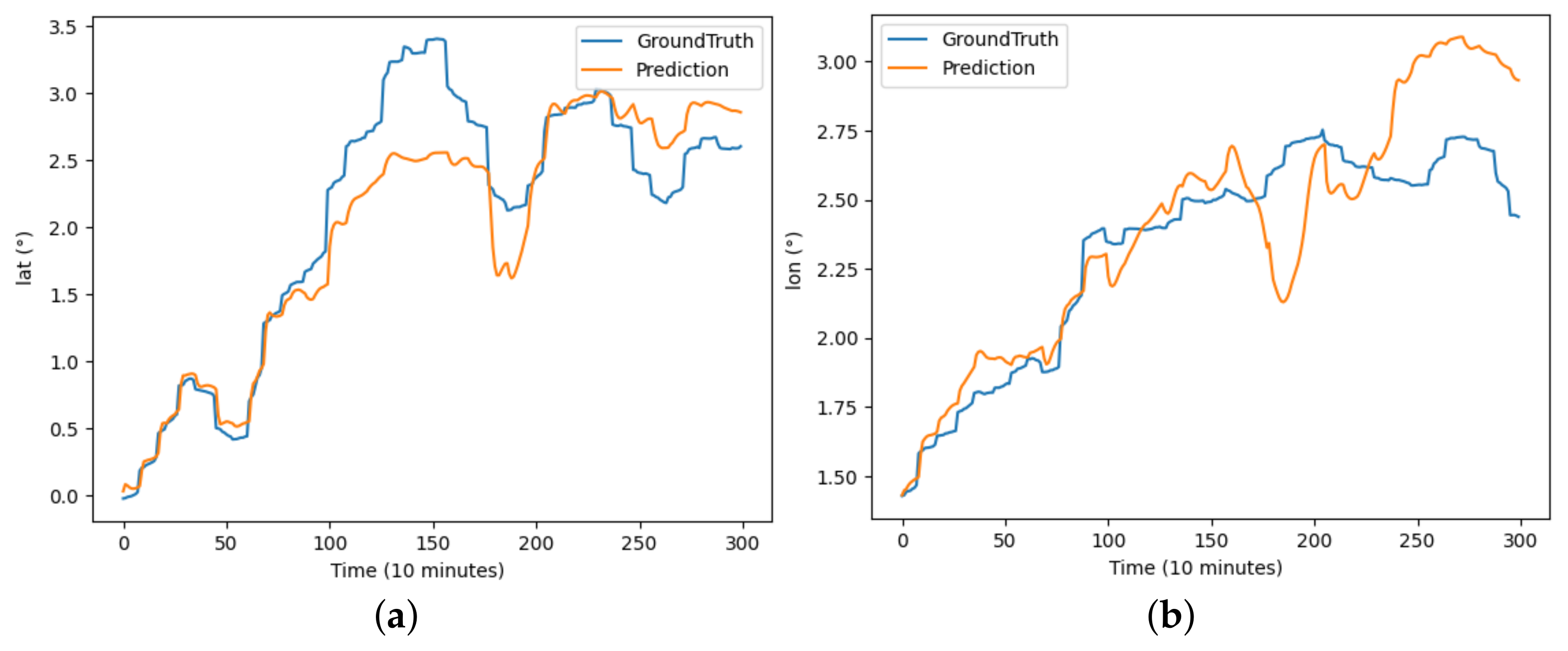
Figure 7.
The results of the CNN-LSTM model predicting latitude and longitude for buoy trajectory: (a) illustrates the prediction of latitude over the period and (b) illustrates the prediction of longitude over the period.
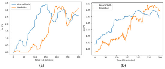
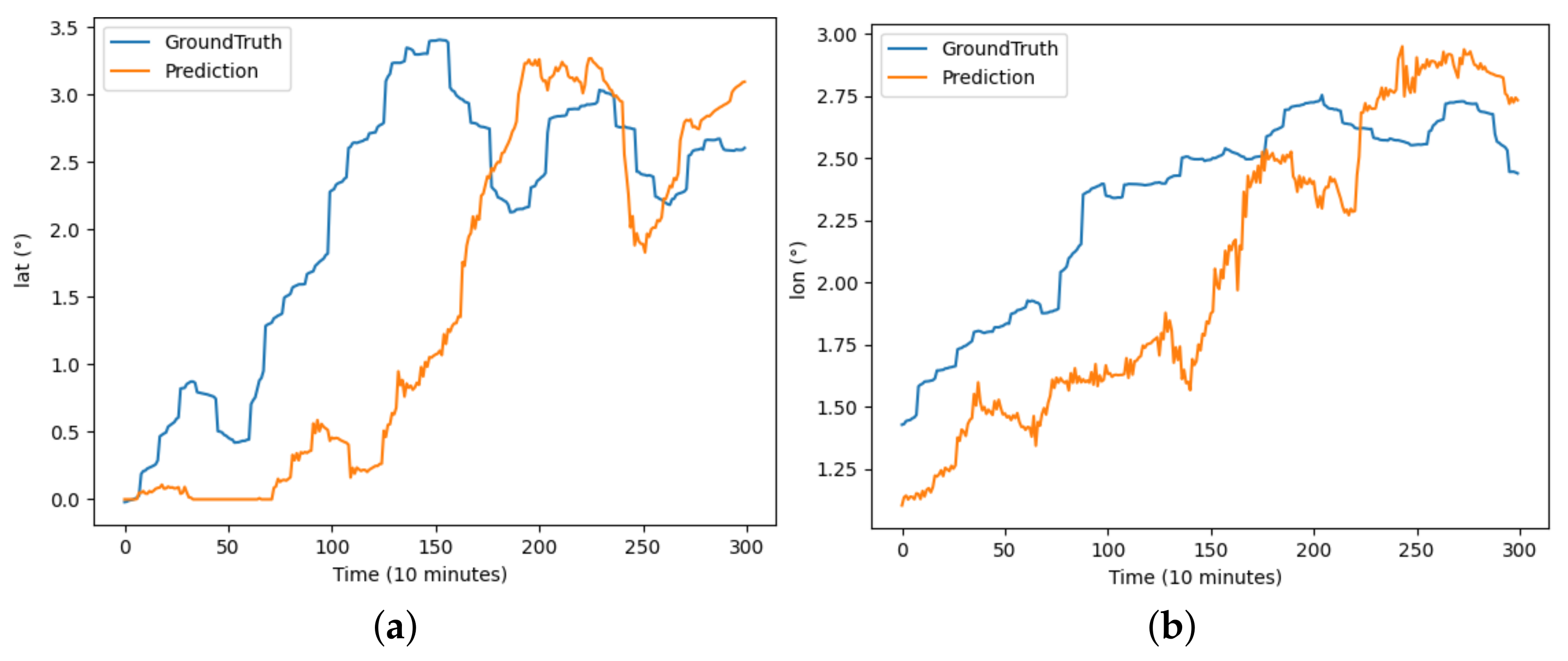
Figure 8.
The results of the RGA model predicting latitude and longitude for buoy trajectory: (a) illustrates the prediction of latitude over the period and (b) illustrates the prediction of longitude over the period.
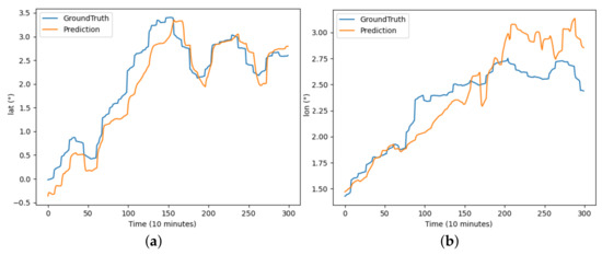
Figure 9.
The results of the TrAISformer model predicting latitude and longitude for buoy trajectory: (a) illustrates the prediction of latitude over the period and (b) illustrates the prediction of longitude over the period.
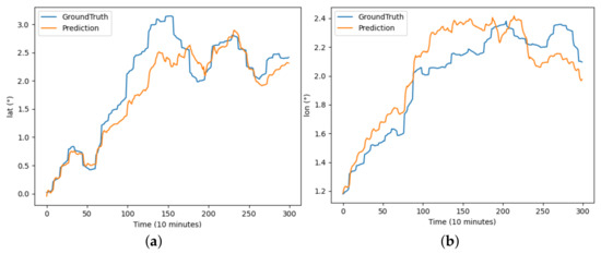
Figure 10.
The results of the TRFM-LS model predicting latitude and longitude for buoy trajectory: (a) illustrates the prediction of latitude over the period and (b) illustrates the prediction of longitude over the period.
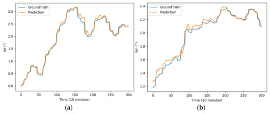
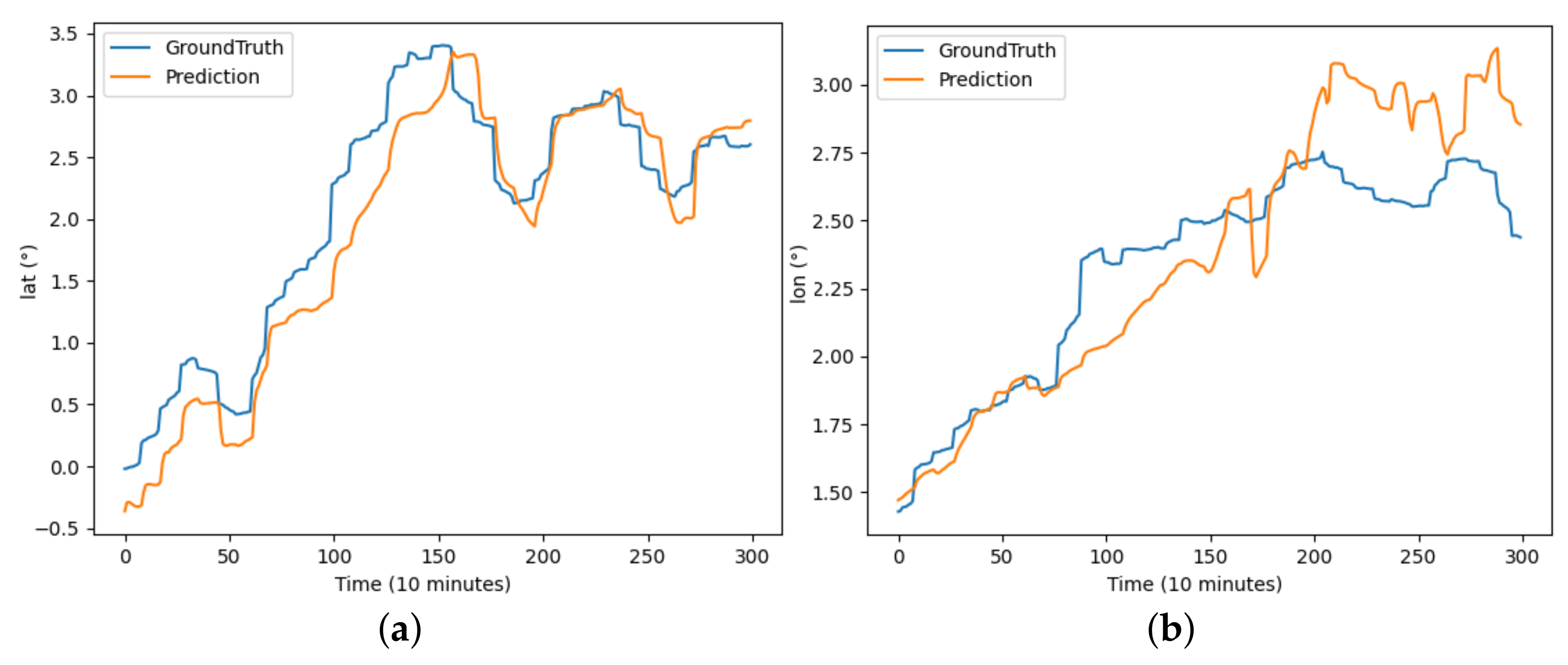
Figure 11.
The results of the DBASformer model predicting latitude and longitude for buoy trajectory: (a) illustrates the prediction of latitude over the period and (b) illustrates the prediction of longitude over the period.
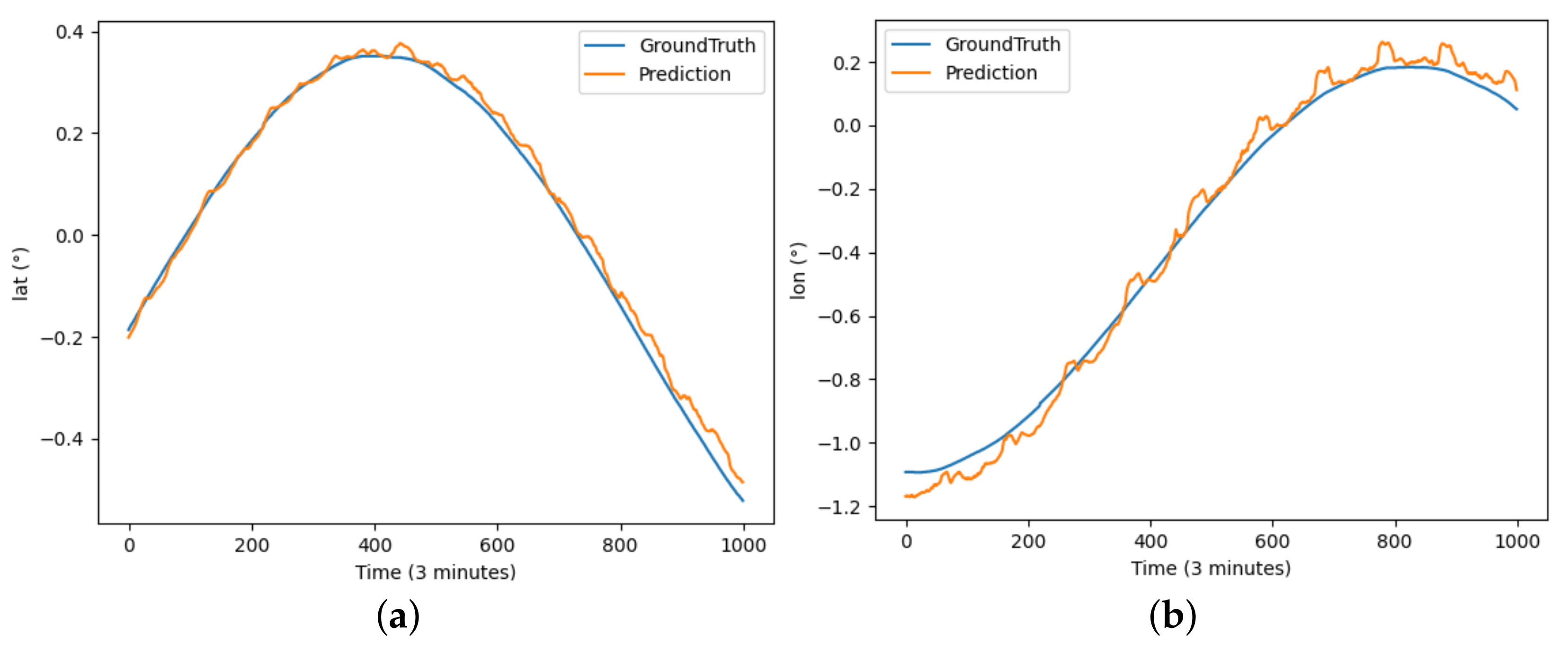
Furthermore, DBASformer was utilized to predict AUV trajectories in order to evaluate its performance across another dataset.
As depicted in Figure 12, DBASformer also captures the trajectory trend of the AUV data.
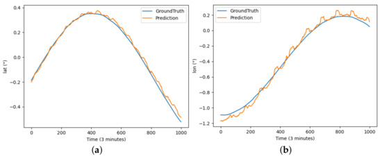
Figure 12.
The results of DBASformer model predicting latitude and longitude for AUV trajectory: (a) illustrates the prediction of latitude over the period and (b) illustrates the prediction of longitude over the period.
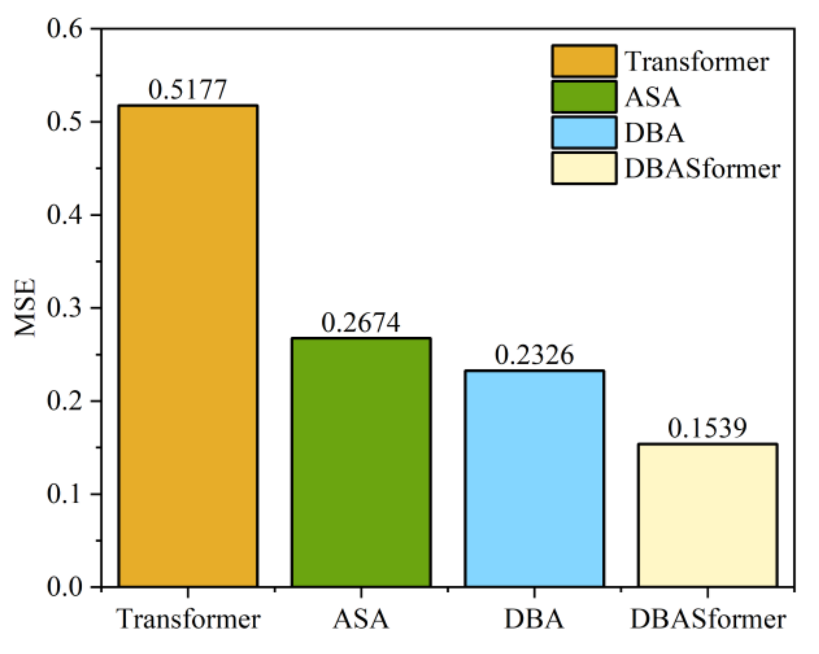
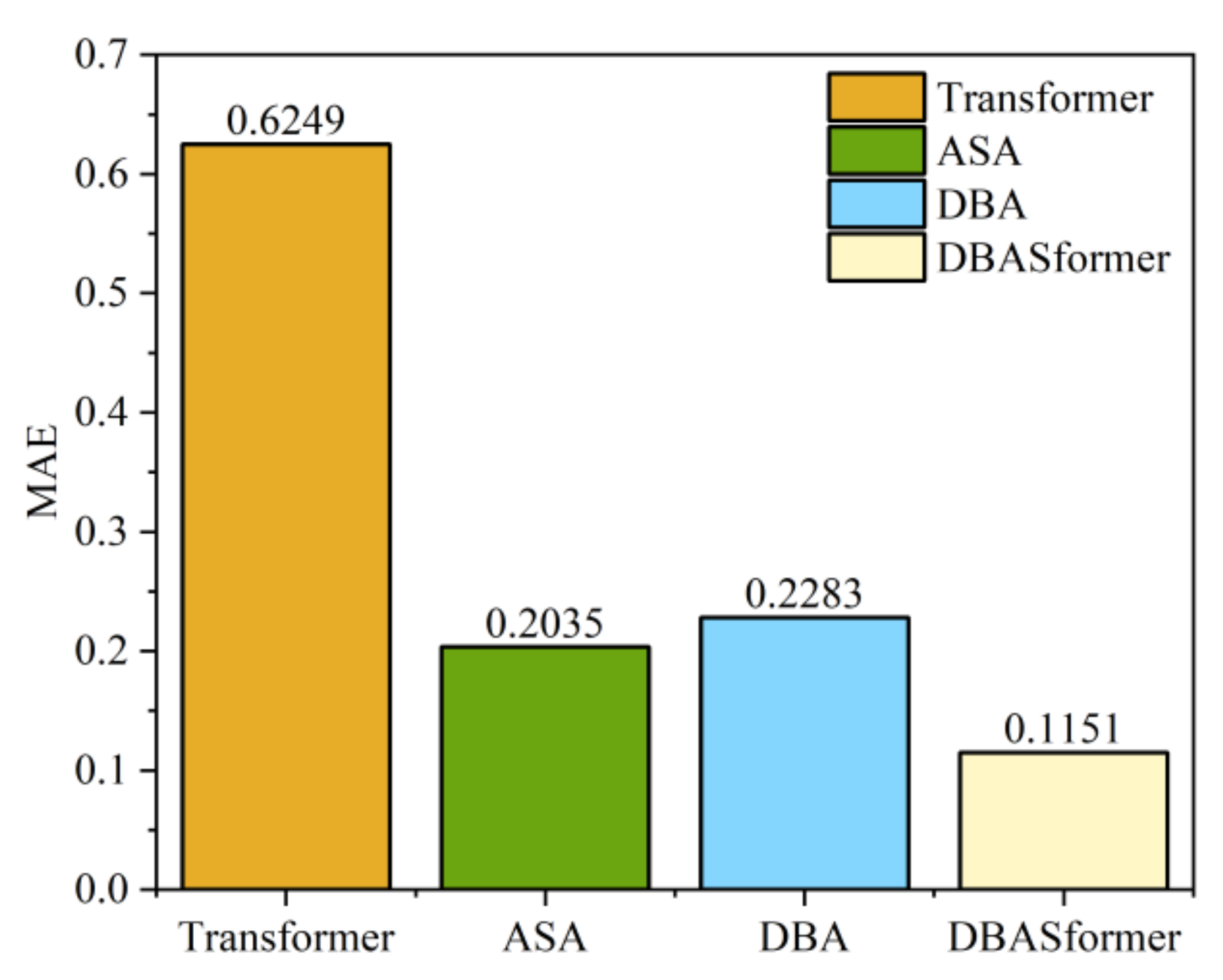
In the proposed method, comprising adaptive span attention (ASA) and double-branch attention (DBA), we used the Transformer as a baseline to evaluate their performance. DBASformer represents the comprehensive model encompassing both ASA and DBA. Figure 13 and Figure 14 present the MSE and MAE of the predictive outcomes of models incorporating various components, respectively. The prediction errors of models incorporating components are consistently lower than those of the Transformer baseline. Specifically, the MSE stands at 0.5177 for the Transformer, 0.2674 for ASA alone, and 0.2326 for DBA alone. DBASformer contains both ASA and DBA, with an MSE of 0.1539.
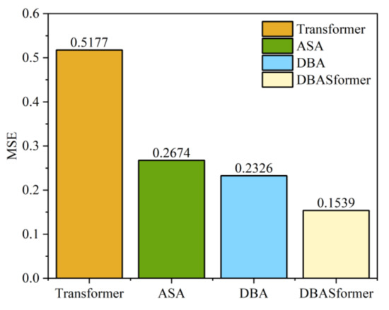
Figure 13.
MSE of prediction on the buoy dataset.

Figure 14.
MAE of prediction on the buoy dataset.
The results of the version with DBA are significantly better than the baseline model, which may be because the traditional Transformer inputs the data as 1D, ignoring cross-dimensional dependencies in the sequence. This suggests that our addition of attention branching can capture correlations between different variables.
Replacing ASA within the Transformer framework leads to a substantial reduction in prediction error. Unlike the fixed-width traditional attention mechanism, ASA offers enhanced flexibility in accurately distributing attention weights based on the data, thus justifying the incorporation of a learnable attention span for capturing pivotal features. The integration of ASA and DBA yields the lowest prediction error, highlighting the efficacy of the proposed approach in managing multivariate sequential data.
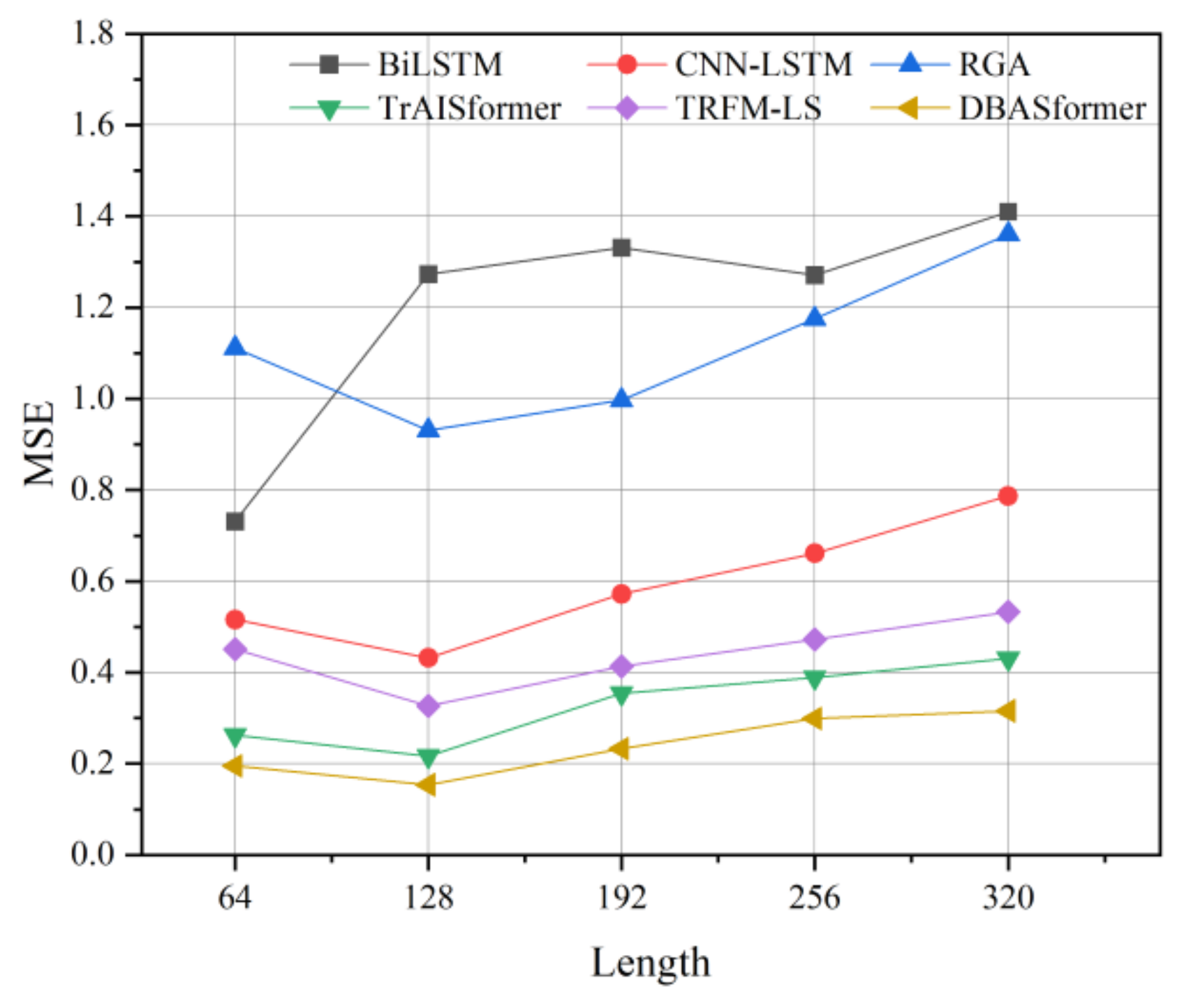
The effect of hyperparameter input length on the buoy dataset was evaluated. In Figure 15, we prolong the segment length from 64 to 320 and evaluate the MSE with different models. For most models, the best results are obtained when the input length is 128. Additionally, prolonging the input length from 128 to 320 causes the MSE to increase.
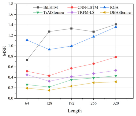
Figure 15.
MSE with different input lengths on the buoy dataset.
5. Conclusions
This study presents a novel model, named DBASfomer, designed for predicting the trajectory of underwater drifters in the ocean. DBASfome captures the changing characteristics of trajectories and currents, utilizing them to forecast future drift trajectories, consequently leading to a substantial reduction in prediction errors. The proposed adaptive span attention mechanism, along with the double-branch attention structure, exhibits the capability to learn complex dependencies in multivariate drift trajectory sequences. Buoy datasets containing trajectory and current velocity information, alongside AUV datasets, are collated from raw real data and employed to evaluate the model. The experimental results show that the prediction accuracy of DBASformer is better than the existing trajectory-prediction methods. The MSE and MAE for predicting buoy trajectory data stand at 0.1539 and 0.1151, respectively, considerably lower than comparative models. Furthermore, the model performs well on the underwater vehicle dataset, achieving MSE and MAE values of 0.1708 and 0.1415, respectively. To validate the efficacy of all components in the proposed method, the prediction errors of DBASformer are compared with the Transformer, ASA only, and DBA only. The results show that the prediction errors of the models containing components are all lower than the Transformer. In the future, we will optimize the model for various drift motion patterns, introduce more variables to predict drift trajectories, and increase the practical application value of DBASformer.
Author Contributions
Conceptualization, C.Z. and J.Z. (Jing Zhang); methodology, C.Z.; software, C.Z.; validation, C.Z., J.Z. (Jing Zhang) and J.Z. (Jiafu Zhao); formal analysis, C.Z.; investigation, C.Z.; resources, C.Z.; data curation, C.Z.; writing—original draft preparation, C.Z.; writing—review and editing, C.Z, J.Z. (Jing Zhang) and T.Z.; visualization, C.Z., J.Z. (Jing Zhang) and J.Z. (Jiafu Zhao); supervision, J.Z. (Jing Zhang); project administration, J.Z. (Jing Zhang) and T.Z.; funding acquisition, J.Z. (Jing Zhang). All authors have read and agreed to the published version of the manuscript.
Funding
This research was funded by (1) 2022–2025, the National Natural Science Foundation of China under grant no. 52171310; (2) 2021–2023, the National Natural Science Foundation of China under grant (youth) no. 52001039; and (3) 2022–2023, Science and Technology on Underwater Vehicle Technology Laboratory no. 2021JCJQ-SYSJJ-LB06903.
Institutional Review Board Statement
Not applicable.
Informed Consent Statement
Not applicable.
Data Availability Statement
Data available upon request from the authors. The data that support the findings of this study are available from the corresponding author (ise_zhangjing@ujn.edu.cn), upon reasonable request.
Conflicts of Interest
The authors declare no conflicts of interest.
References
- Wu, J.; Cheng, L.; Chu, S. Modeling the leeway drift characteristics of persons-in-water at a sea-area scale in the seas of China. Ocean Eng. 2023, 270, 113444. [Google Scholar] [CrossRef]
- Klein, I.; Diamant, R. Dead reckoning for trajectory estimation of underwater drifters underwater currents. J. Mar. Sci. Eng. 2020, 8, 205. [Google Scholar] [CrossRef]
- Qiao, S.; Shen, D.; Wang, X.; Han, N.; Zhu, W. A self-adaptive parameter selection trajectory prediction approach via hidden Markov models. IEEE Trans. Intell. Transp. Syst. 2014, 16, 284–296. [Google Scholar] [CrossRef]
- Rabatel, M.; Rampal, P.; Carrassi, A.; Bertino, L.; Jones, C.K. Impact of rheology on probabilistic forecasts of sea ice trajectories: Application for search and rescue operations in the Arctic. Cryosphere 2018, 12, 935–953. [Google Scholar] [CrossRef]
- Zhang, X.; Cheng, L.; Zhang, F.; Wu, J.; Li, S.; Liu, J.; Chu, S.; Xia, N.; Min, K.; Zuo, X.; et al. Evaluation of multi-source forcing datasets for drift trajectory prediction using Lagrangian models in the South China Sea. Appl. Ocean Res. 2020, 104, 102395. [Google Scholar] [CrossRef]
- Yang, C.H.; Wu, C.H.; Shao, J.C.; Wang, Y.C.; Hsieh, C.M. AIS-based intelligent vessel trajectory prediction using bi-LSTM. IEEE Access 2022, 10, 24302–24315. [Google Scholar] [CrossRef]
- Li, J.; Li, W. Auv 3d trajectory prediction based on cnn-lstm. In Proceedings of the 2022 IEEE International Conference on Mechatronics and Automation (ICMA), Guilin, China, 7–10 August 2022; IEEE: Piscataway, NJ, USA, 2022; pp. 1227–1232. [Google Scholar]
- Giuliari, F.; Hasan, I.; Cristani, M.; Galasso, F. Transformer networks for trajectory forecasting. In Proceedings of the 2020 25th International Conference on Pattern Recognition (ICPR), Milan, Italy, 10–15 January 2021; IEEE: Piscataway, NJ, USA, 2021; pp. 10335–10342. [Google Scholar]
- Postnikov, A.; Gamayunov, A.; Ferrer, G. Transformer based trajectory prediction. arXiv 2021, arXiv:2112.04350. [Google Scholar]
- Nguyen, D.; Fablet, R. TrAISformer—A generative transformer for AIS trajectory prediction. arXiv 2021, arXiv:2109.03958. [Google Scholar]
- Jiang, D.; Shi, G.; Li, N.; Ma, L.; Li, W.; Shi, J. TRFM-ls: Transformer-based deep learning method for vessel trajectory prediction. J. Mar. Sci. Eng. 2023, 11, 880. [Google Scholar] [CrossRef]
- Zhou, H.; Chen, Y.; Zhang, S. Ship trajectory prediction based on BP neural network. J. Artif. Intell. 2019, 1, 29. [Google Scholar] [CrossRef]
- Xu, L. Trajectory Prediction of Buoy Drift based on Improved Complex Valued Neural Network. Int. Core J. Eng. 2022, 8, 55–66. [Google Scholar]
- Moradi Kordmahalleh, M.; Gorji Sefidmazgi, M.; Homaifar, A. A sparse recurrent neural network for trajectory prediction of atlantic hurricanes. In Proceedings of the Genetic and Evolutionary Computation Conference 2016, Denver, CO, USA, 20–24 July 2016; pp. 957–964. [Google Scholar]
- Pool, E.A.; Kooij, J.F.; Gavrila, D.M. Context-based cyclist path prediction using recurrent neural networks. In Proceedings of the 2019 IEEE Intelligent Vehicles Symposium (IV), Paris, France, 9–12 June 2019; IEEE: Piscataway, NJ, USA, 2019; pp. 824–830. [Google Scholar]
- Altché, F.; de La Fortelle, A. An LSTM network for highway trajectory prediction. In Proceedings of the 2017 IEEE 20th International Conference on Intelligent Transportation Systems (ITSC), Yokohama, Japan, 16–19 October 2017; IEEE: Piscataway, NJ, USA, 2017; pp. 353–359. [Google Scholar]
- Nguyen, D.D.; Le Van, C.; Ali, M.I. Vessel trajectory prediction using sequence-to-sequence models over spatial grid. In Proceedings of the 12th ACM International Conference on Distributed and Event-Based Systems, Hamilton, New Zealand, 25–29 June 2018; pp. 258–261. [Google Scholar]
- Capobianco, S.; Millefiori, L.M.; Forti, N.; Braca, P.; Willett, P. Deep learning methods for vessel trajectory prediction based on recurrent neural networks. IEEE Trans. Aerosp. Electron. Syst. 2021, 57, 4329–4346. [Google Scholar] [CrossRef]
- Sherstinsky, A. Fundamentals of recurrent neural network (RNN) and long short-term memory (LSTM) network. Phys. D Nonlinear Phenom. 2020, 404, 132306. [Google Scholar] [CrossRef]
- Yu, Y.; Si, X.; Hu, C.; Zhang, J. A review of recurrent neural networks: LSTM cells and network architectures. Neural Comput. 2019, 31, 1235–1270. [Google Scholar] [CrossRef] [PubMed]
- Venskus, J.; Treigys, P.; Markevičiūtė, J. Unsupervised marine vessel trajectory prediction using LSTM network and wild bootstrapping techniques. Nonlinear Anal. Model. Control 2021, 26, 718–737. [Google Scholar] [CrossRef]
- Niu, Z.; Zhong, G.; Yu, H. A review on the attention mechanism of deep learning. Neurocomputing 2021, 452, 48–62. [Google Scholar] [CrossRef]
- Zeng, F.; Ou, H.; Wu, Q. Short-Term Drift Prediction of Multi-Functional Buoys in Inland Rivers Based on Deep Learning. Sensors 2022, 22, 5120. [Google Scholar] [CrossRef]
- Beltagy, I.; Peters, M.E.; Cohan, A. Longformer: The long-document transformer. arXiv 2020, arXiv:2004.05150. [Google Scholar]
- Han, K.; Wang, Y.; Chen, H.; Chen, X.; Guo, J.; Liu, Z.; Tang, Y.; Xiao, A.; Xu, C.; Xu, Y.; et al. A survey on vision transformer. IEEE Trans. Pattern Anal. Mach. Intell. 2022, 45, 87–110. [Google Scholar] [CrossRef]
- Chen, X.; Yan, B.; Zhu, J.; Wang, D.; Yang, X.; Lu, H. Transformer tracking. In Proceedings of the IEEE/CVF Conference on Computer Vision and Pattern Recognition, Nashville, TN, USA, 20–25 June 2021; pp. 8126–8135. [Google Scholar]
- Du, D.; Su, B.; Wei, Z. Preformer: Predictive transformer with multi-scale segment-wise correlations for long-term time series forecasting. In Proceedings of the ICASSP 2023—2023 IEEE International Conference on Acoustics, Speech and Signal Processing (ICASSP), Rhodes Island, Greece, 4–10 June 2023; IEEE: Piscataway, NJ, USA, 2023; pp. 1–5. [Google Scholar]
- Gao, F.; Huang, W.; Weng, L.; Zhang, Y. SIF-TF: A Scene-Interaction fusion Transformer for trajectory prediction. Knowl. Based Syst. 2024, 294, 111744. [Google Scholar] [CrossRef]
- Wang, Y.; Long, H.; Zheng, L.; Shang, J. Graphformer: Adaptive graph correlation transformer for multivariate long sequence time series forecasting. Knowl. Based Syst. 2024, 285, 111321. [Google Scholar] [CrossRef]
- Woo, G.; Liu, C.; Sahoo, D.; Kumar, A.; Hoi, S. Etsformer: Exponential smoothing transformers for time-series forecasting. arXiv 2022, arXiv:2202.01381. [Google Scholar]
- Vaswani, A.; Shazeer, N.; Parmar, N.; Uszkoreit, J.; Jones, L.; Gomez, A.N.; Kaiser, Ł.; Polosukhin, I. Attention is all you need. Adv. Neural Inf. Process. Syst. 2017, 30, 5998–6008. [Google Scholar]
- Zhang, Y.; Yan, J. Crossformer: Transformer utilizing cross-dimension dependency for multivariate time series forecasting. In Proceedings of the The Eleventh International Conference on Learning Representations, Virtual Event, 25–29 April 2022. [Google Scholar]
- Du, S.; Li, T.; Yang, Y.; Horng, S.J. Multivariate time series forecasting via attention-based encoder–decoder framework. Neurocomputing 2020, 388, 269–279. [Google Scholar] [CrossRef]
- Wang, J.; Lv, M.; Li, Z.; Zeng, B. Multivariate selection-combination short-term wind speed forecasting system based on convolution-recurrent network and multi-objective chameleon swarm algorithm. Expert Syst. Appl. 2023, 214, 119129. [Google Scholar] [CrossRef]
- Yang, Y.; Lu, J. Foreformer: An enhanced transformer-based framework for multivariate time series forecasting. Appl. Intell. 2023, 53, 12521–12540. [Google Scholar] [CrossRef]
- Chen, C.; Yuan, Y.; Sun, W.; Zhao, F. Multivariate multi-step time series prediction of induction motor situation based on fused temporal-spatial features. Int. J. Hydrogen Energy 2024, 50, 1386–1394. [Google Scholar] [CrossRef]
- Argo Float Data and Metadata from Global Data Assembly Centre (Argo GDAC). Available online: https://www.seanoe.org/data/00311/42182/ (accessed on 24 January 2024).
- Autonomous Underwater Vehicle Monterey Bay Time Series—AUV Makai CTD. Available online: http://lod.bco-dmo.org/id/dataset/3417 (accessed on 13 February 2024).
Disclaimer/Publisher’s Note: The statements, opinions and data contained in all publications are solely those of the individual author(s) and contributor(s) and not of MDPI and/or the editor(s). MDPI and/or the editor(s) disclaim responsibility for any injury to people or property resulting from any ideas, methods, instructions or products referred to in the content. |
© 2024 by the authors. Licensee MDPI, Basel, Switzerland. This article is an open access article distributed under the terms and conditions of the Creative Commons Attribution (CC BY) license (https://creativecommons.org/licenses/by/4.0/).