Abstract
In recent decades, multi-robot region coverage has played an important role in the fields of environmental sensing, target searching, etc., and it has received widespread attention worldwide. Due to the effectiveness in segmenting nearest regions, Voronoi diagrams have been extensively used in recent years for multi-robot region coverage. This paper presents a survey of recent research works on region coverage methods within the framework of the Voronoi diagram, to offer a perspective for researchers in the multi-robot cooperation domain. First, some basic knowledge of the Voronoi diagram is introduced. Then, the region coverage issue under the Voronoi diagram is categorized into sensor coverage and task execution coverage problems, respectively, considering the sensor range parameter. Furthermore, a detailed analysis of the application of Voronoi diagrams to the aforementioned two problems is provided. Finally, some conclusions and potential further research perspectives in this field are given.
1. Introduction
In recent decades, with the rapid development of multi-robot technology and artificial intelligence, there have been significant advancements in various fields, transforming industries and daily life. Among them, some studies have focused on the overall conceptual framework [1]. An in-depth discussion on the relationship between humans and robots is proposed in [2], in which the relationship is categorized into human–human teams, human–robot teams, and multi-robot systems (MRSs). In MRSs, a team of robots can address specific tasks through redundancy and collaboration. Compared to a single robot, an MRS is more reliable and faster. The main challenge for MRSs lies in devising appropriate coordination strategies. Overall, MRSs have played an important role as they can autonomously execute diverse tasks in industries [3], agriculture [4], search and rescue operations [5], environmental monitoring [6], traffic management [7], and so on.
Depending on the working environment, MRSs can be classified into systems such as multi-unmanned aerial vehicle systems (MUAVs) in aerospace, multi-automatic guided vehicle systems (MAGVs) in industrial settings, multi-unmanned surface vessel systems (MUSVs) in maritime contexts, and multi-autonomous underwater vehicle systems (MAUVs) underwater [8]. In real-world scenarios, cooperation and autonomy are the two most important properties of MRSs. The cooperative behavior of MRSs is the foundation for stable operation in various environments, and it has, therefore, attracted widespread attention from researchers worldwide [9].
Region coverage is considered one of the hottest research topics in the cooperative behavior of MRSs. It aims to regulate robots to gradually cover an entire area with a certain service, facility, or resource conveyed by the MRS, thereby facilitating the availability or accessibility of those services, facilities, or resources within its coverage expanse. This involves orchestrating the optimal distribution of the MRS within the region by minimizing design costs [10]. Region coverage has widespread applications in various fields. For example, MAUVs are used to complete resource exploration in marine spaces [11]; MUSVs can work together to spray pesticides and fertilizers over farmland in land spaces [12,13]; MUAVs can carry out search and rescue missions in disaster areas in aerial spaces [14,15].
So far, a substantial number of results have been published regarding coverage control research [16,17,18,19,20,21]. Ref. [18] divided the literature on this topic into three main approaches: clustering methods, evolutionary methods, and ensemble-based methods. Furthermore, ref. [19] analyzed the region coverage issue from two aspects: network coverage and network connectivity. Moreover, ref. [19] classified network coverage into three types: blanket coverage, barrier coverage, and sweep coverage. Ref. [20] presented a comprehensive review of visual coverage models in camera networks. The authors provided an overview of the area coverage problem from the perspectives of single-camera sensor planning and computer vision and also presented coverage overlap models for multi-camera networks. However, the authors did not delve deeply into configuration techniques related to coverage rates. Later, ref. [21] reviewed node placement algorithms for sensor network planning. These algorithms primarily focus on summarizing sensor deployment problems from an optimization perspective. These problems are defined as optimization objectives, taking into account coverage range, power consumption, and network connectivity simultaneously. Moreover, four methods are discussed: genetic algorithms, geometric algorithms, potential field algorithms, and particle swarm algorithms.
Given the above results, the Voronoi diagram is an effective tool for dividing space into several parts and is suitable for coverage searching. It was originally determined to identify the set of points closest to a given point set. Essentially, the Voronoi diagram is a spatial partitioning method that divides a plane or higher-dimensional space into multiple regions, such that each region contains points closest to a specific point in the given point set. It has been widely applied in various fields due to its advantages in area partitioning, such as multi-robot coverage, path planning, and pursuit-evasion problems. These applications address crucial issues like optimal coverage, shortest path planning, and dominant region construction [22,23,24,25]. However, to the best of our knowledge, few review results have been achieved on the multi-robot coverage issue based on the Voronoi diagram, which motivates the work of this paper.
The contributions of this paper are outlined as follows: the region coverage problem is categorized into sensor coverage and task execution coverage based on sensor parameter involvement, and a comprehensive overview of these two types of problems is presented, involving the principles, methodologies, and practical applications.
The structure of this paper is as follows: Section 2 provides essential details about the Voronoi diagram, including classifications, construction methods, and application scenarios. Section 3 divides the Voronoi diagram region coverage problem into the task execution coverage problem and sensor coverage problem and provides a comprehensive summary and analysis of those two problems. Finally, some conclusions and potential further research perspectives in this field are given in Section 4.
2. Basic Knowledge of Voronoi Diagram
The theory of Voronoi diagrams was initially proposed by the Russian mathematician Georgy Voronoy in 1908 [26]. In this theory, the space can be divided into multiple regions by Voronoi diagrams based on a set of seed points , with each region containing all points closest to its respective seed point. When the seed points cooperate to cover the environment, they can communicate through a network, and global consistency can be analyzed as described in [27]. However, it is important to note that while the seed points are discrete, the Voronoi region corresponding to each discrete point is continuous, as shown in Figure 1. The Voronoi diagram associated with seed point can be represented as follows: [22]
where , represents the Euclidean distance.
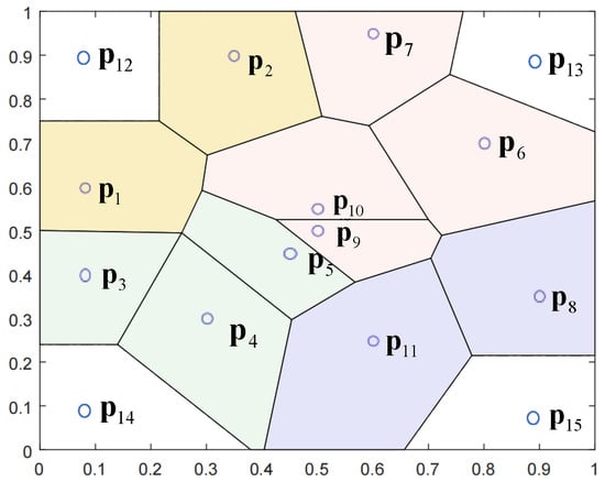
Figure 1.
Voronoi diagram.
Voronoi neighbors are defined as seed points that share a Voronoi boundary. When Voronoi diagrams are applied in the field of multi-robot systems, each seed point is typically considered the position of a certain robot.
The construction of Voronoi diagrams is a challenging problem, primarily facing difficulties such as high computational complexity and challenges in high-dimensional space. The most commonly used construction methods include the Delaunay triangulation method and hyperplane construction method. In the sequel, these two constructing methods are introduced in detail.
2.1. Method 1: Delaunay Triangulation Method
In practice, how to construct the boundaries and vertices of the Voronoi regions has much significance. Delaunay triangle is a special type of triangle where the circumcircle of any triangle does not contain any other points [28]. It is typically used to generate a Voronoi diagram because its edges serve as the perpendicular bisectors of the edges of the Voronoi diagram, the detailed schematic is shown in Figure 2. The circumcenter of the Delaunay triangle serves as the Voronoi diagram vertex. Algorithm 1 illustrates the construction progress.
| Algorithm 1 Constructing Voronoi diagram with Delaunay triangulation. |
|
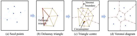
Figure 2.
Delaunay triangulation construction method.
In a multi-robot collaborative scenario, to construct the Voronoi cells, the robots considered as seed points only need to know the positions of adjacent robots, while not requiring the positions of other robots in the environment. Hence, the above strategy is indeed a distributed method [29].
2.2. Method 2: Hyperplane Construction Method
Calculating the hyperplanes between points is another method for constructing Voronoi diagrams [30], which is more suitable for constructing Voronoi regions in high-dimensional spaces compared to the Delaunay triangulation method, the schematic of this strategy is depicted as shown in Figure 3. In this method, the Voronoi boundary can be calculated as follows:
where and are hyperplane parameters used to calculate the Voronoi boundary, as shown in Figure 3b. Voronoi regions based on hyperplane construction can be represented as follows:
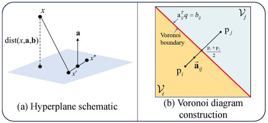
Figure 3.
Voronoi diagram construction method using hyperplanes.
In recent decades, with the advancement in technology, the Voronoi diagram theory has achieved fruitful research results. Figure 4 illustrates the technical development process of the Voronoi diagram. Among the existing results, four types of Voronoi diagrams are widely applied in the field of multi-robotics, namely the buffered Voronoi diagram [31], weighted generalized Voronoi diagram [32], uncertainty generalized Voronoi diagram [29], and discrete Voronoi diagram [33]. A detailed introduction to these types of Voronoi diagrams is given in the following:
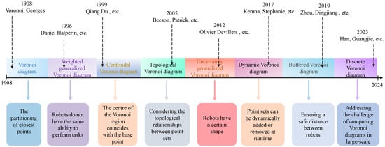
Figure 4.
Schematic diagram of the development of the Voronoi diagram.
- I.
- Buffered Voronoi diagram.
The buffered Voronoi diagram introduces the concept of a buffer zone to the traditional Voronoi diagram. It was first proposed to ensure a safe distance between robots to achieve collision avoidance.
Definition 1
(Buffered Voronoi diagram). The buffered Voronoi region of a robot can be defined as follows [31]:
where is the safety radius coefficient.
The buffered Voronoi diagram ensures collision avoidance by shrinking a safety radius around the perimeter of each robot’s Voronoi cell.
- II.
- Weighted generalized Voronoi diagram
In Equation (1), the basic Voronoi diagram divides the robot regions based solely on distance. However, in practical applications, robots may differ in their capabilities due to factors such as heterogeneity and energy capacity. Therefore, it is necessary to assign weights to robots when partitioning regions.
Definition 2
(Weighted generalized Voronoi diagram). Given the weight of robot i as and the weight of robot j as , the multiplication-weighted Voronoi region can be defined as follows [32]:
The boundaries of the partitioned regions are influenced by both weight and distance. The larger the weight is associated with robot i, the larger its Voronoi region. In real-world scenarios, the weight is determined based on different factors such as the ability of robots to perform tasks.
- III.
- Uncertainty generalized Voronoi diagram.
In real applications, due to the measurement noise or other unknown disturbances, it is difficult to obtain the accuracy position information; therefore, we cannot calculate the accuracy Voronoi region for each robot. To deal with this problem, the uncertainty-generating Voronoi diagram is proposed.
Definition 3
(Uncertainty generalized Voronoi diagram). Given two robots i and j, each with its own shape or uncertain region, and , the set of points that are closer to region than to region can be defined as follows [29]:
For robot i, considering the shape or uncertain region of the robot, the generalized Voronoi diagram can be defined as follows:
The boundary of the generalized Voronoi diagram of region relative to region is given by the following:
When obstacles exist in the environment or robots have characteristic shapes or uncertain regions, the generalized Voronoi diagram with uncertainty is of great significance.
- IV.
- Discrete Voronoi diagram
In large-scale or three-dimensional environments, constructing the basic Voronoi diagram in Equation (1) may lead to computational challenges and difficulties. It is feasible to initially partition the environment using a specific graph model, such as a grid model, and then calculate representative positions, such as centroids, within each grid region. Subsequently, the Voronoi calculation can be performed on these centroid positions. The discrete form of the Voronoi diagram is depicted in Figure 5. Due to its discrete nature, this method is also considered a type of Voronoi clustering [33].
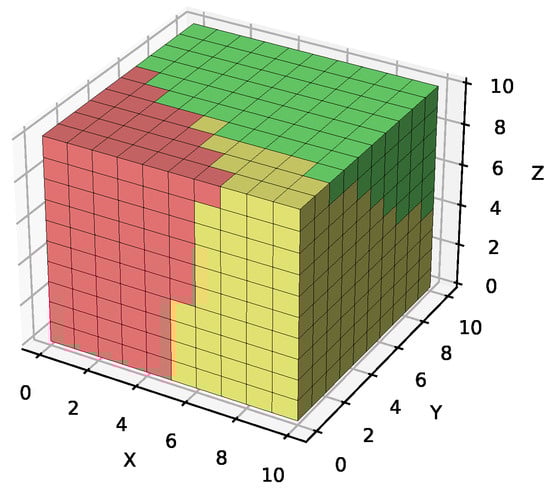
Figure 5.
Discrete Voronoi diagram.
Definition 4
(Discrete Voronoi diagram). The discrete form of the Voronoi diagram can be represented as follows [33]:
where represents the centroid positions of each subregion.
Other Voronoi diagrams in the field of multi-robotics include the following forms:
- Dynamic Voronoi diagrams facilitate the dynamic insertion or deletion of points during runtime, which is valuable in tasks such as robot path planning or base station optimization [34].
- Topological Voronoi diagrams consider the topological relationships between point sets based on distance relationships. They can be utilized to analyze network topology structures or road connections in map data [35].
- Centroidal generalized Voronoi diagrams are special types in which the centroid of each Voronoi region is as close as possible to the region’s base point, determined through iterative calculations. These diagrams have been widely applied in fields such as multi-robot coverage, numerical computation, computer graphics, and pattern recognition, among other fields [36].
Generally speaking, the primary roles of various forms of Voronoi diagrams in the environment can be summarized as region partitioning. However, they serve different purposes and functions across various practical application scenarios. In the following sections, this paper will comprehensively summarize the application methods and principles of Voronoi diagrams across two coverage task scenarios.
3. Coverage Methods Based on Voronoi Diagram
In this section, the problem of Voronoi diagram region coverage is categorized into two distinct types, based on sensor parameters: the task execution coverage problem and the sensor coverage problem. Moreover, a comprehensive overview of these two types of Voronoi diagram-based region coverage problems is presented.
3.1. Task Execution Coverage Problem
The Voronoi diagram-based task execution coverage scenario can be described as follows: given n robots in an environment Q, let and represent the two-dimensional position coordinates and control inputs of the i-th robot, respectively. According to [37], in task execution coverage, robots need to move to cover the entire environment, to meet the requirement of monitoring and rescue. In the multi-robot cooperative coverage issue under the Voronoi theory, each robot corresponds to a coverage area represented by its Voronoi region . It requires moving to suitable positions within the Voronoi regions to minimize the coverage cost. Figure 6 illustrates the entire process of the task execution coverage problem. In this scenario, the task execution coverage problem based on the Voronoi diagram can be described into the following two problems [38]:
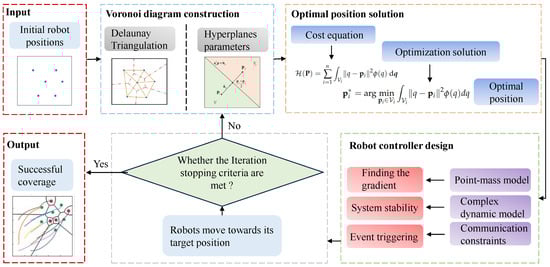
Figure 6.
Task execution coverage problem.
- Problem 1: Compute the optimal positions for the robots to minimize the coverage cost in the current scenario.
- Problem 2: Design an appropriate controller to ensure that the robot can move to the desired positions.
3.1.1. Optimal Position Solution
Under the Voronoi diagram framework, considering n robots that need to perform coverage tasks, the cost function for Problem 1 can be described as follows [38]:
where represents the Voronoi region of the i-th robot, q represents all points within the region. The cost function means the sum of distances between robot and all task locations q within . The smaller the value of , the fewer resources the covering robots need to cover all points q, indicating better coverage effectiveness.
When the robot position changes, the Voronoi diagram and the corresponding cost function also vary. To achieve the optimal coverage cost, it is necessary to move the robot to the optimal positions. Therefore, for the i-th robot, the optimization equation for Problem 1 can be defined as follows:
In a large-scale environment, different positions may have different levels of importance, making it unsuitable to define the cost function only by considering the distance between robots. Hence, the cost function for Problem 1 can be further described as [38]:
where represents a weighted function for position q, which is also referred to as a density function. It defines the importance of q in certain scenarios.
The coverage cost function not only considers the distance coverage function but also further takes into account the weights of task locations q, which is significant in practical applications. For instance, in maritime patrol scenarios, certain areas may be designated as high-priority surveillance zones, requiring more resources to complete patrol tasks in those areas. In such cases, it is necessary to set an appropriate weight function (density function) to describe the importance of q. Then, the optimization solution can be calculated as follows:
Solving optimization problems (13) is challenging. Typically, the optimal solution is obtained by taking the partial derivative of the optimization equation with respect to . The differentiation is as follows:
where represents the weighted area of the Voronoi region , and denotes the weighted centroid of the Voronoi region.
Equation (14) indicates that this method only calculates the optimal position within the Voronoi region of ; thus, it is a local optimization method rather than a global optimization method. This limitation poses a significant drawback to such methods. Recognizing this challenge, ref. [37] tackles this by formulating a dual function based on the cost function described in Equation (12)
where and satisfy the following conditions:
Subsequently, by analyzing the Lyapunov stability conditions of the controlled system, the optimal solution of the equation is derived. Compared to the traditional form of the cost function, this approach demonstrates greater capability in overcoming local optima and achieving superior control effectiveness.
Equation (14) implies that the Voronoi centroid is a local optimal position that minimizes the coverage cost function. That means the robot should always move toward the weighted centroid of its Voronoi region to ensure that the coverage cost in (12) is minimized.
Note that in different practical scenarios, the cost functions of coverage tasks may be different. How to construct the density function based on real applications is an important and challenging issue for the cost function. It has been mentioned in Equation (12) that the density function determines the importance of task locations. To achieve more precise coverage within the Voronoi diagram framework, accurately describing the density equation is crucial [39]. The density equation can generally be divided into functions related to position and time-varying functions. Ref. [36] explores a function defined as , where represents the position of point q. Based on this position-based density function, refs. [38,40] investigate the problem of controlling diffusive pollution sources within the framework of the Voronoi diagram coverage. This research treated the density function as the concentration equation of pollutants in real-world scenarios, proposing a time-varying density function through fractional order partial differential equations. Additionally, refs. [41,42] suggest that the density function is closely related to exploration boundaries. Ref. [41] describes the likelihood of missing individuals within a region as a time-varying density function, assuming that the density function reaches its maximum value at the environmental boundary and steadily decreases with increasing distance from the boundary.
Ref. [43] points out that when the density function varies over time, the optimal position is no longer the centroidal point position described in (14), which means the optimal positions are typically not unique, making it difficult to find the global minimum positions. Ref. [44] simplifies the time-varying density function and transforms (14) into a Lyapunov function. Then, by iteratively minimizing the error, the optimal positions are determined. This strategy has been successfully applied in dynamically changing coverage environments, such as search and rescue for trapped individuals, wildlife monitoring, environmental pollution monitoring, and resource exploration.
Moreover, to deal with the time-varying density functions, ref. [45] derives the optimal positions by expressing the density function as an equation related to the motion of covering robots. According to [39], the factors affecting the density function are influenced by external factors and are unrelated to the coverage robots, making them typically difficult to obtain. Therefore, when the density function is unknown, some researchers focus on selecting local minima for computing suboptimal positions. Ref. [46] applied a distributed interpolation method to iteratively estimate the density function. Similarly, ref. [47] utilized an online learning approach to acquire the basis functions of the density function, with demonstrable convergence properties, assuming the density function is within a set of known functions. Additionally, ref. [48] initially conducted exploration tasks, subsequently approximating the function through Gaussian networks. These studies demonstrate that the error between the learned function and the true function remains bounded.
Note that traditional Voronoi diagrams rely on the Euclidean distance between the robot position and other points, q, in the environment. This setting assumes that robot has the same coverage capability for all points q, but this is not realistic in the real world. Ref. [49] uses the Euclidean distance function to formulate generalized Voronoi diagrams, as follows:
where , , and are integers.
This approach addresses the challenge posed by varying capabilities of covering robots within the task area. In Euclidean distance space, computing these generalized Voronoi diagrams is straightforward, but in non-Euclidean distance space, their computations become intricately complex [10]. Inspired by the concept of constructing generalized Voronoi diagrams using non-Euclidean distances, ref. [50] extended the task coverage method to environments with obstacles. The authors rigorously demonstrated the convergence of the coverage control approach. However, this proof is limited to Riemannian manifold spaces, raising the question of whether this method applies to generalized mappings [10].
Except for the above aspects, communication between robots and workload balance is important [51,52,53]. The cost function proposed in [54] integrates coverage range and communication constraints, aiming to maximize coverage while ensuring compliance with communication constraints between robots. Additionally, ref. [55] advocated for robots to maintain specific formations while executing coverage tasks. In this context, “reasonable” implies that all robots share similar workloads. To achieve this objective, the cost function is rewritten as follows:
where represents the area of the Voronoi workspace for the i-th robot, and represents the average area of all Voronoi regions. The additional term accomplishes the tracking task by minimizing the variance of the area.
Moreover, in some coverage scenarios, due to limitations in coverage capabilities, robots may also have restricted coverage areas. In certain scenarios, it is crucial to consider area constraints for each region while minimizing the cost function, a concept known as the load balancing problem [32]. According to [32,44], by reforming the problem into a constrained optimization problem, it can be expressed as follows:
where represents the equal-weighted area of each coverage region.
This paper introduces the Jacobi iterative algorithm to determine the weight distribution of the additive generalized Voronoi, ensuring compliance with area constraints. Moreover, in [56,57], the issue of river boundary changes is considered a coverage region boundary change problem.
3.1.2. Coverage Control Method
After obtaining the optimal positions through optimization equations, robots can move based on Lloyd’s algorithm [39]. The basic steps of Lloyd’s algorithm can be outlined as shown in Algorithm 2.
| Algorithm 2 Lloyd’s Algorithm for Robot Movement |
|
During the process where robots move to their optimal positions within their respective Voronoi regions, if the robot’s kinematic model follows a point-mass model, the controller is typically formulated as follows [28]:
where is a positive constant, and represents the target optimal position.
This controller ensures that the robot moves toward the target position. However, the stability of this controller has not been analyzed. Furthermore, when considering the position error between the robot and the target, the controller can take a proportional-derivative form [55], which can be expressed as follows:
where , and and are the proportional and derivative coefficients, respectively.
Using the robot’s kinematic model as a point-mass scenario is not suitable for real applications; therefore, some scholars focus on designing controllers under complex robot kinematic models. The controller design problem can be divided into two main aspects: a controller design considering the robot’s kinematic model and a controller design under communication constraints.
- Controller design for robots with a complex dynamic model
In general, the principle of a controller design for robots with complex dynamic models is that the error between the robot’s position and the target position should converge. To address the problem of pollutant diffusion, ref. [38] designed a PI fractional-order controller for robots used in coverage tasks, equipped with fractional-order motion systems. Simulation experiments demonstrate that this approach converges faster and exhibits smaller positional errors compared to other methods. Ref. [58] considered quadcopter drones with complex dynamics, a controller was designed to ensure convergence to optimal positions while avoiding collisions between robots. This method maintains stability even in the presence of drone failures or the introduction of new drones.
In [59], an adaptive controller design method for coverage UAVs in a 3D environment is proposed, leveraging CBF to manage uncertainties in the robot’s input matrix, such as actuator failure. In contrast, ref. [60] introduced a feedforward action into the system to address the slow convergence issue encountered during the robot’s movement to the optimal position. Furthermore, ref. [61] utilized a reinforcement learning framework to craft controllers for multi-coverage robots. The reduction in coverage quantity, delineated in (14), serves as the reward function. It is established based on the Lyapunov function of the coverage robots. Maximizing this reward is attained when robots converge to optimal positions. This approach proposes a model-free framework using an online actor–critic architecture and incorporates a feedforward neural network to approximate the tracking control action. The results indicate that in highly uncertain and dynamic coverage scenarios, this model-free adaptive control is preferable.
- Controller design under communication constraints.
The Voronoi diagram is indeed a distributed construction method, implying that in the area coverage task, robots require the positional information of their neighboring robots to delineate their Voronoi task regions and compute the optimal position [62]. In practice, to reduce the communication burden, event-triggered mechanisms have been a hot topic in multi-robot cooperation. In [63], a control strategy based on an event-triggered mechanism is proposed under the Voronoi diagram framework, obviating the necessity for real-time communication among adjacent robots. Instead, it employs an adaptive estimation parameter to approximate the centroid at the last trigger event. In [64], each robot triggers a communication update when the error between its state at the last communication trigger and the centroid of its Voronoi region surpasses a predefined threshold. Furthermore, ref. [65] delineated communication event-triggered mechanisms into three inquiries: collect state samples, update control signals, and transmit signals. The efficacy of this method was validated on a Voronoi diagram coverage model. Additionally, ref. [62] introduced a fully asynchronous communication approach grounded in an event-triggered mechanism. Their event-triggered broadcast algorithm determines when robots transmit information to others in the system without necessitating responses from other robots. Moreover, in communication-constrained scenarios, devising distributed controllers for robot coverage scenarios by predicting robot positions based on past information proves to be an effective approach. In [22], a comprehensive state estimator was developed for robots, leveraging both currently available information and past data.
In summary, the task execution coverage method based on Voronoi diagrams furnishes a robust mathematical framework that meticulously characterizes and scrutinizes the computation of optimal positions and robot movement processes. However, this method confronts the challenge of being ensnared in local optima, potentially leading to inadequate coverage in certain regions. Hence, it is imperative to analyze and enhance the method based on particular practical scenarios.
3.2. Sensor Coverage Problem
The sensor coverage problem involves strategically placing sensors in a specified area. The goal is to ensure maximum coverage within the sensor’s range, thus achieving comprehensive monitoring and detection of targets within the area. As depicted in Figure 7, the commonly used sensor models include sector sensors, circular sensors, and camera sensors. The sensing capability of sector sensors relies on both the sector angle and sensing distance, while it is determined by their sensing radius for circular sensors. Meanwhile, the camera sensors’ sensing capability is influenced by factors such as ground distance, camera offset angle, and camera resolution. Additionally, the sensing capability of sensors can also be represented by probability distributions or diminishing functions [66].
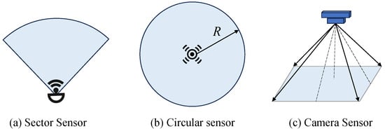
Figure 7.
Commonly used sensor models.
In practical applications, the goal of the sensor coverage problem is to achieve maximum coverage using minimal resources while avoiding coverage blind spots. Thus, the sensor coverage problem can be summarized into the following two objectives:
- Objective 1: How to deploy robot positions to minimize the overlap rate of sensor coverage.
- Objective 2: How to avoid coverage blind spots (coverage holes) during the deployment process of robot positions, as shown in Figure 8.
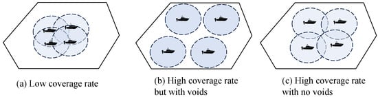 Figure 8. Coverage effectiveness diagram. In scenario (a), although the sensor coverage avoids holes, the overlap of larger sensor ranges leads to resource wastage. In contrast, scenario (c) maximizes the monitoring range while avoiding resource wastage by minimizing coverage holes.
To minimize the overlap rate of sensor coverage, it is necessary to design an appropriate movement strategy for sensor-carrying robots since the detection range of each sensor is fixed. As a distributed control method, the virtual force approach calculates the attractive and repulsive forces between nodes based on the positions of the robots and the sensor range. This ensures that the distance between robots exceeds a certain threshold, preventing overlap of sensor coverage. This method serves as an effective control strategy for sensor-carrying robots, expanding the deployment range of the sensors [67], as shown in Figure 9.
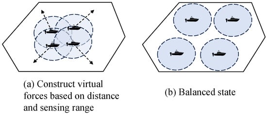
Figure 9.
Construct virtual forces based on the distance and sensing range.
However, virtual force algorithms operating alone cannot effectively address coverage holes in coverage scenarios. Some geometric features of computational geometry can be applied to analyze the geometric characteristics of sensor deployment, such as points, regions, and lines. The Voronoi diagram is a typical computational geometry method. Currently, combining the Voronoi diagram with virtual force methods to solve sensor deployment problems is an effective approach, which can maintain the coverage performance while avoiding coverage holes [68,69]. Refs. [69,70,71,72] defined the intersection of the sensor detection range and Voronoi regions as effective detection areas, as shown in Figure 10. Under this definition, ref. [69] proposed a Voronoi-based algorithm (VOR) to eliminate coverage holes. This algorithm recalculates virtual forces by computing the distance between robots and the vertices of Voronoi regions to reduce coverage gaps, as shown in Figure 10. Under the influence of these forces, robots equipped with sensors move to maximize the effective detection area while avoiding the coverage holes. Additionally, a minimax algorithm is also proposed in [69]. It is similar to the VOR but takes a more cautious approach, avoiding the emergence of new coverage gaps resulting from the excessive node relocation observed in the VOR method. However, this methodology solely addresses scenarios where all sensor detection ranges are uniform and cannot accommodate sensor heterogeneity.
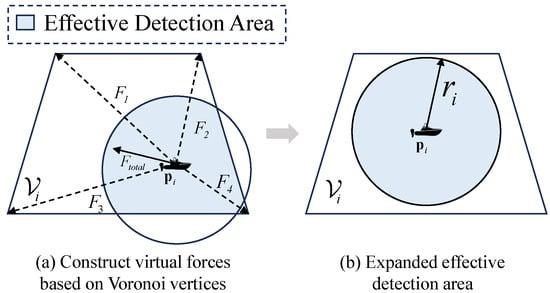
Figure 10.
Voronoi-based algorithm.
Note that the above results rarely consider the heterogeneous sensor scenario, in which the sensors’ detection ranges are different. For the heterogeneous sensor deployment problem, refs. [70,71,72] established an improved generalized weighted Voronoi based on the proportion of the sensor range. The authors considered the relative proportions of adjacent sensor ranges. Subsequently, the magnitude and direction of virtual forces for robot movement were computed based on the vertices and boundaries of the generalized weighted Voronoi diagram, indicating that it can effectively enhance coverage and mitigate coverage holes.
In summary, the virtual force-based sensor deployment method is intuitive and highly scalable in solving sensor coverage problems. However, it faces the risk of being trapped in local optima. Additionally, the stability of this method has not been thoroughly analyzed, which may not completely eliminate the occurrence of coverage gaps.
In other types of sensor coverage problems, ref. [73] investigated the coverage of UAVs carrying camera sensors. Essentially, this problem can be viewed as an optimization problem. Its optimization objective is to control the position information of the UAVs (altitude, location) to maximize the coverage range of the sensors. The coverage cost function related to camera sensors is defined as follows:
where represents the importance of location q in Q to be monitored. represents the conic Voronoi diagram [74]. represents the collection of USVs covering the environment Q. . . represents the perspective quality associated with the camera.
By calculating the gradient of , the USV controller that minimizes can be obtained as follows:
Although the controller in (22) can expand the detection range of the camera sensors, it cannot prevent coverage gaps. As the dual graph of the Voronoi diagram, Delaunay triangulation provides complementary information about the spatial distribution of points for the Voronoi diagram. It has the characteristic that no other points lie within the circumcircle of each triangle [75]. This property serves as the numerical basis for avoiding coverage holes. As shown in Figure 11, if sensor nodes are used as vertices to construct Delaunay triangles, and the circumradius d of a Delaunay triangle is greater than the sensing radius r of the sensors, the circumcenter of the triangle must lie outside the sensing range of any sensor. Therefore, a coverage hole exists [76].
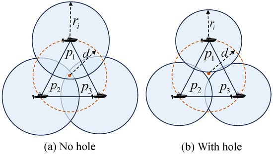
Figure 11.
Delaunay triangulation for detecting coverage holes.
The property of Delaunay triangles provides a numerical analysis foundation for computing robot motion strategies to avoid coverage holes. Ref. [77] used the Delaunay graph to develop a distributed gradient descent algorithm, which aims to reduce coverage gaps and increase the sensor coverage area. However, in a large-scale environment with multiple USVs, the aforementioned criteria are complex and demanding. Control barrier functions (CBFs) offer the forward invariance property to the admissible set of the robot state space, providing a robust framework for solving complex optimization problems [78,79]. CBFs have been successfully employed in various applications, ranging from bipedal robots [80,81] to swarm robots [82,83], and have also seen success in the context of environmental monitoring [84,85].
In [78], this CBF can be combined with Lyapunov functions in a quadratic programming framework. This approach helps achieve control objectives while maintaining acceptable system states, with the CBF acting as a constraint on the objective function. Inspired by the principles in [73,78], the authors constructed CBFs for coverage USVs, which can achieve hole-free coverage as shown in Figure 11. The optimization equation is formulated as follows:
Specifically, the CBF can be expressed as follows:
where are the positions of coverage robots. h is a continuously differentiable function. denotes the constraint of controller , which ensures that no coverage hole occurs.
In [66], the CBF is extended to a non-smooth version (NCBF) based on [73]. This extension enables quadcopters to operate in three-dimensional spaces and confirms that control inputs for quadcopters in this space exist, as long as the NCBF is satisfied.
In general, the method of constructing CBFs based on the characteristics of Delaunay triangles to prevent coverage holes exhibits good robustness. It is well-suited for larger environments or higher-dimensional spaces, showing strong scalability. However, the method may struggle to adapt to highly irregular or non-convex environments, where Delaunay triangulation might not accurately represent the space.
Concerning other camera sensors’ coverage methods under the framework of the Voronoi diagram, the cost function construction in [86] differs from the sensor model in Equation (21), as it considers the uncertainty of the sensor model during the coverage process. It is assumed that the UAV’s estimations of ground position and altitude entail distinct levels of uncertainty. As illustrated in Figure 12, the visual sensor’s perceptual range is denoted by the following:
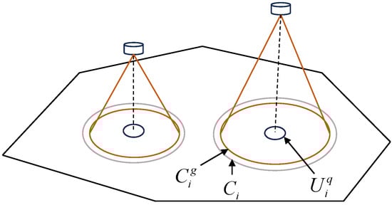
Figure 12.
Perception range of the camera considering localization uncertainty.
The region of uncertainty in the UAV’s position due to measurement errors from ground-based stations is represented by the following:
The conservative perceptual range considering these uncertainty regions is signified by the following:
Utilizing the uncertainties inherent in UAV localization and the variability in its perceptual range, researchers have employed an additive generalized Voronoi diagram to partition coverage areas for UAVs. Furthermore, similar to Equation (22), a control strategy for UAVs is designed in the presence of localization uncertainty, ensuring a continual expansion of coverage area while concurrently averting collisions among UAVs.
In sensor coverage problems, the evaluation metrics for coverage networks depend not only on maximizing coverage range but also on considering sensor energy consumption. In scenarios involving heterogeneous sensor coverage, sensors with larger detection ranges may deplete energy faster than other sensors, thereby reducing the monitoring performance of the sensor network. To address this issue, ref. [87] proposed a Voronoi–Laguerre technique; a specific Laguerre distance was defined for each sensor to determine the size of its responsible sensing region. To preserve energy, each sensor could adjust its sensing radius based on the size of its perceptual region. However, this method does not take into account the remaining energy of each sensor. To overcome this constraint, ref. [88] employed weighted Voronoi diagrams to construct sensing regions for heterogeneous sensors. In this approach, the sensing radius of sensors is adjustable. It aims to reduce overlapping detection areas while achieving energy savings. Additionally, sensors with the least remaining energy can further adjust their sensing radius with neighboring sensors, thereby maximizing the operational time of the sensor network.
Regarding the sensor energy consumption issue, ref. [89] also introduced a centralized immune-Voronoi deployment algorithm method, which relies on a binary probability model. It utilizes the characteristics of Voronoi diagrams to achieve a balance between coverage range and energy consumption. Similarly, ref. [90] proposed a coverage optimization technique that integrates firefly optimization, K-means algorithm, and Voronoi diagram techniques. This method optimizes the sensing radius to achieve maximum coverage with minimal sensor deployment. It combines multi-hop data transmission and circadian rhythm to reduce the energy consumption of deployed sensor nodes, thereby improving the network’s operational time. Ref. [91] developed an enhanced competitive swarm optimization algorithm to optimize sensor deployment, aiming to determine the optimal positions of sensor nodes to maximize coverage range. It then adjusts the sensing radius of each sensor based on the properties of the Voronoi diagram to achieve the best sensing radius configuration while minimizing energy consumption.
In conclusion, the sensor coverage method using Voronoi diagrams demonstrates strong generalization and scalability. It can adapt to various shapes and sizes of monitoring areas and integrates well with other methods, making it suitable for various coverage scenarios. Moreover, this method effectively reduces overlap and avoids coverage gaps, ensuring the effectiveness of coverage tasks. However, it has the drawback of increased computational complexity in large-scale sensor networks. Therefore, in practical applications, it is crucial to comprehensively assess the advantages and disadvantages of this method in specific environments and combine it with complementary methods for improvement.
4. Summary and Prospects
This paper presents a comprehensive overview of area coverage methods under the Voronoi diagram framework. The problem is categorized into task execution coverage and sensor coverage based on the involvement of sensor parameters, with detailed summaries and generalizations provided on model settings and solution methods tailored to practical scenarios. This paper aims to extract the key insights from existing literature and suggest potential avenues for future research.
Although the detailed summary above reveals significant progress in Voronoi-based region coverage methods, challenges still exist in some aspects. Therefore, this paper summarizes possible future directions in this field:
- Modeling coverage problems based on Voronoi diagram: Existing literature often collectively categorizes coverage problems as sensor coverage issues, lacking a unified and specific modeling framework. A model should comprehensively incorporate factors such as sensor perception models, communication conditions, obstacle models, and coverage cost/benefit functions.
- Communication failures and delays: In multi-robot cooperative coverage tasks, communication failures and communication delays are crucial factors that significantly impact the effectiveness of coverage tasks. However, to the best knowledge of the authors, in the framework of the Voronoi diagram, little attention has been paid to this issue. Therefore, designing effective coverage controllers for the MRS under communication failures or delays may be a future research direction.
- Robustness of coverage systems: Employing an MRS for environmental coverage offers distinct advantages over single robot coverage. However, in the MRS, devising effective robot coverage control strategies in the event of one or more robots failing presents another challenge for such methodologies.
- Local minimum problem in distributed methods: Voronoi diagrams are typically regarded as distributed methods. Each robot needs to utilize locally available information for coverage without access to global information. Most distributed algorithms confront the challenge of converging to local minimum solutions, which are suboptimal from a global perspective. Addressing the local optimum problem in Voronoi-based region coverage methods emerges as one of the future research directions.
- 3D region coverage: The issue of Voronoi region coverage in two-dimensional environments has received extensive attention. However, three-dimensional Voronoi region coverage poses considerably greater complexity compared to its two-dimensional counterpart. Existing two-dimensional coverage methods cannot be directly extrapolated to three-dimensional settings. Hence, the development of Voronoi-based region coverage methods suited for three-dimensional environments presents a challenging task for future research.
Author Contributions
Conceptualization, methodology, writing—review and editing, funding acquisition, M.Z.; investigation, methodology, writing-original draft preparation, J.L.; investigation, C.W.; supervision, project administration, J.W.; supervision, L.W. All authors have read and agreed to the published version of the manuscript.
Funding
This paper is funded by the National Key Research and Development Program of China (2023YFB4704404), the R&D Program of Beijing Municipal Education Commission (KM202410009014), and the Project of Cultivation for Young Top-notch Talents of Beijing’s Municipal Institutions (BPHR2022 03032).
Institutional Review Board Statement
Not applicable.
Informed Consent Statement
Not applicable.
Data Availability Statement
Data are contained within the article.
Conflicts of Interest
The authors declare no conflict of interest.
References
- Huang, M.H.; Rust, R.T. Engaged to a robot? The role of AI in service. J. Serv. Res. 2021, 24, 30–41. [Google Scholar] [CrossRef]
- Reis, J. Customer service through AI-Powered human-robot relationships: Where are we now? The case of Henn na cafe, Japan. Technol. Soc. 2024, 77, 102570. [Google Scholar] [CrossRef]
- Di, K.; Zhou, Y.; Jiang, J.; Yan, F.; Yang, S.; Jiang, Y. Risk-aware collection strategies for multi robot foraging in hazardous environments. ACM Trans. Auton. Adapt. Syst. 2022, 16, 1–38. [Google Scholar] [CrossRef]
- Mao, W.; Liu, Z.; Liu, H.; Yang, F.; Wang, M. Research progress on synergistic technologies of agricultural multi-robots. Appl. Sci. 2021, 11, 1448. [Google Scholar] [CrossRef]
- Paez, D.; Romero, J.P.; Noriega, B.; Cardona, G.A.; Calderon, J.M. Distributed particle swarm optimization for multi-robot system in search and rescue operations. IFAC-PapersOnLine 2021, 54, 1–6. [Google Scholar] [CrossRef]
- Pashna, M.; Yusof, R.; Ismail, Z.H.; Namerikawa, T.; Yazdani, S. Autonomous multi-robot tracking system for oil spills on sea surface based on hybrid fuzzy distribution and potential field approach. Ocean Eng. 2020, 207, 107238. [Google Scholar] [CrossRef]
- Zheng, H.; Li, Y.; Zheng, L.; Hashemi, E. Safe motion Planning and control framework for automated vehicles with zonotopic TRMPC. Engineering 2024, 33, 146–159. [Google Scholar] [CrossRef]
- Suo, Y.; Chen, X.; Yue, J.; Yang, S.; Claramunt, C. An Improved Artificial Potential Field Method for Ship Path Planning Based on Artificial Potential Field Mined Customary Navigation Routes. J. Mar. Sci. Eng. 2024, 12, 731. [Google Scholar] [CrossRef]
- Wu, Y.; Wang, T.; Liu, S. A Review of Path Planning Methods for Marine Autonomous Surface Vehicles. J. Mar. Sci. Eng. 2024, 12, 833. [Google Scholar] [CrossRef]
- Huang, S.; Teo, R.S.; Leong, W.W.; Martinel, N.; Forest, G.L.; Micheloni, C. Coverage control of multiple unmanned aerial vehicles: A short review. Unmanned Syst. 2018, 6, 131–144. [Google Scholar] [CrossRef]
- Cheng, C.; Sha, Q.; Li, G. Path planning and obstacle avoidance for AUV: A review. Ocean Eng. 2021, 235, 109355. [Google Scholar] [CrossRef]
- Yao, P.; Qiu, L.; Qi, J.; Yang, R. AUV path planning for coverage search of static target in ocean environment. Ocean Eng. 2021, 241, 110050. [Google Scholar] [CrossRef]
- Xu, P.F.; Ding, Y.X.; Luo, J.C. Complete coverage path planning of an unmanned surface vehicle based on a complete coverage neural network algorithm. J. Mar. Sci. Eng. 2021, 9, 1163. [Google Scholar] [CrossRef]
- Jung, Y.S.; Lee, K.W.; Lee, S.Y.; Choi, M.H.; Lee, B.H. An efficient underwater coverage method for multi-AUV with sea current disturbances. Int. J. Control Autom. Syst. 2009, 7, 615–629. [Google Scholar] [CrossRef]
- Tang, G.; Wang, C.; Zhang, Z.; Men, S. UAV Path Planning for Container Terminal Yard Inspection in a Port Environment. J. Mar. Sci. Eng. 2024, 12, 128. [Google Scholar] [CrossRef]
- Frasca, P.; Garin, F.; Gerencsér, B.; Hendrickx, J.M. Optimal one-dimensional coverage by unreliable sensors. SIAM J. Control Optim. 2015, 53, 3120–3140. [Google Scholar] [CrossRef]
- Song, C.; Feng, G. Coverage control for mobile sensor networks on a circle. Unmanned Syst. 2014, 2, 243–248. [Google Scholar] [CrossRef]
- Nivedhitha, V.; Baranidharan, B.; Santhi, B. A survey on coverage control protocols in wireless sensor networks. Int. J. Eng. Technol. 2013, 5, 635–641. [Google Scholar]
- Li, M.; Li, Z.; Vasilakos, A.V. A survey on topology control in wireless sensor networks: Taxonomy, comparative study, and open issues. Proc. IEEE 2013, 101, 2538–2557. [Google Scholar] [CrossRef]
- Mavrinac, A.; Chen, X. Modeling coverage in camera networks: A survey. Int. J. Comput. Vis. 2013, 101, 205–226. [Google Scholar] [CrossRef]
- Deif, D.S.; Gadallah, Y. Classification of wireless sensor networks deployment techniques. IEEE Commun. Surv. Tutorials 2013, 16, 834–855. [Google Scholar] [CrossRef]
- Miah, S.; Nguyen, B.; Bourque, A.; Spinello, D. Nonuniform coverage control with stochastic intermittent communication. IEEE Trans. Autom. Control 2014, 60, 1981–1986. [Google Scholar] [CrossRef]
- Chi, W.; Ding, Z.; Wang, J.; Chen, G.; Sun, L. A generalized Voronoi diagram-based efficient heuristic path planning method for RRTs in mobile robots. IEEE Trans. Ind. Electron. 2021, 69, 4926–4937. [Google Scholar] [CrossRef]
- Pan, T.; Yuan, Y. A region-based relay pursuit scheme for a pursuit–evasion game with a single evader and multiple pursuers. IEEE Trans. Syst. Man Cybern. Syst. 2022, 53, 1958–1969. [Google Scholar] [CrossRef]
- Zhu, J.; Yang, Y.; Cheng, Y. SMURF: A Fully Autonomous Water Surface Cleaning Robot with A Novel Coverage Path Planning Method. J. Mar. Sci. Eng. 2022, 10, 1620. [Google Scholar] [CrossRef]
- Pierson, A.; Wang, Z.; Schwager, M. Intercepting rogue robots: An algorithm for capturing multiple evaders with multiple pursuers. IEEE Robot. Autom. Lett. 2016, 2, 530–537. [Google Scholar] [CrossRef]
- Mo, Y.; Audrito, G.; Dasgupta, S.; Beal, J. Near-optimal knowledge-free resilient leader election. Automatica 2022, 146, 110583. [Google Scholar] [CrossRef]
- Xiao, F.; Yang, Q.; Bo, Z.; Hao, F. Distributed even coverage control of multi-robot systems. Control Theory Appl. 2023, 40, 441–449. [Google Scholar]
- Chevet, T.; Maniu, C.S.; Vlad, C.; Zhang, Y. Guaranteed Voronoi-based deployment for multi-agent systems under uncertain measurements. In Proceedings of the 2019 18th European Control Conference (ECC), Naples, Italy, 25–28 June 2019; pp. 4016–4021. [Google Scholar]
- Zhou, M.; Wang, Z.; Wang, J.; Cao, Z. Multi-robot collaborative hunting in cluttered environments with obstacle-avoided Voronoi cells. IEEE/CAA J. Autom. Sin. 2023. [Google Scholar] [CrossRef]
- Zhou, D.; Wang, Z.; Bandyopadhyay, S.; Schwager, M. Fast, on-line collision avoidance for dynamic vehicles using buffered Voronoi cells. IEEE Robot. Autom. Lett. 2017, 2, 1047–1054. [Google Scholar] [CrossRef]
- Cortés, J. Coverage optimization and spatial load balancing by robotic sensor networks. IEEE Trans. Autom. Control 2010, 55, 749–754. [Google Scholar] [CrossRef]
- Han, G.; Lai, W.; Wang, H.; Zhu, S. Hybrid algorithm-based full coverage search approach with multiple AUVs to unknown environments in internet of underwater things. IEEE Internet Things J. 2024, 11, 11058–11072. [Google Scholar] [CrossRef]
- Kemna, S.; Rogers, J.G.; Nieto-Granda, C.; Young, S.; Sukhatme, G.S. Multi-robot coordination through dynamic Voronoi partitioning for informative adaptive sampling in communication-constrained environments. In Proceedings of the 2017 IEEE International Conference on Robotics and Automation (ICRA), Singapore, 29 May–3 June 2017; pp. 2124–2130. [Google Scholar]
- Beeson, P.; Jong, N.K.; Kuipers, B. Towards autonomous topological place detection using the extended voronoi graph. In Proceedings of the 2005 IEEE International Conference on Robotics and Automation (ICRA), Barcelona, Spain, 18–22 April 2005; pp. 4373–4379. [Google Scholar]
- Du, Q.; Faber, V.; Gunzburger, M. Centroidal Voronoi tessellations: Applications and algorithms. SIAM Rev. 1999, 41, 637–676. [Google Scholar] [CrossRef]
- Inoue, D.; Ito, Y.; Yoshida, H. Optimal transport-based coverage control for swarm robot systems: Generalization of the voronoi tessellation-based method. IEEE Control Syst. Lett. 2020, 5, 1483–1488. [Google Scholar] [CrossRef]
- Chen, J.; Zhuang, B.; Chen, Y.; Cui, B. Diffusion control for a tempered anomalous diffusion system using fractional-order PI controllers. ISA Trans. 2018, 82, 94–106. [Google Scholar] [CrossRef] [PubMed]
- Lee, S.G.; Diaz-Mercado, Y.; Egerstedt, M. Multirobot control using time-varying density functions. IEEE Trans. Robot. 2015, 31, 489–493. [Google Scholar] [CrossRef]
- Chen, Y.; Wang, Z.; Liang, J. Optimal dynamic actuator location in distributed feedback control of a diffusion process. Int. J. Sens. Netw. 2007, 2, 169–178. [Google Scholar] [CrossRef]
- Haumann, D.; Willert, V.; Listmann, K.D. Discoverage: From coverage to distributed multi-robot exploration. IFAC Proc. Vol. 2013, 46, 328–335. [Google Scholar] [CrossRef]
- Macwan, A.; Nejat, G.; Benhabib, B. Target-motion prediction for robotic search and rescue in wilderness environments. IEEE Trans. Syst. Man, Cybern. Part B (Cybern.) 2011, 41, 1287–1298. [Google Scholar] [CrossRef]
- Liu, Y.; Wang, W.; Lévy, B.; Sun, F.; Yan, D.M.; Lu, L.; Yang, C. On centroidal Voronoi tessellation energy smoothness and fast computation. ACM Trans. Graph. (ToG) 2009, 28, 1–17. [Google Scholar] [CrossRef]
- Cortés, J.; Martinez, S.; Karatas, T.; Bullo, F. Coverage control for mobile sensing networks: Variations on a theme. In Proceedings of the Mediterranean Conference on Control and Automation, Lisbon, Portugal, 9–12 July 2002; pp. 9–13. [Google Scholar]
- Pimenta, L.C.; Schwager, M.; Lindsey, Q.; Kumar, V.; Rus, D.; Mesquita, R.C.; Pereira, G.A. Simultaneous coverage and tracking (SCAT) of moving targets with robot networks. In Algorithmic Foundation of Robotics VIII: Selected Contributions of the Eight International Workshop on the Algorithmic Foundations of Robotics; Springer: Berlin, Germany, 2010; pp. 85–99. [Google Scholar]
- Martinez, S. Distributed interpolation schemes for field estimation by mobile sensor networks. IEEE Trans. Control Syst. Technol. 2009, 18, 491–500. [Google Scholar] [CrossRef]
- Schwager, M.; Rus, D.; Slotine, J.J. Decentralized, adaptive coverage control for networked robots. Int. J. Robot. Res. 2009, 28, 357–375. [Google Scholar] [CrossRef]
- Schwager, M.; Vitus, M.P.; Powers, S.; Rus, D.; Tomlin, C.J. Robust adaptive coverage control for robotic sensor networks. IEEE Trans. Control Netw. Syst. 2015, 4, 462–476. [Google Scholar] [CrossRef]
- Guruprasad, K.; Ghose, D. Coverage optimization using generalized Voronoi partition. arXiv 2009, arXiv:0908.3565. [Google Scholar]
- Bhattacharya, S.; Ghrist, R.; Kumar, V. Multi-robot coverage and exploration on Riemannian manifolds with boundaries. Int. J. Robot. Res. 2014, 33, 113–137. [Google Scholar] [CrossRef]
- Dames, P.M. Distributed multi-target search and tracking using the PHD filter. Auton. Robot. 2020, 44, 673–689. [Google Scholar] [CrossRef]
- Lin, R.; Egerstedt, M. Dynamic multi-target tracking using heterogeneous coverage control. In Proceedings of the 2023 IEEE/RSJ International Conference on Intelligent Robots and Systems (IROS), Detroit, MI, USA, 1–5 October 2023; pp. 11103–11110. [Google Scholar]
- Luo, K.; Hu, B.; Guan, Z.H.; Zhang, D.X.; Cheng, X.M.; He, D.X. Distributed coordination of multi-agent systems for neutralizing unknown threats based on a mixed coverage-tracking metric. J. Frankl. Inst. 2020, 357, 12700–12723. [Google Scholar] [CrossRef]
- Kantaros, Y.; Zavlanos, M.M. Distributed communication-aware coverage control by mobile sensor networks. Automatica 2016, 63, 209–220. [Google Scholar] [CrossRef]
- Sun, W.; Dou, L.; Chen, J.; Fang, H. A multi-robot target tracking algorithm with centroidal Voronoi tessellation and consensus strategy. In Proceedings of the 29th Chinese Control Conference, Beijing, China, 29–31 July 2010; pp. 4607–4612. [Google Scholar]
- Abbasi, F.; Mesbahi, A.; Velni, J.M. A team-based approach for coverage control of moving sensor networks. Automatica 2017, 81, 342–349. [Google Scholar] [CrossRef]
- Abbasi, F.; Mesbahi, A.; Velni, J.M. A new Voronoi-based blanket coverage control method for moving sensor networks. IEEE Trans. Control Syst. Technol. 2017, 27, 409–417. [Google Scholar] [CrossRef]
- Elmokadem, T. Distributed coverage control of quadrotor multi-UAV systems for precision agriculture. IFAC-PapersOnLine 2019, 52, 251–256. [Google Scholar] [CrossRef]
- Bai, Y.; Wang, Y.; Xiong, X.; Song, J.; Svinin, M. Safe adaptive multi-agent coverage control. IEEE Control Syst. Lett. 2023, 7, 3217–3222. [Google Scholar] [CrossRef]
- Teruel, E.; Aragues, R.; López-Nicolás, G. A distributed robot swarm control for dynamic region coverage. Robot. Auton. Syst. 2019, 119, 51–63. [Google Scholar] [CrossRef]
- Soleymani, F.; Miah, M.S.; Spinello, D. Optimal non-autonomous area coverage control with adaptive reinforcement learning. Eng. Appl. Artif. Intell. 2023, 122, 106068. [Google Scholar] [CrossRef]
- Ajina, M.; Tabatabai, D.; Nowzari, C. Asynchronous distributed event-triggered coordination for multiagent coverage control. IEEE Trans. Cybern. 2020, 51, 5941–5953. [Google Scholar] [CrossRef] [PubMed]
- Zheng, Z.; Zhang, X.; Jiao, L. Optimized deployment of sensor networks based on event-triggered mechanism. In Proceedings of the 2018 37th Chinese Control Conference (CCC), Wuhan, China, 25–27 July 2018; pp. 7304–7309. [Google Scholar]
- Hayashi, N.; Muranishi, Y.; Takai, S. Distributed event-triggered control for voronoi coverage. In Proceedings of the 2015 International Conference on Event-Based Control, Communication, and Signal Processing (EBCCSP), Krakow, Poland, 17–19 June 2015; pp. 1–4. [Google Scholar]
- Nowzari, C.; Cortés, J. Self-triggered and team-triggered control of networked cyber-physical systems. In Event-Based Control Signal Process; CRC Press: Boca Raton, FL, USA, 2015. [Google Scholar]
- Funada, R.; Santos, M.; Maniwa, R.; Yamauchi, J.; Fujita, M.; Sampei, M.; Egerstedt, M. Distributed coverage hole prevention for visual environmental monitoring with quadcopters via nonsmooth control barrier functions. IEEE Trans. Robot. 2023, 40, 1546–1565. [Google Scholar] [CrossRef]
- Zou, Y.; Chakrabarty, K. Sensor deployment and target localization based on virtual forces. In Proceedings of the 2003 22th Annual Joint Conference of the IEEE Computer and Communications Societies, San Francisco, CA, USA, 30 March–3 April 2003; Volume 2, pp. 1293–1303. [Google Scholar]
- Qi, C.; Dai, H.; Zhao, X. Distributed coverage algorithm based on virtual force and Voronoi. Comput. Eng. Des. 2018, 39, 606–611. [Google Scholar]
- Wang, G.; Cao, G.; La Porta, T.F. Movement-assisted sensor deployment. IEEE Trans. Mob. Comput. 2006, 5, 640–652. [Google Scholar] [CrossRef]
- Mahboubi, H.; Moezzi, K.; Aghdam, A.G.; Sayrafian-Pour, K. Distributed deployment algorithms for efficient coverage in a network of mobile sensors with nonidentical sensing capabilities. IEEE Trans. Veh. Technol. 2014, 63, 3998–4016. [Google Scholar] [CrossRef]
- Mahboubi, H.; Aghdam, A.G. Distributed deployment algorithms for coverage improvement in a network of wireless mobile sensors: Relocation by virtual force. IEEE Trans. Control Netw. Syst. 2016, 4, 736–748. [Google Scholar] [CrossRef]
- Mahboubi, H.; Moezzi, K.; Aghdam, A.G.; Sayrafian-Pour, K. Distributed sensor coordination algorithms for efficient coverage in a network of heterogeneous mobile sensors. IEEE Trans. Autom. Control 2017, 62, 5954–5961. [Google Scholar] [CrossRef]
- Funada, R.; Santos, M.; Yamauchi, J.; Hatanaka, T.; Fujita, M.; Egerstedt, M. Visual coverage control for teams of quadcopters via control barrier functions. In Proceedings of the 2019 International Conference on Robotics and Automation (ICRA), Montreal, QC, Canada, 20–24 May 2019; pp. 3010–3016. [Google Scholar]
- Arslan, O.; Min, H.; Koditschek, D.E. Voronoi-based coverage control of pan/tilt/zoom camera networks. In Proceedings of the 2018 IEEE International Conference on Robotics and Automation (ICRA), Brisbane, QLD, Australia, 21–25 May 2018; pp. 5062–5069. [Google Scholar]
- Zhang, J.; Liu, J.; Ye, C. Area coverage algorithm based on region segmentation and Voronoi diagram. Appl. Res. Comput. 2020, 37, 3116–3120. [Google Scholar]
- So-In, C.; Nguyen, T.G.; Nguyen, N.G. An efficient coverage hole-healing algorithm for area-coverage improvements in mobile sensor networks. Peer-to-Peer Netw. Appl. 2019, 12, 541–552. [Google Scholar] [CrossRef]
- Kwok, A.; Martìnez, S. Unicycle coverage control via hybrid modeling. IEEE Trans. Autom. Control 2010, 55, 528–532. [Google Scholar] [CrossRef]
- Ames, A.D.; Xu, X.; Grizzle, J.W.; Tabuada, P. Control barrier function based quadratic programs for safety critical systems. IEEE Trans. Autom. Control 2016, 62, 3861–3876. [Google Scholar] [CrossRef]
- Ames, A.D.; Xu, X.; Grizzle, J.W.; Tabuada, P. Control barrier functions: Theory and applications. In Proceedings of the 2019 18th European Control Conference (ECC), Naples, Italy, 25–28 June 2019; pp. 3420–3431. [Google Scholar]
- Nguyen, Q.; Hereid, A.; Grizzle, J.W.; Ames, A.D.; Sreenath, K. 3D dynamic walking on stepping stones with control barrier functions. In Proceedings of the 2016 IEEE 55th Conference on Decision and Control (CDC), Las Vegas, NV, USA, 12–14 December 2016; pp. 827–834. [Google Scholar]
- Ahmadi, M.; Xiong, X.; Ames, A.D. Risk-averse control via CVaR barrier functions: Application to bipedal robot locomotion. IEEE Control Syst. Lett. 2021, 6, 878–883. [Google Scholar] [CrossRef]
- Wang, L.; Ames, A.D.; Egerstedt, M. Safety barrier certificates for collisions-free multirobot systems. IEEE Trans. Robot. 2017, 33, 661–674. [Google Scholar] [CrossRef]
- Funada, R.; Cai, X.; Notomista, G.; Atman, M.W.; Yamauchi, J.; Fujita, M.; Egerstedt, M. Coordination of robot teams over long distances: From Georgia tech to Tokyo tech and back-an 11,000-km multirobot experiment. IEEE Control Syst. Mag. 2020, 40, 53–79. [Google Scholar] [CrossRef]
- Notomista, G.; Egerstedt, M. Persistification of robotic tasks. IEEE Trans. Control Syst. Technol. 2020, 29, 756–767. [Google Scholar] [CrossRef]
- Santos, M.; Mayya, S.; Notomista, G.; Egerstedt, M. Decentralized minimum-energy coverage control for time-varying density functions. In Proceedings of the 2019 International Symposium on Multi-Robot and Multi-Agent Systems (MRS), New Brunswick, NJ, USA, 22–23 August 2019; pp. 155–161. [Google Scholar]
- Tzes, M.; Papatheodorou, S.; Tzes, A. Visual area coverage by heterogeneous aerial agents under imprecise localization. IEEE Control Syst. Lett. 2018, 2, 623–628. [Google Scholar] [CrossRef]
- Bartolini, N.; Calamoneri, T.; La Porta, T.; Petrioli, C.; Silvestri, S. Sensor activation and radius adaptation (SARA) in heterogeneous sensor networks. ACM Trans. Sens. Netw. 2012, 8, 1–34. [Google Scholar] [CrossRef]
- Chang, C.T.; Chang, C.Y.; Zhao, S.; Chen, J.C.; Wang, T.L. SRA: A sensing radius adaptation mechanism for maximizing network lifetime in WSNs. IEEE Trans. Veh. Technol. 2016, 65, 9817–9833. [Google Scholar] [CrossRef]
- Abo-Zahhad, M.; Sabor, N.; Sasaki, S.; Ahmed, S.M. A centralized immune-Voronoi deployment algorithm for coverage maximization and energy conservation in mobile wireless sensor networks. Inf. Fusion 2016, 30, 36–51. [Google Scholar] [CrossRef]
- Chowdhury, A.; De, D. Energy-efficient coverage optimization in wireless sensor networks based on Voronoi-Glowworm Swarm Optimization-K-means algorithm. Ad Hoc Netw. 2021, 122, 102660. [Google Scholar] [CrossRef]
- Musikawan, P.; Kongsorot, Y.; Muneesawang, P.; So-In, C. An enhanced obstacle-aware deployment scheme with an opposition-based competitive swarm optimizer for mobile WSNs. Expert Syst. Appl. 2022, 189, 116035. [Google Scholar] [CrossRef]
Disclaimer/Publisher’s Note: The statements, opinions and data contained in all publications are solely those of the individual author(s) and contributor(s) and not of MDPI and/or the editor(s). MDPI and/or the editor(s) disclaim responsibility for any injury to people or property resulting from any ideas, methods, instructions or products referred to in the content. |
© 2024 by the authors. Licensee MDPI, Basel, Switzerland. This article is an open access article distributed under the terms and conditions of the Creative Commons Attribution (CC BY) license (https://creativecommons.org/licenses/by/4.0/).