Abstract
Supercavitating vehicles present significant issues in controller design due to their multiphase flow-coupling characteristics. This study addresses force analysis and the construction of a 6-degree-of-freedom mathematical model for a supercavitating vehicle. A terminal sliding mode control law is intended to guarantee the quick tracking of the command signal for high-precision attitude control. To drastically lower the frequency of actuation and communication, a mechanism to trigger events is also introduced into the control link. A disturbance observer, which estimates system uncertainty using a non-recursive differentiator, improves the robustness of the system. The Lyapunov approach is used to prove that the system is stable. Numerical simulation results validate that the proposed method enhances control accuracy and robustness. The event-trigger mechanism reduces the execution frequency to 18.59%, effectively reducing the communication burden.
1. Introduction
Supercavitating vehicles have attracted extensive attention from researchers because of their good drag reduction characteristics. This is mainly due to the supercavitation phenomenon that occurs around the vehicle, leading to the formation of a void that envelops the supercavitating vehicle itself [1]. As a result, the resistance experienced by the supercavitating vehicle is greatly reduced, allowing it to maintain high-speed movement underwater. Unlike traditional underwater vehicles, supercavitating vehicles experience cavitation that almost entirely covers their bodies. Consequently, their movement underwater is primarily affected by thrust from the tail and by gravity forces and resistive forces acting on the parts of the vehicle that protrude outside the envelope—the head, the control surfaces, and parts of the rear of the vehicle. These sections experience planing force [2]. However, the presence of cavitation poses significant challenges to the design of the control system due to its strong nonlinearity and strong coupling characteristics [3].
In recent years, scholars have carried out a lot of research on the dynamic characteristics of and control methods for supercavitating vehicles. A maneuvering supercavity model is applied to model the planing forces acting on the vehicle in the vertical longitudinal plane [4,5,6,7], and a corresponding numerical algorithm is developed to simulate an uncontrolled vehicle making a diving motion in the longitudinal plane. L. Y. et al. [8] analyzed nonlinear physical phenomena for supercavitating vehicles under different cavitation numbers, and proposed a bifurcating control method to delay the Hopf bifurcation by adjusting the fin deflection angle, thus achieving stable movement. W. Z. et al. [9] used a maneuvering supercavity model with a cavitation number correction algorithm, proposing an exact linearizing feedback controller and a linear quadratic regulator for simulating the level flight, climbing, and diving of the vehicle. H. Y. et al. [10] established a linear parameter-varying (LPV) time-delay model for a supercavitating vehicle by analyzing the time-delay characteristics of the planing force, and designed a predictive controller based on the model.
Sliding mode control is widely used in the design of supercavitating vehicle control laws because of its robust performance and control accuracy. Z. X. et al. [11] designed a boundary sliding mode controller based on a disturbance observer in order to address the problem of strong nonlinearity in the longitudinal plane of a supercavitating vehicle. This controller allows for the accurate control of the depth and pitch angle by considering the estimated planing force boundary. It is specifically designed to handle time-delay characteristics and external disturbance conditions. In paper [12], a fractional sliding mode control law is designed to solve the complex maneuvering dynamics of the vehicle caused by factors such as undesired switching, delayed state dependency, and nonlinearities. W. J. et al. [13] developed a sliding mode controller based on a longitudinal model of a supercavitating vehicle. To compensate for system uncertainty, a radial basis function (RBF) neural network was used for observation and compensation. Y. Z. et al. [14] proposed a linear matrix inequality (LMI)-based cascade control to realize an efficient depth-tracking task, subject to actuator saturation. However, most of the current research on the dynamic characteristics and control of supercavitating vehicles is only carried out in terms of their longitudinal planes, and less attention is paid to controller design in yaw and roll channels.
In the process of high-speed navigation, due to inaccuracies in system parameter models, cavity oscillation, ocean current disturbances, and other interference effects, there is large deviation between the ideal system and the actual system in the controller design process, resulting in a reduction in control accuracy. In order to solve these uncertainties in the process of control system design, an adaptive law or an observer can be designed in order to observe the state and disturbance of the system, and feedback compensation can be applied in the control system to improve control accuracy and robustness. Y. H. et al. [15] addressed the motion control problem for an unmanned underwater vehicle in the presence of parametric uncertainties and time-varying external disturbances. A disturbance observer-based control scheme is proposed, which is structured around the integration of the model predictive control method with an extended active observer (EAOB). Compared to the conventional disturbance observer, the developed EAOB has the ability to handle both external disturbances and system/measurement noises simultaneously. In order to solve the influence of ocean currents and model uncertainties, V.M. et al. [16,17] designed a robust station-keeping (SK) control algorithm based on sliding mode control (SMC) theory for underwater vehicles, which ensured the control stability and better performance of a hovering over-actuated autonomous underwater vehicle (HAUV). To observe and compensate for unknown and complex environmental disturbances such as wind, waves, and currents, D. X. et al. [18] designed a nonlinear extended state observer (NESO). They then proposed a method that used a biologically inspired neural network (BINN) to reduce the input values of the initial state and solve the problem of thruster input saturation. In [19], nonlinear disturbance observer (NDO) was combined with the dynamic surface to design a moving wheel-inverted pendulum controller, which improved on the estimation of the disturbance. S. C. et al. [20] considered tracking control for a class of uncertain nonlinear systems, and proposed a nonsingular fast terminal sliding mode control scheme, combining RBF networks and disturbance observers. High-precision observation of the disturbance was achieved, enhancing the robustness of the system.
Finally, the control schemes currently proposed for supercavitating vehicles are all continuous control laws or time-triggered control laws. Due to the effect of external interference and its own uncertainty, the actuator used for control would not stay in the equilibrium position, but made continuous movements near it to ensure that the system’s states were maintained from the predetermined signals. The continuous operation of the actuator not only resulted in a serious waste of communication resources, but also causes more actuator wear and energy consumption. The introduction of an event-trigger mechanism (ETM) allows the controller-to-actuator signal to be updated in a way that is not dependent on the stimulus of time, but only on when preset trigger conditions are met. Therefore, this can effectively save the communication resources spent via transmission from the controller to the actuator, reduce the number and frequency of the actuator’s actions, and achieve the effect of saving energy and protecting the actuator [21]. In recent years, event-trigger mechanisms have been widely used in various control objects: H. G. et al. [22] proposed a distributed adaptive human-in-the-loop event-triggered formation controller for quadrotor unmanned aerial vehicles, with limited communication, system uncertainties, and unknown external disturbances in a highly uncertain and safety-critical environment. Aiming at the formation control of ground vehicle formations, a networked system with adaptive nonlinear coupling, a consistent control problem based on the observer, and event-trigger mechanisms were studied [23]. At the same time, the event-trigger mechanism was also studied in control problems for unmanned underwater vehicles and unmanned surface vessels [24,25,26].
Based on the above analysis of the limitations of supercavitating vehicle controller design, this paper makes innovative contributions in the following areas:
- In terms of research objects, most of the current research in the field of supercavitating vehicle control focuses on the longitudinal plane, while ignoring the influence of roll and sideslip channels. In this paper, the influence of the three channels is considered in the 6-DOF (degree-of-freedom) dynamic model and control design.
- In terms of control design, the linear sliding mode method is mostly used in related fields, and the terminal sliding mode method is designed in this paper, achieving improved control performance.
- Combined with the event-trigger mechanism, it fills the gap of the event-trigger mechanism in the field of supercavitating vehicle control. Unlike other event-trigger mechanisms, the event-trigger mechanism designed in this paper acts in the control link without considering the change of state.
- For the treatment of system uncertainties, most of the uncertainties in the field of supercavitating vehicle control are estimated via adaptive law or an RBF neural network observer, and the non-recursive extended state observer is used in this paper to improve the observation accuracy and comprehensively improve the robustness of the control system.
The organization of this paper is as follows. In Section 2, an attitude dynamics model for a supercavitating vehicle is established to lay the foundation for the subsequent controller design. In Section 3, the design of a non-recursive observer is completed, followed by the design of a terminal sliding mode surface and reaching law. After that, the design of an event-trigger mechanism is completed, and system stability analysis is carried out based on the Lyapunov method. In Section 4, simulations are conducted of supercavitating vehicle attitude control under perturbation. Lastly, conclusions are presented in Section 5.
2. Supercavitating Vehicle 6-DOF Math Model
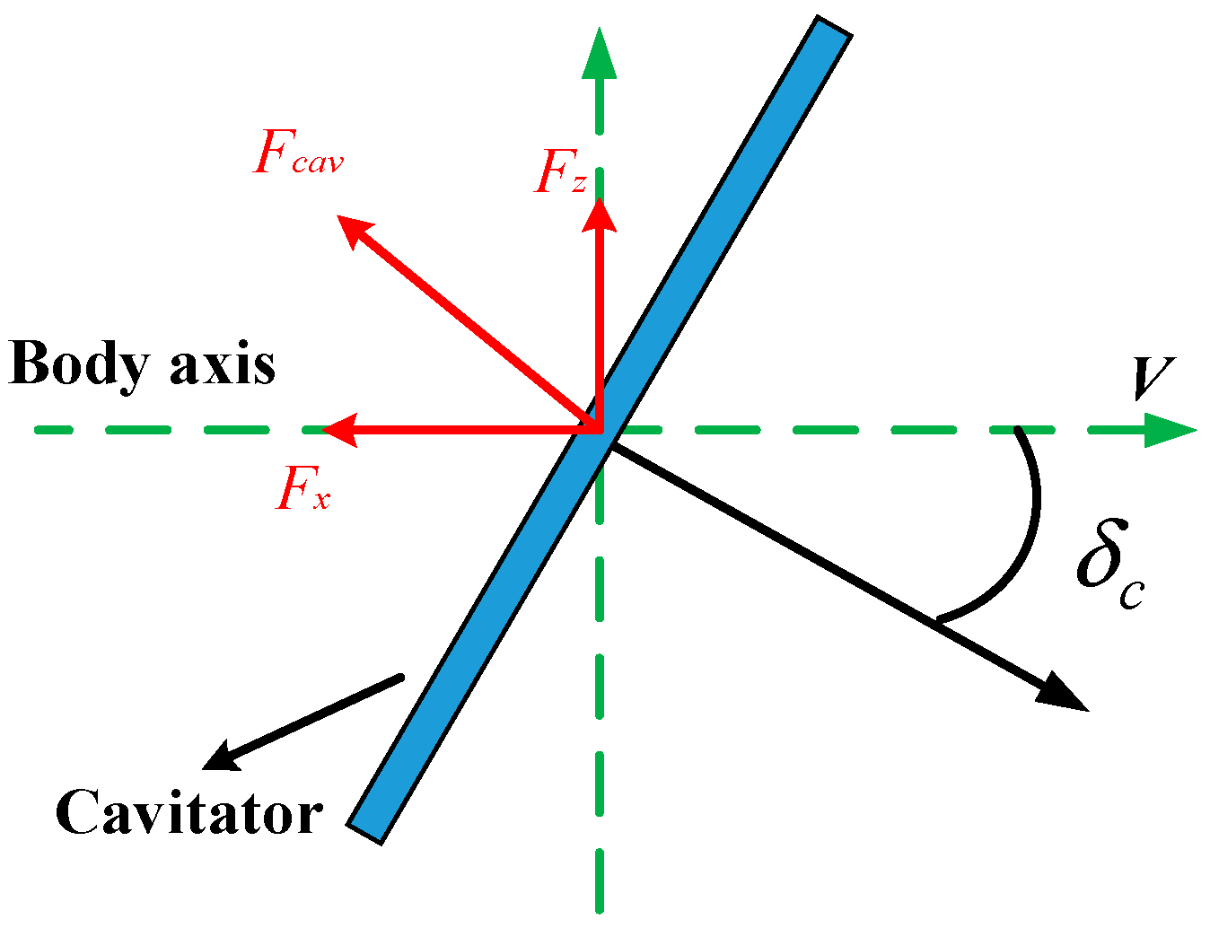
As shown in Figure 1, our proposed supercavitating vehicle model has two coordinate systems: an earth-fixed coordinate system and a body-fixed coordinate system . Before force analysis, the configuration of the supercavitating vehicle needs to be explained. The head of the supercavitating vehicle is a disc cavitator that induces cavity generation while also being able to rotate in the vertical longitudinal plane in order to provide a pitch control effect. The body part is a long and slender cone and cylinder, which allows for most of it to be wrapped by a supercavity, thereby achieving load reduction and drag reduction. Assessed based on the above configuration, the forces acting on the supercavitating vehicle are also shown in Figure 1. The control actuators comprise the head cavitator and the fins at the tail.

Figure 1.
Definition of coordinate systems and force analysis of supercavitating vehicle.
The forces acting on the supercavitating vehicle can be described as gravity, planing force, thrust, and the forces acting on the cavitator and fins, resulting in the following equations of motion:
where is gravity acceleration, is the force acting on the cavitator, is the force acting on the fins, denotes the planing force, and represents the thrust of the main engine for the supercavitating vehicle. is the transformation matrix from body to inertial coordinate , which can be presented as follows:
Remark 1.
In the model established in this paper, the drag of the fins and the resistance of the planing force are neglected, since they are negligible in comparison to force acting on the cavitator and the force acting on the fins in the vertical component.
The attitude dynamics model for the supercavitating vehicle is as follows:
where represent the pitch angle, yaw angle, and roll angle, and represent the angular velocities of the body coordinate system. Before analyzing the forces acting on a supercavitating vehicle, the following basic assumptions are given:
Assumption 1.
The supercavitating vehicle is an ideal rigid body, and the mass and centroid position remain constant, and do not change during the movement.
Assumption 2.
The supercavitating vehicle is a symmetrical rotary body, and the parameters of the pitch plane and the side slip plane are the same.
These forces and torques will be analyzed in detail in the following sections.
2.1. Supercavity Model
Firstly, we consider the morphology of the supercavity. The shape of the supercavity is related to the size of the head cavitator, the velocity of the vehicle, the static pressure of the surrounding water, and the vehicle depth. The definition of the cavitation number is given as follows:
where is the saturated vapor pressure of the water, and is the static pressure in still water. Overall, cavitation numbers characterize the relationship between pressure and dynamic pressure.
As Figure 2 shows, cavitation is induced by the cavitator at the head of the supercavitating vehicle, and the subsequent cavity cross-section is usually assumed to be a circle that develops along the central axis of the cavity. The radius of the cavity cross-section at a distance from the cavitator is defined as .

Figure 2.
The shape of the cavity.
Generally speaking, since most of the vehicle is surrounded by the cavity, it is not affected by hydrodynamics. Only the tail fins and the rear part of the body are affected by the cavity’s shape, and so only the cavity shape of the rear surface of the vehicle is calculated in this paper. On this basis, the cavity radius and rate of change at the tail of the vehicle are determined as follows:
where the virtual parameters are:
2.2. The Cavitator Force and Torque
The cavitator is an integral part of a supercavitating vehicle. It is required not only to induce the generation of supercavitation, but also to provide lift and pitch control for the supercavitating vehicle by rotating around its y-axis. The cavitator considered in this article only rotates in the vertical longitudinal plane, as Figure 3 shows.
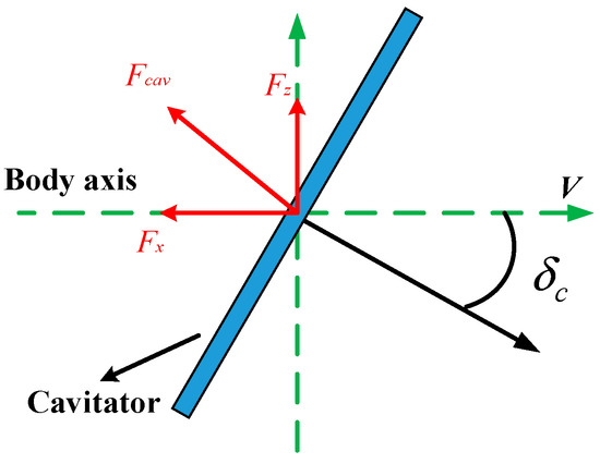
Figure 3.
Forces acting on the cavitator.
The force acting on the cavitator can be obtained in the body coordinate system, as follows:
where is the drag coefficient of the cavitator, is the fluid density, is the velocity of supercavitating vehicle centroid, is the cavitator area, is the cavitation number which characterizes the cavity’s morphological size, and is the control input.
The forces act on the center of the cavitator, and so the torques relative to the barycenter of the supercavitating vehicle are determined as follows:
where is the distance from the center of the cavitator to the barycenter of the supercavitating vehicle.
2.3. Gravity
Gravity acts on the center of mass of the supercavitating vehicle. This force can be obtained according to the coordinate conversion relationship:
Because the kinetic equation is based on the center of mass, it is not affected by the moment of gravity.
2.4. Fin Control Forces and Torques
In this paper, the cavitator and the elevators provide lift in order to maintain the depth of the supercavitating vehicle, while the rudders control the yaw and roll channels. As the Figure 4 shows, the hydrodynamic forces acting on the fins are closely related to the immersion ratios , which determine the control authority.
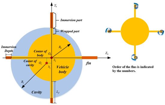
Figure 4.
The geometric relations between the vehicle body and the cavity at the tail.
The forces from the tail fins are additional to that of the cavitator. Considering the influence of wetting rate, the control forces from the four tail fins () on the vehicle body are as follows:
The control torques are as follows:
2.5. The Planing Force and Torque
Among the various fluid forces acting on supercavitating vehicles, the planing force is the most complex and the most nonlinear one. As Figure 5 shows, the planing force is the force acting on the part of the supercavitating vehicle that penetrates the cavity.
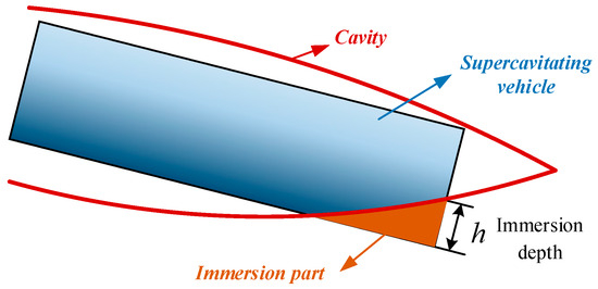
Figure 5.
The planning force of the supercavitating vehicle.
In planing force modeling methods, it is assumed that the planing force depends entirely on the vertical velocity. Logvinovich gave the following set of equations for the cylindrical body’s planing force and moment [27].
where is the distance between the tail and the center of the gravity, is the immersion angle, and the is the immersion depth.
The cavity shape at the tail is closely related to the cavitator angle of attack and the sideslip angle . The total cavitator angle of attack defines the direction of the planing force, and the angle defines the angle between the plane of immersion and the vertical symmetry axis of the cavity cross-section.
The planing forces in the body frame are obtained via projections of the plane of immersion into the x–y and x–z planes, and the resulting moment is perpendicular to this plane.
The parameter is expressed as follows:
The immersion angle is expressed as follows:
3. Event-Triggered Terminal Sliding Mode Control Based on Non-Recursive Observer
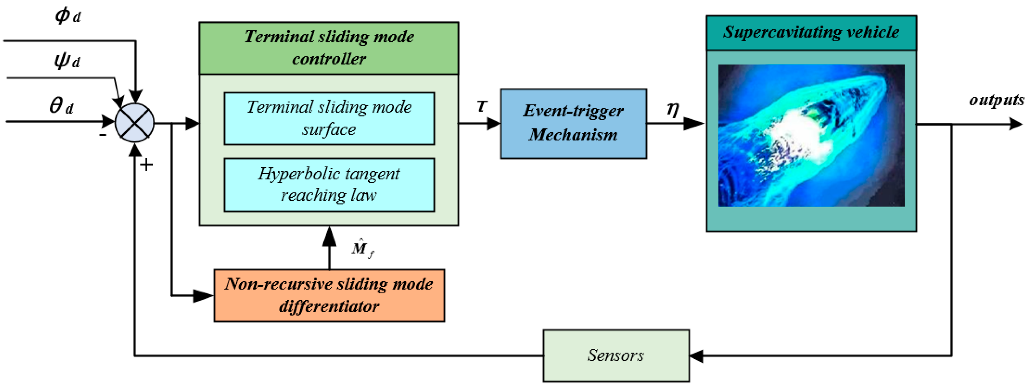
The design for the attitude control of a supercavitating vehicle utilizes a terminal sliding mode control algorithm. To enhance robustness, a non-recursive sliding mode differentiator with a model reference form is designed to observe the disturbance of the system. Moreover, an event-trigger mechanism for controlling quantity is developed to minimize the communication load. These design features collectively contribute to the robustness of the system. Figure 6 presents the framework of the control algorithm proposed in this study.

Figure 6.
Control structure of a supercavitating vehicle based on terminal sliding mode control and observer.
3.1. The Control Model
In this section, the control dynamics of the supercavitating vehicle are first deduced and rewritten into a form that facilitates the design of the controller. Defining as , and the control inputs as , the dynamics can be written as follows:
where , , .
Let be the desired signal. Then, define . Its time derivatives can be derived as follows:
where .
In the process of high-speed maneuvering, uncertainty regarding system modeling exists due to cavitation perturbation, system modeling parameter errors, and external interference . Considering the external disturbance caused by cavity perturbation, let . Thus, Equation (17) can be rewritten as follows:
Assumption 3.
Considering the actual situation, it is reasonable to assume that the external interference is bounded, that is, there is a value such that .
Remark 2.
The use of is only for the convenience of derivation, and the inverse solution calculation is required when calculating the specific declination angle of the actuators.
3.2. A State Observer Based on a Non-Recursive Differentiator
As mentioned in the previous section, there is a systemic uncertainty in the modeling of supercavitating vehicles. In this section, to enhance the robustness and control accuracy of the control system, a model reference state observer is designed by incorporating the modeled dynamics. The approach from [28] is utilized for the treatment of the state observer, and simultaneously, inspiration is drawn from the non-recursive differentiator employed in papers [29] and [30]. The observation output is introduced into the feedback link, and compensation is made in the control signal.
Consider the following generic dynamic system
where is the system state, is the output, is a smooth enough external disturbance, and and are known functions. The scalar output can be measured. is the output matrix.
An observer reconstructing the output and derivatives , for a finite time can use an n-th order non-recursive sliding mode differentiator, which takes the following form in the present case:
The function is defined as follows:
where the signum function is defined as follows
The exponents are selected as follows: satisfies the recurrent relations , , and , where belongs to an interval for a sufficiently small constant . The following Hurwitz matrix can be formed with the observer gains
After completing the above definition, the following lemma applies to the observer:
where is the estimation error, , , , , and . is a symmetric positive definite matrix; the symmetric positive matrix satisfies a Lyapunov equation:
where the matrix is defined above and is selected to be a positive definite matrix, is the minimum eigenvalue of the matrix , and is the maximum eigenvalue of the matrix .
Lemma 1 ([29,30]).
The observer state will converge to the vector of derivatives of the output
,
, within a finite time
Using the control model Equation (18), the above differentiator is used to reconstruct the error dynamics. Perturbation information is decomposed to realize the observation, so as to compensate in the control signal. An observer with a model reference is given as follows:
Design , , . We obtain
According to Lemma 1, the system will converge to zero in finite time, that is, when , the errors and converge to the origin.
3.3. Event-Triggered Terminal Sliding Mode Control Design
Before designing a controller, first give a lemma:
Then, the solution of the system is practical finite-time stable. The settling time satisfies , .
Lemma 2 ([28]).
Suppose that there exists a positive definite continuous Lyapunov function , with scalars
,
, and
such that
An event-trigger mechanism can effectively reduce the communication burden of the system and the actuator actuation frequency under the condition of sacrificing a small part of the control accuracy. In this paper, the following event-trigger mechanism is designed based on the control signal:
where and are the parameters of the event trigger, which are positive constants.
From Equation (29), we can deduce that
where are time varying parameters and satisfy . represents a unit vector.
Equation (30) can be organized into the following form
Based on the high-order derivative of the error signal, a non-singular terminal sliding mode controller is designed with a sliding surface:
where are control gain coefficient matrixes, which are positive and definite; are arbitrary constants and satisfy ; and the hyperbolic tangent function is smoother than the signum function and can better suppress chattering phenomenon.
When the sliding surface ,
Then, design a Lyapunov function,
Derivation yields
This shows that satisfies progressive stability, that is, when the sliding surface converges to zero, the error also converges to zero.
The control law is composed of two parts, an equivalent control law and a reaching control law :
where is the output of the observer, is a positive constant, is an event-trigger mechanism parameter, and and are control parameters of the reaching law.
Design a Lyapunov function
Differentiating with respect to time
Bringing Equation (31) into Equation (38) we have
Because , we then have
Expanding Equation (39) using Equations (40) and (36), we have
When the observer converges, there is a small value for which
Since is a small value, choose , and then .
Note that has the following property [31]:
where and .
In view of (43), Equation (42) can be derived as
Reuse Equation (40) and ,
Bringing Equation (45) into Equation (44) we have,
According to Lemma 2, it can be concluded that the system satisfies the stability conditions and can converge in finite time.
Next, it is proven that the Zeno behavior can be avoided in the event-trigger mechanism. Define the time interval as .
From (29), it follows that
Since is bounded, there is a positive constant satisfying . By noting that and when , there is . As such, it can be obtained that
Therefore, it can be obtained that the smallest interval is greater than zero. The Zeno behavior is successfully excluded.
Remark 3.
Zeno behavior refers to the fact that an event is triggered an infinite number of times in a finite amount of time. Therefore, when designing an event-trigger mechanism, you need to avoid two adjacent event-trigger intervals of less than or equal to zero. In a physical sense, there is no such thing as a time rewind or stop, but in a mathematical sense, there may be Zeno behavior. Therefore, when designing an event-trigger mechanism, it is necessary to prove that the system can avoid Zeno behavior.
4. Simulations
Combined with the control method proposed above, in this section, a simulation analysis is carried out with and without an event-trigger mechanism to discuss a reduction in the control communication frequency and the degree of control accuracy caused by the event trigger. Then, considering external disturbances, the convergence of the observer and the robustness of the controller are verified.
Firstly, the system parameters of the supercavitating vehicle (SV) in the simulation are given in Table 1.

Table 1.
Parameters of the simulated supercavitating vehicle.
Additionally, the control parameters are divided into a sliding surface, reaching law, and event-trigger mechanism; the parameters of the sliding mode surface are designed as , , , and ; and the reaching law parameters are , and . The parameters of the event-trigger mechanism are designed as , , and .
4.1. Simulation Analysis of the Effect of Event-Trigger Mechanism
Firstly, simulation analysis is carried out using the event-trigger mechanism. The effect of removing the event-trigger mechanism is simulated separately, and comparative analysis is carried out. In order to ensure rationality, the other control parameters are kept consistent in both cases. The desired control signal is , the initial value is and the specific simulation results shown below.
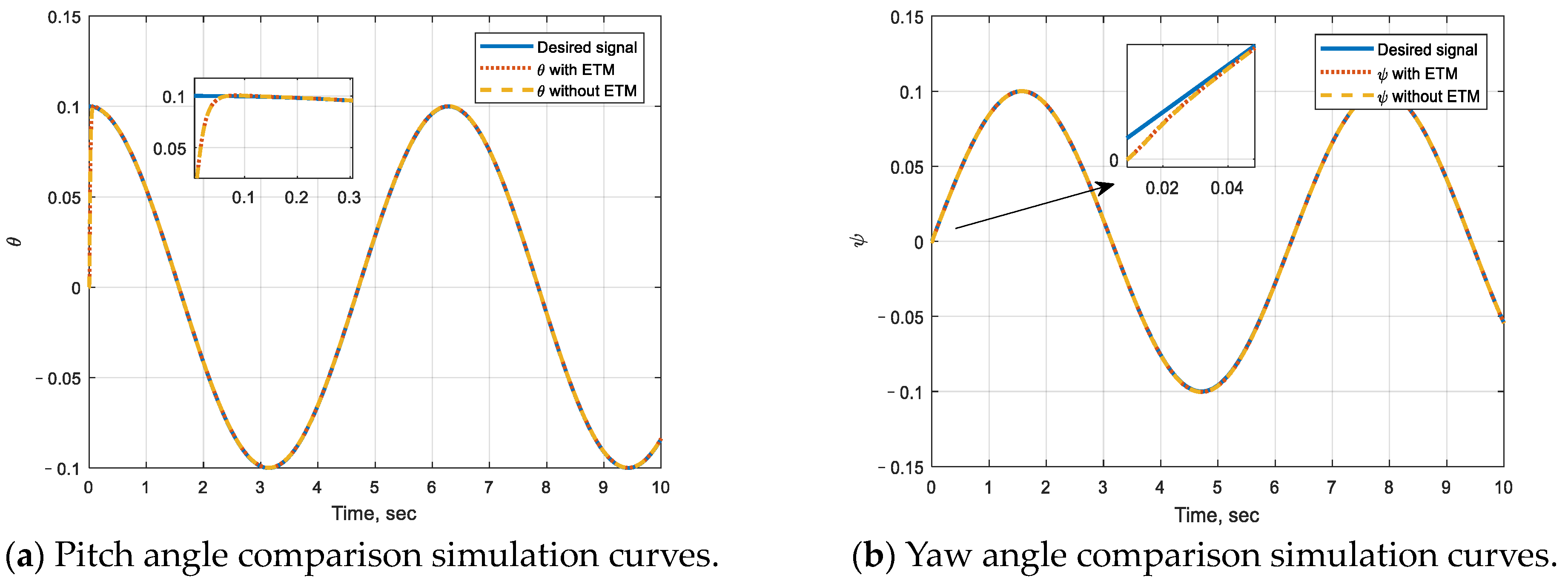
As the simulation results show in Figure 7 and Figure 8, it can be demonstrated that the control algorithm designed in this paper can track desired signals quickly and accurately, and the control accuracy and convergence speed is not greatly affected by the addition of the event-trigger mechanism.
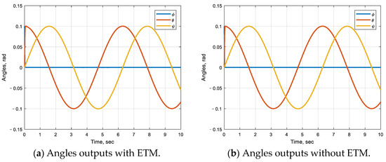
Figure 7.
Angles outputs’ comparison with/without ETM.
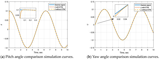
Figure 8.
Pitch angle and yaw angle comparison with/without ETM.
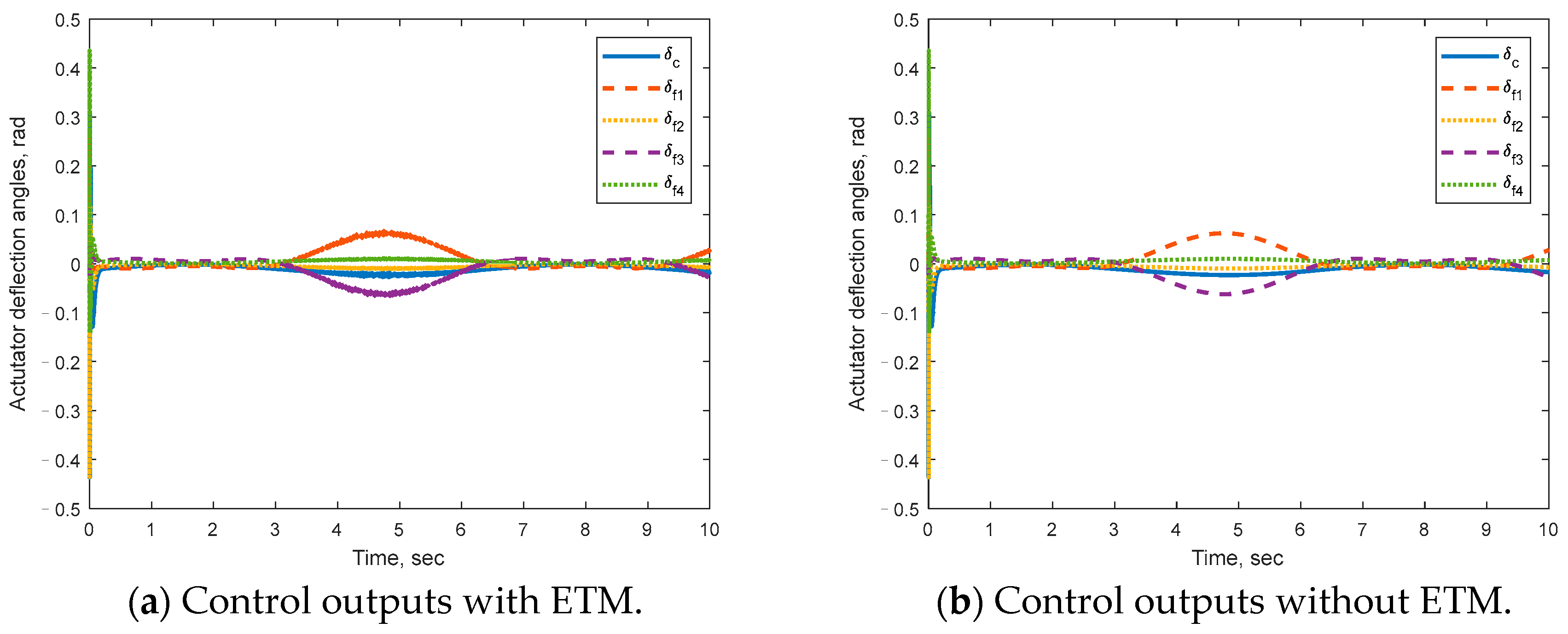
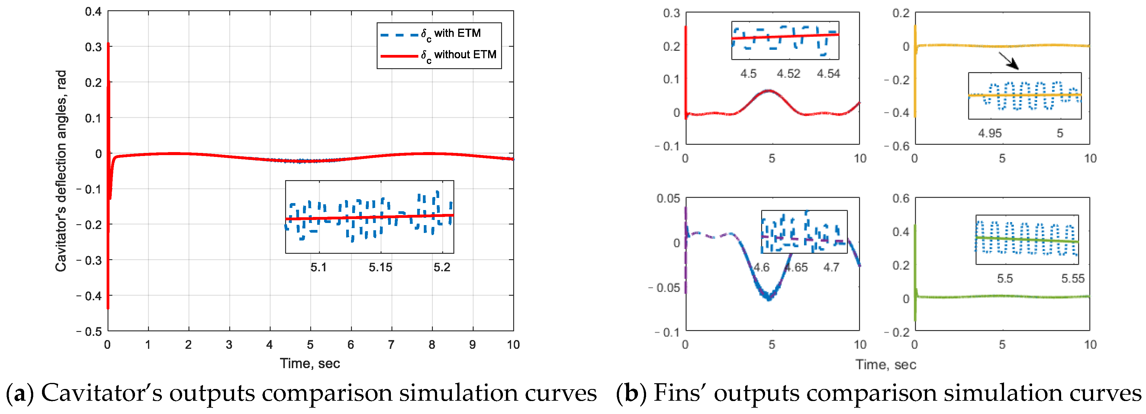
As the simulation results show in Figure 9 and Figure 10, after the event-trigger mechanism is added, the cavitator and fins’ operation is altered to follow a square wave pattern, indicating how the actuator changes as a result of the ETM.
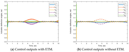
Figure 9.
Control outputs comparison with/without ETM.
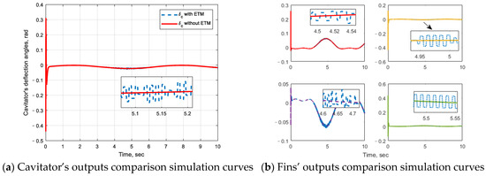
Figure 10.
Actuators’ deflection comparison simulation curves.
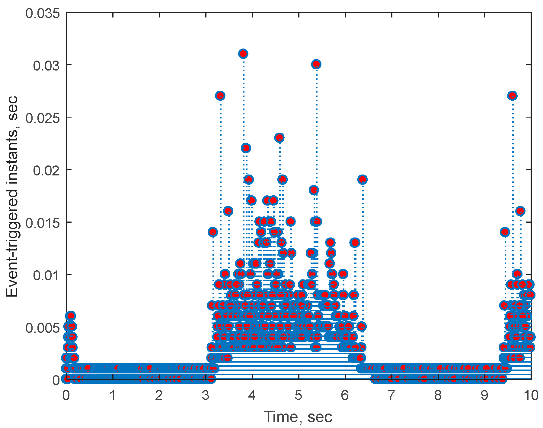
The proportion of time the actuator is instructed to move for is reduced to 17.39%, which greatly saves communication resources. The effectiveness of the event-trigger mechanism can be verified, and according to Figure 11, the red dot represents the moment when the event is triggered, while the value of its y-axis represents the time interval between two triggers, the Zeno phenomenon does not appear.

Figure 11.
Non-zero inter-event times.
4.2. Simulation Analysis in Perturbation
In order to verify the effectiveness of the state observer design, a simulation analysis is conducted under perturbation conditions, where the perturbation is given as , and the parameters of observer are designed as, , and .
In order to analyze the sensitivity of the proposed controller to the initial condition, the following two cases with different initial conditions are compared and simulated for analysis:
- Case 1: rad
- Case 2: rad
The specific simulation results are as follows:
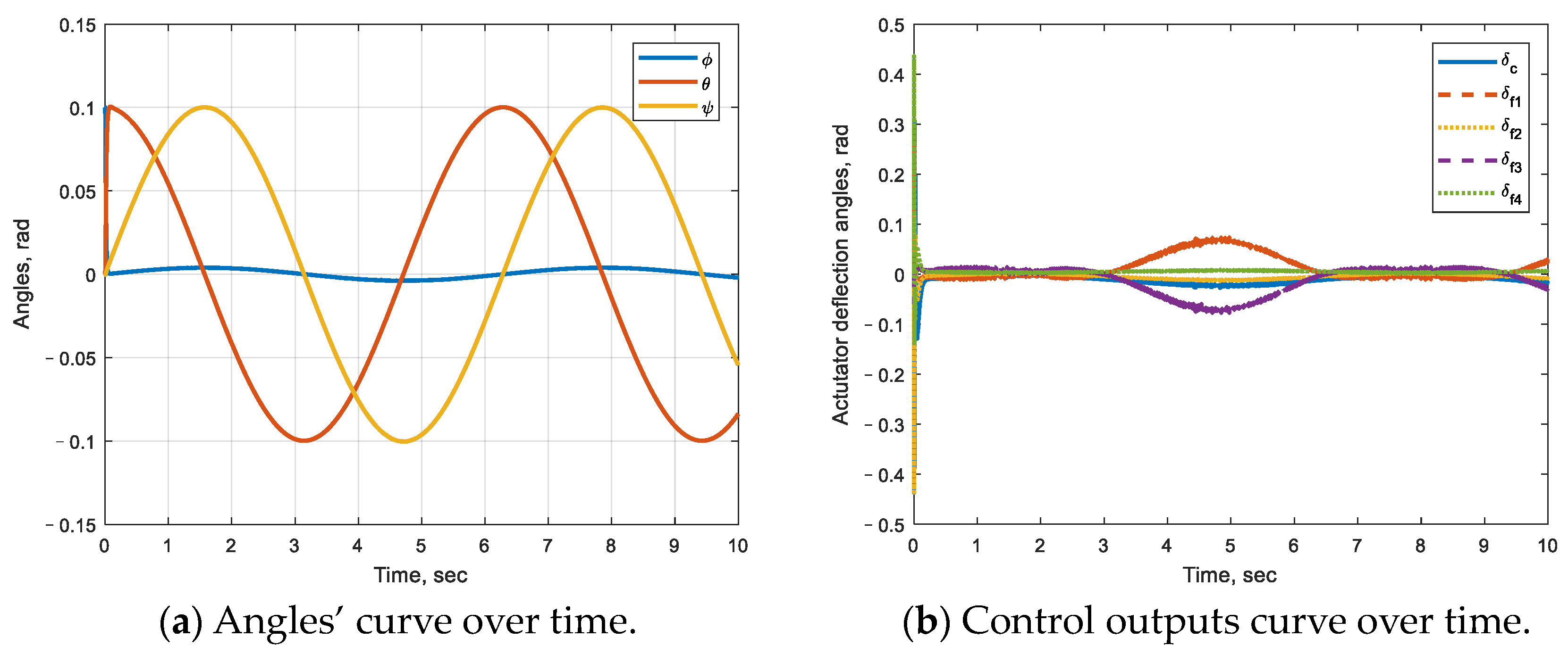
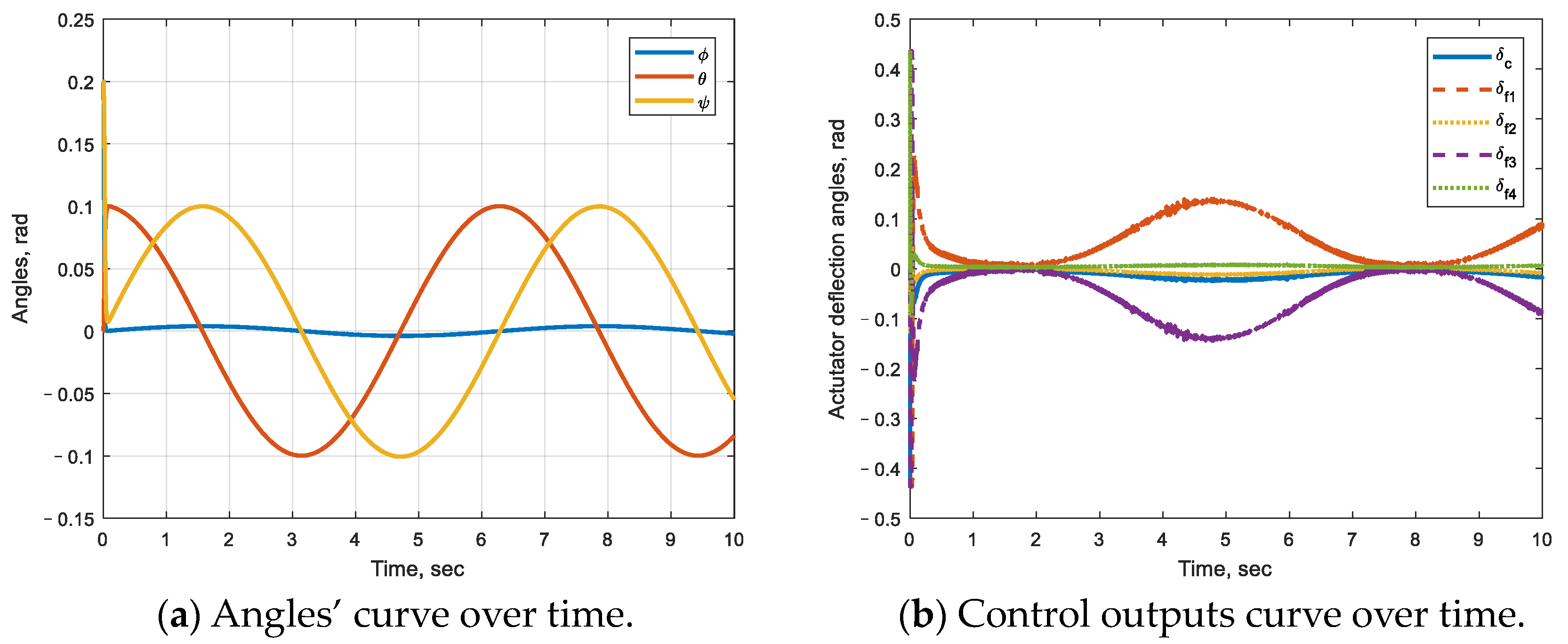
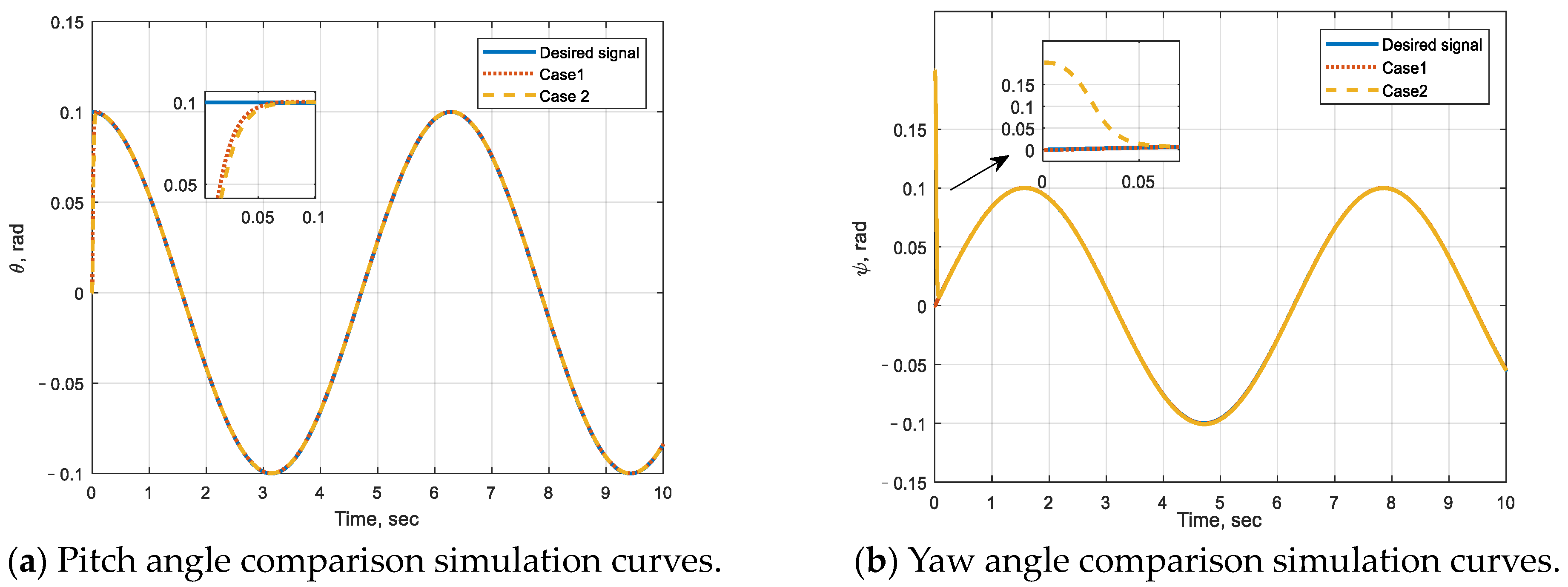
According to the simulation results Figure 12, Figure 13, Figure 14, Figure 15 and Figure 16, it can be seen that the control algorithm proposed in this paper can realize accurate control instructions, even if there is an external disturbance torque. According to the comparative simulation under two different initial conditions, it can be seen that the controller proposed in this paper has good adaptability to the initial conditions, and can achieve accurate tracking of the desired signal.

Figure 12.
Curves of state and control outputs with time under perturbation (Case 1).

Figure 13.
Curves of state and control outputs with time under perturbation (Case 2).
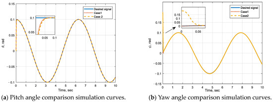
Figure 14.
Pitch angle and yaw angle comparison with 2 cases.
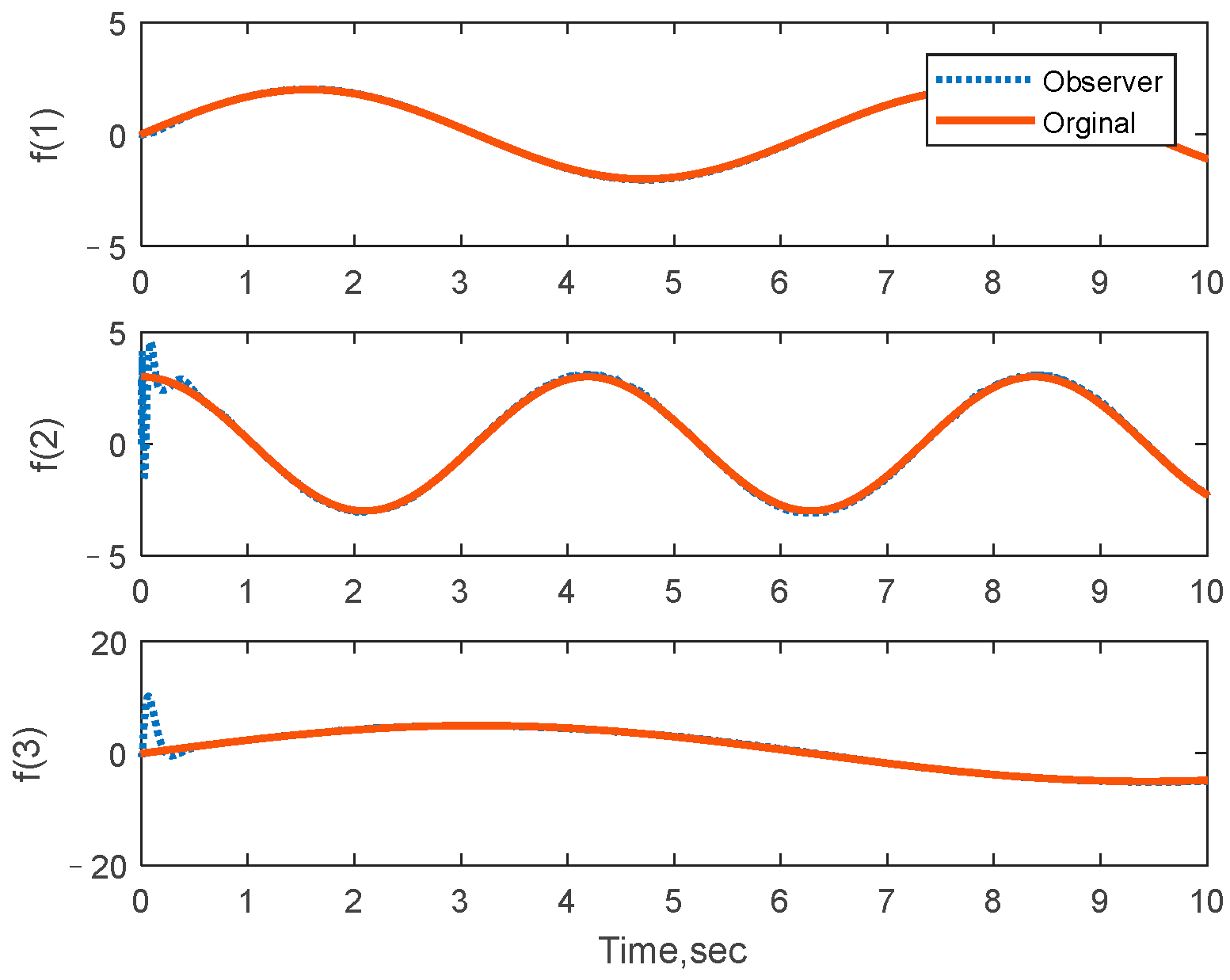
Figure 15.
The observer output compared to the given perturbation.
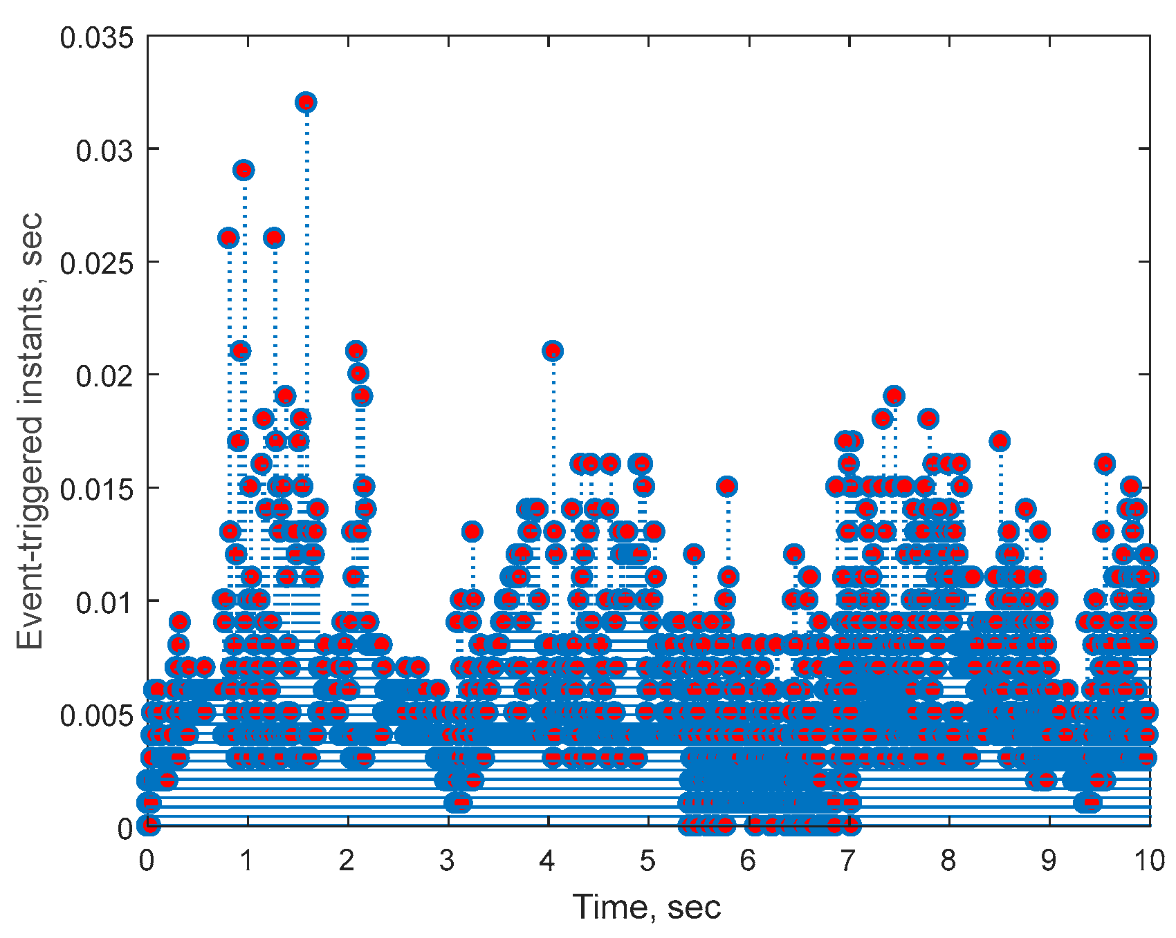
Figure 16.
The time and intervals of event trigger.
As the Figure 15 shows, the observer can accurately track the disturbance and compensate for it in the control system, which effectively improves the robustness and control accuracy of the control algorithm. According to the Figure 16, the event-trigger mechanism reduces the execution frequency to 18.59%, effectively reducing the communication burden.
5. Conclusions
In this paper, a 6-degree-of-freedom dynamic model was established for the supercavitating vehicle, considering the influence of roll and sideslip channels. In order to complete the attitude controller design, a control model of the supercavitating vehicle was derived, and the influence of uncertainties, such as cavitation perturbation, system modeling error, and external disturbance, was considered.
For the established attitude control model, we first designed a non-recursive extended state observer in the form of a model reference to realize the accurate observation of uncertainties. Combined with the event-trigger mechanism, the design of the terminal sliding mode controller is completed, and the Lyapunov stability criterion is used to prove that the error can converge to zero in finite time. It is also proved that the Zeno effect in the event-trigger mechanism can be avoided.
It is shown that the developed control approach can stabilize the error and converge it into a small neighborhood in finite time by applying a Lyapunov stability criterion. The simulation results demonstrate that the event-trigger-mechanism control strategy suggested in this research has a lower communication frequency and a better control effect, and that the designed observer can accurately observe the disturbances and compensate for them in the control system, which improves the robustness and control accuracy of the system.
At present, the controller designed in this paper has too many parameters that need to be adjusted, and the effect of actuator saturation has not been considered. These problems will be solved in subsequent research.
Author Contributions
Conceptualization, Z.Z. and X.W.; methodology, Z.Z.; software, Z.Z.; validation, Z.Z. and X.W.; formal analysis, Z.Z. and Z.W.; investigation, Z.Z.; resources, Z.Z.; data curation, Z.Z. and S.W.; writing—original draft preparation, Z.Z. and X.W.; writing—review and editing, Z.Z.; visualization, Z.Z.; supervision, S.W.; project administration, Z.W.; funding acquisition, X.W. All authors have read and agreed to the published version of the manuscript.
Funding
This research was funded by the National Natural Science Foundation of China (NSFC) under Grant U20B2005.
Institutional Review Board Statement
Not applicable.
Informed Consent Statement
Not applicable.
Data Availability Statement
The data that support the findings of this study are available from the corresponding authors upon reasonable request.
Acknowledgments
The authors gratefully acknowledge the helpful comments and suggestions of the reviewers.
Conflicts of Interest
The authors declare no conflicts of interest.
References
- Dzielski, J.; Kurdila, A. A Benchmark Control Problem for Supercavitating Vehicles and an Initial Investigation of Solutions. J Vib. Control 2003, 9, 791–804. [Google Scholar] [CrossRef]
- Zou, W.; Yu, K.; Arndt, R. Modeling and Simulations of Supercavitating Vehicle with Planing Force in the Longitudinal Plane. Appl. Math. Model. 2015, 39, 6008–6020. [Google Scholar] [CrossRef]
- Guo, H.; Han, Y.; Bai, T.; Zhou, Y.; Tai, X. Parameter-Dependent Robust Anti-Saturation Control of Supercavitating Vehicle with Time-Delay Characteristics. J. Vib. Control 2023, 29, 3340–3356. [Google Scholar] [CrossRef]
- Vanek, B.; Balas, G.J.; Arndt, R.E.A. Linear, Parameter-Varying Control of a Supercavitating Vehicle. Control Eng. Pract. 2010, 18, 1003–1012. [Google Scholar] [CrossRef]
- Lin, G.; Balachandran, B.; Abed, E.H. Dynamics and Control of Supercavitating Vehicles. J. Dyn. Syst. Meas. Control 2008, 130, 021003. [Google Scholar] [CrossRef]
- Mao, X.; Wang, Q. Nonlinear Control Design for a Supercavitating Vehicle. IEEE Trans. Contr. Syst. Technol. 2009, 17, 816–832. [Google Scholar]
- Mao, X.; Wang, Q. Adaptive Control Design for a Supercavitating Vehicle Model Based on Fin Force Parameter Estimation. J. Vib. Control 2015, 21, 1220–1233. [Google Scholar] [CrossRef]
- Lv, Y.; Wu, J.; Li, X.; Xiong, T. Influence of Fin Deflection Angle on Nonlinear Dynamic of Supercavitating Vehicle. IEEE Access 2021, 9, 134817–134825. [Google Scholar] [CrossRef]
- Zou, W.; Wang, B. Longitudinal Maneuvering Motions of the Supercavitating Vehicle. Eur. J. Mech. B/Fluids 2020, 81, 105–113. [Google Scholar] [CrossRef]
- Han, Y.; Xu, Z.; Guan, L. Predictive Control of a Supercavitating Vehicle Based on Time-Delay Characteristics. IEEE Access 2021, 9, 13499–13512. [Google Scholar] [CrossRef]
- Zhao, X.; Zhang, X.; Ye, X.; Liu, Y. Sliding Mode Controller Design for Supercavitating Vehicles. Ocean Eng. 2019, 184, 173–183. [Google Scholar] [CrossRef]
- Phuc, B.D.H.; Phung, V.-D.; You, S.-S.; Do, T.D. Fractional-Order Sliding Mode Control Synthesis of Supercavitating Underwater Vehicles. J. Vib. Control 2020, 26, 1909–1919. [Google Scholar] [CrossRef]
- Jinghua, W.; Yang, L.; Guohua, C.; Yongyong, Z.; Jiafeng, Z. Design of RBF Adaptive Sliding Mode Controller for A Supercavitating Vehicle. IEEE Access 2021, 9, 39873–39883. [Google Scholar] [CrossRef]
- Zhou, Y.; Li, J.; Sun, M.; Zhang, J.; Chen, Z. Cascade Control Design for Supercavitating Vehicles with Actuator Saturation and the Estimation of the Domain of Attraction. Ocean Eng. 2023, 282, 114996. [Google Scholar] [CrossRef]
- Hu, Y.; Li, B.; Jiang, B.; Han, J.; Wen, C.-Y. Disturbance Observer-Based Model Predictive Control for an Unmanned Underwater Vehicle. JMSE 2024, 12, 94. [Google Scholar] [CrossRef]
- Vu, M.T.; Le Thanh, H.N.N.; Huynh, T.-T.; Thang, Q.; Duc, T.; Hoang, Q.-D.; Le, T.-H. Station-Keeping Control of a Hovering over-Actuated Autonomous Underwater Vehicle under Ocean Current Effects and Model Uncertainties in Horizontal Plane. IEEE Access 2021, 9, 6855–6867. [Google Scholar] [CrossRef]
- Vu, M.T.; Le, T.-H.; Thanh, H.L.N.N.; Huynh, T.-T.; Van, M.; Hoang, Q.-D.; Do, T.D. Robust Position Control of an over-Actuated Underwater Vehicle under Model Uncertainties and Ocean Current Effects Using Dynamic Sliding Mode Surface and Optimal Allocation Control. Sensors 2021, 21, 747. [Google Scholar] [CrossRef] [PubMed]
- Xu, D.; Li, Z.; Xin, P.; Zhou, X. The Non-Singular Terminal Sliding Mode Control of Underactuated Unmanned Surface Vessels Using Biologically Inspired Neural Network. J. Mar. Sci. Eng. 2024, 12, 112. [Google Scholar] [CrossRef]
- Huang, J.; Ri, S.; Liu, L.; Wang, Y.; Kim, J.; Pak, G. Nonlinear Disturbance Observer-Based Dynamic Surface Control of Mobile Wheeled Inverted Pendulum. IEEE Trans. Contr. Syst. Technol. 2015, 23, 2400–2407. [Google Scholar] [CrossRef]
- Chen, S.; Liu, W.; Huang, H. Nonsingular Fast Terminal Sliding Mode Tracking Control for a Class of Uncertain Nonlinear Systems. J. Control Sci. Eng. 2019, 2019, 8146901. [Google Scholar] [CrossRef]
- Qian, Y.-Y.; Liu, L.; Feng, G. Output Consensus of Heterogeneous Linear Multi-Agent Systems with Adaptive Event-Triggered Control. IEEE Trans. Automat. Contr. 2019, 64, 2606–2613. [Google Scholar] [CrossRef]
- Guo, H.; Chen, M.; Jiang, Y.; Lungu, M. Distributed Adaptive Human-in-the-Loop Event-Triggered Formation Control for QUAVs with Quantized Communication. IEEE Trans. Ind. Inf. 2023, 19, 7572–7582. [Google Scholar] [CrossRef]
- Xu, Y.; Wu, Z.-G.; Pan, Y.-J. Observer-Based Dynamic Event-Triggered Adaptive Control of Distributed Networked Systems with Application to Ground Vehicles. IEEE Trans. Ind. Electron. 2023, 70, 4148–4157. [Google Scholar] [CrossRef]
- Li, X.; Pan, H.; Deng, Y.; Han, S.; Yu, H. Finite-Time Event-Triggered Sliding Mode Predictive Control of Unmanned Underwater Vehicles without Velocity Measurements. Ocean Eng. 2023, 276, 114210. [Google Scholar] [CrossRef]
- Zhang, G.; Han, J.; Zhang, W.; Yin, Y.; Zhang, L. Finite-Time Adaptive Event-Triggered Control for USV with COLREGS-Compliant Collision Avoidance Mechanism. Ocean Eng. 2023, 285, 115357. [Google Scholar] [CrossRef]
- Zhang, X.; Yao, S.; Xing, W.; Feng, Z. Fuzzy Event-Triggered Sliding Mode Depth Control of Unmanned Underwater Vehicles. Ocean Eng. 2022, 266, 112725. [Google Scholar] [CrossRef]
- Mirzaei, M.; Eghtesad, M.; Alishahi, M.M. Planing Force Identification in High-Speed Underwater Vehicles. J. Vib. Control 2016, 22, 4176–4191. [Google Scholar] [CrossRef]
- Fu, M.; Yu, L. Finite-Time Extended State Observer-Based Distributed Formation Control for Marine Surface Vehicles with Input Saturation and Disturbances. Ocean Eng. 2018, 159, 219–227. [Google Scholar] [CrossRef]
- Basin, M.; Yu, P.; Shtessel, Y. Finite- and Fixed-time Differentiators Utilising HOSM Techniques. IET Control Theory Appl. 2017, 11, 1144–1152. [Google Scholar] [CrossRef]
- Basin, M.V.; Yu, P.; Shtessel, Y.B. Hypersonic Missile Adaptive Sliding Mode Control Using Finite- and Fixed-Time Observers. IEEE Trans. Ind. Electron. 2018, 65, 930–941. [Google Scholar] [CrossRef]
- Ning, K.; Wu, B.; Wang, D. Velocity Observer-Based Event-Triggered Adaptive Fuzzy Attitude Takeover Control of Spacecraft with Quantized Quaternion. IEEE Trans. Aerosp. Electron. Syst. 2023, 59, 4168–4179. [Google Scholar] [CrossRef]


Disclaimer/Publisher’s Note: The statements, opinions and data contained in all publications are solely those of the individual author(s) and contributor(s) and not of MDPI and/or the editor(s). MDPI and/or the editor(s) disclaim responsibility for any injury to people or property resulting from any ideas, methods, instructions or products referred to in the content. |
© 2024 by the authors. Licensee MDPI, Basel, Switzerland. This article is an open access article distributed under the terms and conditions of the Creative Commons Attribution (CC BY) license (https://creativecommons.org/licenses/by/4.0/).