Numerical Investigation on a High-Speed Transom Stern Ship Advancing in Shallow Water

Abstract

A high-speed advancing ship will cause significant squats in shallow water, which could increase the risk of grounding. To this end, a program based on the Rankine higher-order boundary element method (HOBEM) is developed to investigate a high-speed displacement ship with a transom stern moving in shallow water. The nonlinear free surface condition is satisfied by adopting an iterative algorithm on the real free surface. The transom condition is considered by implementing a modified transom condition. Computations of wave-making resistance, sinkage and trim in deep water are first performed, and satisfactory agreement is achieved by comparing with the experimental results; the simulations are then extended to the shallow water case. It indicates that the present method can provide a suitable balance of practicability and robustness, which can be considered as an efficient tool for the guidance in ship design stage.

1. Introduction

Limited water depth has significant influences on the hydrodynamic performance of an advancing ship, especially for high-speed displacement vessels. The shallow water effects would accelerate the fluid flow between the ship and the bottom, which could lead to pronounced sinkage and trim, and thus cause the ship to ground. Moreover, the increased wash waves will not only induce large ship resistance, but also will damage other waterway infrastructure and small passing ships. Therefore, it is essential to investigate the hydrodynamic performance of a high-speed displacement ship advancing in shallow water in terms of safe navigation.

Despite the huge cost, the experimental approach is recognized to be the most reliable way of assessing the shallow water problem; the typical work can be found in Lataire et al. [1]. Though the Reynolds-averaged Navier–Stokes (RANS)-based computational fluid dynamics (CFD) method is demonstrated to be a powerful way to evaluate this problem [2,3,4,5], the reliable results rely much on one’s numerical experience; furthermore, the CFD approach requires massive computation resources, which is not suitable for practical engineering applications.

Perhaps the potential flow method is an alternative choice in terms of good accuracy and high efficiency in calculating the squat for operational vessels. Early studies can be found by using the slender-body theory, such as Gourlay and Tuck [6] and Scullen [7]. Owing to the development of the computer, the 3D Rankine source method based on potential flow theory has been widely chosen and applied to shallow water problems since the pioneering work on ship waves was proposed in Dawson [8]. Yuan and Kellett [9] and Yuan [10] applied their in-house code MHydro based on a 3D constant Rankine source method for predicting the shallow water effects on vessels advancing in calm water, and other shallow water problems such as ship–ship and ship–bank were also investigated in their research. Yao and Zou [11] also applied a constant Rankine source method to calculate the sinkage and trim of an S60 ship in restricted waterways. Similar research can also be found in McTaggart [12], where they employed a planar Rankine source method computing the squat of different ship models in shallow water. In addition to the applications in shallow water based on the constant Rankine panel method, some scholars explored the higher-order Rankine source method which proved to be more efficient; such works can be found in Raven [13], Raven [14] and He [15].

Though the shallow water effects have gained extensive attention from researchers, the focus was mostly carried out with the depth Froude number F_h < 0.6 ($F_h=U/\sqrt{gh}$); however, there exist some high-speed displacement ships that can navigate at a depth Froude number near the transcritical speed F_h = 1.0 or even higher speed at supercritical speed F_h > 1.0, such as frigates, destroyers and superyachts [16]. In this context, the situations deserve special attention to ensure the safe navigation.

The attempt in the present study is to propose a practical numerical method to assess the squat and wave-making resistance for the high-speed transom stern ship navigating in shallow water. The Rankine HOBEM is utilized to compute the wave-making resistance, wave patterns, sinkage as well as trim for an NPL 4a model in both deep and shallow water. The numerical results around the transcritical speed F_h = 1.0 and supercritical speed F_h > 1.0 are also discussed.

2. Materials and Methods

2.1. Boundary Value Problem (BVP) of Steady Wave-Making Potential

A Cartesian coordinate $o-xyz$ translating with a forward speed $\stackrel{\rightharpoonup }{U}=(U_0,0,0)$ with the ship was considered. The $o-xy$ is located on the still-free surface with its origin on the midship, and the x-axis and z-axis direct the ship’s forward and upward speeds, respectively. According to the potential flow theory, when a ship advances with a speed $U_0$ in a constant water depth h, the wave-making velocity potential $\varphi$ should satisfy the following BVP.

Laplace’s equation in the fluid domain:

$${\nabla }^2\varphi =0$$

(1)

The kinematic and dynamic boundary conditions on the free surface $z=\zeta (x,y,t)$:

$${\varphi }_z-\left(\nabla \varphi -\stackrel{\rightharpoonup }{U}\right)·\nabla \zeta =0$$

(2)

$$g\zeta =\stackrel{\rightharpoonup }{U}·\nabla \zeta -\frac{1}{2}\nabla \varphi ·\nabla \varphi$$

(3)

The boundary condition on the body surface:

$$\nabla \varphi ·\stackrel{\rightharpoonup }{n}=\stackrel{\rightharpoonup }{U}·\stackrel{\rightharpoonup }{n}$$

(4)

The sea bottom boundary condition on $z=-h$:

$$\frac{\partial \varphi }{\partial z}=0$$

(5)

where $\zeta$ is the free surface elevation, $\stackrel{\rightharpoonup }{n}=\left(n_1,n_2,n_3\right)$ denotes the inner unit normal vector on the ship surface. Moreover, an appropriate radiation condition should be satisfied to ensure that no waves are generated far ahead of the ship.

2.1.1. Mixed Approximate Nonlinear Free Surface Boundary Condition

By combining Equations (2) and (3), and eliminating free surface $\zeta$, the following boundary condition on $\zeta$ is derived:

$$g{\varphi }_z+U_0^2{\varphi }_{xx}-2U_0\nabla \varphi ·\nabla {\varphi }_x+\nabla \varphi ·\nabla (1/2\nabla \varphi ·\nabla \varphi )=0,\mathrm{on}z=\zeta (x,y,t)$$

(6)

where the subscripts such as x, xx and z represent the corresponding derivatives.

Since the free surface boundary in Equation (6) needs to be satisfied on the unknown free surface, in this paper, we proposed an iterative approach, assuming the steady wave-making velocity potential $\varphi$ and the unknown wave elevation $\zeta$ can be described as follows:

$$\varphi =\Phi +\Delta \varphi$$

(7)

$$\zeta =Z+\Delta \zeta$$

(8)

where the $\Phi$ and Z are the given approximation of $\varphi$ and $\zeta$, respectively; $\Delta \varphi$ and $\Delta \zeta$ are the small increment with respect to $\varphi$ and $\zeta$, respectively.

Substituting Equations (7) and (8) into the boundary conditions Equations (3) and (6), the approximately linearized dynamic free surface and the combined free surface boundary conditions can be derived by making the Taylor expansion of Equations (3) and (6) on z = Z, respectively. Thus, the final expressions of the dynamic free surface and the combined free surface boundary conditions can be written as follows:

$$\zeta =Z+\frac{\stackrel{\rightharpoonup }{U}·\nabla \varphi -\nabla \Phi ·\nabla \varphi +A-gZ}{g-\stackrel{\rightharpoonup }{U}·\nabla {\Phi }_z+\nabla \Phi ·\nabla {\Phi }_z},\mathrm{on}z=Z$$

(9)

$$\left[2\left(\nabla A-U_0\nabla {\Phi }_x\right)-B\stackrel{\rightharpoonup }{W}\right]·\nabla \varphi +\stackrel{\rightharpoonup }{W}·\left[\left(\stackrel{\rightharpoonup }{W}·\nabla \right)\nabla \varphi \right]+g{\varphi }_z=2\nabla \Phi \left[\nabla A-U_0\nabla {\Phi }_x-B\left(-A+gZ\right)\right],\mathrm{on}z=Z$$

(10)

where A, W and B can be expressed as:

$$A=\nabla \Phi ·\nabla \Phi$$

(11)

$$\stackrel{\rightharpoonup }{W}=\nabla \Phi -\stackrel{\rightharpoonup }{U}$$

(12)

$$B=\frac{\frac{\partial }{\partial z}\stackrel{\rightharpoonup }{W}·\left[\left(\nabla A-U_0\nabla {\Phi }_x+g{\Phi }_z\right)\right]}{g+\stackrel{\rightharpoonup }{W}·\nabla {\Phi }_z}$$

(13)

2.1.2. Transom Stern Boundary Condition

For a high-speed navigating displacement ship, since the flow behind the transom stern is not implied in the free surface condition, the appropriate mathematical model thus needs to be implemented to ensure the smooth flow detachment from the transom stern. One of the common treatments is to apply a Kutta condition at the stern area; however, one should note that the flow for a surface-piercing ship with a transom stern moving in calm water is actually in a steady state, which means the circulation flow does not exist (except for speed at F_h = 1.0). Some scholars including McTaggart [12] also used the “virtual stern” to simulate the flow characteristic behind the transom stern, but the accurate solutions rely on the proper choice of length as well as the implementation manner of the virtual stern. Nakos and Sclavounos [17] proposed two additional conditions that can represent the flow detaching smoothly from the transom, expressed as follows:

$$\begin{array}{l}\zeta (x^T,y)=h(x^T,y)\\ {\zeta }_x(x^T,y)=h_x(x^T,y)\end{array}$$

(14)

where h is the height of the transom; $x^T$ and $y$ are the x-axis coordinate and y-axis coordinate, respectively.

In this paper, we applied a new transom stern condition which is introduced by Gao [18]. The new transom stern condition is modified from Equation (14) by using a Taylor expansion for free surface elevation at the transom edge and finite difference approximation to the second-order derivative [18] that was demonstrated to be more stable and flexible in terms of numerical practice, and is expressed as follows:

$${\varphi }_{xx}-\frac{2{\varphi }_x}{\Delta s}=-\frac{g}{U_0}\left[\frac{2h(x^T,y)}{\Delta s}+h_x(x^T,y)\right]$$

(15)

where Equation (15) should be satisfied at the first row of collocation points on the free surface behind the transom stern and $\Delta s$ can be any small distance behind the transom.

2.2. Resistance, Wave Elevation, Sinkage and Trim

Once the unknown velocity potential $\varphi$ is obtained by solving the BVP in Section 2, the hydrodynamic forces and the wave-making resistance coefficient can then be written as follows:

$$F_i={\displaystyle \underset{S_b}{\iint }p}{\stackrel{\rightharpoonup }{n}}_{i}ds,i=1,2\dots ,6$$

(16)

$$C_w=-F_1/\left(0.5\rho U_0^{2}S\right)$$

(17)

where the S is the wetted hull surface; the pressure p is computed according to Bernoulli’s equation as follows:

$$p=\rho \left(\stackrel{\rightharpoonup }{U}·\nabla \varphi -\frac{1}{2}\nabla \varphi ·\nabla \varphi \right)$$

(18)

The wave elevation can be calculated from Equation (9). The sinkage and trim in this paper are determined by using an iterative method:

$$\left\{\begin{array}{l}\Delta S·C_{33}+\Delta T·C_{35}=F_3-{\displaystyle \underset{S_b}{\iint }\rho gz{n}_{3}ds}\\ \Delta T·C_{55}+\Delta S·C_{53}=F_5-{\displaystyle \underset{S_b}{\iint }\rho gz\left(z{n}_1-x{n}_3\right)ds}\end{array}\right.$$

(19)

where $\Delta S$ and $\Delta T$ denote the changes of sinkage and trim, respectively; $C_{ij}$ represents the respective hydrostatic restoring coefficients. Vertical force $F_3$ and pitch moment $F_5$ are integrated from Equation (16) at each iteration, and the velocity potential considers the contribution of the real free surface boundary condition.

3. Numerical Implementation

3.1. Rankine HOBEM

In this paper, the Rankine HOBEM, in which the unknown physical variables are described with a B-spline basic function, is adopted to calculate the unknown velocity potential in the fluid. By using the B-spline function, the physical variables, such as the source strength can be expressed as follows:

$$\sigma ={\displaystyle \sum _{j=1}^9{\sigma }_j}{B}_j(\xi ,\eta )$$

(20)

where $\xi ,\eta$ represent the coordinates in the parameter space coordinate system; $B_j$ is the B-spline basis function; ${\sigma }_j$ is the unknown coefficient of the source strength at the j-th control point.

$$\left[x,y,z\right]={\displaystyle \sum _{j=1}^9{B}_j(\xi ,\eta )}\left[x_j,y_j,z_j\right]$$

(21)

$$B_j(\xi ,\eta )=\left\{\begin{array}{l}\frac{1}{4}\xi \eta \left(1+{\xi }_j\xi \right)\left(1+{\eta }_j\eta \right)\\ \frac{1}{2}\eta \left(1-{\xi }^2\right)\left(1+{\eta }_j\eta \right)\\ \frac{1}{2}\xi \left(1+{\xi }_j\xi \right)\left(1-{\eta }^2\right)\\ \left(1-{\xi }^2\right)\left(1-{\eta }^2\right)\end{array}\right.$$

(22)

where $\left[x,y,z\right]$ represents the position vector.

According to Green’s second identity, the velocity in the fluid can be written as follows:

$$\varphi ={\displaystyle \underset{S^{\prime }}{\iint }\sigma Gd{s}^{\prime }}1/r$$

(23)

where the Green’s function $G=1/r+1/r^{\prime }$ contains the Rankine source $1/r$ and its image on sea bottom z = −h; $S^{\prime }$ includes all the boundary surfaces.

Substituting Equation (20) into Equation (23), we can obtain the velocity potential in the parameter space coordinate system:

$$\varphi ={\displaystyle \sum _{i=1}^N{\displaystyle \iint {\displaystyle \sum _{j=1}^9{\sigma }_j}{B}_j(\xi ,\eta )G\left|J(\xi ,\eta )\right|d\xi d\eta }}$$

(24)

where $N$ is the number of discretized panels; $J(\xi ,\eta )$ is the Jacobian matrix.

It should be noted that the radiation condition in this study is satisfied by using the numerical technique of the staggered method by Jensen et al. [19], that is, the source points are elevated a distance $\Delta z$ above the undisturbed free surface; moreover, the raised source points should also be moved to a distance $\Delta x$ toward downstream. The recommended parameters in this study are $\Delta z=0.85\delta$ and $\Delta x=-\delta$, where $\delta$ denotes the average longitudinal value between two adjacent collocation points on free surface.

Then applying Equation (24) to the corresponding free surface boundary condition in Equation (10), the body surface boundary condition in Equation (4) and the transom stern boundary condition in Equation (15), we can obtain the following algebraic system of linear equations:

$$\left[\begin{array}{ccc}{A}_{BB}& A_{BF}& A_{BT}\\ A_{FB}& A_{FF}& A_{FT}\\ A_{TB}& A_{TF}& A_{TT}\end{array}\right]\left[\begin{array}{c}{\sigma }_B\\ {\sigma }_F\\ {\sigma }_T\end{array}\right]=\left[\begin{array}{c}{B}_B\\ B_F\\ B_T\end{array}\right]$$

(25)

where the $[A]$ and $[B]$ are the influence coefficient matrixes which only relate with the Green’s function, ship geometry and velocity. The subscripts B, F and T of $[\sigma ]$ and $[B]$ represent the related quantities of unknown source strength and influence coefficient matrixes corresponding to the body surface, free surface and the surface behind transom stern, respectively; as for the influence coefficient matrix $[A]$, for example, $A_{BB}$ denotes the expression which includes the contribution of the body surface source strength to the collocation points of the body surface.

Finally, the source strength can be determined by solving the algebraic equation set from Equation (25), and thus in addition to the unknown velocity potential, the hydrodynamic force as well as the squat can both be obtained.

3.2. Approximate Nonlinear Free Surface Condition Iteration Algorithm

In order to update the free surface elevation and the unknown velocity potential, the iteration algorithm described in Section 2.1.1 can be started as follows: The $\Phi$ and $Z$ are firstly assumed to be zeros, then the initial velocity potential $\varphi$ can be calculated from the BVP consisting of Equations (1), (4), (5), (10) and (15); Then, the initial wave elevation $\zeta$ is determined from Equation (9); By defining a tolerance $\tau$ and substituting the velocity potential $\varphi$ obtained from the first step into the convergence criteria expressed in Equation (26), and check whether it satisfies the given precision or not. If it does not meet the convergence criteria, the $\Phi$ and $Z$ will be substituted by the updated $\varphi$ and $\zeta$, respectively, and then the iteration will continue to the next step until it reaches the criteria.

$$\left|\frac{g{\varphi }_z+U_0^2{\varphi }_{xx}-2U_0\nabla \varphi ·\nabla {\varphi }_x+\nabla \varphi ·\nabla (\frac{1}{2}\nabla \varphi ·\nabla \varphi )}{g{U}_0}\right|<\tau$$

(26)

4. Numerical Results and Discussion

To validate the present method, the NPL-4a model with ship length L = 1.6 m, length–width ratio L/B = 10.4 and width–draft ratio B/T = 1.5 is selected as the numerical case. The body plan is given in Figure 1 and the main parameters of the model are shown in

Table 1. Main parameters of the NPL-4a model.

Parameters	Value
ship length L (m)	1.6
ship width B (m)	0.1538
ship draft T (m)	0.1026
block coefficient CB	0.397
prismatic coefficient CP	0.693
midship section coefficient CM	0.565

. The model was of round bilge form with transom stern, and was derived from the NPL round bilge series. This hull broadly represents the underwater form of a number of high-speed catamarans. An extensive series of model tests had been conducted by many famous research institutions, and the experimental information and results were well collected and presented in the public reports which provided an efficient way to validate the theoretical methods for the prediction of the wave resistance. Therefore, the NPL-4a model is chosen as the research object.

Since the Rankine panel method is adopted for computing the resistance, all boundaries including the free surface, body surface and sea bottom should be discretized into a quadrilateral panel. In the present study, since the ship and fluid field are symmetric with respect to the central longitudinal section, only half of the computation area is used for calculation. Figure 2 shows the mesh discretization on the ship hull and free surface, where the red part is the mesh behind the transom stern on which the transom stern boundary condition is satisfied. The enlargement shows the detailed panel arrangement on the ship hull and free surface. The truncated free surface is extended 1.0L upstream, 1.5L transverse extension and 5.0L downstream. The total number of panels is 4090, of which 400 panels are on the half hull, 3450 on the half-free surface and 240 on the mesh behind the transom stern (red area).

4.1. Validations in Deep Water

The validations of wave-making resistance, sinkage, trim and wave pattern are first investigated in deep water, as shown in Figure 3, Figure 4 and Figure 5. In Figure 3, the present numerical results of wave-making coefficients are in good agreement with the experiment performed by Molland et al. [20]. The crest value occurs around Fr = 0.5 ($Fr=U_0/\sqrt{gL}$), and then a sharp decrease is seen when Fr is larger than 0.5; the reason is that the ship is almost in a semi-planning state when moving in such a forward speed regime.

Table 2. Comparisons and error analysis for wave-making resistance coefficients.

Fr	Present	Experiment [19]	Errors (%)
0.2	0.1583	0.039	75.36
0.25	0.3701	0.265	28.40
0.3	0.6110	0.632	3.44
0.35	0.9572	0.849	11.30
0.4	1.2809	1.256	1.94
0.45	2.1340	2.143	0.42
0.5	2.7706	2.846	2.72
0.55	2.8259	2.836	0.36
0.6	2.5512	2.551	0.01
0.65	2.2752	2.337	2.72
0.7	2.0349	2.061	1.28
0.75	1.8291	1.883	2.95
0.8	1.6549	1.764	6.60
0.85	1.5057	1.649	9.52
0.9	1.3758	1.434	4.23
0.95	1.2619	1.263	0.09
1.0	1.1626	1.087	6.50

lists the wave-making resistance coefficients calculated by the present method and obtained by Molland et al. [20]; through the comparisons, we can find relative errors ($\left|\left(V_{pre.}-V_{exp.}\right)/V_{pre.}\right|$ × 100%, $V_{pre.}$ is the numerical values obtained by the present method, $V_{exp.}$ is the experimental results) when Fr ≤ 0.35 is larger than those with higher Fr, and the largest error even reaches about 75% in Fr = 0.2. The reason may be attributed to the “Trough-peak effect” of wave-making resistance, but the present method does not account for the updated hull surface in iterative progress.

The results of midship sinkage and trim, as well as bow and stern sinkage are plotted in Figure 4a and Figure 4b, respectively. As can be seen from Figure 4, the present results with the iterative method agree well with the measured data, but the deviations seem to increase as the speed increases. As for the reasons, on one hand, it can be attributed that the transient wetted hull surface is just treated as the mean wetted hull surface during the iteration; on the other hand, the potential flow-based method applied in this study cannot capture the strong nonlinear phenomenon such as the break waves when the ship moves at a high forward speed.

Table 3. Comparisons and error analysis for midship sinkage and trim, and bow and stern sinkage.

Fr	Error (%)
	ΔS/L	ΔT/L	ΔSb/L	ΔSs/L
0.2	12.65	18.50	3.15	38.40
0.25	6.05	44.29	0.30	18.43
0.3	7.54	8.74	2.28	24.18
0.35	7.71	35.25	4.54	15.83
0.4	3.24	1.53	12.37	2.45
0.45	2.77	0.88	4.27	1.71
0.5	3.31	6.52	1.99	1.11
0.55	5.33	5.96	1.52	0.86
0.6	18.85	3.87	0.82	0.66
0.65	40.83	2.88	0.61	0.62
0.7	14.68	3.14	0.55	0.69
0.75	11.16	3.63	0.51	0.71
0.8	10.90	5.36	0.54	0.85
0.85	9.28	6.38	0.65	0.80
0.9	9.73	8.38	0.79	1.03
0.95	9.68	8.50	0.80	1.08
1.0	8.67	7.66	0.83	1.00

shows the relative errors of midship sinkage and trim, and bow and stern sinkage for NPL-4a.

The wave patterns of Kelvin wake mainly comprise the transverse and divergent waves, as shown in Figure 5. Figure 6 presents the wave patterns of the NPL-4a ship advancing at different forward speeds, i.e., Fr = 0.3, 0.5 and 0.7. It can be seen that the transverse wave and divergent wave can be obviously observed at relatively a low speed, while the transverse wave becomes smaller and is less dominant compared with the diverging wave at a high speed, which is also a reasonable explanation for the decrease of wave making resistance at high forward speed in Figure 3.

4.2. Numerical Results in Shallow Water

Computations of wave-making resistance, midship sinkage, trim and the dynamic bow and stern sinkage of the NPL-4a ship are then performed at different water depths, i.e., h/L = 0.25, 0.2, 0.125. The minimum water depth is chosen as h/L = 0.125 since the real ships are easily at risk of grounding by large squats (Gourlay and Tuck [6]) in this condition. The other two water depths h/L = 0.2, 0.25 are selected as the intermediate conditions to carry out the comparative studies.

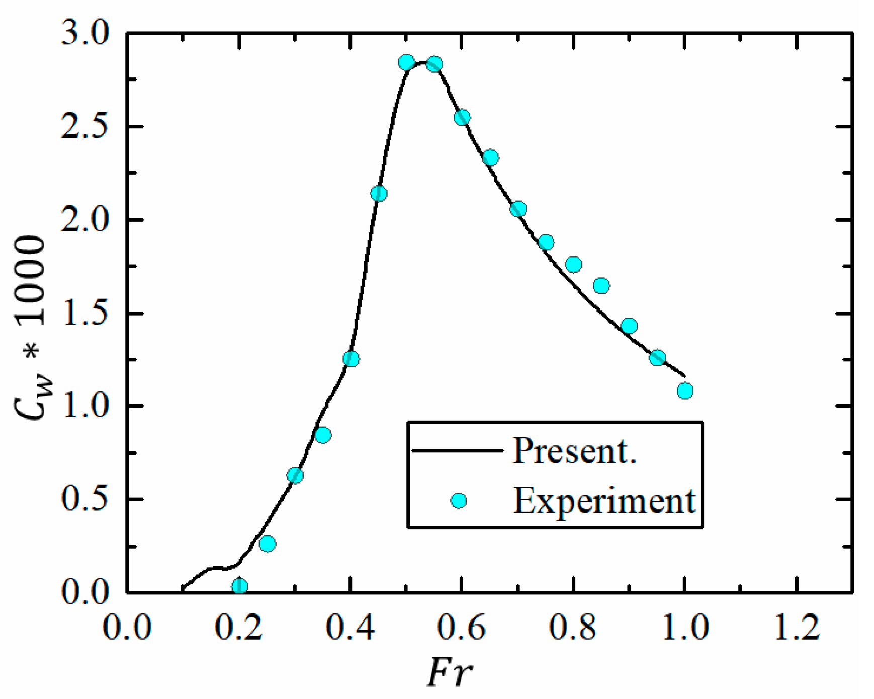
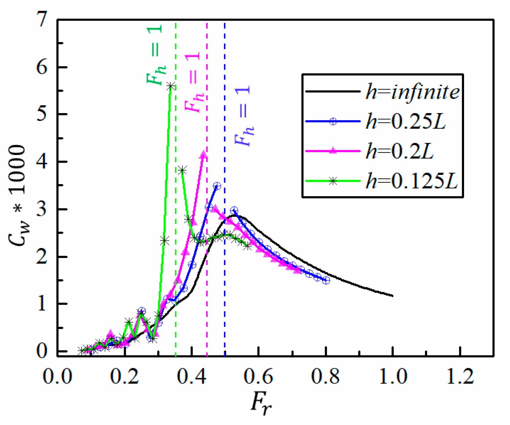
4.2.1. Wave-Making Resistance

Figure 7 shows the calculated wave-making resistance with respect to Froude numbers in different water depths. It can be seen in Figure 7 that the influence of water depth on wave-making resistances is not obvious at a low forward speed such as Fr < 0.3; after that, the curves in shallow water show a similar trend as that in deep water, but generally, the peak values shift toward the low forward speed. In addition, a dramatic increase of solutions can be witnessed near the transcritical speed F_h = 1.0 in shallow waters, and the reason is that the ship speed equals the maximum propagation velocity of gravity waves which then leads to a large accumulation of wave energy. However, the values around the F_h = 1.0 are omitted in this study since the convergent results are unable to be obtained, and the reason can be attributed to the invalid radiation condition because the wave propagates ahead of the ship in such a case.

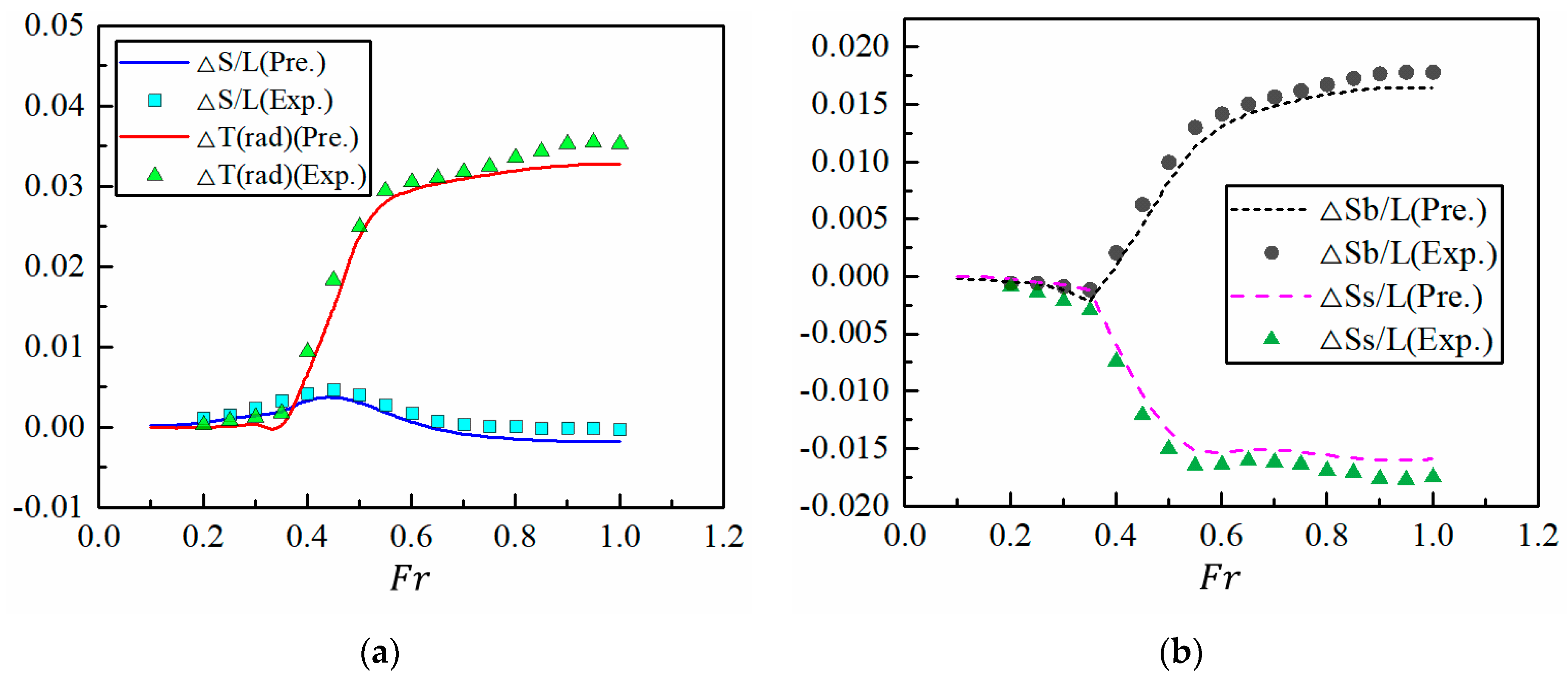
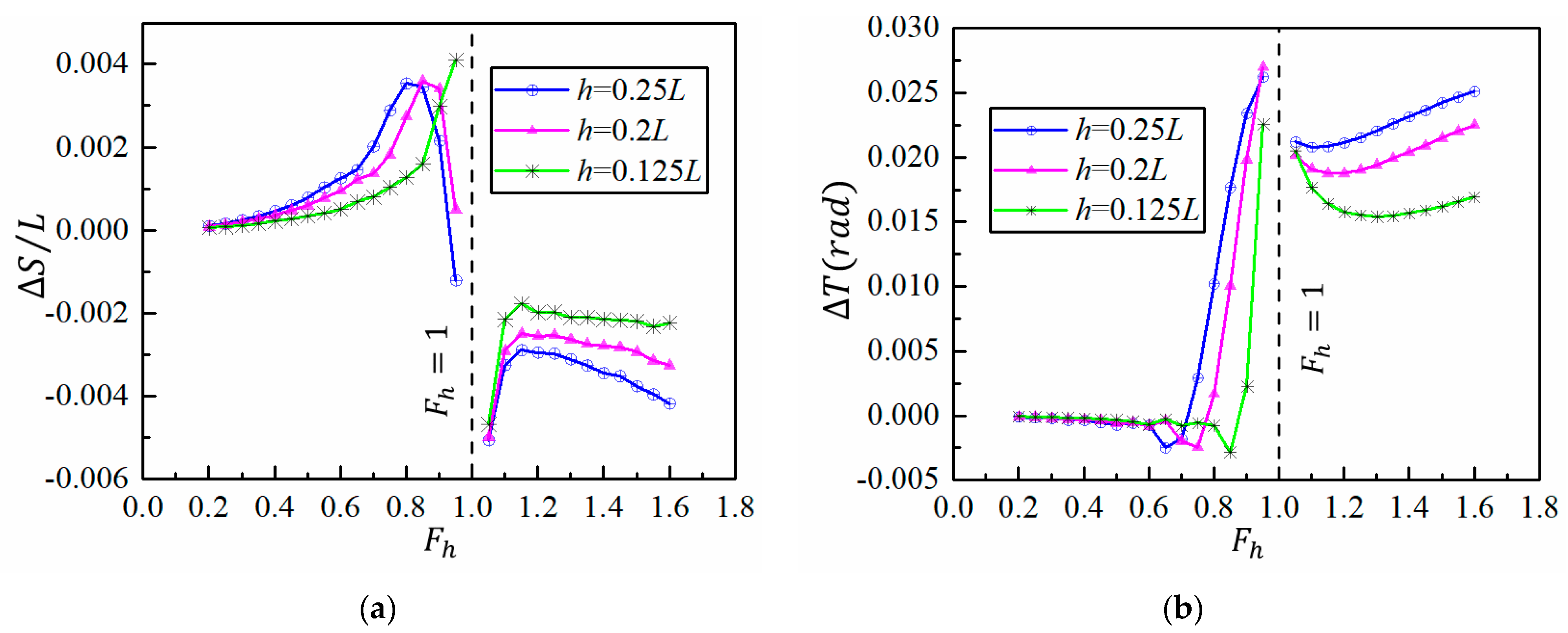
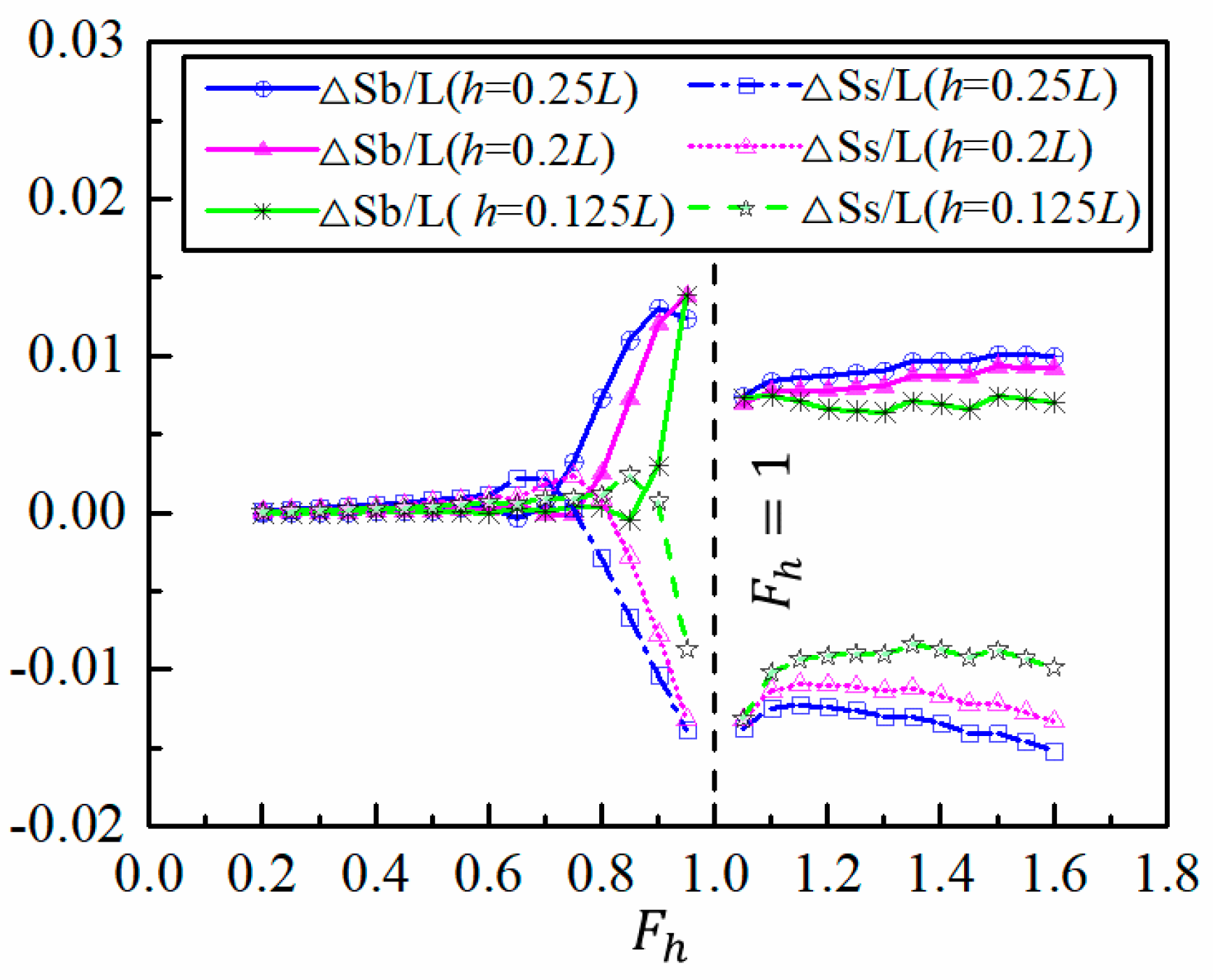
4.2.2. Sinkage and Trim

Figure 8 presents the comparisons of midship sinkage and trim for an NPL-4a ship at water depths h/L = 0.25, 0.2, 0.125. As can be seen in Figure 8a, peak values are obtained at subcritical range when F_h < 1.0, and then the curves experience a dramatic drop around the transcritical speed; after the transition point, F_h = 1.0, the results begin to decrease at supercritical speed F_h > 1.0. A similar trend can also be found for the trim solutions in Figure 8b and the dynamic sinkage of the bow and stern in Figure 9, which both show a crest value at the transcritical speed. This is because when the transcritical speed is reached, the transverse wave will combine with the diverging wave, which will cause a large increased sinkage and trim.

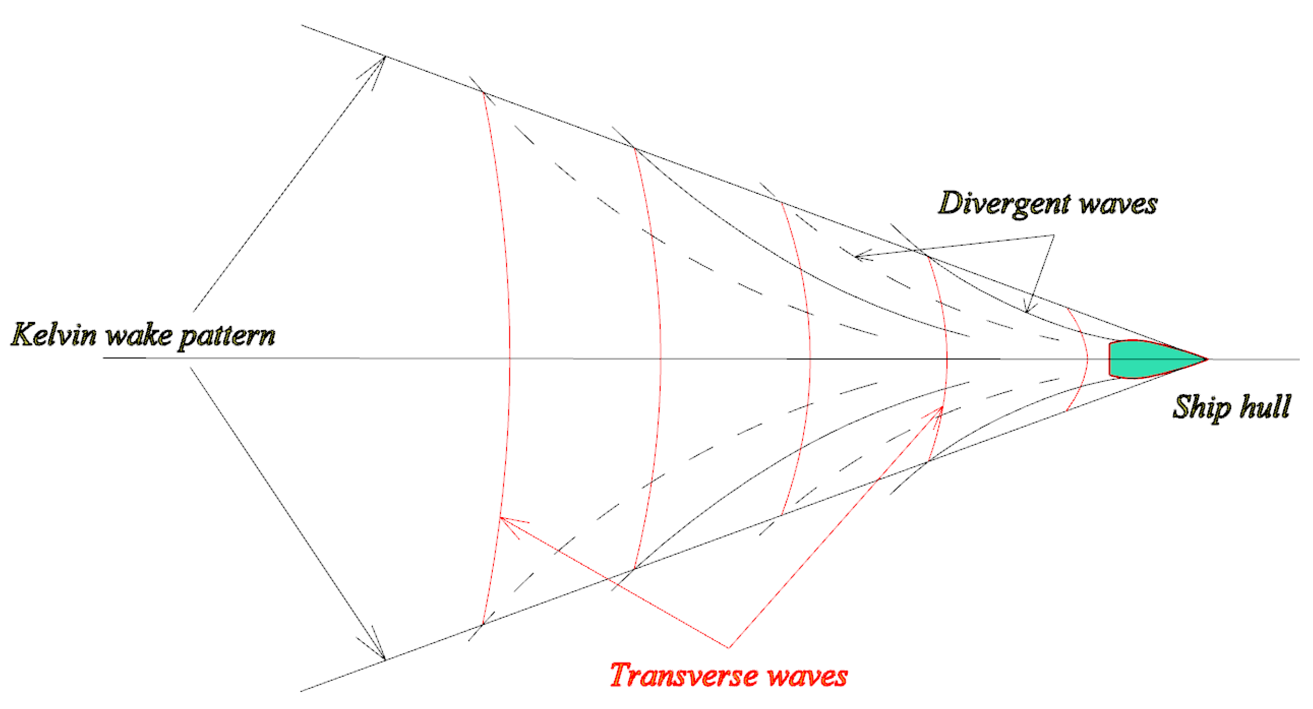
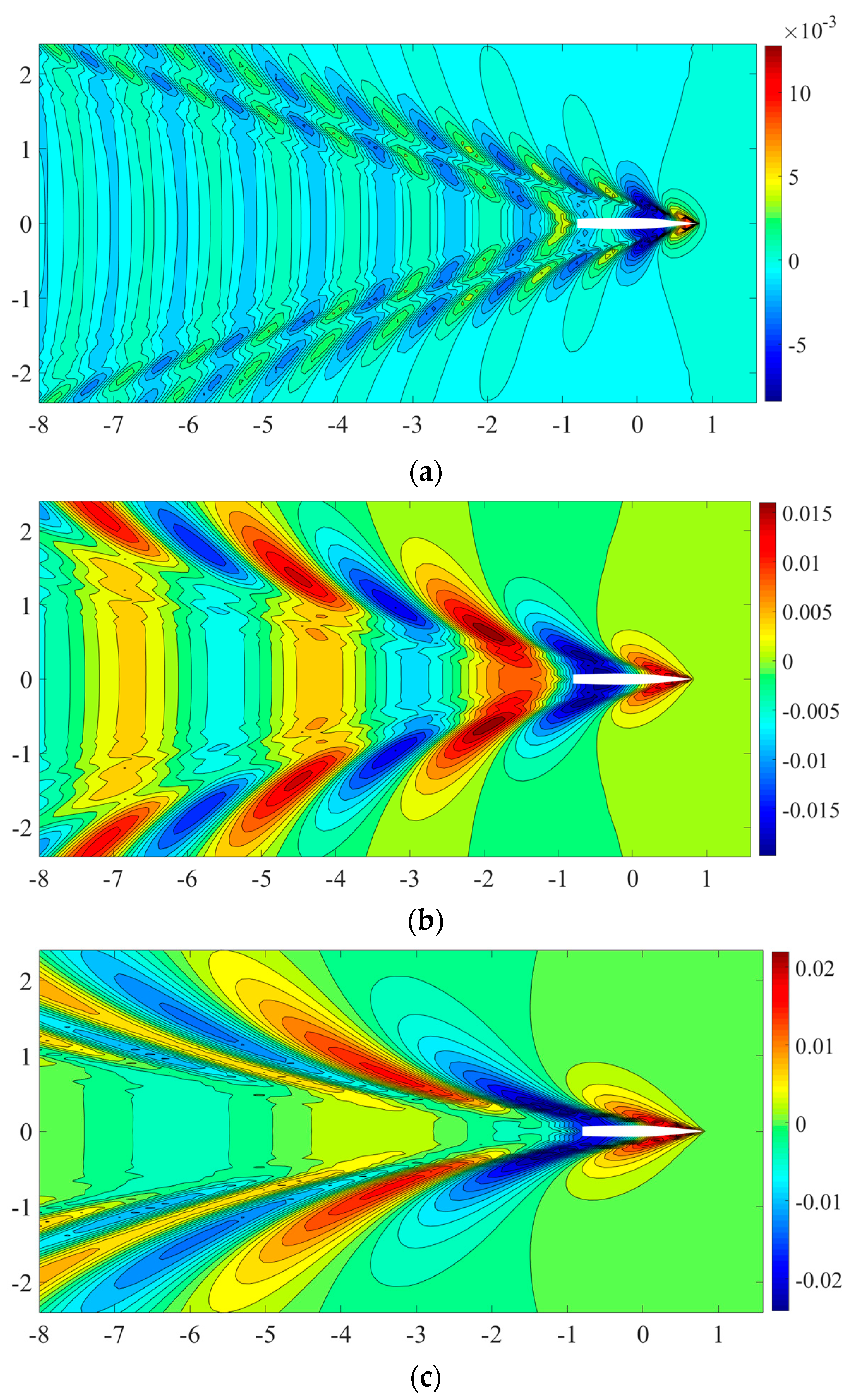
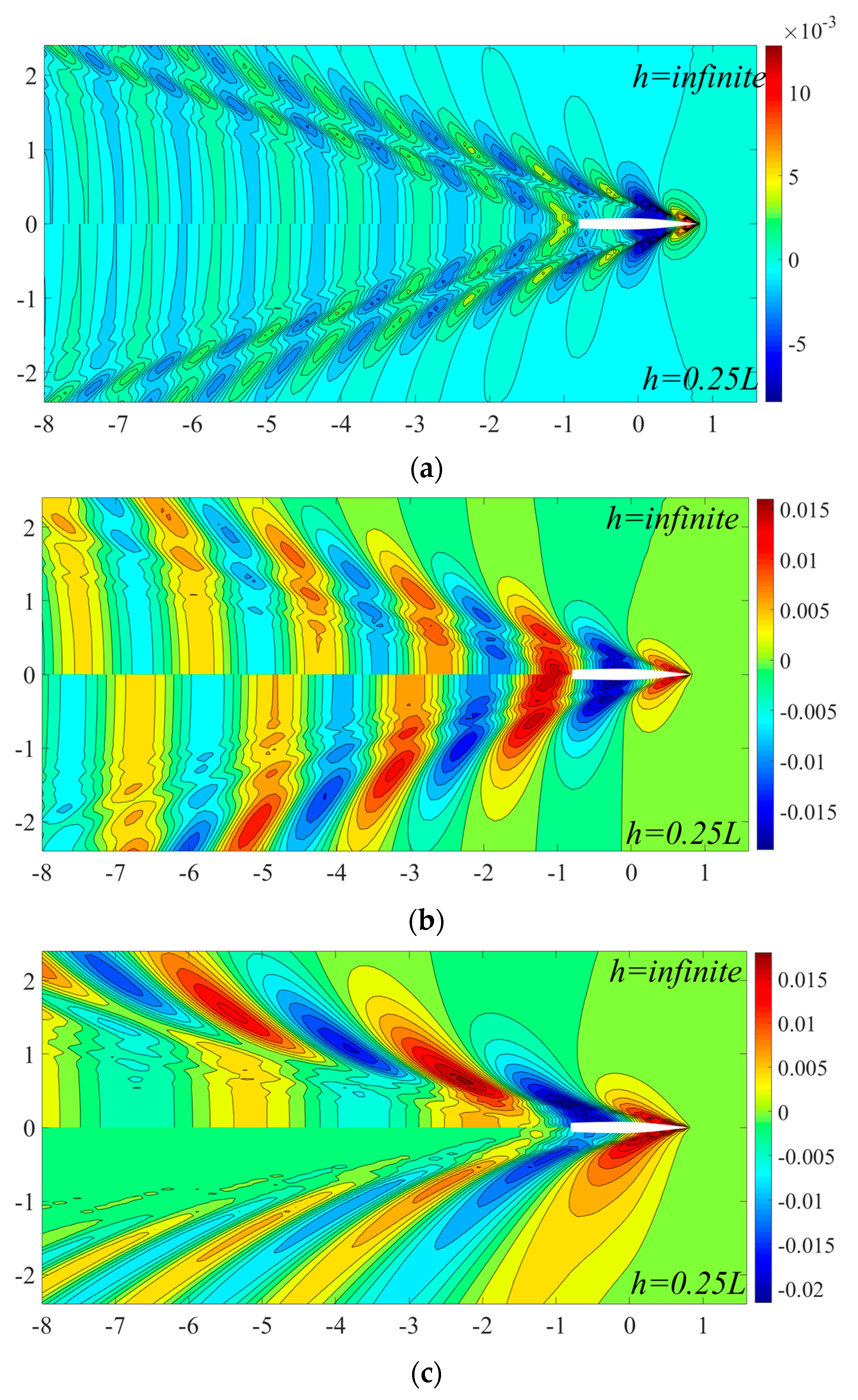
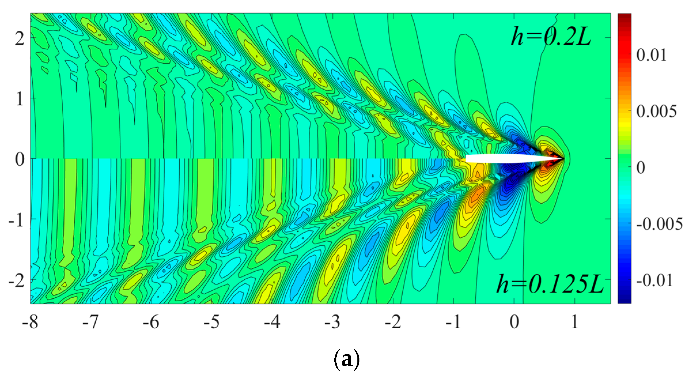
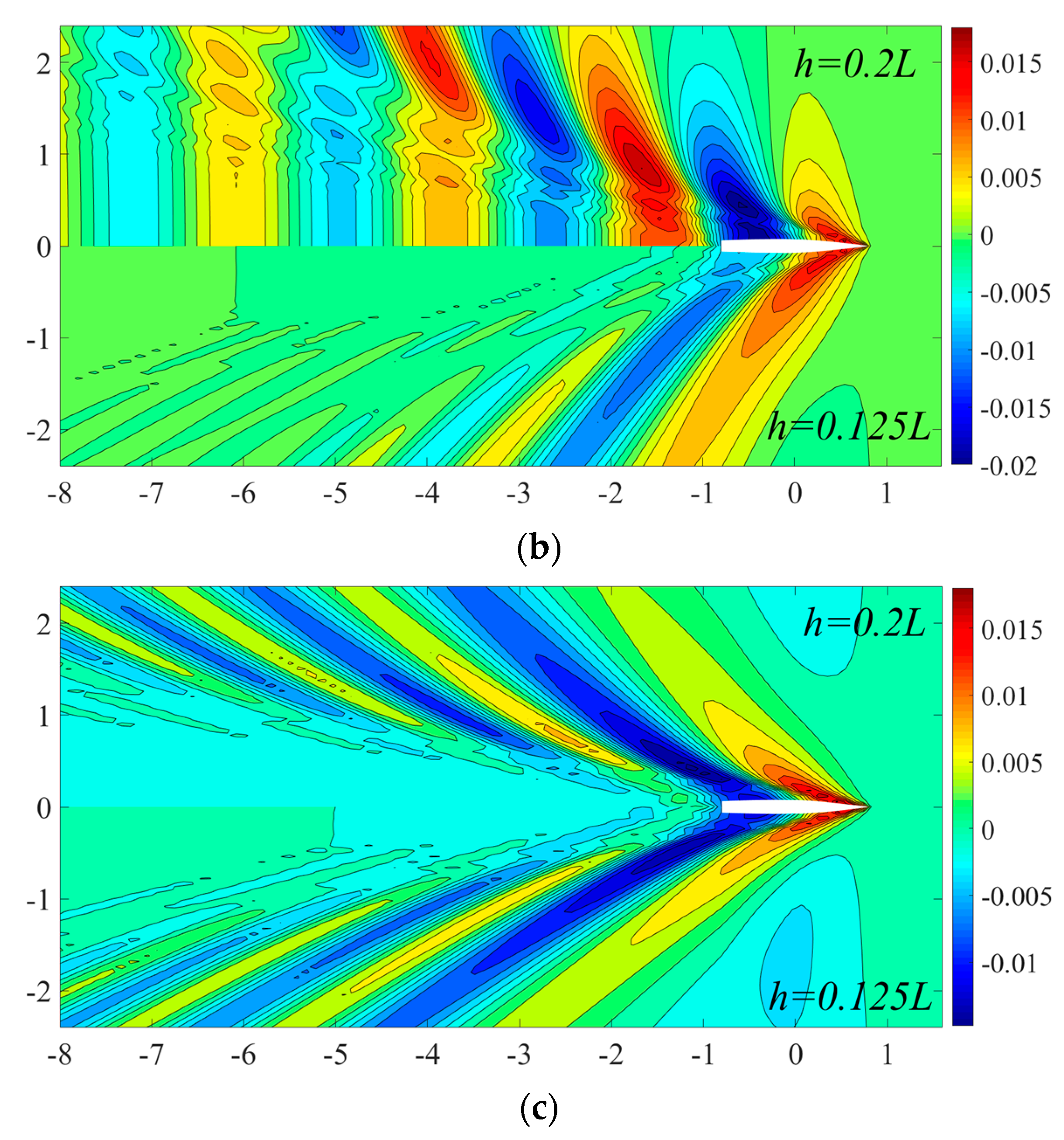
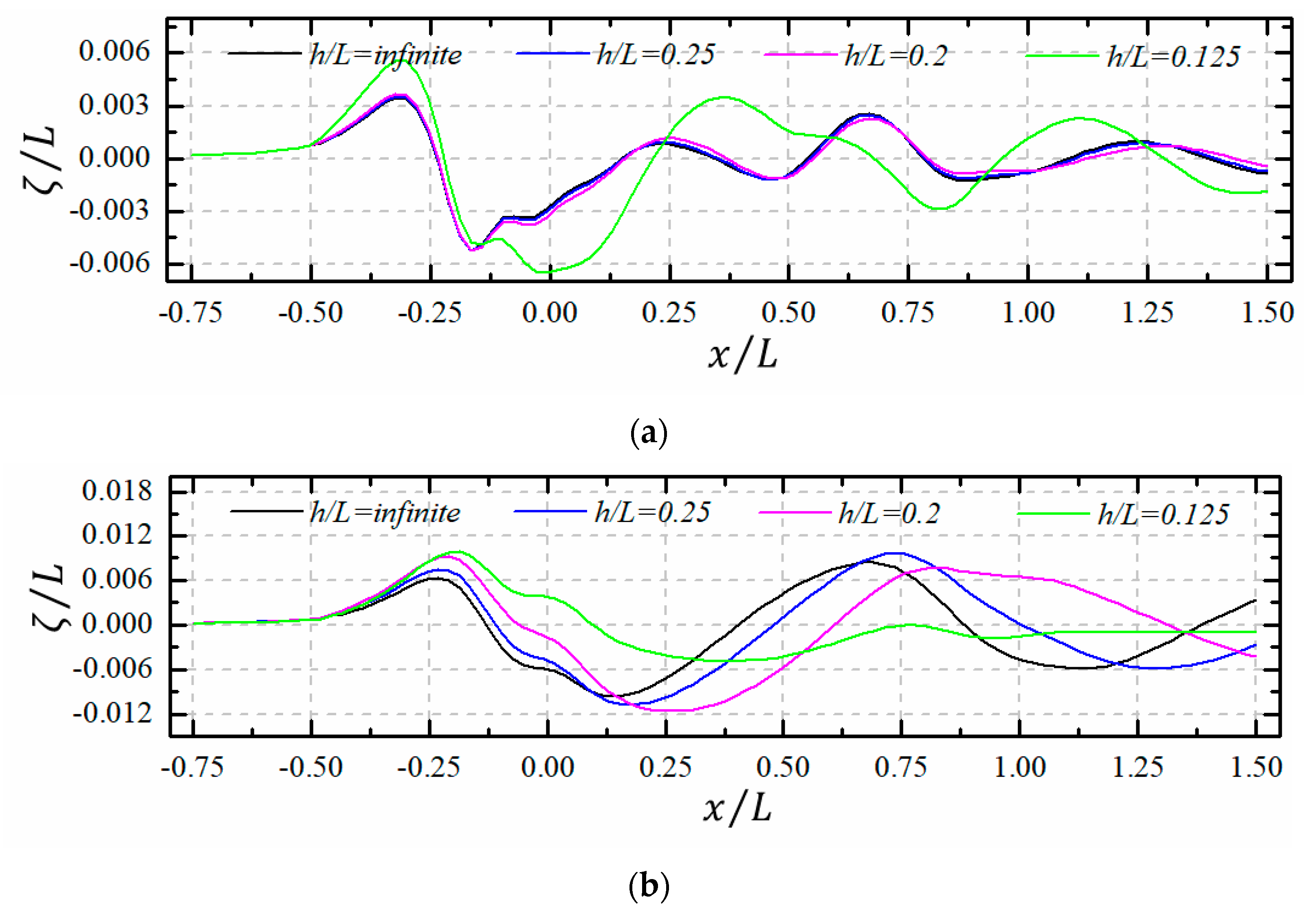
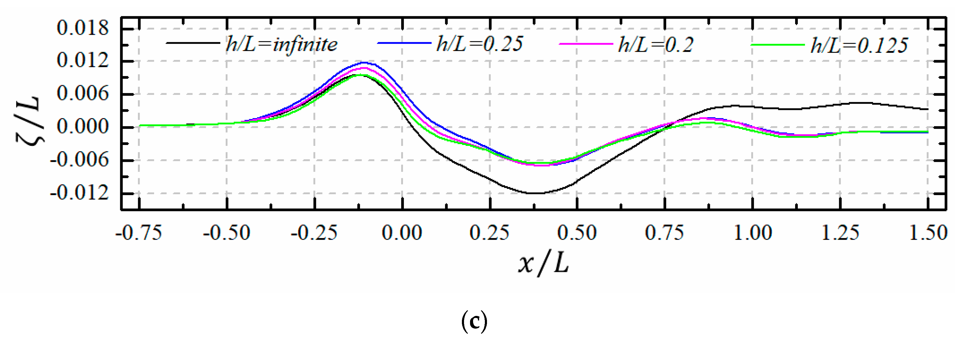
4.2.3. Wave Contour and Wave Profile

Figure 10, Figure 11 and Figure 12 illustrate the comparisons of wave patterns for NPL-4a ship moving at different speeds (Fr = 0.3, 0.4, 0.55) in different water depths (h/L = infinite, 0.25, 0.2, 0.125), where the corresponding water depth Froude numbers are also presented. As we can see from the figures, both the transverse waves and diverging waves exist at subcritical speed F_h < 1.0 in Figure 10a,b, Figure 11a,b, Figure 12a,b, while the diverging wave becomes the dominant component when supercritical speed F_h > 1.0 in Figure 10c, Figure 11c, Figure 12c; the physical phenomena give a reasonable explanation for the quick decrease of sinkage, trim and wave-making resistance when F_h exceeds the critical value 1.0. Moreover, the Kelvin angle increases as the water depth decreases, and will reach a maximum value of 90 degrees at F_h = 1.0 as demonstrated in Algie et al. [16]; however, the critical wave pattern is not shown here since the flow is not more of a steady state and the solitary waves are also generated.

Figure 13 gives the wave cuts at a transverse distance of 0.1L from the centerline for the NPL-4a ship moving in different water depths (h/L = infinite, 0.25, 0.2, 0.125). It can be seen from Figure 13a that the wave profiles do not show obvious differences at relatively low forward speed Fr = 0.3 in intermediate water depths, but the larger peak values are obtained when the ship moves in a risky water depth at h/L = 0.125. By comparing Figure 13a and Figure 13b, we can find that the peak values will increase with respect to the increased speed at subcritical speed F_h < 1.0; however, once the speed exceeds the transcritical speed F_h = 1.0, see in Figure 13c, the values in shallow water do not show large difference. Moreover, the peak values in shallow water are even lower than those in deep water behind the midship.

Table 4. The maximum and minimum values of the profiles at different forward speed in shallow water.

$\mathit{\zeta }/\mathit{L}$	Fr	h/L = Infinite		h/L = 0.25		h/L = 0.2		h/L = 0.125
		Value	$\mathit{x}/\mathit{L}$	Value	$\mathit{x}/\mathit{L}$	Value	$\mathit{x}/\mathit{L}$	Value	$\mathit{x}/\mathit{L}$
Maximum	0.3	0.00344	−0.3225	0.00352	−0.3225	0.0037	−0.3225	0.00555	−0.3225
	0.4	0.00837	0.6900	0.00963	0.7350	0.00918	−0.2100	0.00985	−0.1875
	0.55	0.0096	−0.1200	0.01176	−0.0975	0.01071	−0.1200	0.00951	−0.1200
Minimum	0.3	−0.00522	−0.1650	−0.00524	−0.1650	−0.00526	−0.1650	−0.0065	−0.0075
	0.4	−0.00959	0.1500	−0.01075	0.1725	−0.01161	0.2625	−0.00486	0.3750
	0.55	−0.01207	0.3750	−0.00697	0.3975	−0.00693	0.3975	−0.00659	0.3975

gives the maximum and minimum values of the profiles at different forward speeds in shallow water, and the corresponding positions of the extreme values are also listed in the table.

5. Conclusions

A Rankine HOBEM is developed for wave-making problems of a transom stern displacement ship moving in shallow water. By analyzing the computed results, the following conclusions can be drawn:

(1)

The computed results including wave-making resistance, singkage and trim in deep water show generally good agreement with test data, which demonstrates the stability and robustness of the present method. However, the errors at Fr ≤ 0.35 are larger than those in higher Fr, and the largest error even reaches about 75% compared with the experimental result in Fr = 0.2.

(2)

In general, the reduction of water depth results in a drastic increase of wave-making resistance, sinkage, trim and wave elevation, the values increase sharply near the transcritical water depth Froude number F_h = 1.0 due to the combining transverse wave and diverging wave, and after that the results begin to decrease as the evanescent transverse at supercritical speed. However, when a ship advances at supercritical speed in shallow water, the wave-making resistance may even be smaller than that in deep water.

(3)

Near the transcritical water depth Froude number F_h = 1.0, the ship will experience a dramatically increased sinkage and trim, which implies that the forward speed should be restricted to avoid grounding.

Though the nonlinear free surface condition is considered by adopting the iterative approach, the body surface condition is still satisfied on the mean wetted hull surface, and the accuracy may be improved by taking into account the hull mesh under the actual wave surface during iterations. This will be our future work.

References

1. Lataire, E.; Vantorre, M.; Delefortrie, G. A prediction method for squat in restricted and unrestricted rectangular fairways. Ocean Eng. 2012, 55, 71–80. [Google Scholar] [CrossRef]
2. Toxopeus, S.L.; Simonsen, C.D.; Guilmineau, E.; Visonneau, M.; Xing, T.; Stern, F. Investigation of water depth and basin wall effects on KVLCC2 in manoeuvring motion using viscous-flow calculations. J. Mar. Sci. Technol. 2013, 18, 471–496. [Google Scholar] [CrossRef]
3. Castiglione, T.; He, W.; Stern, F.; Bova, S. URANS simulations of catamaran interference in shallow water. J. Mar. Sci. Technol. 2014, 19, 33–51. [Google Scholar] [CrossRef]
4. Mucha, P.; Deng, G.; Gourlay, T.; el Moctar, O. Validation studies on numerical prediction of ship squat and resistance in shallow water. In Proceedings of the 4th MASHCON-International Conference on Ship Manoeuvring in Shallow and Confined Water with Special Focus on Ship Bottom Interaction, Hamburg, Germany, 23–25 May 2016; pp. 122–133. [Google Scholar]
5. Terziev, M.; Tezdogan, T.; Oguz, E.; Gourlay, T.; Demirel, Y.K.; Incecik, A. Numerical investigation of the behaviour and performance of ships advancing through restricted shallow waters. J. Fluids Struct. 2018, 76, 185–215. [Google Scholar] [CrossRef]
6. Gourlay, T.P.; Tuck, E.O. The maximum sinkage of a ship. J. Ship Res. 2001, 45, 50–58. [Google Scholar] [CrossRef]
7. Scullen, D.C. Calculation of linear ship waves. ANZIAM J. 2010, 51, C316–C331. [Google Scholar] [CrossRef]
8. Dawson, C.W. A practical computer method for solving ship-wave problems. In Proceedings of the Second International Conference on Numerical Ship Hydrodynamics, Berkeley, CA, USA, 19–21 September 1977; pp. 30–38. [Google Scholar]
9. Yuan, Z.M.; Kellett, P. Numerical study on a KVLCC2 model advancing in shallow water. In Proceedings of the 9th International Workshop on Ship and Marine Hydrodynamics, Glasgow, UK, 26–28 August 2015. [Google Scholar]
10. Yuan, Z.M. Ship hydrodynamics in confined waterways. J. Ship Res. 2019, 63, 16–29. [Google Scholar] [CrossRef]
11. Yao, J.X.; Zou, Z.J. Calculation of ship squat in restricted waterways by using a 3D panel method. J. Hydrodyn. Ser. B 2010, 22, 489–494. [Google Scholar] [CrossRef]
12. McTaggart, K. Ship squat prediction using a potential flow Rankine source method. Ocean Eng. 2018, 148, 234–246. [Google Scholar] [CrossRef]
13. Raven, H.C. A Solution Method for the Nonlinear Ship Wave Resistance Problem. Ph.D. Thesis, Delft University of Technology, Delft, The Netherlands, 1996. [Google Scholar]
14. Raven, H.C. Numerical wash prediction using a free-surface panel code. In Proceedings of the RINA Symposium Hydrodynamics of High-Speed Craft: Wake Wash and Motions Control, London, UK, 7–8 November 2000; ISBN 0 903055 62 7. [Google Scholar]
15. He, G.H. An iterative Rankine BEM for wave-making analysis of submerged and surfacepiercing bodies in finite water depth. J. Hydrodyn. 2013, 25, 839–847. [Google Scholar] [CrossRef]
16. Algie, C.; Gourlay, T.; Lazauskas, L.; Raven, H.C. Application of potential flow methods to fast displacement ships at transcritical speeds in shallow water. Appl. Ocean Res. 2018, 71, 11–19. [Google Scholar] [CrossRef]
17. Nakos, D.E.; Sclavounos, P.D. Kelvin wakes and wave resistance of cruiser-and transom-stern ships. J. Ship Res. 1994, 38, 9–29. [Google Scholar] [CrossRef]
18. Gao, G. Numerical implementation of transom conditions for high-speed displacement ships. J. Ship Mech. 2006, 10, 1–9. [Google Scholar]
19. Jensen, G.; Mi, Z.X.; Söding, H. Rankine source methods for numerical solutions of steady wave resistance problem. In Proceedings of the 16th Symposium on Naval Hydrodynamics, Berkeley, CA, USA, 13–18 July 1986. [Google Scholar]
20. Molland, A.F.; Wellicome, J.F.; Couser, P.R. Resistance Experiments on a Systematic Series of High Speed Displacement Catamaran Forms: Variation of Length-Displacement Ratio and Breadth-Draught Ratio; Ship Science Report 71; University of Southampton: Southampton, UK, 1994. [Google Scholar]
Figure 1. Body plan of NPL-4a ship model.
Jmse 12 00867 g001
Figure 2. Mesh discretization on ship hull and free surface.
Jmse 12 00867 g002
Figure 3. Comparisons of wave-making resistance coefficient for NPL-4a ship in deep water.
Jmse 12 00867 g003
Figure 4. Comparisons of sinkage and trim in deep water. (a) Midship sinkage and trim; (b) bow and stern sinkage.
Jmse 12 00867 g004
Figure 5. Kelvin wake pattern of transverse and divergent waves.
Jmse 12 00867 g005
Figure 6. Wave patterns for NPL-4a ship at different speeds in deep water. (a) Fr = 0.3; (b) Fr = 0.5; (c) Fr = 0.7.
Jmse 12 00867 g006
Figure 7. Comparisons of wave-making resistance coefficient for NPL-4a ship in different water depths.
Jmse 12 00867 g007
Figure 8. Midship sinkage (a) and trim (b) for NPL-4a ship at water depths h/L = 0.25, 0.2, 0.125.
Jmse 12 00867 g008
Figure 9. Dynamic sinkage of bow and stern for NPL-4a ship at water depths h/L = 0.25, 0.2, 0.125.
Jmse 12 00867 g009
Figure 10. Comparisons of wave patterns at h = infinite (upper half) and h = 0.25L (lower half). (a) Fr = 0.3 (Fh = 0.6). (b) Fr = 0.4 (Fh = 0.8). (c) Fr = 0.55 (Fh = 1.1).
Jmse 12 00867 g010
Figure 11. Comparisons of wave patterns at h = 0.25L (upper half) and h = 0.2L (lower half). (a) Fr = 0.3 (Fh = 0.6). (b) Fr = 0.4 (Fh = 0.8). (c) Fr = 0.55 (Fh = 1.1).
Jmse 12 00867 g011
Figure 12. Comparisons of wave patterns at h = 0.2L (upper half) and h = 0.125L (lower half). (a) Fr = 0.3 (Fh = 0.6). (b) Fr = 0.4 (Fh = 0.8). (c) Fr = 0.55 (Fh = 1.1).
Jmse 12 00867 g012aJmse 12 00867 g012b
Figure 13. Wave profiles produced by NPL-4a ship at different forward speeds in shallow water at y/L = 0.1. (a) Fr = 0.3. (b) Fr = 0.4. (c) Fr = 0.55.
Jmse 12 00867 g013aJmse 12 00867 g013b