Abstract
Non-metallic armoured optoelectronic cable winch systems (NAOCWSs) play critical roles in facilitating signal transmission and powering subsea equipment. Due to the varying depths in these applications, deploying the entire cable length is unnecessary. However, the portion of the cable that remains coiled around the winch can generate an electromagnetic field, which may interfere with signal transmission and induce electromagnetic heating. This can lead to elevated temperatures within the system, affecting the cable’s lifespan. Consequently, this study examines the distributions of magnetic and temperature fields within the NAOCWS with different currents (10–30 A) and numbers of winding layers (1–10). Findings indicate that the magnetic flux density (MFD) changes periodically, and the period is closely related to the distance between the cables. At the centre of the cable, the flux density is minimum. Temperature distribution correlates with both current amplitude and the number of winding layers, where an increase in either parameter amplifies the temperature variance between the edge and intermediate cables within the same layer. The current does not affect the internal temperature distribution pattern. With the number of winding layers determined, the layer where the highest temperature of the system is located is well defined and does not vary with current.
1. Introduction
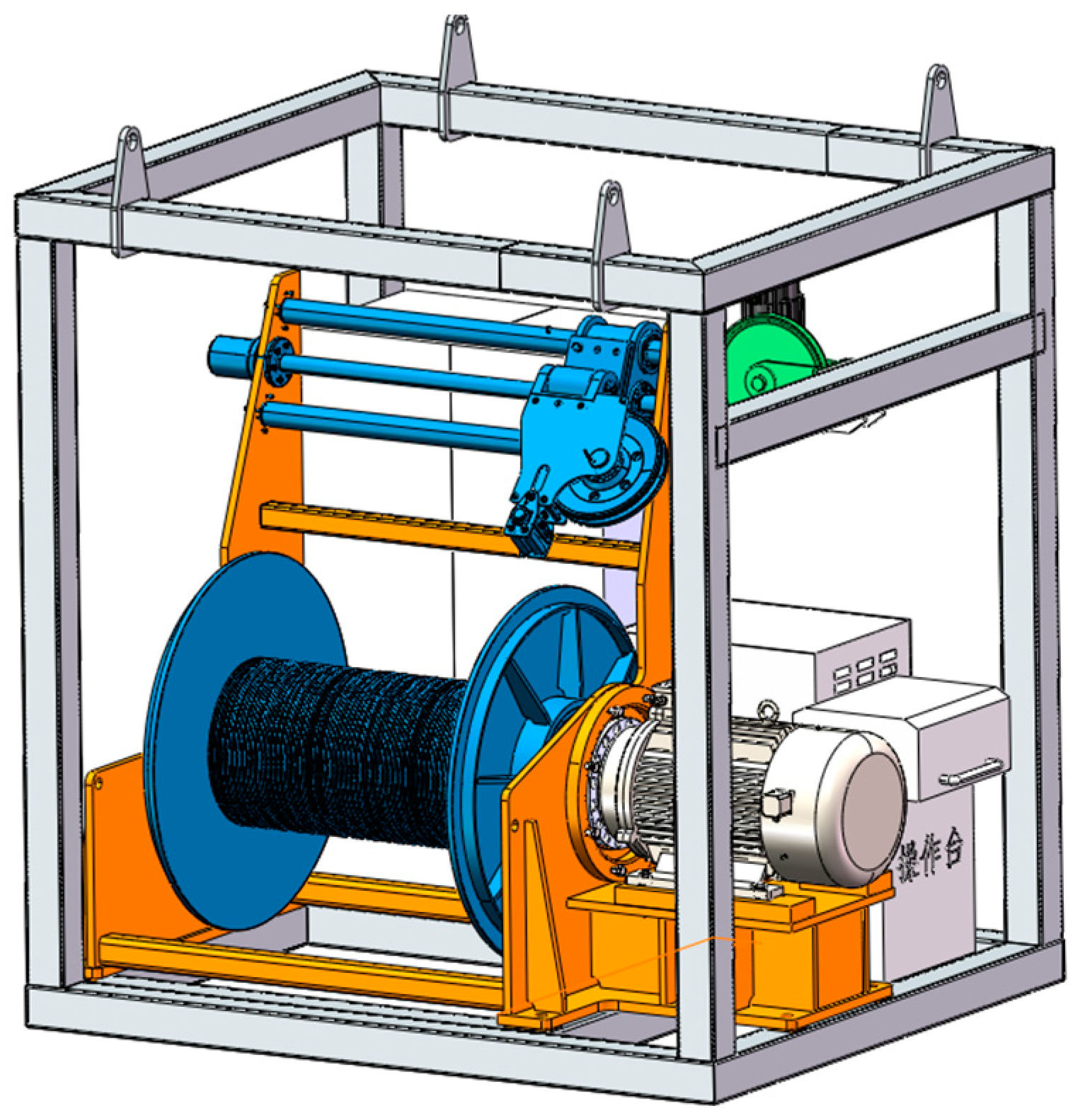
NAOCWSs are indispensable in marine exploration, acting as vital connectors and communication conduits between submersibles, exploration devices, towed bodies, other underwater operational tools and the mother ship, as depicted in Figure 1. Among their critical components, optoelectronic cables, available in metallic and non-metallic armoured versions, are paramount. Non-metallic armoured optoelectronic cables (NAOCs) are preferred for their superior strength-to-weight ratio, exceptional corrosion resistance [1,2] and adaptability to deeper marine environments and have been increasingly used in trace metal conductivity–temperature–depth (CTD) winches and remotely operated vehicle (ROV) winches in recent years [3].

Figure 1.
A non-metallic armoured optoelectronic cable winch system.
The elongation of cables required for deeper water operations introduces challenges, such as electromagnetic heating and signal interference due to magnetic fields, especially when cables are partially coiled on the winch, potentially compromising their longevity. This concern has prompted an increased research focus. Earlier studies, such as those by James R. Wait and Greg E. Bridges, have provided a precise formula for the electromagnetic field generated by underground cables, analysing the lossy electromagnetic field emanating from these cables [4,5,6]. Other researchers have employed 2D and 3D numerical simulations, predominantly using finite element methods, to delve into complex interactions [7,8,9]. For instance, Haoyan Xue conducted numerical simulations of the external electromagnetic fields of three-phase underground cables, analysing various factors affecting the fields [10]. Andrew summarized the electric and magnetic fields generated by cables in offshore wind farms, quantifying them through the finite element method (FEM), indicating that cables with excellent shielding properties do not directly produce electric fields outside the cable, yet they induce magnetic fields in the external environment [11]. Del-Pino-López utilized an ultra-shortened 3D-FEM model to investigate the magnetic field around such cables, offering insights into how cable material and design influence magnetic fields and proposing optimized designs [12].
Another issue that needs to be addressed urgently is temperature. Currently, NAOCs are primarily composed of cross-linked polyethene and an aramid armour. The insulation materials used in these cables can withstand a maximum heat-resistant operating temperature of 90 °C. Therefore, it is important to monitor the temperature closely. Traditional methods such as the equivalent thermal resistance approach, grounded in IEC 60287 standards, face limitations due to their reliance on simplified theories suitable only for uniform conditions and straightforward geometries [13,14]. In contrast, numerical solution methods, including boundary element, difference and finite element techniques, offer detailed simulations of actual conditions, enabling accurate analyses of coupled multi-physical fields. This approach, particularly through finite element analysis, has been shown to provide a more accurate assessment of cables’ current-carrying capacity and temperature profiles, surpassing the precision of conventional IEC calculations [15]. Research by Yunus Berat Demirol explored the thermal and electrical properties of parallel cable systems [16], while M. Rasoulpoor conducted thermal analyses considering load cycling and harmonic currents, suggesting adjustments for underground cable capacities [17]. S. Maximov developed an analytical model to evaluate cable gaps under varying underground temperatures [18]. N. M. Trufanova examined heat and mass transfer in rectangular ducts, considering electro-magneto-dynamic effects [19]. James Bangay compared thermal analysis methods from IEEE and CIGRE, exploring a hybrid model for reliability [20]. Weihua Chen devised a 900 m winch system for a multi-physics model integrating electromagnetic, fluid and temperature interactions, analysing temperature distributions and heat dissipation across different drum and cable layer configurations [21]. Ravichandran studied heat transfer in underwater umbilical cables on a winch, deriving safe bidirectional curves for various cable layers at specific environmental temperatures [22].
In summary, the current literature on electromagnetic heat in cables predominantly concentrates on the electromagnetic field of single or multiple cables arranged in parallel. There is comparatively limited research on the electromagnetic field of multi-layer entangled NAOCs, with only a few scholars having investigated NAOCs with fewer winding layers. Previous studies have not explored the distribution of magnetic fields and temperature within NAOCWSs. Therefore, the present work makes use of a multi-physics field coupling technique to examine how different currents and the number of winding layers affect the temperature distribution and MFD at various locations. This thesis aims to find the internal magnetic field distribution law, clarify the magnetic field distribution period and define the lowest position of the magnetic field inside the NAOC in order to provide a basis for the reasonable arrangement of signal lines inside the cable. At the same time, it explores the effect of the number of winding layers and current on the system interior to further clarify that the location of the maximum system temperature is independent of the current and is only related to the number of winding layers. It also gives the location of the highest system temperature in the case of windings of up to 10 layers. It provides a basis for the long-term stable, safe, economic and reasonable operation of NAOCWSs in engineering.
2. Mathematical Model
The analysis of optical cable winch systems involves a multi-physics field coupling problem. Theoretical and control equations of the electromagnetic thermal field are described during numerical simulation.
2.1. Electromagnetic Field Analysis of NAOCWS
When the NAOC is supplied with alternating current, the metal part of the cable generates eddy current loss due to the cable core and metal shield being subjected to an alternating magnetic field. On a macroscopic level, electromagnetic phenomena can be explained by the system of Maxwell’s equations [23]. Its essential variables include magnetic field strength H, electric field strength E, magnetic field density B and electric displacement vector D. The source variables include current density J and charge density ρ. As a result, Equation (1) represents Maxwell’s differential form for the electromagnetic field of the optoelectronic cable. In this article, we use bold letters for vectors.
where is vector differential operator, Je is the eddy current density and Js is current density. To characterize the macroscopic electromagnetic properties, one can express the parameters of Maxwell’s equations and the relationship between the relevant field quantities as shown in Equation (2):
where ε is the dielectric constant, μ is the magnetic permeability and σ is the conductivity. Combining Maxwell equations in a frequency domain, magnetic field intensity vectors can be defined as Equation (3) [24,25]:
where A represents the vector magnetic potential. Based on Maxwell’s equations, the vector magnetic potential equations for each layer of the cable are derived as shown in Equation (4) [26]:
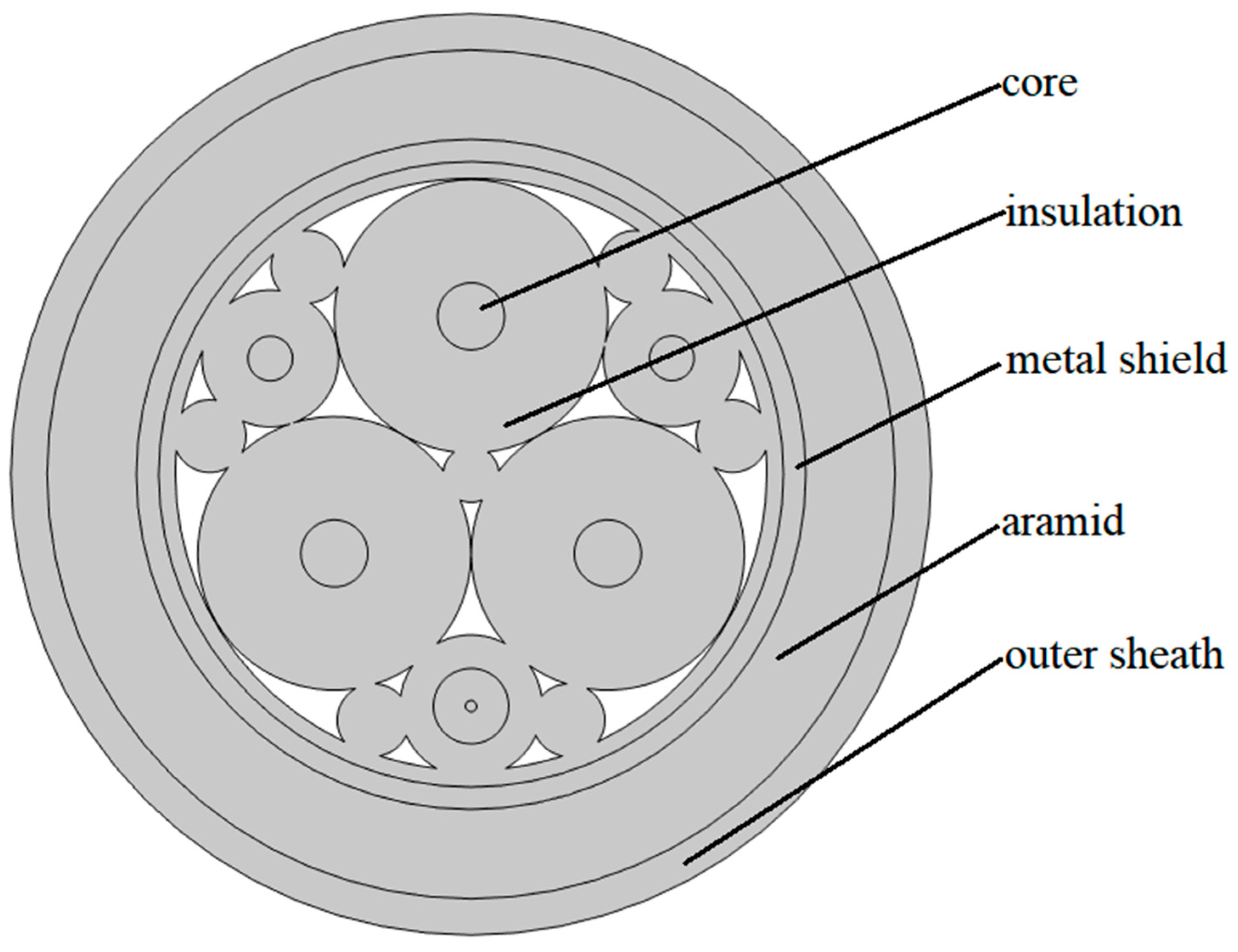
where represent the vector magnetic potentials of the cable’s core, insulation, metal shield, aramid and outer sheath, respectively, as shown in Figure 2.
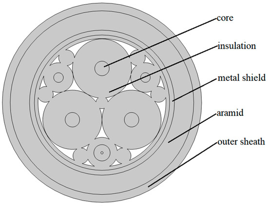
Figure 2.
Structure diagram of an NAOC.
The electro-magnetic-thermal multi-physics coupling model for an NAOCWS begins with the identification of the total heat source. In the process of heating and heat dissipation to equilibrium, control equations are used to describe the loading current in the conductor, heat transfer in fluids and solids, and electro-thermal coupling. The total heat sources of an NAOCWS include copper conductor current losses, metal shielding losses and insulation dielectric losses.
According to the international standard IEC 60287, the formula for copper core loss per unit length is shown in Equation (5) [27]:
where W1 is the resistance loss per unit length of the copper conductor, W/m; I is the load current of the copper conductor, A; R is the AC resistance per unit length at a given temperature, Ω/m; r is the DC resistance of the conductor core at a given temperature, Ω/m; ys is the skin effect coefficient; and yp is the proximity effect coefficient.
The DC resistance r of the conductor core is shown in Equation (6):
where r indicates the DC resistance per unit length of NAOC at T0 °C, Ω/m; r20 is the DC resistance of a copper conductor at 20 °C, Ω/m; and α is the temperature coefficient of resistance of the copper conductor; it is 0.37% here [28]. The conductivity of the copper conductor is shown in Equation (7):
where is the conductivity of copper, S/m; L is the length of the NAOC, m; and s is the cross-sectional area of the copper conductor, m2.
The skin effect coefficient and the proximity effect coefficient of the NAOC relationship are shown in Equations (8) and (9), respectively:
where f is the AC power supply frequency, Hz; and Ks is a constant, determined by the structure of the cable core; it is 1 here.
where dc is the outside diameter of the cable core; s is the distance between the centre axes of each cable core, m; and Kp is a constant, determined by the core structure of the cable; it is 0.8 here.
The currents in the three copper cores are shown in Equation (10):
where Ia, Ib and Ic represent the currents in the three conductors, respectively; I0 indicates the given current; and j is the imaginary unit.
Losses in the metal shield of the NAOC consist mainly of circulating current losses and eddy current losses. The metallic shield loss is obtained by calculating the ratio of the metallic sheath loss to the conductor loss of the NAOC, i.e., the metallic sheath loss factor λ1.
where represents the circulating current loss factor and represents the eddy current loss factor. Metal shield grounding inside an NAOC shows negligible loop current losses. The eddy current loss factor is shown in Equation (12) [29]:
where is the resistance of the metal shield at operating temperature, Ω/m; X is the reactance per unit length of the metal shield, Ω/m; s is the distance between the axes of the conductors, mm; d is the average diameter of the metal shield, mm; is the resistivity of the metal sheath, S/m; T′ is the working temperature of the shield, °C; AS is the ratio of shield temperature to conductor temperature; αs is the temperature coefficient of resistance of the shield, because the shield of a non-metallic armoured cable is copper, αs = α. Therefore, the metal shield loss is as shown in Equation (13):
The dielectric loss of NAOC insulation is shown in Equation (14) [30]:
where W3 is the dielectric loss power, W; ω = 2πf; f = 50 Hz; C0 is the capacitance of the NAOC per unit length, F/m; U0 is the phase voltage of the conductor, V; tanδ is the loss factor of insulation; is the dielectric constant of the insulating material; Di is the diameter of the insulating material, mm; and d1 is the diameter of the copper conductor, mm.
2.2. Heat Transfer Method for NAOCWS
When the NAOC is wound in multiple layers on a winch, heat primarily transfers through conduction between the cable and the winch. According to the law of conservation of energy, thermal energy is transported in non-metallic armoured cables between the inflow and outflow of a medium. This energy is transferred to the layers of the cable sequentially, achieving a balance within the cable’s medium, as shown in Equation (15):
where is the heat inflow from the system, is the heat outflow from the system, is the heat generated by the system and U is the increment of internal energy.
There are three basic modes of heat transfer in an NAOCWS: heat conduction, heat convection and heat radiation. This transfer occurs in the form of heat conduction, where thermal conductivity is dominated by heat transfer between solids. In these situations, the temperature field and current-carrying capability of the cable must be determined by coupling the two physical fields, the electromagnetic field and the temperature field. The process of heat conduction in a solid can be described by Fourier’s law, which applies to its microscopic elements. Additionally, it can be expressed by the law of conservation of energy and its continuity control equation. Heat conduction is the process by which heat moves through a medium from a hot spot to a cold spot as a result of a temperature differential. It is a fundamental heat transfer phenomenon [31]. According to Fourier’s law, the heat flow density q is directly proportional to the temperature change rate in that direction, as demonstrated in Equation (16):
where q is the heat flow density, W/m2; is the heat flux through area A′, W; and λ is the coefficient of thermal conductivity, W/(m∙K). The formula, also known as Fourier’s law, shows that the larger the λ, the better its thermal conductivity.
Thermal convection is the process of heat transfer between fluids or between the fluid and the solid when the fluid is in motion, and it is caused by a temperature difference between them. In the two-dimensional plane, the heat convection between air and the NAOCWS can be regarded as convection in a circular heat dissipation region. In order to determine the convection heat transfer coefficient, it is necessary to determine the state of the air flow. According to the Reynolds number, the state of air flow can be divided into three categories: laminar flow, transitional state and turbulent flow [32]. The Reynolds number Re for convective heat transfer in air is given by Equation (17):
where v, ρ′ and μ′ are the flow rate, density and viscosity coefficient of the air, respectively, and d is the characteristic length of the heat dissipation region. Because the heat dissipation area is circular, d is the diameter of the heat dissipation area.
If the air is turbulent, the process can be modelled through uniform out-of-plane convective losses [32].
where is the air’s mass flow rate; ; ρ is the density of air; v is the velocity of the air; A″ is the area of the heat dissipation area; is the air’s specific heat capacity; is the air’s intake temperature; T is the temperature of the system; V is the air’s volume, ; and r1 is the radius of the heat dissipation area.
Thermal radiation manifests as electromagnetic waves, which propagate through space. The quantity of heat emitted increases with the internal energy generated by higher temperatures. Unlike heat conduction and convection, thermal radiation transfers heat in the form of electromagnetic waves, even in a vacuum, without necessitating a medium [33]. The radiant energy that an idealized blackbody can absorb per unit time is shown in Equation (19):
where is the object’s area, β is the Stefan–Boltzmann constant and T′ is the object’s temperature. According to the formula, an object’s radiative capacity is directly related to the product of its temperature and surface area. When the temperature of a non-metallic armoured cable’s surface is and the surrounding air temperature is , heat is radiated between the cable and the air, as shown in Equation (20). The equation demonstrates the relationship between the two temperatures.
where is the emissivity of air and does not exceed 1.
The initial ambient temperature is set to 90 °C.
2.3. Evaluation of the Maximum Allowable Current-Carrying Ampacity of NAOCWS
The maximum allowable current-carrying ampacity (MACCA) is an important parameter of a cable. It refers to the insulation layer’s ability to withstand long-term operating temperatures without exceeding the insulation material’s temperature limit for the current. Therefore, the most immediate property that responds to the cable’s MACCA is the temperature of the core conductor. If the conductor current exceeds the current-carrying capacity of the cable for an extended period, the core temperature will exceed the temperature limit that the cable insulation materials can withstand. This will eventually cause damage to the cables by hastening the ageing process of the insulation layer material. Instead, cables are underutilized, resulting in resource charges. The cable’s temperature field and current-carrying capability must be precisely calculated in order to guarantee its long-term stability, safety and financially sensible functioning. The MACCA is restricted by the cable loss of heat in the temperature field of the inverse process of the solution, which involves multi-physics field calculations. This factor must be taken into account when calculating the solution process’s current-carrying ampacity [34]. The MACCA of the cable core is based on the number of stacked winding layers present when the temperature of the core exceeds the insulation withstand temperature of 90 °C for the long-term working life of the cable material. The solution is obtained using a numerical method; it draws its basis from the temperature field distribution results. The calculation is performed using the Secant method, whereby the solution process of the Secant method is illustrated in Equation (21):
where is the load current and is the cable’s maximum temperature at which the cable load current is . The MACCA calculation involves the following steps:
- The current is selected as and the maximum temperature of the cable at this moment is determined by using the finite element model. If the difference between and 90 °C falls within the permissible error, then represents the MACCA. Otherwise, proceed to step 2.
- If °C, then let ; otherwise, let . Use the finite element model to calculate the maximum temperature of the cable at this time. If the difference between and 90 °C falls within the permissible error, then represents the MACCA. Otherwise, proceed to step 3.
- Calculate using Equation (21) and through finite element modelling. If the difference between and 90 °C falls within the permissible error, then represents the MACCA. Otherwise, proceed to step 4.
- Let , , and , and proceed to step 3.
Based on the above theory, the following assumptions are made:
- The properties of all materials except copper are constant;
- Thermal convection and thermal radiation from the internal gaps of NAOCs are neglected;
- Charge density ρ and its effects can be neglected because the supply is 50 Hz;
- NAOC internal contact thermal resistance is neglected;
- Spiral windings are simplified to circular turns;
- Heat loss during thermal convection is simplified to uniform convection loss.
3. Convergence and Validation Studies
3.1. Evaluation of the MACCA of NAOCWS
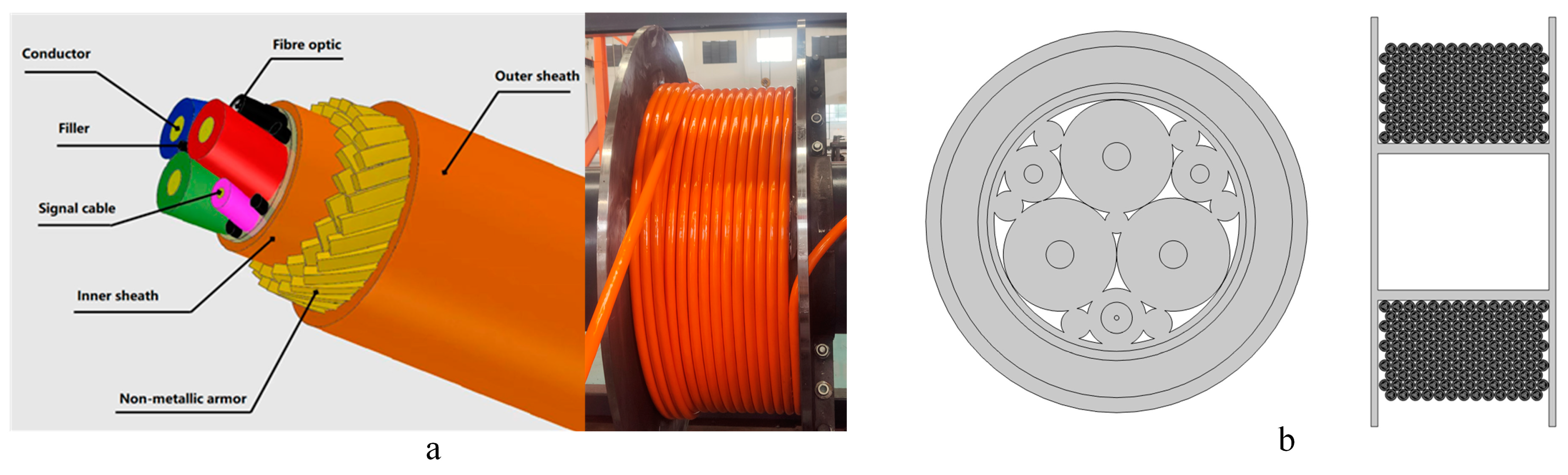
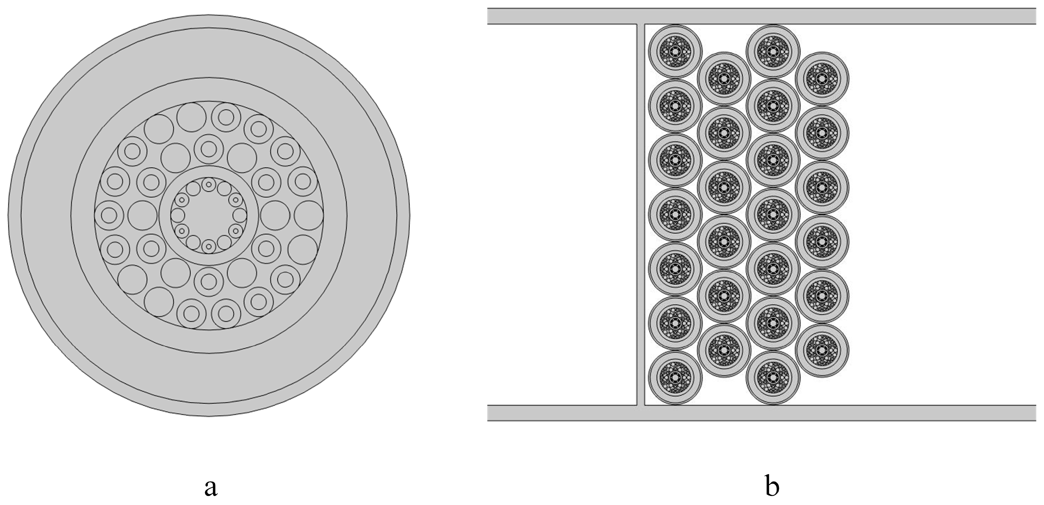
NAOCs are typically armoured with either aramid or cross-linked polyethene. This paper focuses on researching aramid-armoured optical cables. The cable is a three-core cable that consists mainly of copper core, optical fibre, insulation, inner sheath, metal shield and outer sheath. Its structure is illustrated in Figure 3a. To simplify the calculations, we chose a 2D axisymmetric model for numerically simulating the NAOCWS. The electromagnetic thermal solution model of the non-metallic optical cable winch system using COMSOL Multiphysics 6.1 software is shown in Figure 3b.
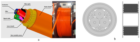
Figure 3.
NOACWS physical and simulation model: (a) physical model; (b) 2D axisymmetric simulation model.
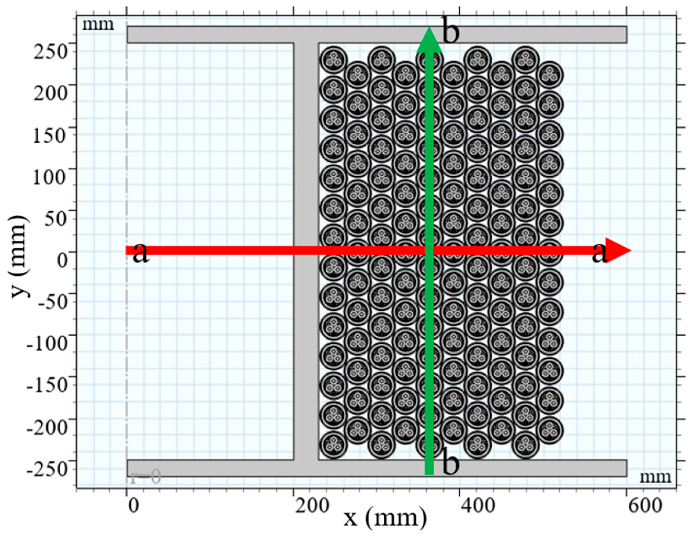
The paper presents numerical simulations of winches wound with 1–10 layers of an NAOC. Each layer contains either 13 or 14 turns of the NAOC. The upper cable is sandwiched between the two lower cables. The cable is internally energized with a 50 Hz alternating current. Under normal operation, the metal shield of the NAOC is typically safely grounded. Table 1 presents a detailed summary of the NAOCWS used in the calculation setup. The appropriate current load for copper cables is determined following IEC 60335-1: the copper core wire’s cross-sectional area is 4 mm2, and the maximum allowed long-term current ranges from 25 A to 32 A [35]. As a result, the range of 10 A to 30 A is the maximum value of current in the NAOC in this study. Meanwhile, this paper analyses the magnetic field strength, temperature results and distribution at the following locations. A two-dimensional coordinate plot of the NAOCWS is established, as shown in Figure 4, with the red line a–a indicating the radial direction along the winch and green line b–b indicating the position of the same layer of cable. This paper analyses the magnetic field and temperature distribution inside the system in two main directions.

Table 1.
The geometry of a non-metallic armoured optoelectronic cable and winch.
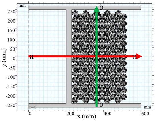
Figure 4.
Position in the NOACWS model.
As this paper involves coupling between electromagnetic and thermal fields, material selection and parameter values are set accordingly. The selection of materials for an NAOC includes a cable core, metal shielding material for copper, insulation material for cross-linked polyethene, and inner and outer sheaths for polyethene. The material properties and parameters are determined based on the corresponding material and the physical field applied, as shown in Table 2.
Table 2.
Specifications for materials for every layer of cable.
3.2. Cooling Area Selection
According to Table 1, the diameter of the NAOCWS is 600 mm, so the diameter of the heat dissipation area selected in the simulation software should be greater than 600 mm. In this paper, a wind speed of 0.1 m/s is chosen to take into account the calm sea level. Reynolds number >4000, so air flows in the heat dissipation area for turbulence. Initially, five types of cooling diameters were selected as cooling areas: 700 mm, 1400 mm, 2100 mm, 2800 mm and 3500 mm. As an illustrative example, consider a 10 A current and six-layer winding system. Table 3 presents the highest temperatures observed in the system under each cooling area. When the cooling area exceeds 2100 mm, the system’s maximum temperature area remains constant, so this article selects a 2100 mm cooling area.
Table 3.
Temperature in different cooling zones.
3.3. Meshing and Dependence Check
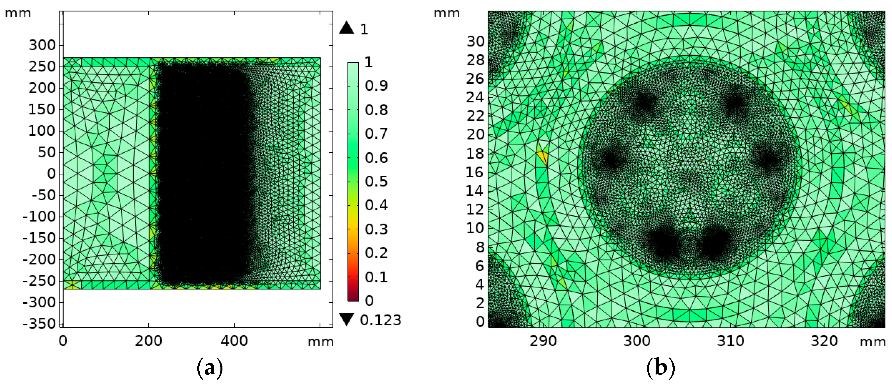
After determining the simulation theory, the accuracy of the numerical simulation results mainly relies on finite elements, mainly including the number of elements, quality and shape aspects. This study used COMSOL simulation software to perform mesh division on the electromagnetic thermal domain of the NAOCWS. As shown in Figure 5, the number of elements in the non-metallic armoured cable winch system is 8.7 × 10⁵, and the average mesh quality is 0.812, which meets the requirements. In numerical simulations, the number of meshes generally represents the accuracy of the simulation. However, increasing the number of meshes will increase the calculation time, while decreasing the number of meshes will reduce the calculation accuracy. Therefore, choosing an appropriate number of meshes for mesh independence verification to balance the relationship between calculation time and accuracy is necessary.
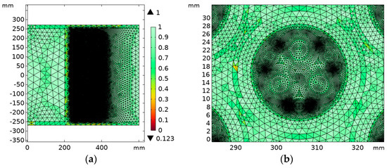
Figure 5.
Grid division: (a) overall grid division; (b) local grid division.
The 10 A current, six-layer winding case was selected as a representative for grid-independent validation. Four grid numbers, 4.3 × 10⁵, 8.7 × 10⁵, 1.18 × 10⁶ and 1.53 × 10⁶, were chosen to select the highest temperatures at four points in systems A (248, −232), B (−248, −90), C (−248, 52) and D (−248, 194), respectively. As shown in Table 4, the number of grids is 8.7 × 10⁵ and 1.18 × 10⁶ and the temperatures at each location are closest, but the computation time differs by a factor of 2. Accordingly, in this simulation study, the number of grid points is set to 8.7 × 10⁵ for all simulations.
Table 4.
Temperature at each location for different number of grids.
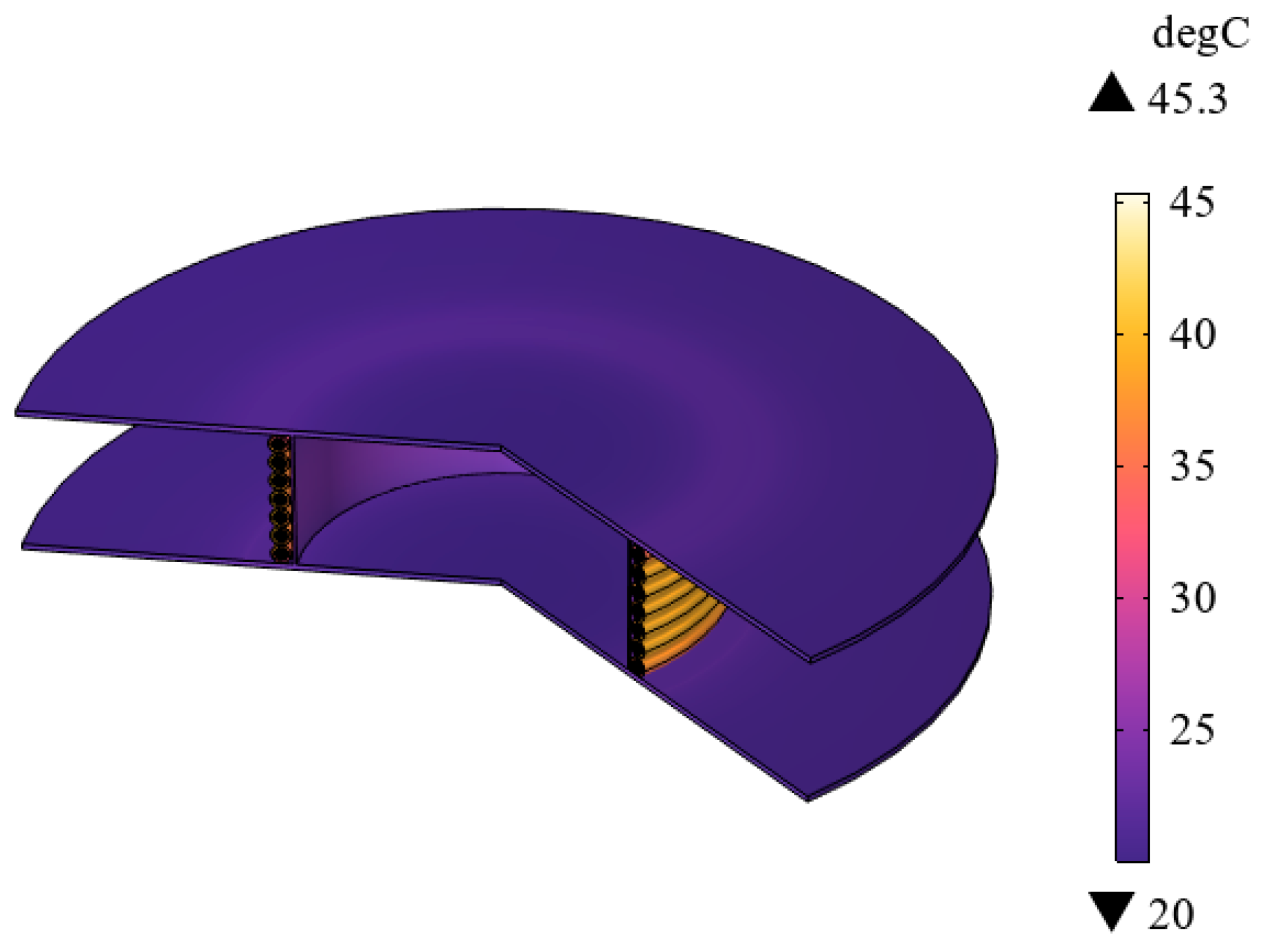
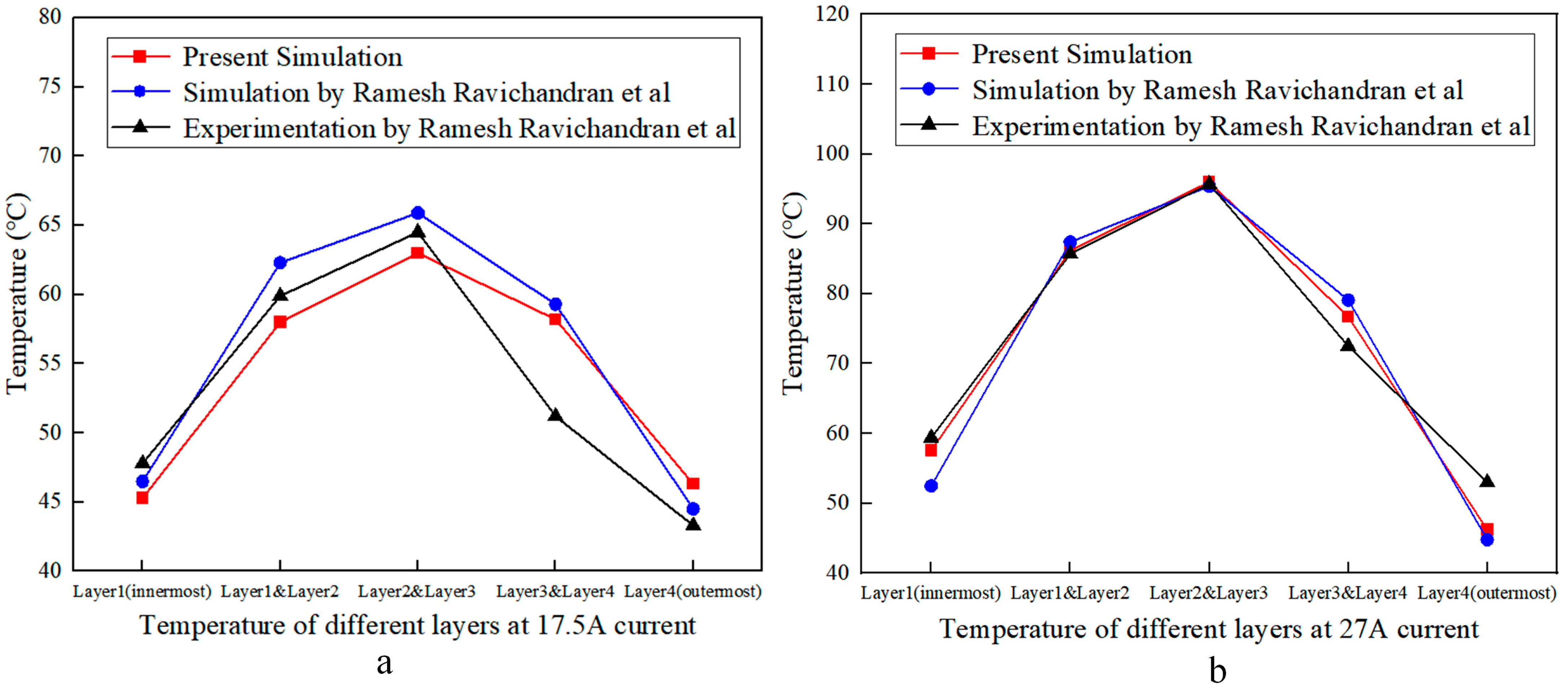
Ravichandran et al. investigated the heat transfer characteristics of underwater umbilical cables wound around winches [22]. This study employs an electromagnetic thermal multi-physics coupling approach to recreate the optical cable winch model presented in Ravichandran’s work, as illustrated in Figure 6. The accuracy of the numerical model and computational methods used in this research was confirmed through a detailed comparison with both the simulation and experimental results reported in their study. Figure 7 displays the highest temperature at the winch system and the first layer of the cable under a rated current of 17.5 A. Comparative analysis with the data from their publication revealed that under a rated current of 17.5 A with four layers of winding, the highest temperatures escalated from the first to the second layer and decreased from the third to the fourth layer, peaking between the second and third layers. This pattern was consistent even at a rated current of 27 A, as depicted in Figure 8. Accordingly, the numerical simulation methods employed herein accurately replicate the temperature dynamics of the non-metallic armoured optical cable winch system.

Figure 6.
Winch and cable model in the literature [22]: (a) cable model; (b) winch model.

Figure 7.
Temperature of the first layer at 17.5 A current.
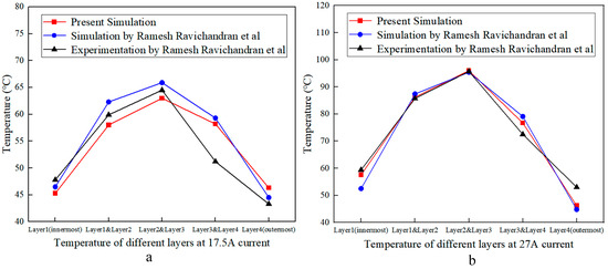
Figure 8.
Comparison of experimental and simulated data at different currents: (a) 17.5 A; (b) 27 A [23].
4. Results and Discussion
4.1. Effects of Current on Magnetic Fields
The NAOCWS is distinctly different from laid cables or tunnel cables. The structure comprises a single cable stacked and wound on the winch. When cables carry three-phase AC currents, the resulting magnetic fields interact. Changes in magnetic fields can significantly impact cable signal transmission. Therefore, it is crucial to comprehend the magnetic field’s magnitude and have efficient management over it in order to guarantee the system’s safety and dependability, as well as a clear identification of the current-to-magnetic field distribution and changes in the NAOCWS.
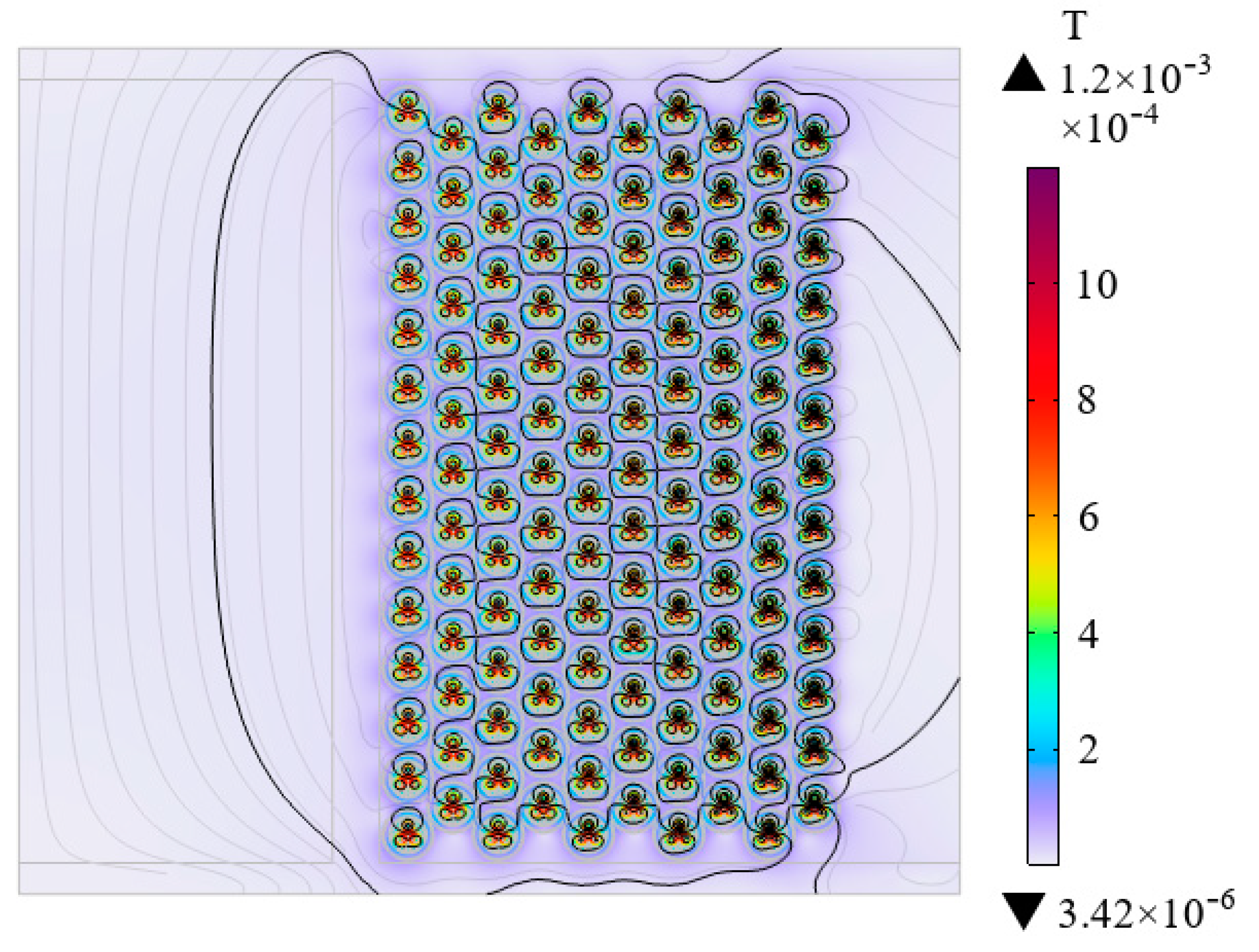
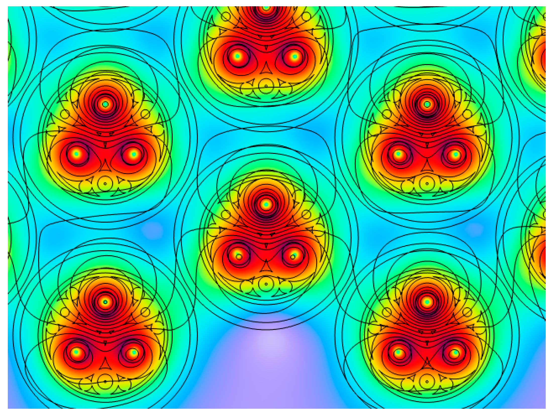
This section investigates the effect of current on the magnetic field in the NAOCWS using different amplitude currents (10 A, 15 A, 20 A, 25 A, 30 A) as examples. As shown in Table 5, the maximum MFD has a significant change with the increase of current when the optical cable is wound in multiple layers, and the increase is a constant value, indicating that the magnetic flux density is proportional to the current. At the same time, the maximum MFD in the system is analysed at different currents with 1, 4, 7 and 10 layers of winding, and its magnitude does not change, indicating that there is no relationship between the magnitude of the maximum magnetic flux density and the number of layers of winding. As illustrated in Figure 9, the isometric magnetic flux density diagram reveals a higher internal magnetic flux density in the non-metallic armoured areas compared to that of the winch, also highlighting a distinct spatial relationship. For enhanced visibility of the internal magnetic flux density, a localized enlargement is provided in Figure 10, showing that the interference of cables between different layers is small and that the distribution law of magnetic field strength between each cable is almost the same. Consequently, further investigation into the magnetic field intensity at various system locations will continue, aiming to elucidate a more definitive relationship between the current strength and the system’s internal magnetic fields.
Table 5.
Maximum magnetic flux density at different currents.

Figure 9.
Lines of equal magnetic flux density.
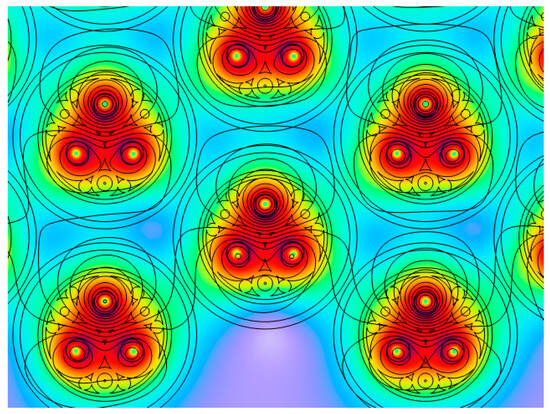
Figure 10.
Magnetic flux density localized magnification.
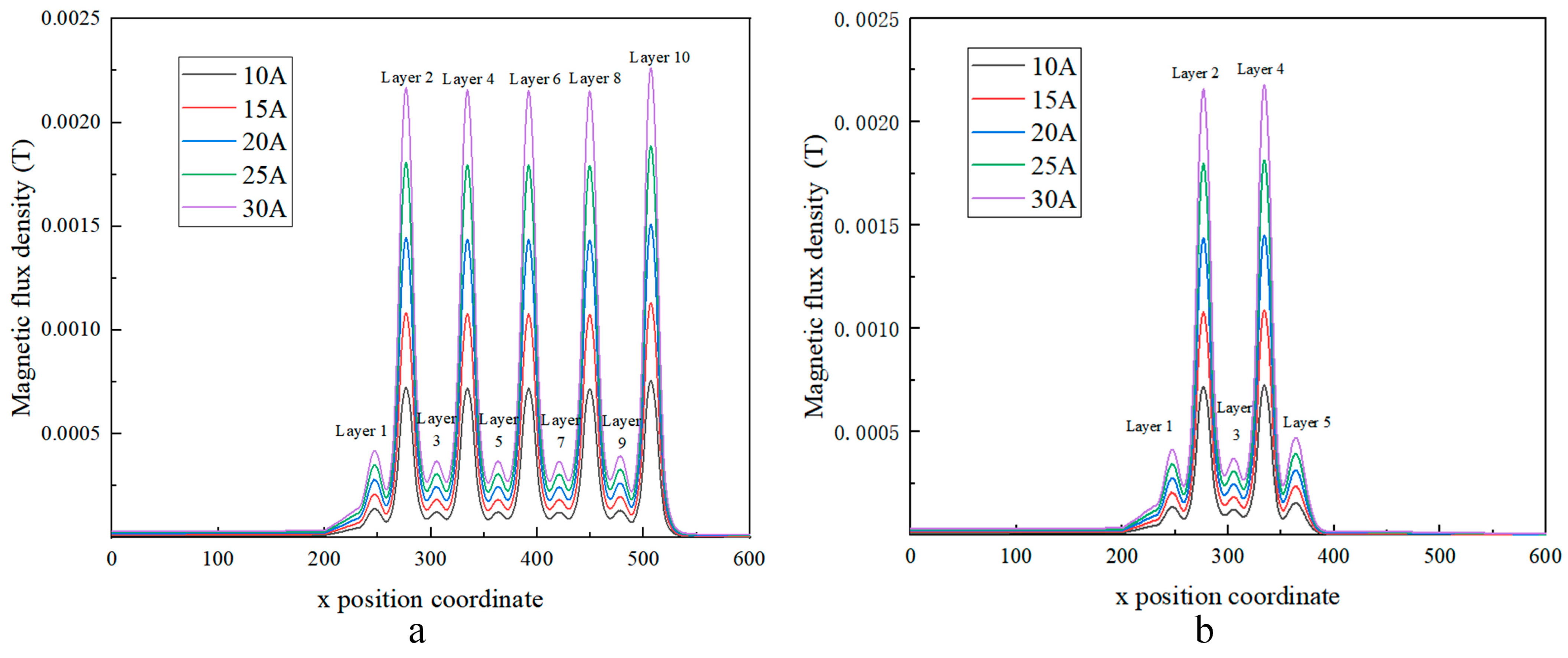
Analysed along the a–a direction as shown in Figure 3, it is clear that it passes between the two cables of the odd layers (specifically 1, 3, 5, 7 and 9) and through the centre of the cables of the even layers (specifically 2, 4, 6, 8 and 10). The analysis of the selected 10-layer winding case is shown in Figure 11a. The MFD exhibits periodic variation, with the period being the distance between the centre of the two layers of cables. The MFD between the two layers of cables is negligible, causing the positions to cancel each other out. Conversely, the MFD in the centre of the cables is significant, resulting in the positions reinforcing each other. There is a decrease followed by an increase in MFD along the axis from the lower to the higher layers of the winding. There are fewer NAOCs on the outside of layers 1 and 2, as well as layers 9 and 10. This better illustrates that the magnetic fields between the different layers weakly interfere with each other. The magnetic field distributions of the 5-layer and 10-layer windings were compared. The results show that the patterns are identical (Figure 11b).
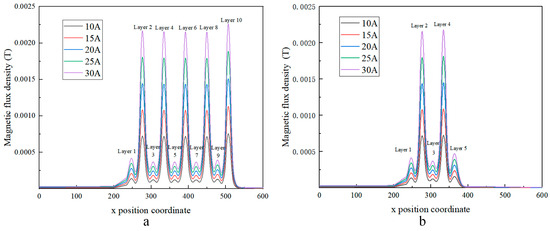
Figure 11.
MFD in the horizontal axis at different currents: (a) 10 layers; (b) 5 layers.
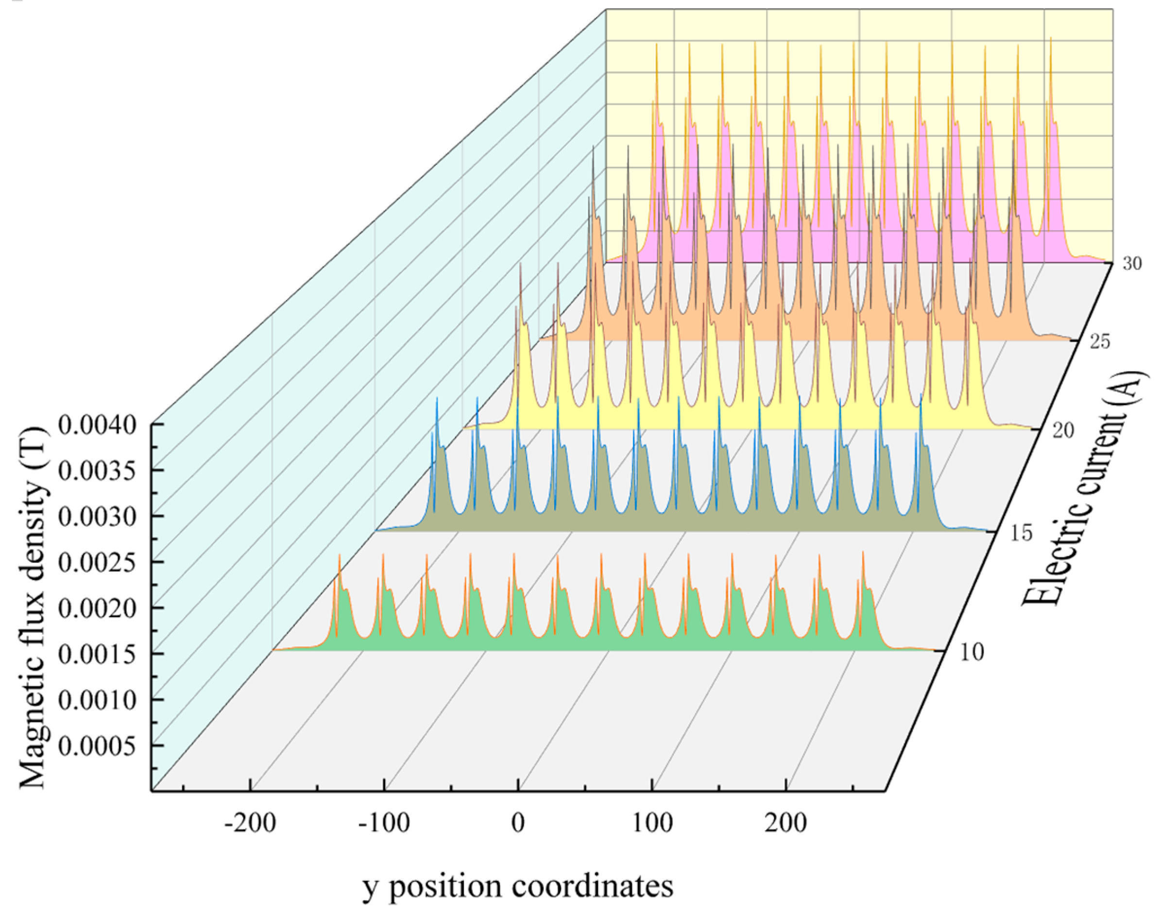
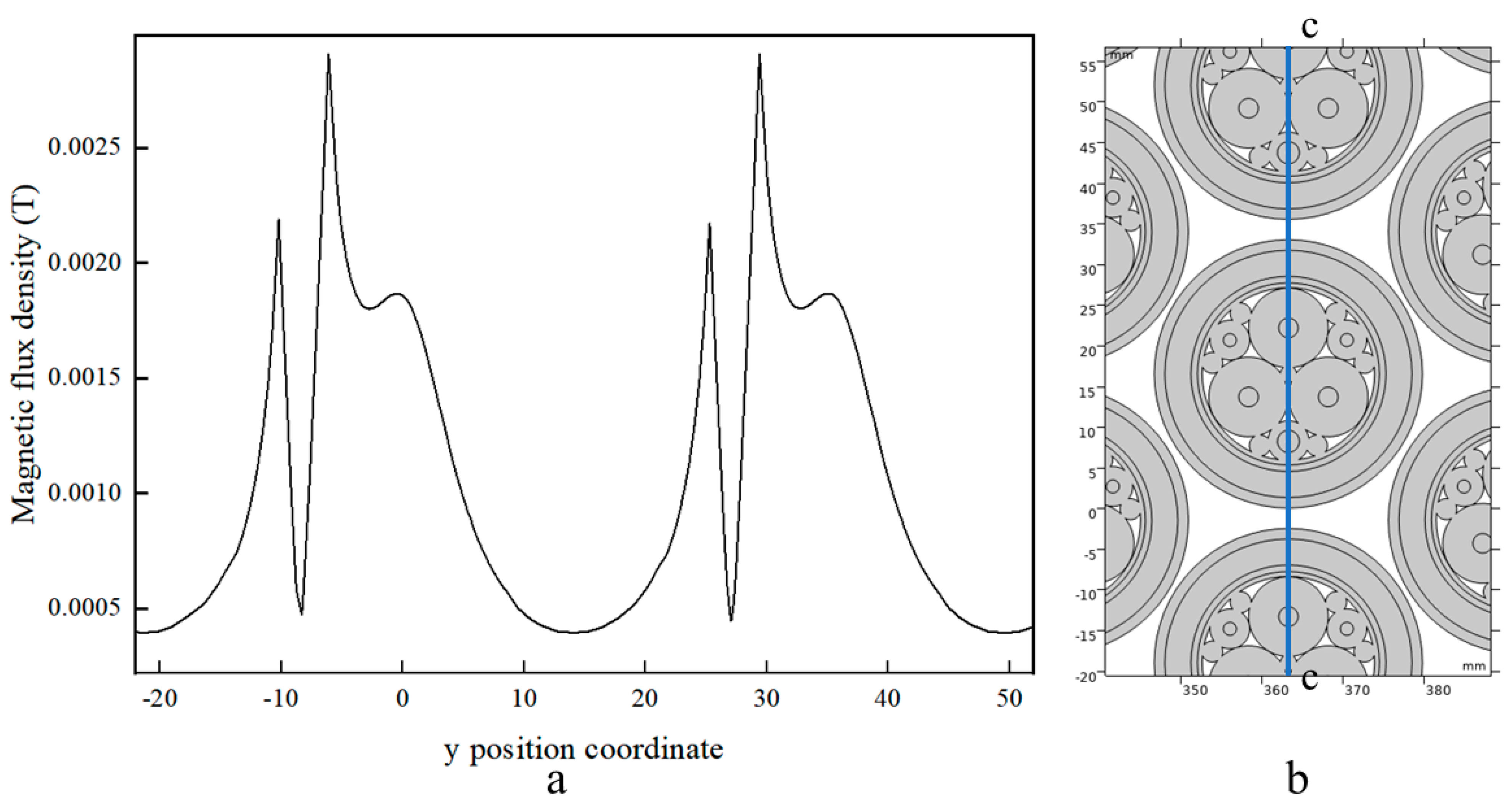
Analysed along the b–b direction, as shown in Figure 3, the tenth layer was selected. As shown in Figure 12, the MFD of a cable in the same layer shows a periodic variation with the position of the cable. As shown in Figure 13, the two cycles are locally enlarged. The periodic exhibits three peaks and two troughs. The initial peak occurs before the conductor in the cable, while the first valley is located at the centre of the conductor. After the conductor in the cable, the MFD gradually decreases to appear as a second valley. The MFD rises weakly to a third peak at the position of the centre connecting line of the two adjacent cables. It can also be seen that the centre of the cable has the lowest magnetic flux density. Therefore, arranging the signal cable here can avoid the influence of the magnetic field on it to the greatest extent.
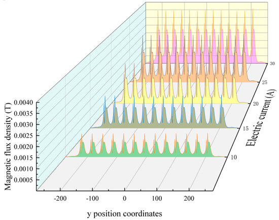
Figure 12.
MFD in the vertical axis at different currents.
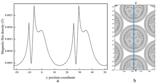
Figure 13.
Local magnification of the MFD over two cycles: (a) magnetic flux density at the c-c position; (b) Schematic diagram of c-c position coordinates.
This section shows that the maximum MFD of the system is proportional to the current and independent of the number of winding layers. Additionally, the MFD at each position exhibits periodic variation, which has to do with the conductor’s location within the cable and the separation between the cables. The period of MFD refers to the distance between the two cable layers in the radial direction from the winch centre to the outside. The MFD of the middle layer is slightly lower than that of the outer layer. In the direction of the cables on the same layer, the MFD period is the distance between the adjacent cables. Thus, the MFD in the system can be efficiently adjusted by arranging the position of the conductors and the spacing between the cables reasonably. Arranging the signal line in the centre of the cable avoids the influence of magnetic fields to the greatest extent possible.
4.2. Effect of Current on Temperature
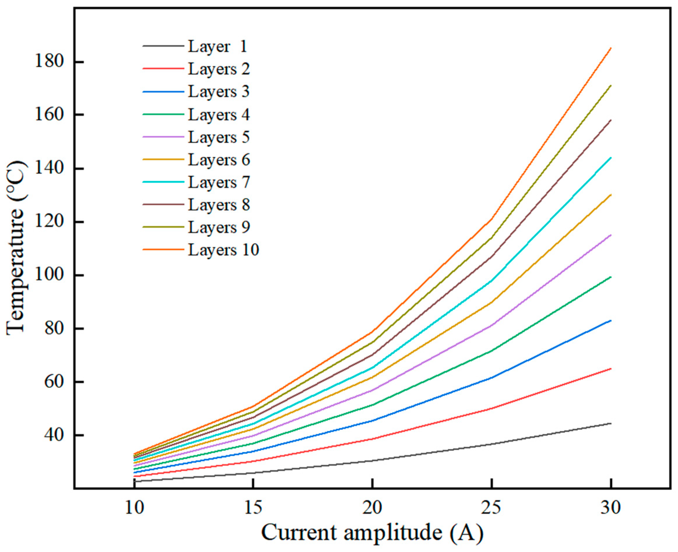
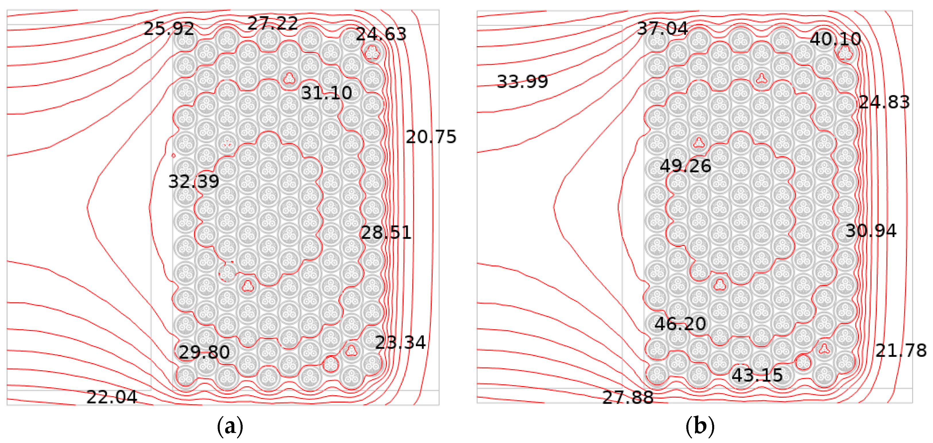
This section investigates the effect of different amplitude currents (10 A, 15 A, 20 A, 25 A, 30 A) on the temperature field in an optical cable winch system. The maximum temperature of the system significantly increases with the increase in the current and the number of winding layers, as shown in Figure 14. At the same time, the maximum temperature change in the system is analysed in the case of 1, 4 and 7 layers of winding, as shown in Table 6. At the same current, the magnitude of the temperature rise decreases as the number of winding layers increases. With the increase in the current under the same number of layers of winding, the temperature increases dramatically. Therefore, the following section will examine the impact of the number of winding layers on temperature. The temperature contours of the 10 A current, 10-layer winding system are shown in Figure 15a. The temperature distribution has a clear positional relationship, showing an inner high and outer low circular distribution, and the temperature variation of the middle layer cable is relatively small compared with that of the outside. The temperature distribution of the system was also compared for the 15 A current case. As shown in Figure 15b, the isotherm distribution is basically unchanged, but the temperature gap increases. This indicates that the current does not affect the internal temperature distribution pattern, but only the temperature amplitude and the internal and external temperature difference. Therefore, this section will continue to delve into the relationship between current magnitude and temperature at different locations in the system.
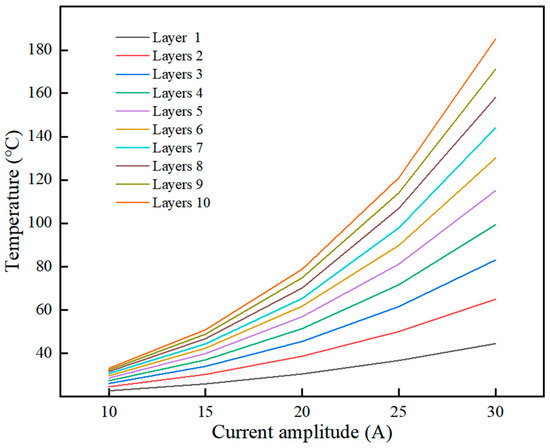
Figure 14.
Maximum temperature at different currents for layers 1–10.
Table 6.
Maximum temperature and growth rate of the system at different currents with different numbers of winding layers.
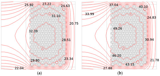
Figure 15.
Lines of equal temperature of 10-layer windings at different currents: (a) 10 A; (b) 15 A.
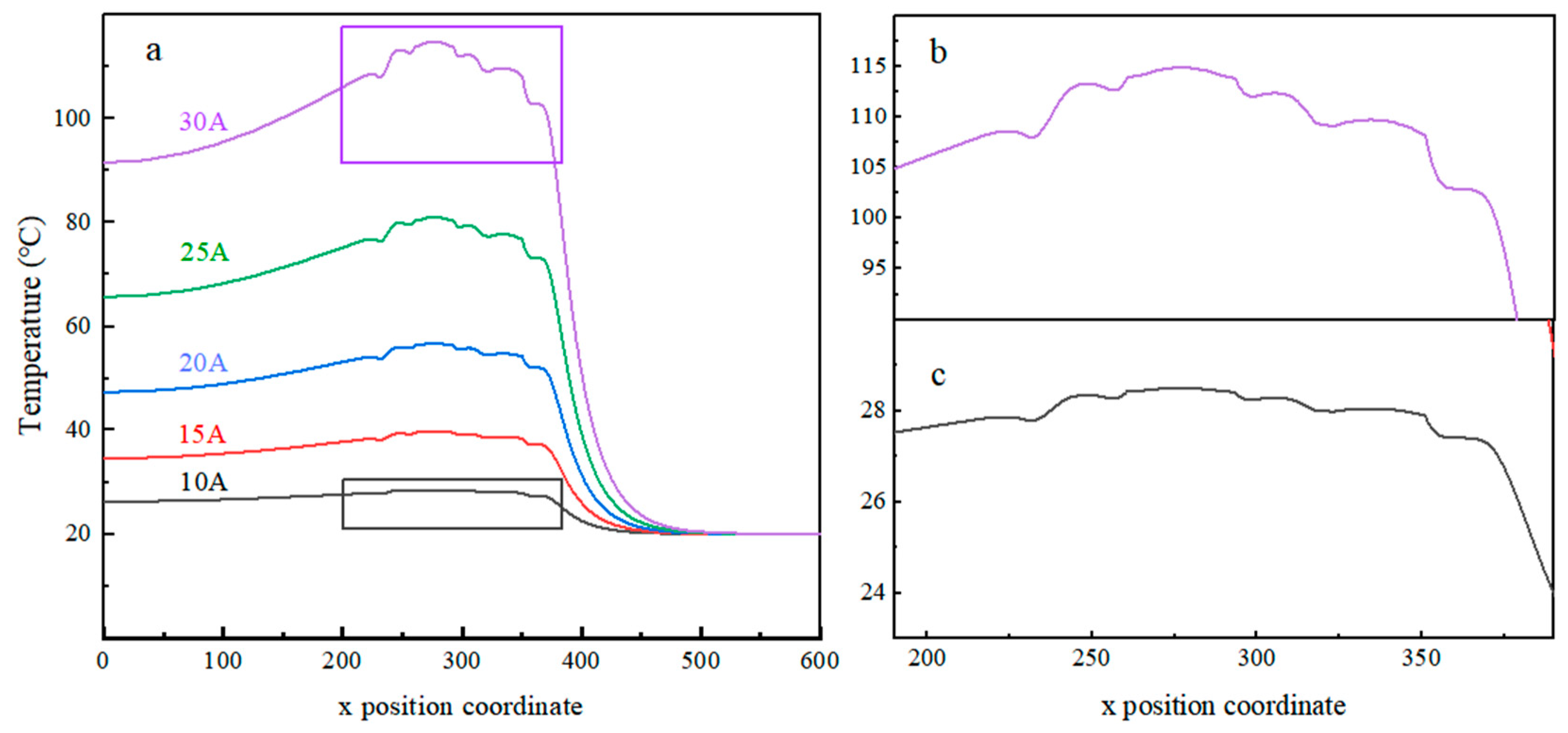
The analysis of the selected 10-layer winding case is shown in Figure 16a. The system temperature from the centre of the winch along the radial to the external temperature gradually increases until the temperature of the cable’s first layer rises dramatically. The temperature of each outward layer of cable is a leap, but the magnitude of the leap is gradually reduced to reach the highest value after the beginning of a gradual decline. To achieve greater accuracy in observing this phenomenon, the temperature rise curves of the system at 10 A and 30 A currents in Figure 16a have been locally scaled up to Figure 16b,c. After the fourth layer of cables, the temperature gradually decreases. The rate of decrease then increases until the temperature drops sharply after the tenth layer. When the quantity of winding layers remains constant but the currents are different, the temperature rise of the system follows a consistent pattern. However, as the current increases, the temperature rises and falls become more pronounced. The temperature variation in the five layers of winding is compared as shown in Figure 17, which also shows the pattern of temperature increase and then decrease, but the peak value is shifted forward, and the temperature of the second layer of the cable is the highest.
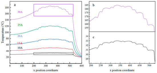
Figure 16.
The axial temperature and partial enlargement of 10-layer windings under different currents: (a) general picture; (b) the local magnified plot under the condition of 30 A current; (c) the local magnified plot under the condition of 10 A current.
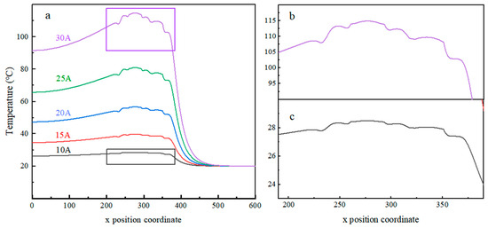
Figure 17.
The axial temperature and partial enlargement of five-layer windings under different currents: (a) general picture; (b) the local magnified plot under the condition of 30 A current; (c) the local magnified plot under the condition of 10 A current.
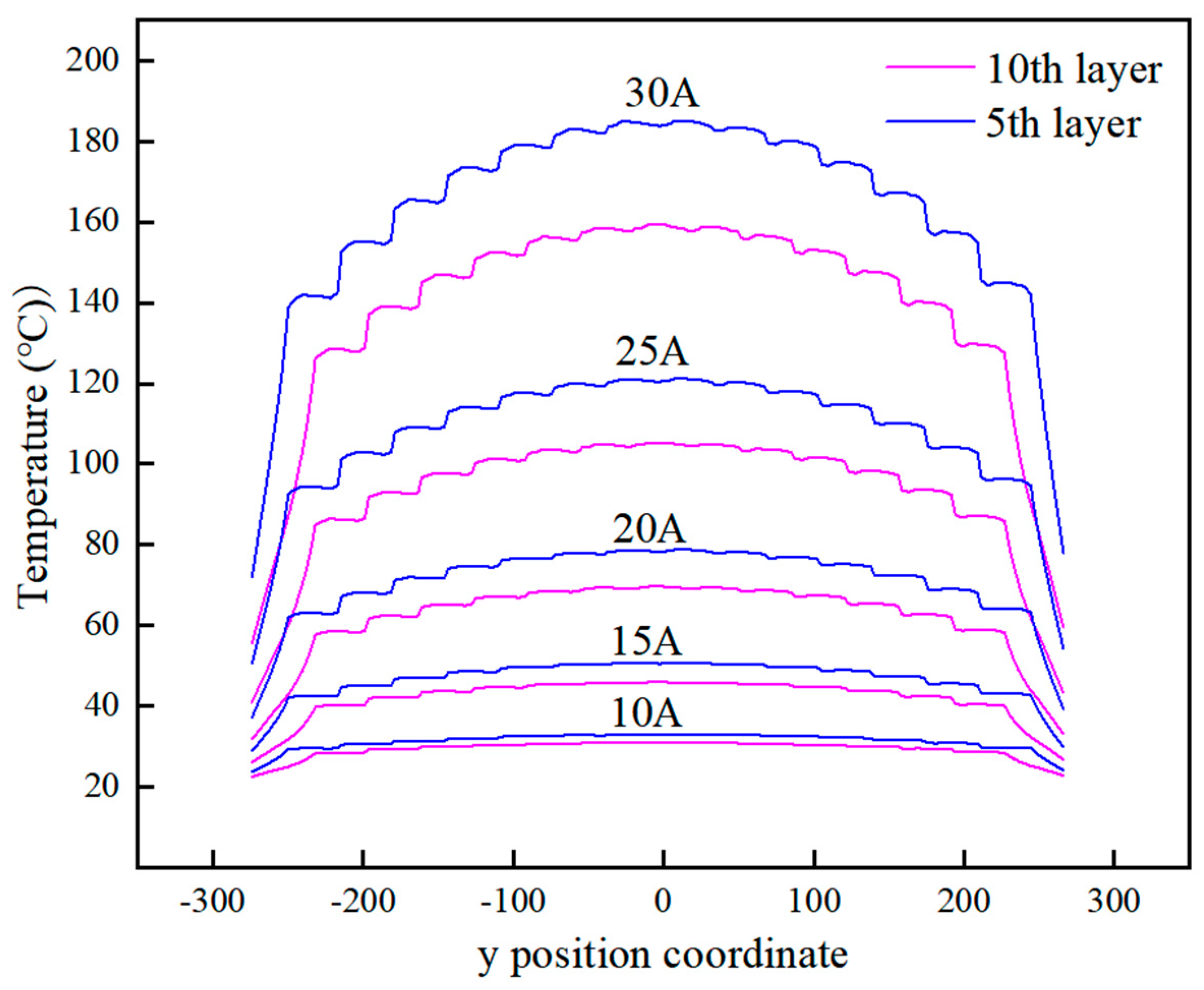
The temperature profiles of the fifth and tenth layers for 10 layers of winding and different currents are shown in Figure 18. From the margins to the centre, the cable layer’s temperature progressively rises. This increase occurs with each inward turn of the cable, and the rate of increase gradually decreases until the temperature gradually decreases after passing through the middle cable. The distribution of temperatures exhibits standard symmetry, with the axis of symmetry at the centre of this layer of cables. In the case of the same number of winding layers and different currents, the system temperature rise behaves in the same way as from the centre of the winch along the radial direction to the external position. Comparing the fifth and tenth layers, the maximum temperature difference increases with the increase in current.

Figure 18.
Temperature of the 5th and 10th layers under 10-layer winding conditions.
This section shows that the temperature distribution of the NAOCWS is related to both the current magnitude and the number of winding layers. The current has a large effect on the temperature of the system, with the temperature rising dramatically as the current rises. Along the radial direction of the winch, from the centre to the outside, the disparity in temperature between the outer and interior layers increases with the current and the number of layers. The cable layer’s temperature distribution is symmetrical. The temperature difference between the middle and edge cables increases with the current and the number of layers. Therefore, in practical applications, it is advisable to avoid the simultaneous use of high currents and multi-layer winding.
4.3. Effect of Winding Layers on System Temperature and MACCA
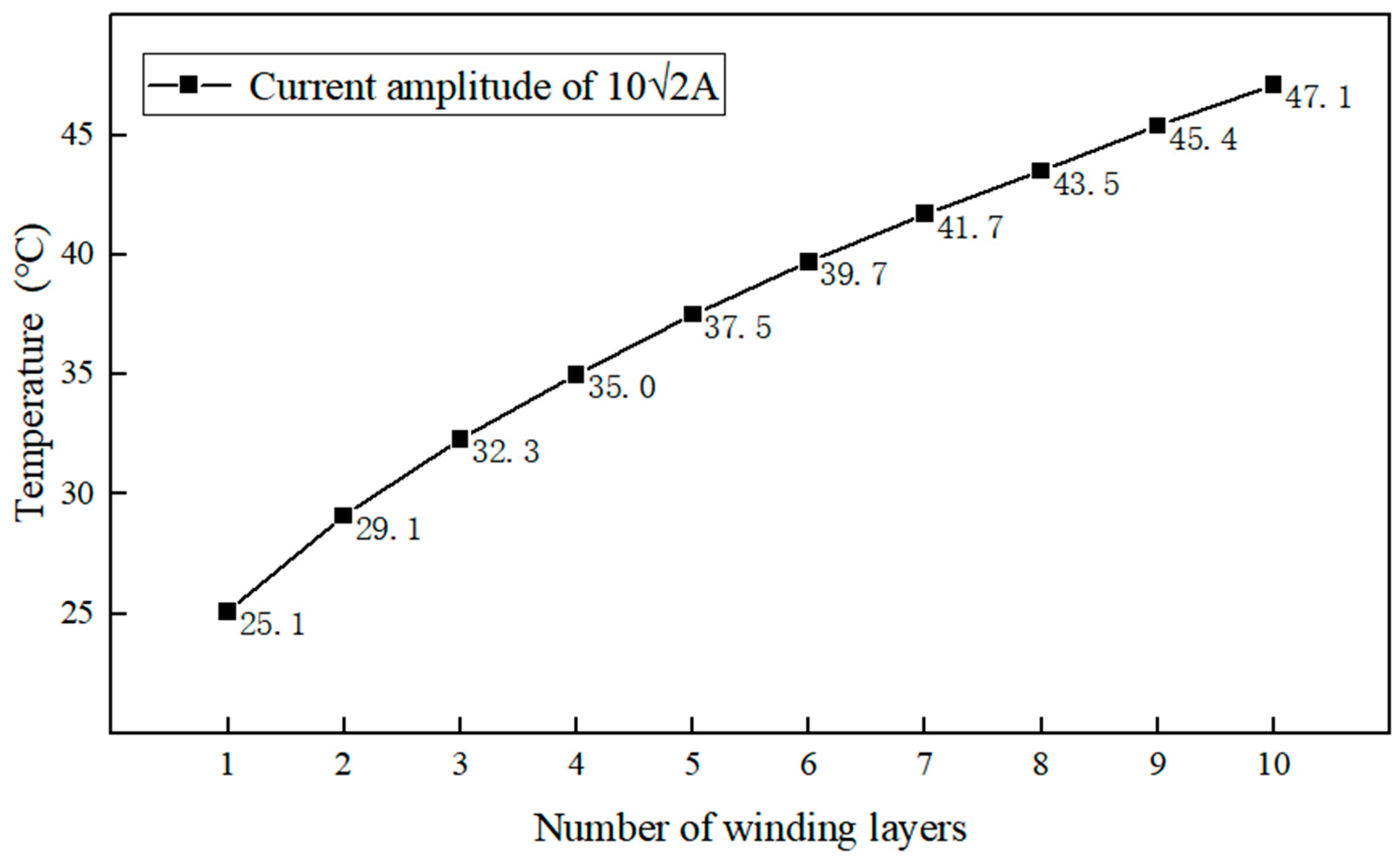
This section describes a numerical simulation of the power demand of the NAOC. The three conductor cores of the NAOC are subjected to an AC of 6.6 kV and 10 A, i.e., a 10√2 A amplitude current, consistent with the design-rated power demand.
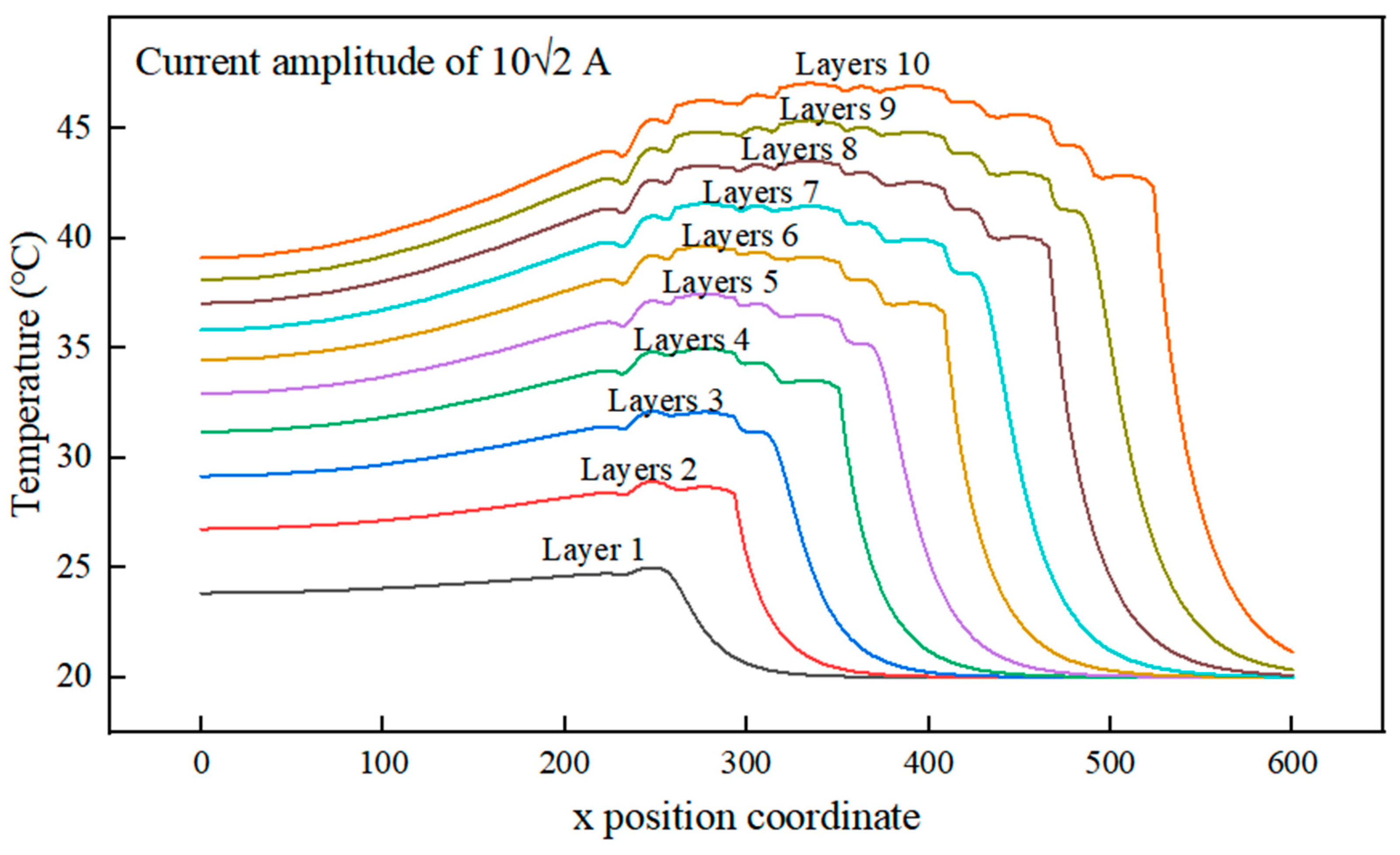
Under the same current conditions, the maximum temperature of the NAOCWS rises as the number of layers increases, as shown in Figure 19. As shown in Figure 20, by analysing the temperature change along the radial direction of the winch to the outside under different layers of winding, with an increase in the number of layers of winding, the temperature difference at each position also increases gradually, and the same nature with the highest temperature is presented. At the same time, it is found that the highest temperature is located in the number of layers, as shown in Table 7, combined with the conclusion of Section 4.2 that the current only affects the size of the temperature at each location within the system and does not affect the distribution of the temperature in the system; therefore, under the conditions of the number of winding layers, the location of the highest temperature of the system can be identified.
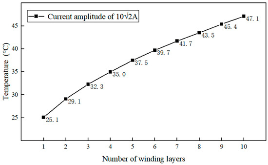
Figure 19.
Maximum temperature with different numbers of winding layers.
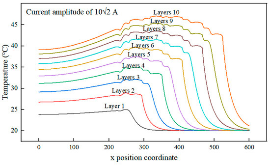
Figure 20.
Horizontal axis temperature with different numbers of winding layers.
Table 7.
Layers with the highest temperature at different numbers of winding layers.
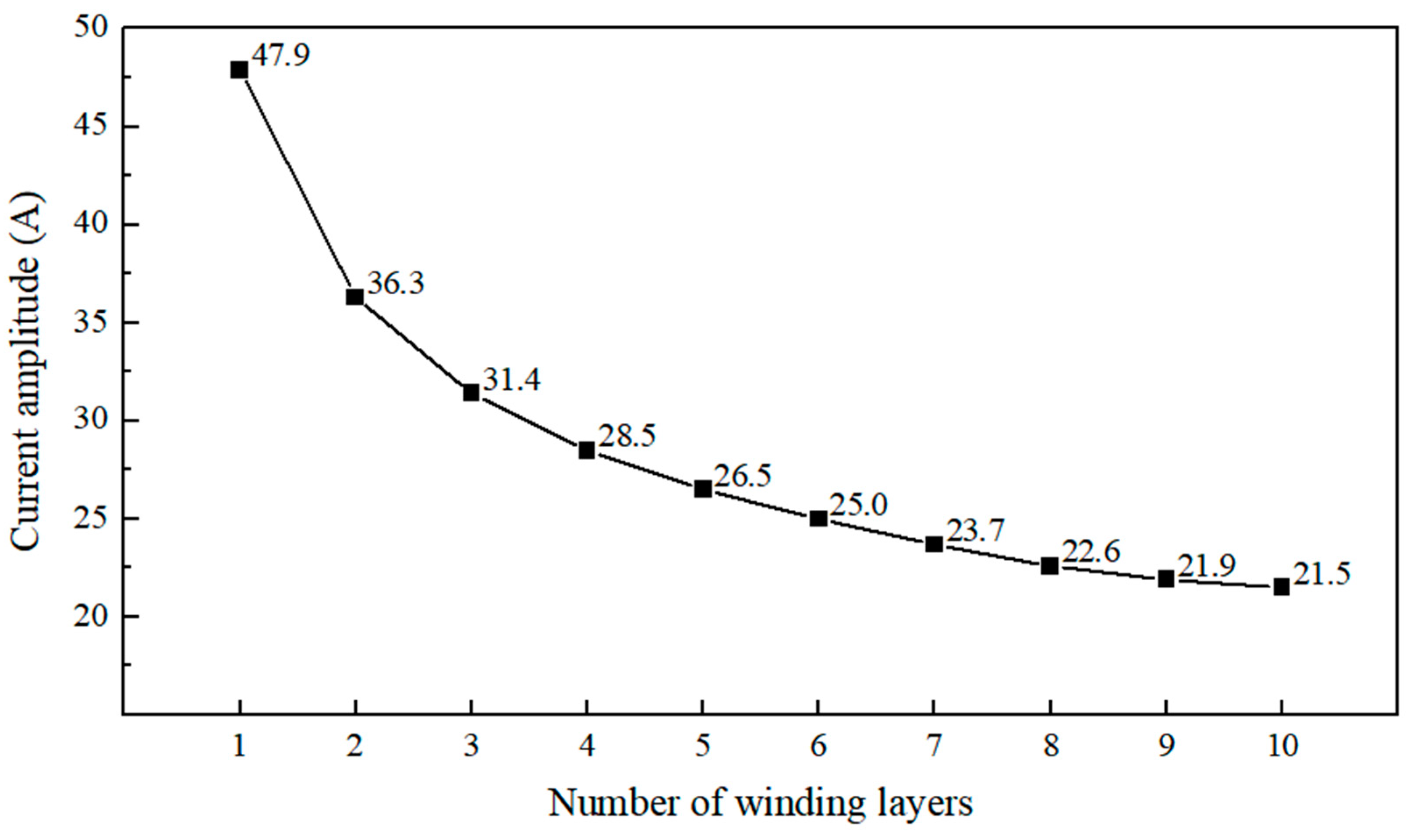
This paper uses the method described in Section 2.3 to calculate the MACCA of 1–10 layers, as shown in Figure 21. With an increase in the number of winding layers, the MACCA decreases gradually, and the decrease decreases gradually. This value provides a basis for the safe, long-term and stable operation of the system.
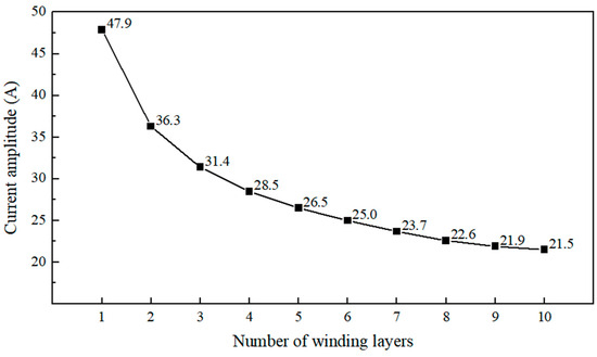
Figure 21.
MACCA at different numbers of winding layers.
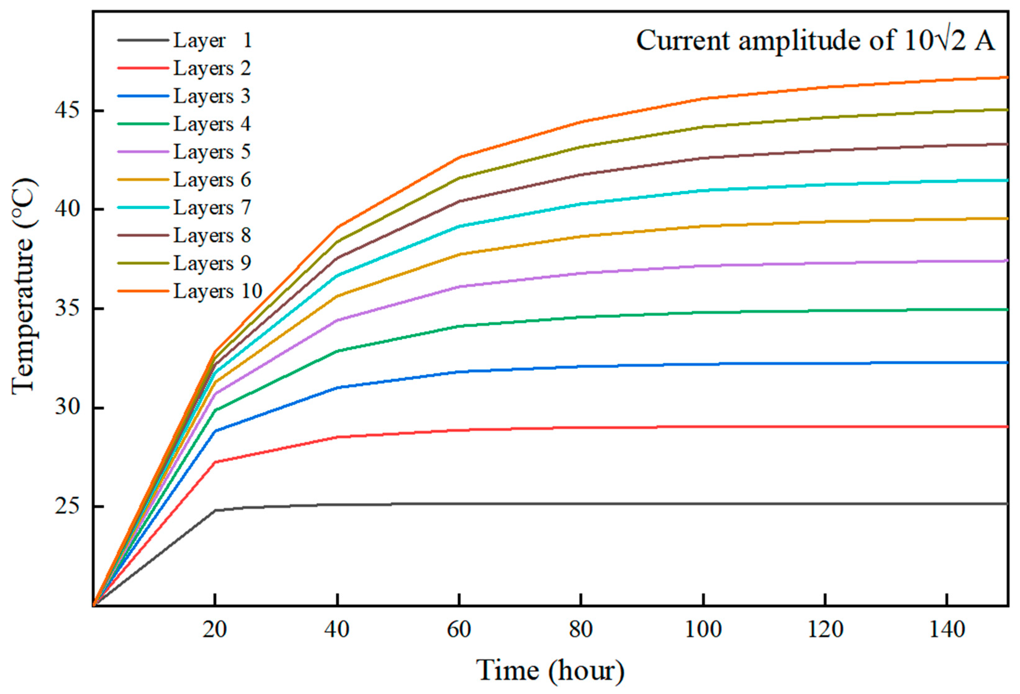
The temperature increase in the system is related not only to the number of winding layers and the current but also to the working time. As shown in Figure 22, as the number of layers increases, the time required for the system to reach a steady state increases. This phenomenon shows that increasing the number of layers leads to an increase in the system temperature, but at the same time, the time to reach a steady state is extended, so the system can be overloaded for a short period of time. This method can also be used to evaluate the safe working time at different air flow rates, currents and number of winding layers.
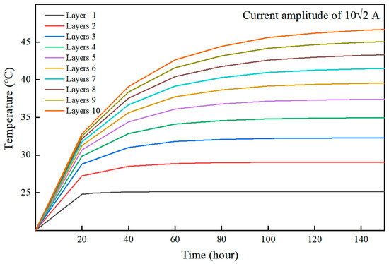
Figure 22.
Maximum system temperature versus time at different numbers of winding layers.
5. Conclusions
This paper investigates the MFD and temperature distribution of NAOCWSs in various locations using numerical calculations. The study sets different numbers of winding layers and currents following the IEC 60335-1 standard for the electromagnetic thermal characteristics of NAOCWSs. The temperature rise under different winding conditions for the rated working conditions of this system is calculated. Finally, the MACCA and the time to reach the steady state of the system are calculated for different numbers of winding layers. The main conclusions from the numerical simulations are as follows:
The maximum MFD of the system is proportional to the current and independent of the number of winding layers. The NAOC exhibits a higher internal magnetic flux density and a lower magnetic flux density on the winch. The MFD at each position exhibits periodic variation. This has to do with the conductor’s location within the cable and the separation between the cables. The period of the MFD refers to the distance between the two cable layers in a radial pattern from the winch centre outward. In the direction of the cables on the same layer, the MFD period is the distance between the adjacent cables. Thus, the MFD in the system can be efficiently altered by reasonably arranging the position of the conductors and the spacing between the cables. Arranging the signal line in the centre of the cable avoids the influence of magnetic fields to the greatest extent possible.
The system’s temperature distribution is affected by the number of winding layers, as well as the current magnitude. The current has a large effect on the temperature of the system, with a sharp increase in temperature as the current rises. Along the radial direction of the winch, from the centre to the outside, the number of layers and current magnitude both increase the temperature differential between the inner and outer layers. The current does not affect the internal temperature distribution pattern, but only the temperature amplitude and the temperature difference between the inside and outside. The cable layer’s temperature distribution is symmetrical. The temperature difference between the middle and edge cables increases with the number of layers and the current magnitude. Therefore, in practical applications, it is advisable to avoid the simultaneous use of high currents and multi-layer winding.
An increase in the number of winding layers causes the system’s temperature to rise. The greater the number of layers, the longer it takes to reach a steady state at the rated current. The layer in which the maximum temperature of the system is located at the rated current and at different numbers of winding layers is clearly defined and it does not change with the change in current and heat dissipation conditions. As the number of layers increases, the time required for the system to reach a steady state increases, so that the system can be overloaded for a short period of time.
Author Contributions
Conceptualization, W.L., H.W. and S.L.; methodology, W.L., H.W. and S.L.; software, W.L. and H.W.; validation, W.L., H.W. and S.L.; formal analysis, W.L. and H.W.; investigation, W.L., W.S. and Q.L.; resources, W.L., W.S. and Q.L.; data curation, W.L., H.W. and S.L.; writing—original draft preparation, W.L. and H.W.; writing—review and editing, W.L., H.W. and S.L.; visualization, W.L., H.W. and S.L.; supervision, W.L., W.S. and Q.L.; project administration, W.L., S.L., W.S. and Q.L.; funding acquisition, W.L., S.L. and W.S. All authors have read and agreed to the published version of the manuscript.
Funding
This research was funded by the National Key Research and Development Program of China (2023YFC2809603, 2023YFC2809601, 2022YFC2806902), the Central Guidance on Local Science and Technology Development Fund of Liaoning Province (2023JH6/100100049), Liaoning Revitalization Talents Program (XLYC2007092), 111 Project (B18009) and the Fundamental Research Funds for the Central Universities (3132023510).
Institutional Review Board Statement
Not applicable.
Informed Consent Statement
Not applicable.
Data Availability Statement
The data presented in this study are available on request from the corresponding author. The data are not publicly available due to privacy and confidentiality considerations.
Conflicts of Interest
Author Weiwei Shen was employed by the company HMN Technologies Group Co., Ltd. and author Qingtao Lv was employed by the company Nantong Liwei Machinery Co., Ltd. The remaining authors declare that the research was conducted in the absence of any commercial or financial relationships that could be construed as a potential conflict of interest.
References
- Foster, G.P. Advantages of fiber rope over wire rope. J. Ind. Text. 2002, 32, 67–75. [Google Scholar] [CrossRef]
- Liu, Z.; Soares, C.G. Numerical study of rope materials of the mooring system for gravity cages. Ocean Eng. 2024, 298, 117135. [Google Scholar] [CrossRef]
- Ye, H.; Li, W.; Lin, S.; Ge, Y.; Lv, Q. A framework for fault detection method selection of oceanographic multi-layer winch fibre rope arrangement. Measurement 2024, 226, 114168. [Google Scholar] [CrossRef]
- Wait, J.R. Electromagnetic wave propagation along a buried insulated wire. Can. J. Phys. 1972, 50, 2402–2409. [Google Scholar] [CrossRef]
- Wait, J.R. Excitation of currents on a buried insulated cable. J. Appl. Phys. 1978, 49, 876–880. [Google Scholar] [CrossRef]
- Bridges, G.E. Transient plane wave coupling to bare and insulated cables buried in a lossy half-space. IEEE Trans. Electromagn. Compat. 1995, 37, 62–70. [Google Scholar] [CrossRef]
- Hutchison, Z.L.; Gill, A.B.; Sigray, P.; He, H.; King, J.W. A modelling evaluation of electromagnetic fields emitted by buried subsea power cables and encountered by marine animals: Considerations for marine renewable energy development. Renew. Energy 2021, 177, 72–81. [Google Scholar] [CrossRef]
- Expethit, A.; Sørensen, S.; Arentsen, M.; Pedersen, M.; Sørensen, D.; da Silva, F. MVAC Submarine cable, magnetic fields measurements and analysis. In Proceedings of the 2017 52nd International Universities’ Power Engineering Conference (UPEC), Heraklion, Greece, 28–31 August 2017; pp. 28–31. [Google Scholar]
- Hutchison, Z.L.; Secor, D.H.; Gill, A.B. The interaction between resource species and electromagnetic fields associated with electricity production by offshore wind farms. Oceanography 2020, 33, 96–107. [Google Scholar] [CrossRef]
- Xue, H.; Ametani, A.; Yamamoto, K. Theoretical and NEC calculations of electromagnetic fields generated from a multi-phase underground cable. IEEE Trans. Power Deliv. 2020, 36, 1270–1280. [Google Scholar] [CrossRef]
- Gill, A.B.; Huang, Y.; Spencer, J.; Gloyne-Philips, I. Electromagnetic fields emitted by high voltage alternating current offshore wind power cables and interactions with marine organisms. In Proceedings of the Electromagnetics in Current and Emerging Energy Power Systems Seminar, London, UK, 17–24 June 2012. [Google Scholar]
- Del-Pino-López, J.C.; Cruz-Romero, P.; Bravo-Rodríguez, J.C. Evaluation of the power frequency magnetic field generated by three-core armored cables through 3D finite element simulations. Electr. Power Syst. Res. 2022, 213, 108701. [Google Scholar] [CrossRef]
- IEC 60287; Electric Cables-Calculation of the Current Rating. International Electrotechnical Commission: Geneva, GE, Switzerland, 2023.
- Karahan, M.; Kalenderli, O.; Vikhrenko, V. Coupled electrical and thermal analysis of power cables using finite element method. Heat Transf. Eng. Appl. 2011, 9, 205–230. [Google Scholar]
- Xu, X.; Yuan, Q.; Sun, X.; Hu, D.; Wang, J. Simulation analysis of carrying capacity of tunnel cable in different laying ways. Int. J. Heat Mass Transf. 2019, 130, 455–459. [Google Scholar] [CrossRef]
- Demirol, Y.B.; Kalenderli, Ö. Investigation of effect of laying and bonding parameters of high-voltage underground cables on thermal and electrical performances by multiphysics FEM analysis. Electr. Power Syst. Res. 2024, 227, 109987. [Google Scholar] [CrossRef]
- Rasoulpoor, M.; Mirzaie, M.; Mirimani, S. Thermal assessment of sheathed medium voltage power cables under non-sinusoidal current and daily load cycle. Appl. Therm. Eng. 2017, 123, 353–364. [Google Scholar] [CrossRef]
- Maximov, S.; Venegas, V.; Guardado, J.; Moreno, E.; López, R. Analysis of underground cable ampacity considering non-uniform soil temperature distributions. Electr. Power Syst. Res. 2016, 132, 22–29. [Google Scholar] [CrossRef]
- Trufanova, N.; Navalikhina, E.Y.; Gataulin, T. Mathematical modeling of nonstationary processes of heat and mass transfer in a rectangular cable channel. Russ. Electr. Eng. 2015, 86, 656–660. [Google Scholar] [CrossRef]
- Bangay, J.; Coleman, M.; Batten, R. Comparison of IEEE and CIGRE methods for predicting thermal behaviour of powerlines and their relevance to distribution networks. In Proceedings of the 2015 IEEE Eindhoven PowerTech, Eindhoven, The Netherlands, 29 June–2 July 2015; pp. 1–5. [Google Scholar]
- Chen, W.; Zhou, M.; Yan, X.; Li, Z.; Lin, X. Study on electromagnetic-fluid-temperature multiphysics field coupling model for drum of mine cable winding truck. CES Trans. Electr. Mach. Syst. 2021, 5, 133–142. [Google Scholar] [CrossRef]
- Ravichandran, R.; Umapathy, A.; Babu, S.M.; Vedhachalam, N.; Venkatesan, K.; Harikrishnan, G.; Subramanium, A.; Ramadass, G.; Atmanand, M. Heat dissipation studies on sub-sea cables wound on winches. In Proceedings of the 2015 IEEE Underwater Technology (UT), Chennai, India, 23–25 February 2015; pp. 1–4. [Google Scholar]
- Ghoneim, S.S.M.; Ahmed, M.; Sabiha, N.A. Transient thermal performance of power cable ascertained using finite element analysis. Processes 2021, 9, 438. [Google Scholar] [CrossRef]
- Malinowski, M.; Kubiczek, K.; Kampik, M. A precision coaxial current shunt for current AC-DC transfer. Measurement 2021, 176, 109126. [Google Scholar] [CrossRef]
- Kubiczek, K.; Kampik, M. Fast and Numerically Stable Analytical Computations for the Power Induced in Cylindrical Multilayered Conductors Under External Magnetic Fields. IEEE Trans. Electromagn. Compat. 2022, 65, 292–299. [Google Scholar] [CrossRef]
- Hu, M. Calculation of Thermal Distribution and Ampacity for High-Voltage Power Cables by Using Multi-Physics Coupled Model. Master’s Thesis, South China University of Technology, Guangzhou, China, 2015. [Google Scholar]
- Dubitsky, S.; Greshnyakov, G.; Korovkin, N. Comparison of finite element analysis to IEC-60287 for predicting underground cable ampacity. In Proceedings of the 2016 IEEE International Energy Conference (ENERGYCON), Leuven, Belgium, 4–8 April 2016; pp. 1–6. [Google Scholar]
- Stebel, M.; Kubiczek, K.; Rodriguez, G.R.; Palacz, M.; Garelli, L.; Melka, B.; Haida, M.; Bodys, J.; Nowak, A.J.; Lasek, P. Thermal analysis of 8.5 MVA disk-type power transformer cooled by biodegradable ester oil working in ONAN mode by using advanced EMAG–CFD–CFD coupling. Int. J. Electr. Power Energy Syst. 2022, 136, 107737. [Google Scholar] [CrossRef]
- Zhao, Z. Research on Fast Calculation Method for Transient Temperature Rise of Cable Core of Power Cables in Duck. Master’s Thesis, Hebei University of Science and Technology, Shijiazhuang, China, 2022. [Google Scholar]
- Che, C.; Yan, B.; Fu, C.; Li, G.; Qin, C.; Liu, L. Improvement of cable current carrying capacity using COMSOL software. Energy Rep. 2022, 8, 931–942. [Google Scholar] [CrossRef]
- Takahashi, N.; Nakata, T.; Fujii, Y.; Muramatsu, K.; Kitagawa, M.; Takehara, J. 3-D finite element analysis of coupling current in multifilamentary AC superconducting cable. IEEE Trans. Magn. 1991, 27, 4061–4064. [Google Scholar] [CrossRef]
- Cengel, Y.A.; Ghajar, A.J. Introduction and basic concepts. In Heat and Mass Transfer Fundamental and Applications; McGraw-Hill Education: New York, NY, USA, 2015; pp. 7–10. [Google Scholar]
- Gao, M.; Cui, W.-B.; Zhang, L.-S.; Zhang, B.-H.; Lou, Q. Comparative investigation of numerical simulation and experimental study of electroconvection layer in natural convection heat transfer enhanced by an electric field. Int. Commun. Heat Mass Transf. 2024, 153, 107344. [Google Scholar] [CrossRef]
- Fouda, B.M.T.; Han, D.; Zhang, W.; An, B. Research on key technology to determine the exact maximum allowable current-carrying ampacity for submarine cables. Opt. Laser Technol. 2024, 175, 110705. [Google Scholar] [CrossRef]
- IEC 60335-1; Household and Similar Electrical Appliances-Safety. International Electrotechnical Commission: Geneva, GE, Switzerland, 2020.

Disclaimer/Publisher’s Note: The statements, opinions and data contained in all publications are solely those of the individual author(s) and contributor(s) and not of MDPI and/or the editor(s). MDPI and/or the editor(s) disclaim responsibility for any injury to people or property resulting from any ideas, methods, instructions or products referred to in the content. |
© 2024 by the authors. Licensee MDPI, Basel, Switzerland. This article is an open access article distributed under the terms and conditions of the Creative Commons Attribution (CC BY) license (https://creativecommons.org/licenses/by/4.0/).