Graph Search-Based Path Planning for Automatic Ship Berthing

Abstract

Ship berthing is one of the most challenging operations for crews, involving optimal trajectory generation and intricate harbor maneuvering at low speed. In this paper, we present a practical path-planning method that generates smooth trajectories for an underactuated surface vehicle (USV) traveling in a confined harbor environment. Our approach introduces a Generalized Voronoi Diagram (GVD)-based path planner to handle the unberthing phase. The hybrid A* search-based path finding method is used for the transportation phase. A simple planner based on a Bézier curve is proposed for the berthing phase. To track the target path, an adaptive pure pursuit method and proportional-derivative (PD) controller is used. The performance of the given method is tested numerically and experimentally on a catamaran with a pair of non-steerable thrusters. The results demonstrate that the proposed algorithm can achieve a successful berthing operation through static obstacle handling and smooth trajectory generation.

1. Introduction

Bringing about an automatic berthing system for USVs is a complicated task. Such an operation involves moving from open waters or a harbor area toward the berthing position, which requires advanced maneuvering skills. Especially when the ship hits the quay, high-precision movements are required for motion control. Therefore, it is necessary to conduct research into the automatic berthing operation.

The full-scale experiment on the automatic berthing operation of a fully-actuated surface vehicle was demonstrated in the 1990s [1]. Since then, various studies have been performed on the simple berthing operation without surrounding obstacles. The motion control of the berthing operation is highly nonlinear, as various types of maneuvers are required, including reversal, turning, stopping and accelerating motion. Due to the nonlinearity of the ship’s motion, many researchers solved the berthing problem using the optimal control, which was modeled as a minimum-time optimization problem. The discrete augmented Lagrangian approach [2] was used to generate the optimal trajectory while considering the actuator capacity and nonlinearity of the ship model. A covariance matrix adaptation evolution strategy (CMA-ES) [3] solver was used to give the berthing solutions. A multiple shooting algorithm [4] has been introduced to give the sub-optimal solution for the minimum-time optimization problem. An artificial neutral network (ANN) [5,6,7,8] has been proposed to learn how to navigate from the starting position to the berthing quay. The ANN was trained using the simulated data under different wind conditions. The effectiveness of the ANN-based path planner has been verified in the automatic berthing simulation under wind disturbance. A hybrid method [9] has been proposed to predict the ship motion, based on the ANN and dynamic model. The trained data include the relative wind speed and direction, measured position, altitude and velocity, etc. However, it is essential to consider the harbor geometry and surrounding obstacles in the path-planning method for the automatic berthing operation.

To consider the harbor layout and surrounding obstacles, the optimization-based path planners are often preferable, as the vehicle constraints, path smoothness and dynamic environments can be explicitly formulated as an optimization problem. The berthing problem was formulated as a nonlinear programming one [10], where the spatial constraints were enforced through a convex approximation of the collision-free reachable space. The simulation demonstrated that their proposed method could generate a collision-free path toward the target pose. The multi-objective optimization [11] with the trade-off between energy consumption, berthing accuracy and collision avoidance was presented for the path planning of the berthing and unberthing operation. The effects of wind disturbance and user-specified waypoints were also considered in the optimization problem. To generate more efficient trajectories, the pseudo-Huber cost was introduced in the cost function of online optimization [12]. Their method utilizes the real-time mapping of the harbor and obstacles using LIDAR and ultrasonic sensors. For these optimization-based approaches, the optimization is non-convex and time-consuming; this means the feasible and efficient trajectory generation cannot be guaranteed [13].

To develop fast and online algorithms for the berthing trajectory, the graph search methods [14], including Dijkstra, the A* and D* algorithm, etc., can be useful in finding a feasible path from the starting position to the berthing pose. For the search-based planner, the state space of a vehicle is represented as a discrete grid space, where the smoothness of the best path cannot be guaranteed. The hybrid A* algorithm [15] was proposed to generate a drivable path for a self-driving car in the unstructured environment. By replacing the discrete state spaces with the precomputed motion primitives, the hybrid A* method can take into account the physical limits of a vehicle. However, the best paths produced by hybrid A* are not smooth and often sub-optimal. Further improvement of the resulting A* path is required. The path smoothing method based on a Voronoi potential field [16] was used to improve the quality of the resulting path. In [17], the authors utilized the hybrid A* path as a warm start to the nonlinear optimization, which produced the smooth and energy-optimized trajectory for the berthing operation.

A practical path-planning algorithm for the berthing operation must generate a smooth, feasible and obstacle-free path in real-time, while maintaining the accuracy required for the berthing control. In this paper, we present a two-stage path planner for the berthing operation of a small USV. At the first stage, we extend the hybrid-state A* search with analytic expansions based on the Dubins curve [18]. It considers the kinematic constraints of the USV by constructing motion primitives. The improvement of the resulting A* path is achieved by a path smoother. If the hybrid A* search fails to find a solution, it will produce a temporary path based on the Generalized Voronoi Diagram (GVD) of the surrounding obstacles. During the second stage, it is assumed that there is no dynamic obstacle between the final berthing state and the goal state of the hybrid A* search. A cubic Bézier curve is used to link these two states, which can guide the vehicle into the final berthing pose with sufficient precision. The pure pursuit method and PD controller are implemented to track the target path, which is the concatenation of two stages (see Figure 1). In the experiments on a small USV equipped with a pair of non-steerable thrusters, the proposed method can generate a collision-free and smooth path and achieves successful berthing.

2. Theoretical Background

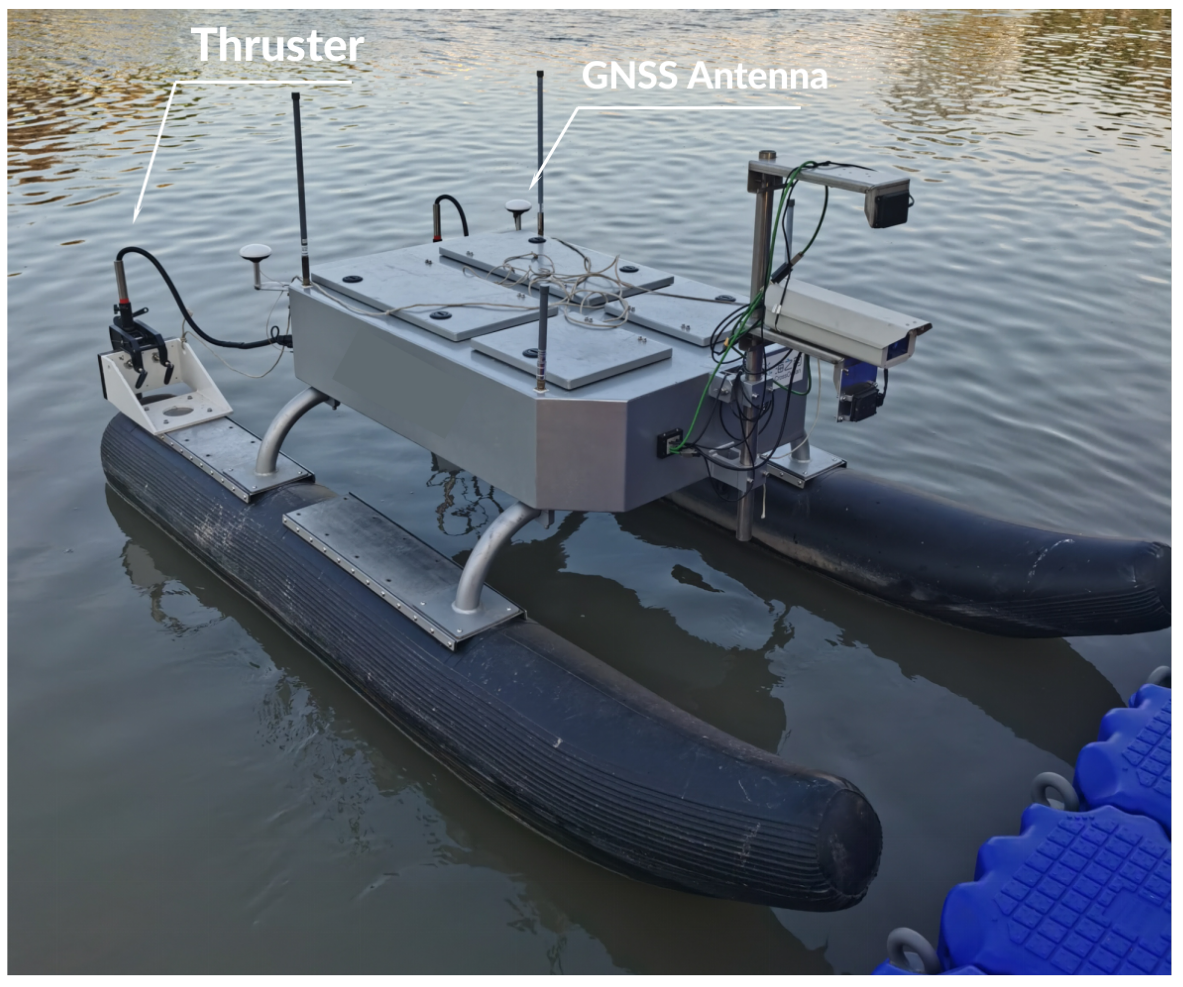
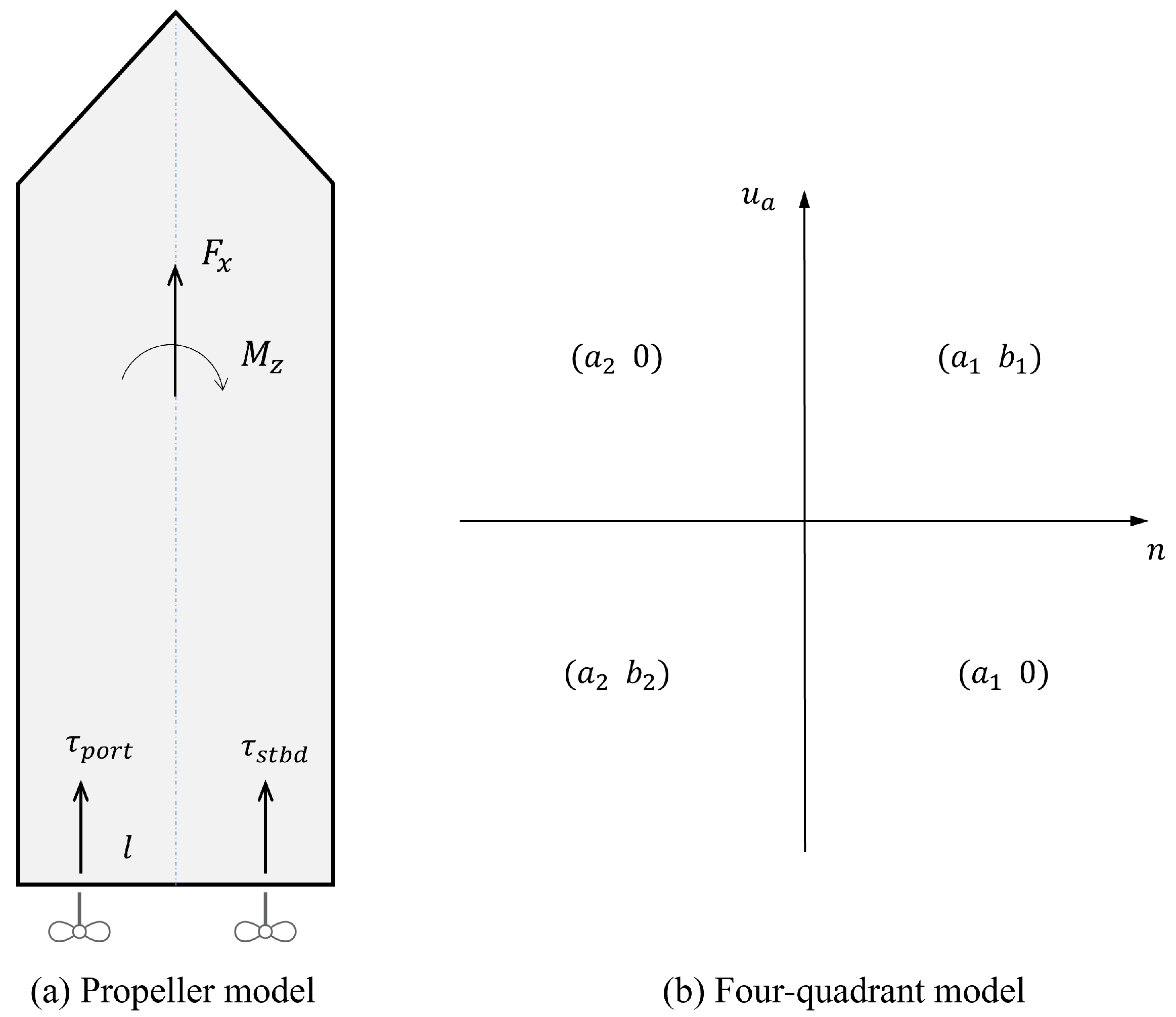
2.1. Modelling and Identification

The experimental USV (see Figure 2) is equipped with a pair of propellers, whose parameters are listed in

Table 1. Vehicle specifications.

Items	Unit	Value
Length	$\mathrm{m}$	3.1
Width	$\mathrm{m}$	1.8
Weight	$\mathrm{kg}$	244.0
CoG	$\mathrm{m}$	0.68

. We develop and implement a 3-Degree of Freedom (DoF) equation of motion for USV.

$$\dot{\mathit{\eta }}=\mathit{T}\left(\mathit{\eta }\right)·\mathbf{v},\mathit{T}\left(\mathit{\eta }\right)=\left[\begin{array}{ccc}cos\phi & -sin\phi & 0\\ sin\phi & cos\phi & 0\\ 0& 0& 1\end{array}\right]$$

(1)

$$\left({\mathit{M}}_{RB}+{\mathit{M}}_A\right)·\dot{\mathbf{v}}+\left({\mathit{C}}_{RB}\left(\mathbf{v}\right)+{\mathit{C}}_A\left(\mathbf{v}\right)+\mathit{D}\left(\mathbf{v}\right)\right)·\mathbf{v}={\mathit{\tau }}_{\mathbf{c}}$$

(2)

Here, vector $\mathit{\eta }={[N,E,\phi ]}^{\mathrm{T}}$ contains position $(N,E)$ in the north and east coordinates and is heading $\phi$ from true north. $\mathbf{v}={[u,v,r]}^{\mathrm{T}}$ denotes velocity vector in the body-fixed coordinate; $u,v,r$ are surge, sway velocity and rate of turning, respectively. $\mathit{T}\left(\mathit{\eta }\right)$ is the coordinate transformation matrix. According to the literature [19],

$${\mathit{M}}_{RB}=\left[\begin{array}{ccc}m& 0& 0\\ 0& m& m{x}_g\\ 0& m{x}_g& I_z\end{array}\right], {\mathit{M}}_A=\left[\begin{array}{ccc}-X_{\dot{u}}& 0& 0\\ 0& -Y_{\dot{v}}& -Y_{\dot{r}}\\ 0& -N_{\dot{v}}& -N_{\dot{r}}\end{array}\right]$$

(3)

where m denotes the mass, $x_g$ center of gravity (CoG) and $I_z$ denotes moment of inertia about z-axis. The Coriolis ${\mathit{C}}_{RB}\left(\mathbf{v}\right)$, centrifugal ${\mathit{C}}_A\left(\mathbf{v}\right)$ and damping matrix $\mathit{D}\left(\mathbf{v}\right)$ are given by

$${\mathit{C}}_{RB}\left(\mathbf{v}\right)+{\mathit{C}}_A\left(\mathbf{v}\right)=\left[\begin{array}{ccc}0& -mr& -m{x}_{g}r+Y_{\dot{v}}v+\gamma \\ mr& 0& -X_{\dot{u}}u\\ m{x}_{g}r-Y_{\dot{v}}v-\gamma r& X_{\dot{u}}u& 0\end{array}\right], \gamma =\frac{Y_{\dot{r}}+N_{\dot{v}}}{2}$$

(4)

$$\mathit{D}\left(\mathbf{v}\right)=-\left[\begin{array}{ccc}{X}_u+X_{\left|u\right|u}\left|u\right|& 0& 0\\ 0& Y_v+Y_{\left|v\right|v}\left|v\right|& 0\\ 0& 0& N_r+N_{\left|r\right|r}\left|r\right|\end{array}\right]$$

(5)

The linear drag and quadratic drag coefficient are considered in damping matrix. Figure 3a shows the propellers on PORT and STBD side. By calculating the thrust ${\tau }_{\mathrm{port}}$ and ${\tau }_{\mathrm{stbd}}$ of two propellers, the control input ${\mathit{\tau }}_{\mathrm{c}}$ is given by

$${\mathit{\tau }}_{\mathrm{c}}=\left[{\tau }_{\mathrm{port}}+{\tau }_{\mathrm{stbd}}, 0, \left({\tau }_{\mathrm{port}}-{\tau }_{\mathrm{stbd}}\right)l\right]$$

(6)

For each propeller, the thrust force is given by

$${\tau }_e=c_1\rho d^4\left|n\right|n-c_2\rho d^3{u}_a\left|n\right|$$

(7)

where $\rho ,d,n$ denote the water density, propeller diameter and the rotational speed, respectively. The inflow velocity $u_a$ of each propeller is calculated independently:

$$u_{a-port}=u+lr{u}_{a-stbd}=u-lr$$

(8)

The four-quadrant model [20] is used for coefficients $(c_1,c_2)$. As shown in Figure 3b, $c_1=a_2,c_2=0$ if $n<0,u_a\ge 0$, and so on. With $\rho =1000\mathrm{kg}/{\mathrm{m}}^3,d=0.24\mathrm{m},l=0.68\mathrm{m}$, the identification of the modelling parameters (see

Table 2. The modeling parameters of USV.

Items	Unit	Value
$I_z$	$\mathrm{kg}$	192.0
$Y_{\dot{v}}$	$\mathrm{kg}$	−72.1
$Y_{\dot{r}}$	$\mathrm{kgm}$	−179.2
$N_{\dot{v}}$	$\mathrm{kgm}$	−132.8
$N_{\dot{r}}$	${\mathrm{kgm}}^2$	−828.8
$X_u$	$\mathrm{Ns}/\mathrm{m}$	−8.6
$Y_v$	$\mathrm{Ns}/\mathrm{m}$	−232.3
$N_r$	$\mathrm{Nms}/\mathrm{rad}$	−171.2
$X_{\left|u\right|u}$	$\mathrm{N}{\mathrm{s}}^2/{\mathrm{m}}^2$	−48.5
$Y_{\left|v\right|v}$	$\mathrm{N}{\mathrm{s}}^2/{\mathrm{m}}^2$	−81.2
$N_{\left|r\right|r}$	$\mathrm{N}$	−163.1

) was performed using the zigzag and spiral maneuver test as well as a bollard pull test. The more detailed description of such a model identification test can be found in this paper [21].

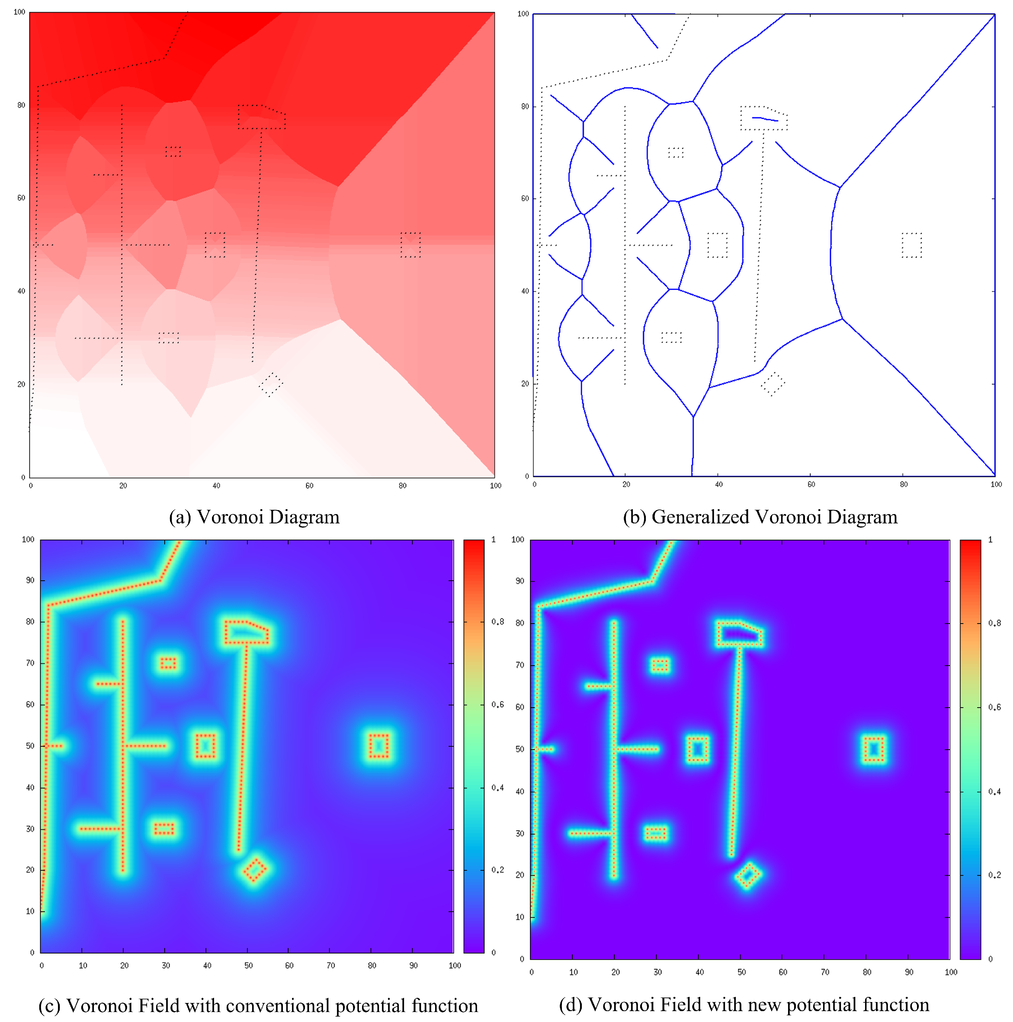
2.2. Generalized Voronoi Diagram (GVD)

If the edges of each obstacle are decomposed into many discrete points, we can generate a Voronoi diagram on a 2-dimensional plane around these points using Fortune’s algorithm [22]. When the eliminations on those Voronoi edges intersect one of the obstacles, the remaining edges form a good approximation of the Generalized Voronoi Diagram (GVD) [23]. The GVD provides the safest path around the environment, such as obstacles or areas that the vehicle cannot traverse. Figure 4a,b shows an example of the Voronoi diagram and GVD.

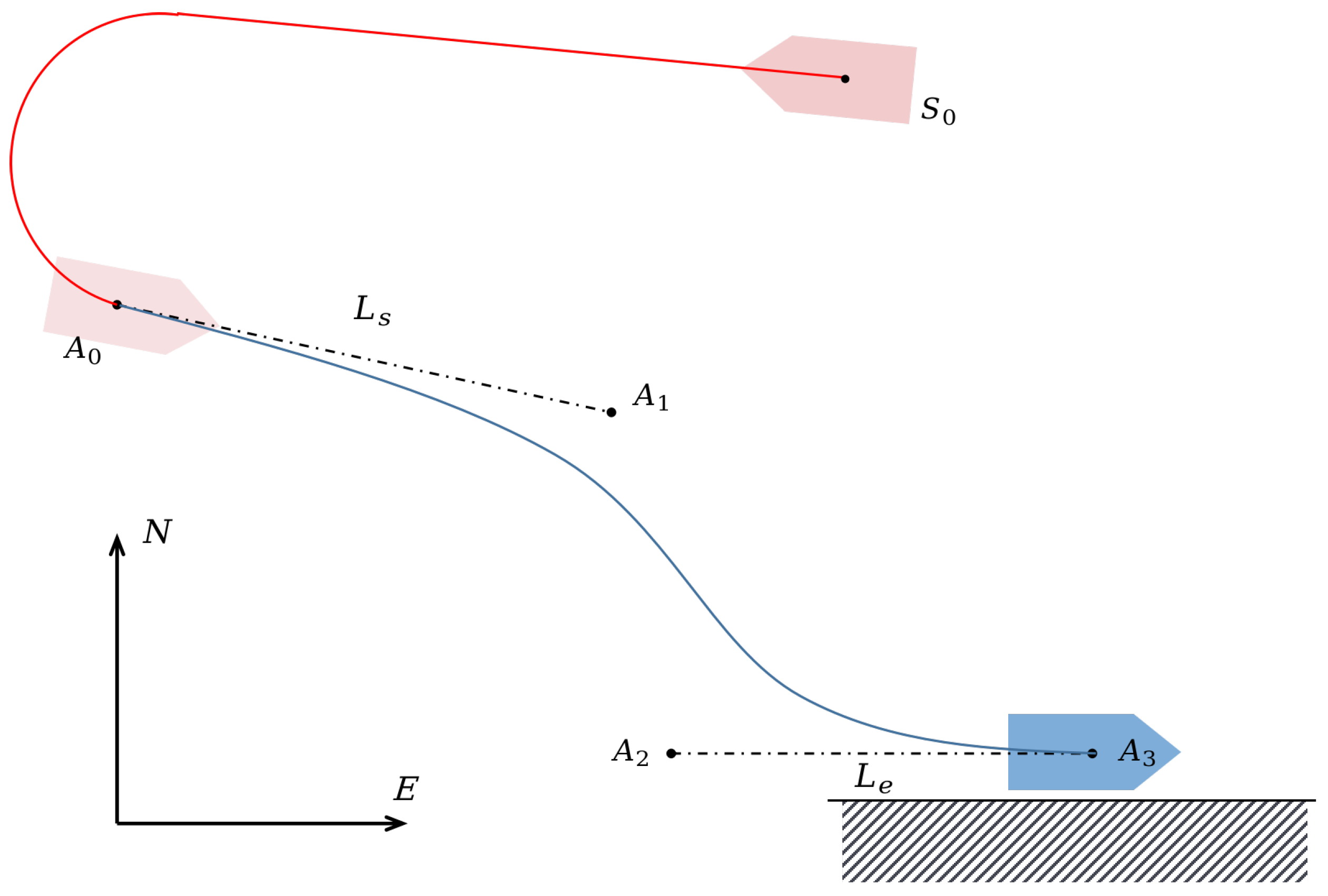
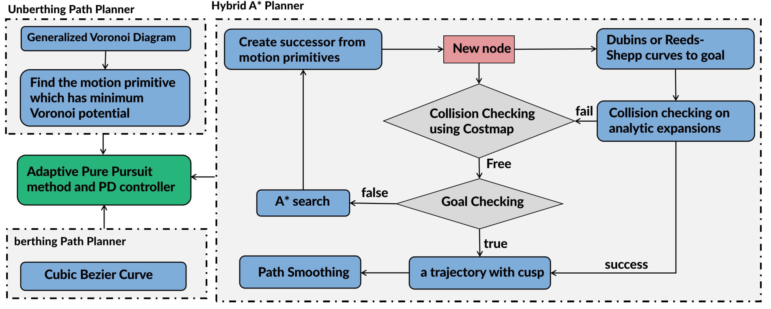
2.3. Path Planning at the Unberthing Phase

The unberthing phase involves the movement from the confined space to freer waters. We use the GVD for navigation during the unberthing phase. In order to generate the feasible path for vehicle with kinematic constraints, the motion primitives of the under-actuated vehicle are introduced, as shown in Figure 5. These motion primitives can be computed based on the maximum curvature and movement length. We exclude the motion primitives with high risk of collision and compute the Voronoi potential value of each movement based on GVD. The trajectory with the minimum potential value will be used to navigate the vehicle in the unberthing phase.

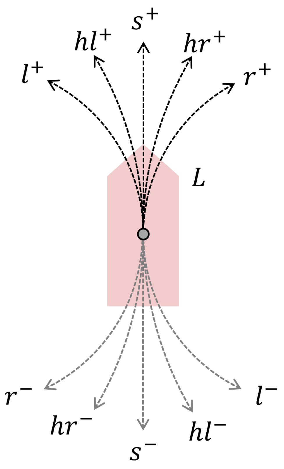
2.4. Hybrid A* Search Method

To ensure the kinematic feasibility and collision avoidance of the planned path, the four-dimensional search space is applied in hybrid A* search algorithm. Search with collision checking is also considered.

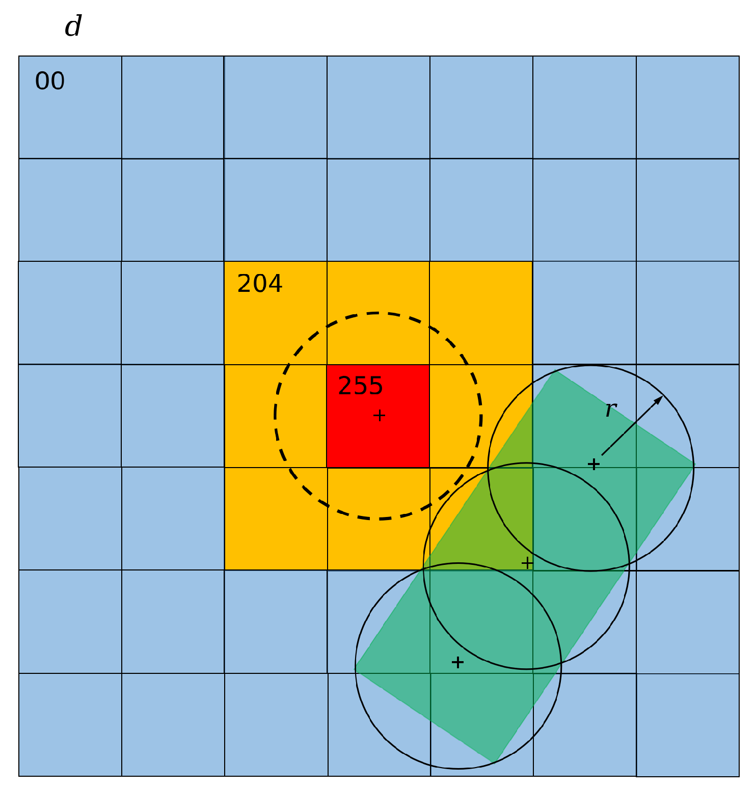
2.4.1. Costmap and Single-Source Shortest Path (SSSP) Map

The costmap is used to represent the planning space around vehicle. It represents a map of environment as an evenly spaced field, often called a grid cell. Each grid cell has a value in the range [0, 255] that indicates the likelihood the cell contains an obstacle. Firstly, we decompose the vehicle shape into a set of circles with the same radius R, called the inflation radius. Then, the shape of obstacles is inflated by computing the smallest integer number not less than $R/d$. Figure 6 shows an example of obstacle inflation, where the grid cell in the center is specified by 255 and the cells completely enclosing the circle are specified by 204. After the costmap is generated, the collision check will be performed by checking whether the center points of overlapping circles lie on the inflated area. For instance, the vehicle pose in Figure 6 is considered in collision.

The costmap inflates the size of obstacles based on the inflation radius. Decreasing the inflation radius will lead to more precise collision checking. Increasing the inflation radius makes it possible for vehicle to maintain a safe distance from obstacles. However, a large inflation radius will overinflate the obstacles, which is undesirable for path planning in narrow waters. Figure 7a shows an example of costmap with a large inflation radius, where the narrow channel becomes unnavigable. In this paper, we present a novel costmap using adaptive inflation radius, where the inflation radius of each grid cell $(x,y)$ is determined based on the distance from grid cell to its nearest edge of the GVD $d_V(x,y)$. Figure 7c shows the costmap with the adaptive inflation radius, where the inflated areas are reduced around the narrow channel.

The 2D map of Single-Source Shortest Path (SSSP) consists of the distances of the shortest paths from the goal and all other vertices in the graph. It uses the costmap to compute the shortest distances by performing Dijkstra’s algorithm, ignoring the non-holonomic nature of vehicle. Figure 7b,d illustrate the maps of SSSP. The SSSP map will never overestimate the actual cost to reach the goal, meaning that it can be used as an admissible heuristic function for hybrid A* search.

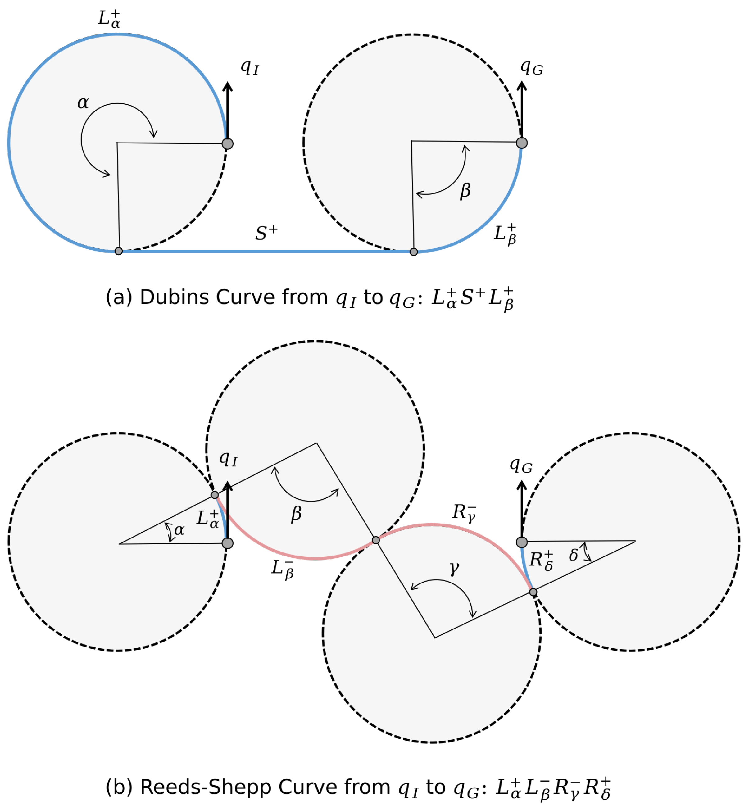
2.4.2. Dubins and Reeds–Shepp Curves

Dubins and Reeds-shepp curves (see Figure 8) are commonly used for non-holonomic vehicles, which are analytical methods to generate the optimal path in the two-dimensional plane [24]. With the curvature constraint on path, the Dubins path finds the shortest curve for forward-only vehicles that connects the initial pose and goal pose of vehicle. If the vehicle can also travel in reverse, then the optimal path follows the Reeds–Shepp curve [25].

2.4.3. Search Space Representation

The A* search extends its paths based on the cost of path $g\left(\mathrm{n}\right)$ and an admissible heuristic $h\left(\mathrm{n}\right)$ that estimates the cost to get to the goal state.

$$f\left(\mathrm{n}\right)=g\left(\mathrm{n}\right)+h\left(\mathrm{n}\right)$$

(9)

In the hybrid A* search, the path extension is achieved by a set of pre-computed motion primitives (see Figure 5). It means that the smallest entities of path extension are defined by arcs, which associates a continuous state with search space. The arc length L should be guaranteed to leave the current grid cell.

$$L>\sqrt{2}·d$$

(10)

The four-dimensional search space $(x,y,\phi ,d)$, including the location, orientation and direction of motion, are used to give an estimate of the cost of path. It applies higher penalties for traveling in the reverse direction and switching the direction of motion. The heuristic function in hybrid A* has been discussed above. During the node extension, the Dubins or Reeds–Shepp curves are computed from the current node to the goal. If these analytic curves are collision-free against the obstacles, the hybrid A* search will terminate.

2.5. Bézier Curve

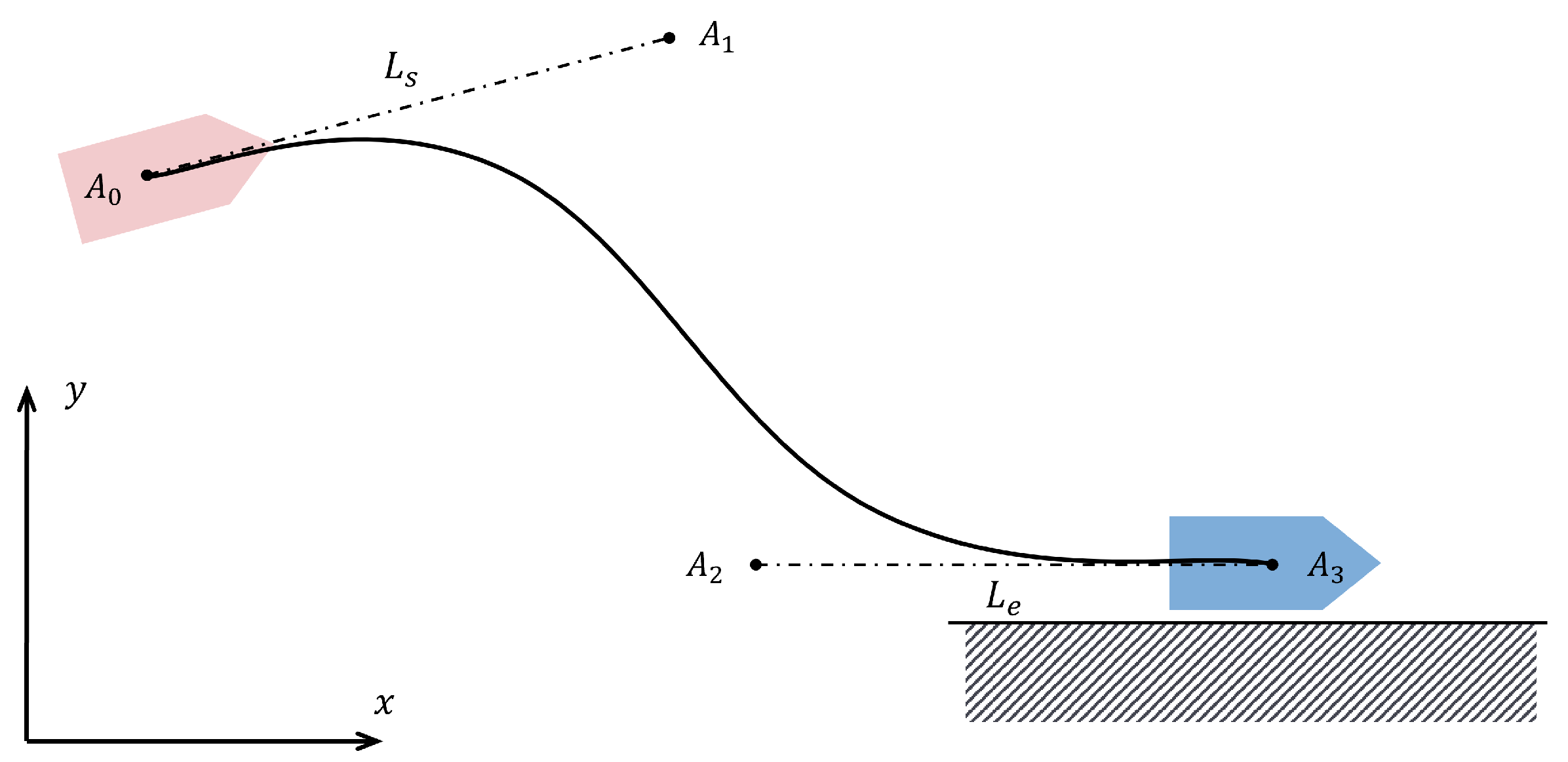
Due to the resolution of costmap and movement length in hybrid A* search, the search-based planner will never reach the exact goal pose of vehicle. To address this precision issue, we augment the search with analytic expansions based on a cubic Bézier curve [26].

$$B\left(t\right)={(1-t)}^3{A}_0+3t{(1-t)}^2{A}_1+3t^2(1-t)A_2+t^3{A}_3,0\le t\le 1$$

(11)

where the Bézier curve (see Figure 1) is defined by four points, $A_0,A_1,A_2,A_3$, in the plane. The point $A_0$ is the goal of hybrid A* search planner. The $A_3$ is placed at the berthing position, where the orientation of line segment $A_2{A}_3$ is the same as the berthing orientation. The adjustment of lengths $L_s$ and $L_e$ leads to a smooth berthing trajectory for the vehicle to follow. Such a Bézier-based planner is appropriate only under the assumption that the environment around the berthing position is collision-free.

2.6. Path-Following Method

The path-following algorithm makes the vehicle follow the target path smoothly and accurately. In this paper, the adaptive pure pursuit algorithm is used to generate the target course for the ASV. As shown in Figure 9, the target point can be determined by finding the first point on the target path whose distance to vehicle is larger than the look-ahead distance $L_T$. The adaptive look-ahead distance $L_T$ will vary with the curvature of target path. When the vehicle goes around a sharp turn, look-ahead distance will be reduced. The course error ${\theta }_T$ can be computed based on the target point on the target path. A PD controller is applied to compute the thruster command based on the speed and course error. The proposed path-following method ensures the performance to control a ship with sufficient precision.

2.7. Architecture of Automatic Berthing Algorithm

The architecture of path-planning algorithm for automatic berthing operation is illustrated in Figure 10. If the hybrid A* search planner fails to compute a feasible path, the unberthing path planner will be activated, which makes the vehicle move toward open waters. After the unberthing phase is finished, the hybrid A* search planner re-computes a smooth and collision-free path from the current pose to the goal. Combined with the Bézier curve, the automatic berthing algorithm provides a safe trajectory with high precision.

3. Case Study: Simulations and Field Trials

The case study on two types of berthing operations (see Figure 11) is presented in this paper. The berthing precision is defined as follows.

$$P_b=max\left(\frac{\left|d\right|}{\widehat{d}},\frac{\left|\theta -{\theta }_d\right|}{\widehat{\theta }},\frac{\left|u\right|}{\widehat{u}}\right)$$

(12)

where $\left|d\right|$ and $\widehat{d}$ denote the tracking error and the maximum allowed tracking error, $\left|\theta -{\theta }_d\right|$ represents the heading error between the real-time and target heading angle, and $\widehat{\theta }$ denotes the maximum allowed heading error. $\left|u\right|$ and $\widehat{u}$ denote the vehicle speed and the maximum allowed speed. If $P_b<1.0$, it means the berthing precision is satisfactory. For the perpendicular dock, $\widehat{d}=1.0\mathrm{m},\widehat{\theta }=0.05\mathrm{rad},\widehat{u}=0.4\mathrm{m}/\mathrm{s}$. For the parallel dock, $\widehat{d}=0.2\mathrm{m},\widehat{\theta }=0.1\mathrm{rad},\widehat{u}=0.4\mathrm{m}/\mathrm{s}$.

We used the following parameters for the berthing planner: the costmap and hybrid A* search use the size $200\mathrm{m}\times 200\mathrm{m}$ with a $0.5\mathrm{m}$ resolution. The proposed algorithms, including the path-planning, path-following and control, are implemented on a computer with an ARM 1.8 GHz CPU. We maintained the costmap and GVD at every iteration of the hybrid A* search, whose run time was on the order of 30–200 ms. The parameters in PD heading controller $K_p=300, K_d=200$ are set, and the look-ahead distance in the pure pursuit algorithm is 4.5 m.

3.1. Simulation Results

The berthing simulation was performed with the 3DoF model of the vehicle. The environmental disturbances are not considered in the simulation. The simulation results are illustrated in Figure 12, Figure 13 and Figure 14, where the blue dotted line represents the target path generated by the proposed path planner, and the black triangles indicate the simulated poses of vehicle. The green and red triangles indicate the initial pose and berthing pose.

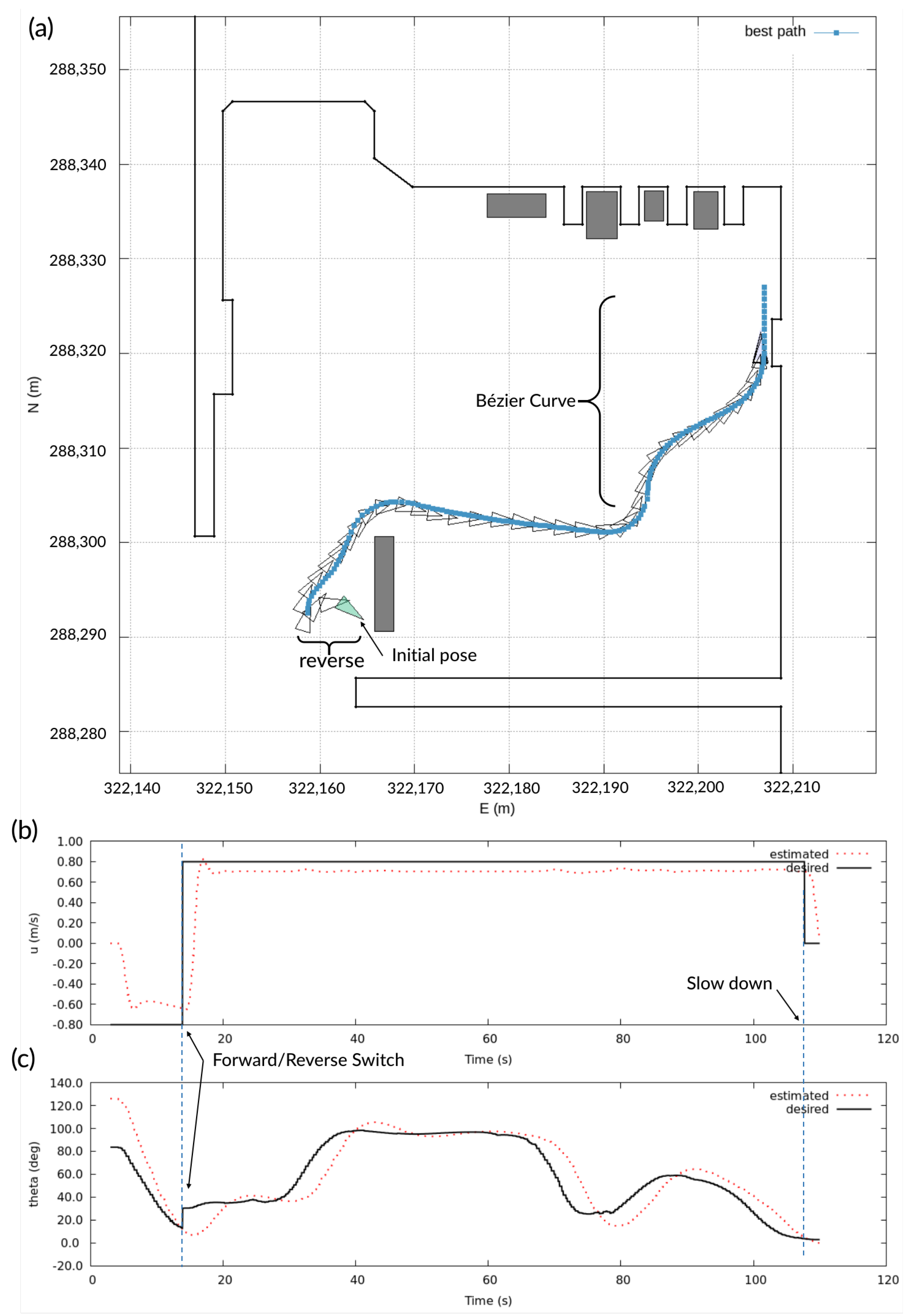
3.1.1. Case 01

In test case 01, the initial position of the vehicle is very close to the obstacle (see Figure 12a). Firstly, the vehicle performs the reversing maneuvers based on the unberthing planner, as shown in Figure 12b. When the reverse path is completed, it regenerates a collision-free path toward the berthing position. Such a path maintains a safe distance from obstacles. The final berthing operation is guided by the Bézier curve with $L_s=L_e=10\mathrm{m}$. It achieves a desirable berthing precision ($P_b=0.58$), with $\left|d\right|=0.013\mathrm{m}, \left|\theta -{\theta }_d\right|=0.007\mathrm{rad},$ $\left|u\right|=0.23\mathrm{m}/\mathrm{s}$ at the time $t=109\mathrm{s}$.

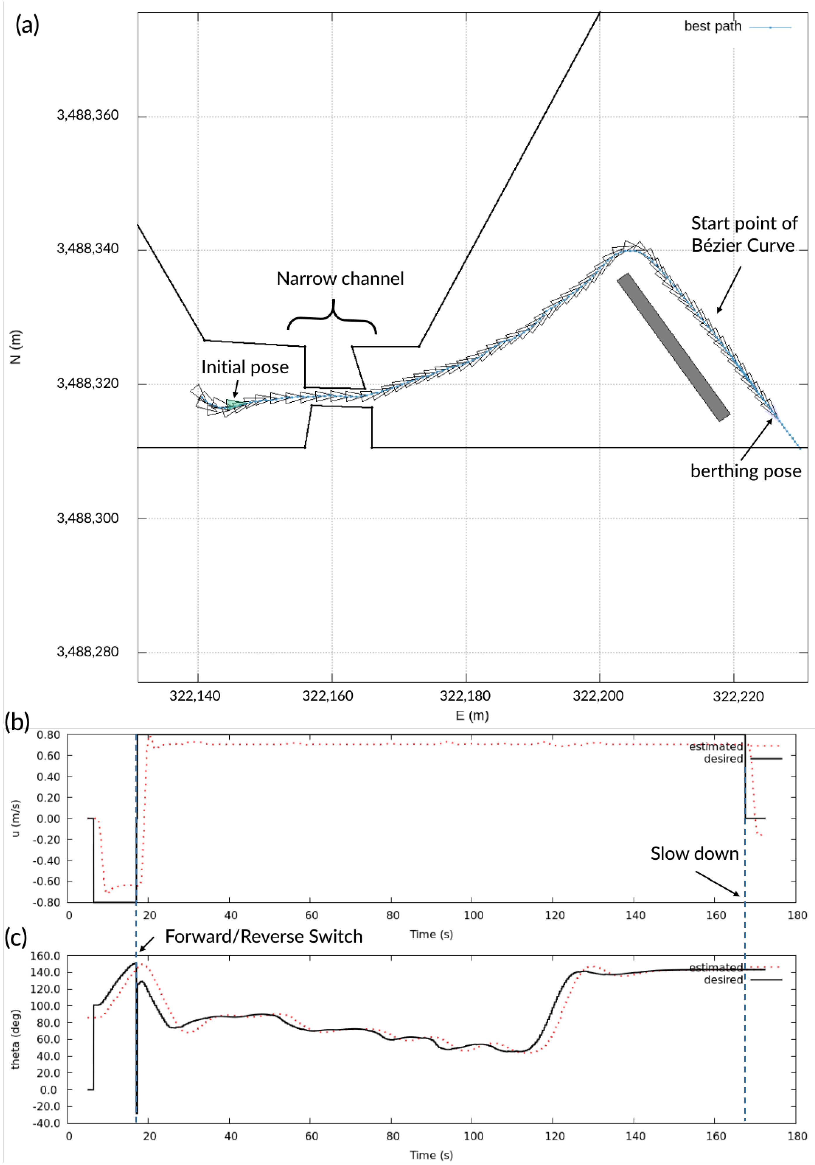
3.1.2. Case 02

In the test case 02, the initial vehicle’s direction is almost opposite to the berthing direction (see Figure 13). The vehicle generates a target path, a concatenation of the hybrid A* result and Bézier curve, without switching the direction of motion. This demonstrates the advantage of the Bézier curve. Furthermore, the adaptive pure pursuit method ensures desirable tracking performance, which leads to a good balance in terms of berthing precision and comfortable movement. At the time $t=88\mathrm{s}$, it achieves a desirable berthing precision ($P_b=0.45$), with $\left|d\right|=0.002\mathrm{m}, \left|\theta -{\theta }_d\right|=0.011\mathrm{rad}, \left|u\right|=0.18\mathrm{m}/\mathrm{s}$.

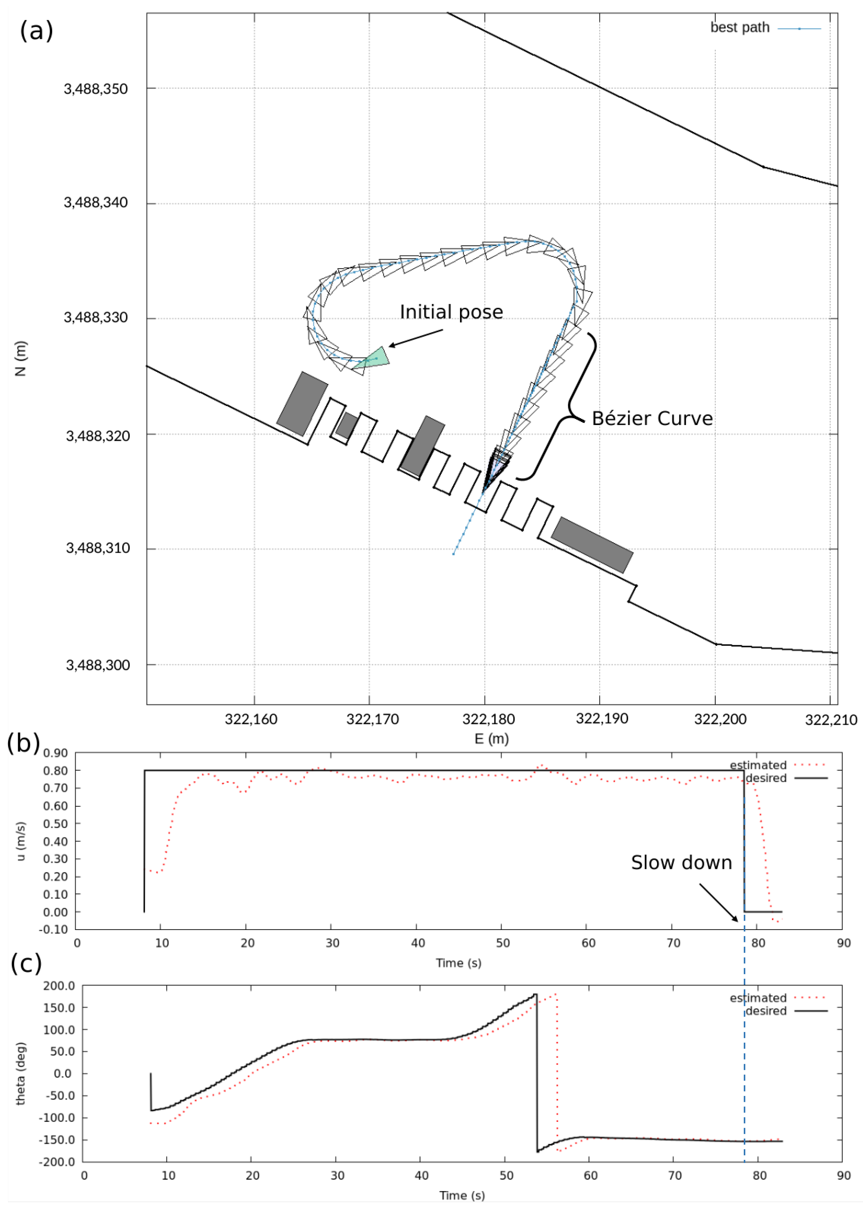
3.1.3. Case 03

In the test case 03, the vehicle must generate a feasible path in the narrow channel, whose minimum width is 2.7 m. A box-shaped obstacle is placed in front of the berthing position in order to increase the complexity of the path planning. As shown in Figure 14, the vehicle firstly fails to compute a safe navigation path within the narrow channel. Then, it moves in the reverse direction based on the unberthing planner. When the unberthing path is finished, the vehicle recomputes a smooth path that safely navigates within the narrow channel. After the vehicle crosses the narrow channel, it bypasses the obstacle and keeps a comfortable distance from the obstacle around the corner. At the time $t=110\mathrm{s}$, it achieves a desirable berthing precision ($P_b=0.5$), with $\left|d\right|=0.003\mathrm{m}, \left|\theta -{\theta }_d\right|=0.009\mathrm{rad}, \left|u\right|=0.21\mathrm{m}/\mathrm{s}$.

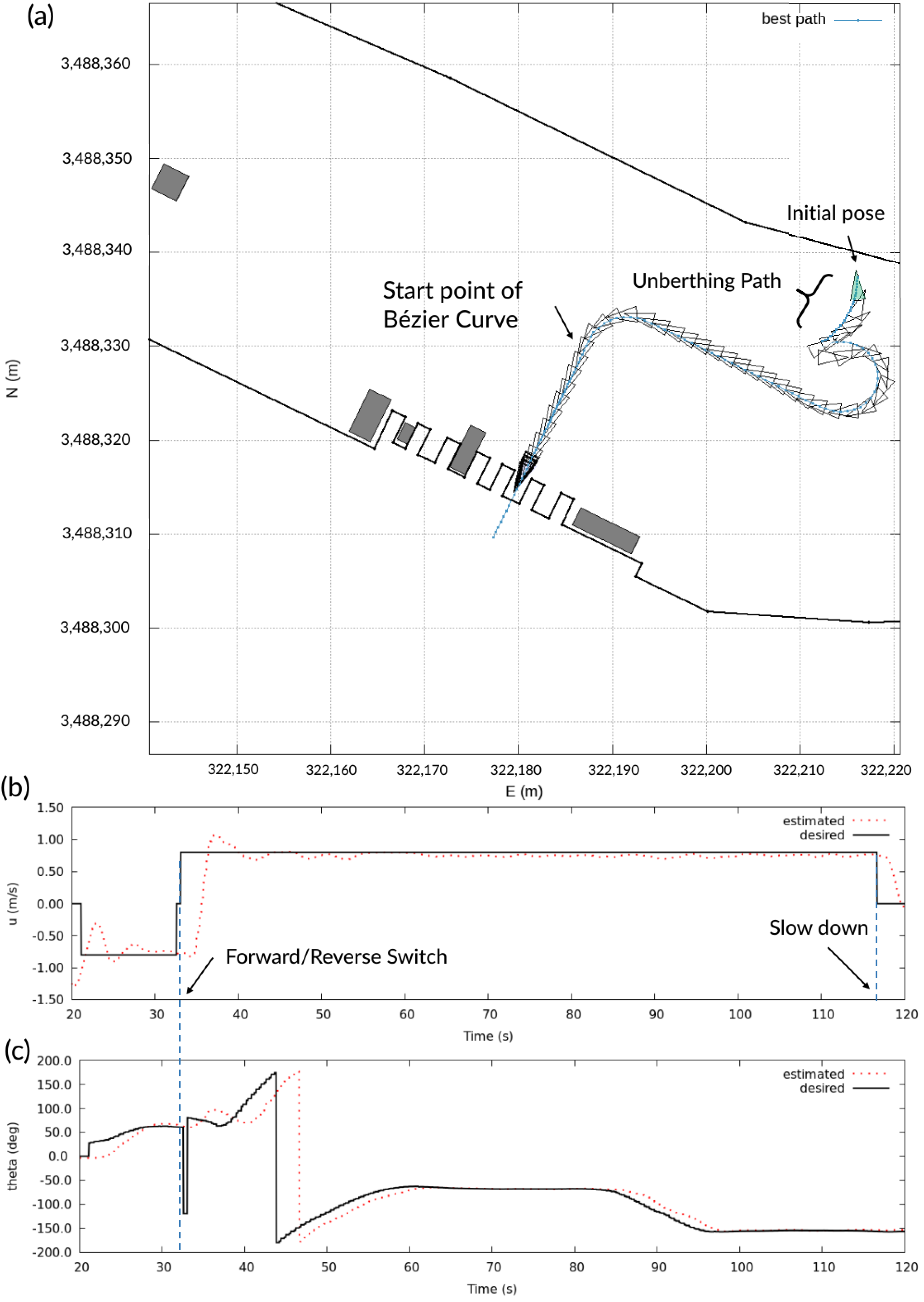
3.2. Experimental Results

The experiment was developed on a catamaran (see Figure 2) by integrating the GNSS sensor, thrusters, wireless modem, batteries, etc. The GNSS sensor with the Continuously Operating Reference Station (CORS) provides the positioning, heading and velocity of the vehicle, with a positioning accuracy of 0.05 m and heading accuracy of 0.1 degree. We tested the planning and tracking capabilities under calm waters. The experimental results are illustrated in the figures, where the blue dotted line represents the target path, the GNSS-measured poses of the vehicle are described by black triangles, and the initial pose and berthing pose are represented by green and blue triangles, respectively.

3.2.1. Case 04

The perpendicular dock is set up in test case 04. The initial pose of the vehicle is close to the surrounding obstacles. However, Figure 15 shows that the vehicle generates a smooth path with the positive target speed, as the planner applies a penalty for driving in reverse. For the Bézier curve, the distance between the starting point ($A_0$) and berthing point ($A_3$) is 18 m in order to ensure sufficient precision in the tracking error and heading angle, especially when the vehicle begins to enter the dock. At the time $t=82\mathrm{s}$, it achieves a desirable berthing precision ($P_b=0.5$), with $\left|d\right|=0.005\mathrm{m}, \left|\theta -{\theta }_d\right|=0.025\mathrm{rad}, \left|u\right|=0.08\mathrm{m}/\mathrm{s}$.

3.2.2. Case 05

Figure 16 shows the results of test cast 05. Firstly, the vehicle is required to travel in reverse, as the forward movement has a high risk of collision with obstacles. There is a large tracking error between the vehicle and target path at the moment when the vehicle experiences a change in the direction of motion. These errors become small as the vehicle travels toward the berthing position. At the time $t=114\mathrm{s}$, it achieves a desirable berthing precision ($P_b=0.8$), with $\left|d\right|=0.08\mathrm{m}, \left|\theta -{\theta }_d\right|=0.002\mathrm{rad}, \left|u\right|=0.07\mathrm{m}/\mathrm{s}$.

3.2.3. Case 06

Figure 17 shows the successful unberthing and berthing operation in the test case 06. At first, it fails to compute a feasible path using the hybrid A* search method. Therefore, the vehicle generates the unberthing path with the negative target speed at the time duration from 22 s to 33 s (see Figure 17b). Once the unberthing operation is finished, the planning module succeeds at generating a smooth path using the hybrid A* search. At the time $t=119\mathrm{s}$, it achieves a desirable berthing precision ($P_b=0.5$), with $\left|d\right|=0.05\mathrm{m},$ $\left|\theta -{\theta }_d\right|=0.002\mathrm{rad}, \left|u\right|=0.06\mathrm{m}/\mathrm{s}$.

4. Conclusions

We propose a graph search-based path-planning method for the automatic ship berthing operation. This process can be divided into two phases: transit and berthing. The transit phase utilizes the hybrid A* search planner to generate a smooth and collision-free path. The efficiency of such a search can be improved using the adaptive costmap and SSSP based on the GVD of the surrounding obstacles. The berthing phase applies the cubic Bézier curve for the final berthing operation. It enables safer operation through gentle and precise control. The simulation and experimental results successfully demonstrate the performance of the proposed path-planning strategy in terms of its safety and berthing precision. Extensive experimental research should be conducted on the application of simultaneous localization and mapping (SLAM) in the automatic berthing system, which will increase the levels of autonomy.

References

- Ohtsu, K.; Takai, T.; Yoshihisa, H. A Fully Automatic Berthing Test Using the Training Ship Shioji Maru. J. Navig. 1991, 44, 213–223. [Google Scholar] [CrossRef]
- Djouani, K.; Hamam, Y. Minimum time-energy trajectory planning for automatic ship berthing. IEEE J. Ocean. Eng. 1995, 20, 4–12. [Google Scholar] [CrossRef]
- Maki, A.; Sakamoto, N.; Akimoto, Y.; Nishikawa, H.; Umeda, N. Application of optimal control theory based on the evolution strategy (CMA-ES) to automatic berthing. J. Mar. Sci. Technol. 2020, 25, 221–233. [Google Scholar] [CrossRef]
- Mizuno, N.; Uchida, Y.; Okazaki, T. Quasi Real-Time Optimal Control Scheme for Automatic Berthing. IFAC-PapersOnLine 2015, 48, 305–312. [Google Scholar] [CrossRef]
- Ahmed, Y.A.; Hasegawa, K. Automatic Ship Berthing using Artificial Neural Network Based on Virtual Window Concept in Wind Condition. IFAC Proc. Vol. 2012, 45, 286–291. [Google Scholar] [CrossRef]
- Ahmed, Y.A.; Hasegawa, K. Automatic ship berthing using artificial neural network trained by consistent teaching data using nonlinear programming method. Eng. Appl. Artif. Intell. 2013, 26, 2287–2304. [Google Scholar] [CrossRef]
- Wang, S.; Sun, Z.; Yuan, Q.; Sun, Z.; Wu, Z.; Hsieh, T.H. Autonomous piloting and berthing based on Long Short Time Memory neural networks and nonlinear model predictive control algorithm. Ocean Eng. 2022, 264, 112269. [Google Scholar] [CrossRef]
- Shuai, Y.; Li, G.; Cheng, X.; Skulstad, R.; Xu, J.; Liu, H.; Zhang, H. An efficient neural-network based approach to automatic ship docking. Ocean Eng. 2019, 191, 106514. [Google Scholar] [CrossRef]
- Skulstad, R.; Li, G.; Fossen, T.I.; Vik, B.; Zhang, H. A Hybrid Approach to Motion Prediction for Ship Docking—Integration of a Neural Network Model Into the Ship Dynamic Model. IEEE Trans. Instrum. Meas. 2021, 70, 1–11. [Google Scholar] [CrossRef]
- Martinsen, A.B.; Lekkas, A.M.; Gros, S. Autonomous docking using direct optimal control. IFAC-PapersOnLine 2019, 52, 97–102. [Google Scholar] [CrossRef]
- Miyauchi, Y.; Sawada, R.; Akimoto, Y.; Umeda, N.; Maki, A. Optimization on planning of trajectory and control of autonomous berthing and unberthing for the realistic port geometry. Ocean Eng. 2022, 245, 110390. [Google Scholar] [CrossRef]
- Martinsen, A.B.; Bitar, G.; Lekkas, A.M.; Gros, S. Optimization-Based Automatic Docking and Berthing of ASVs Using Exteroceptive Sensors: Theory and Experiments. IEEE Access 2020, 8, 204974–204986. [Google Scholar] [CrossRef]
- Shimizu, S.; Nishihara, K.; Miyauchi, Y.; Wakita, K.; Suyama, R.; Maki, A.; Shirakawa, S. Automatic berthing using supervised learning and reinforcement learning. Ocean Eng. 2022, 265, 112553. [Google Scholar] [CrossRef]
- González, D.; Pérez, J.; Milanés, V.; Nashashibi, F. A Review of Motion Planning Techniques for Automated Vehicles. IEEE Trans. Intell. Transp. Syst. 2016, 17, 1135–1145. [Google Scholar] [CrossRef]
- Dolgov, D.A. Practical Search Techniques in Path Planning for Autonomous Driving; American Association for Artificial Intelligence: Washington, DC, USA, 2008. [Google Scholar]
- Dolgov, D.; Thrun, S.; Montemerlo, M.; Diebel, J. Path Planning for Autonomous Driving in Unknown Environments. In Experimental Robotics; Springer: Berlin/Heidelberg, Germany, 2009; pp. 55–64. [Google Scholar]
- Bitar, G.; Martinsen, A.B.; Lekkas, A.M.; Breivik, M. Two-Stage Optimized Trajectory Planning for ASVs Under Polygonal Obstacle Constraints: Theory and Experiments. IEEE Access 2020, 8, 199953–199969. [Google Scholar] [CrossRef]
- Reeds, J.; Shepp, L. Optimal paths for a car that goes both forwards and backwards. Pac. J. Math. 1990, 145, 367–393. [Google Scholar] [CrossRef]
- Fossen, T.I. Handbook of Marine Craft Hydrodynamics and Motion Control; John Wiley & Sons: Hoboken, NJ, USA, 2011. [Google Scholar]
- Wirtensohn, S.; Reuter, J.; Blaich, M.; Schuster, M.; Hamburger, O. Modelling and identification of a twin hull-based autonomous surface craft. In Proceedings of the 2013 18th International Conference on Methods and Models in Automation and Robotics (MMAR), Miedzyzdroje, Poland, 26–29 August 2013; pp. 121–126. [Google Scholar] [CrossRef]
- Hu, Z.; Yang, Z.; Zhang, W. Path planning for auto docking of underactuated ships based on Bezier curve and hybrid A* search algorithm. Chin. J. Ship Res. 2024, 19, 220–229. [Google Scholar] [CrossRef]
- Fortune, S. A sweepline algorithm for Voronoi diagrams. In Proceedings of the Second Annual Symposium on Computational Geometry, Yorktown Heights, NY, USA, 2–4 June 1986; pp. 313–322. [Google Scholar]
- Masehian, E.; Amin-Naseri, M. A voronoi diagram-visibility graph-potential field compound algorithm for robot path planning. J. Robot. Syst. 2004, 21, 275–300. [Google Scholar] [CrossRef]
- LaValle, S.M. Planning Algorithms; Cambridge University Press: Cambridge, UK, 2006. [Google Scholar]
- Sucan, I.A.; Moll, M.; Kavraki, L.E. The open motion planning library. IEEE Robot. Autom. Mag. 2012, 19, 72–82. [Google Scholar] [CrossRef]
- Marcucci, T.; Nobel, P.; Tedrake, R.; Boyd, S. Fast Path Planning Through Large Collections of Safe Boxes. arXiv 2024, arXiv:2305.01072. [Google Scholar]