
Non-Equilibrium Scour Evolution around an Emerged Structure Exposed to a Transient Wave

Abstract
:1. Introduction
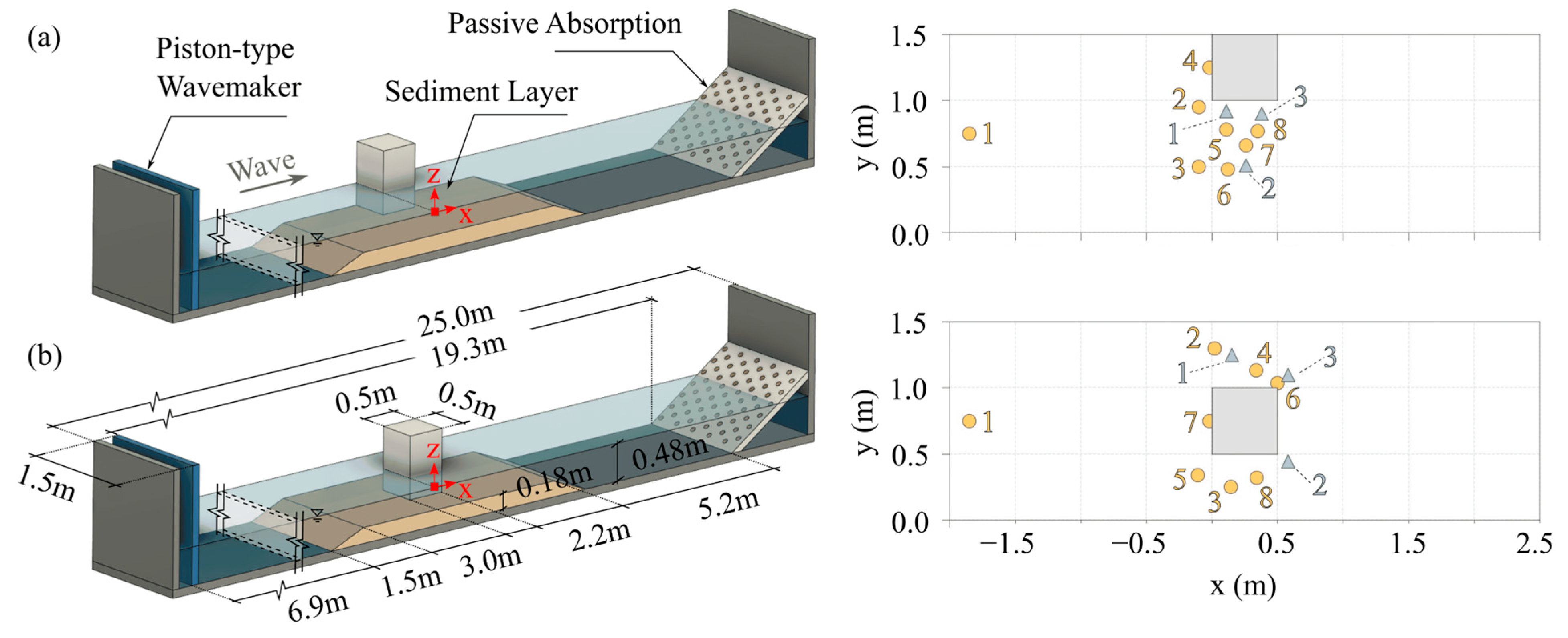
2. Physical Modeling
3. Numerical Modeling
3.1. SedWaveFoam
3.2. FLOW-3D
3.3. Implementation
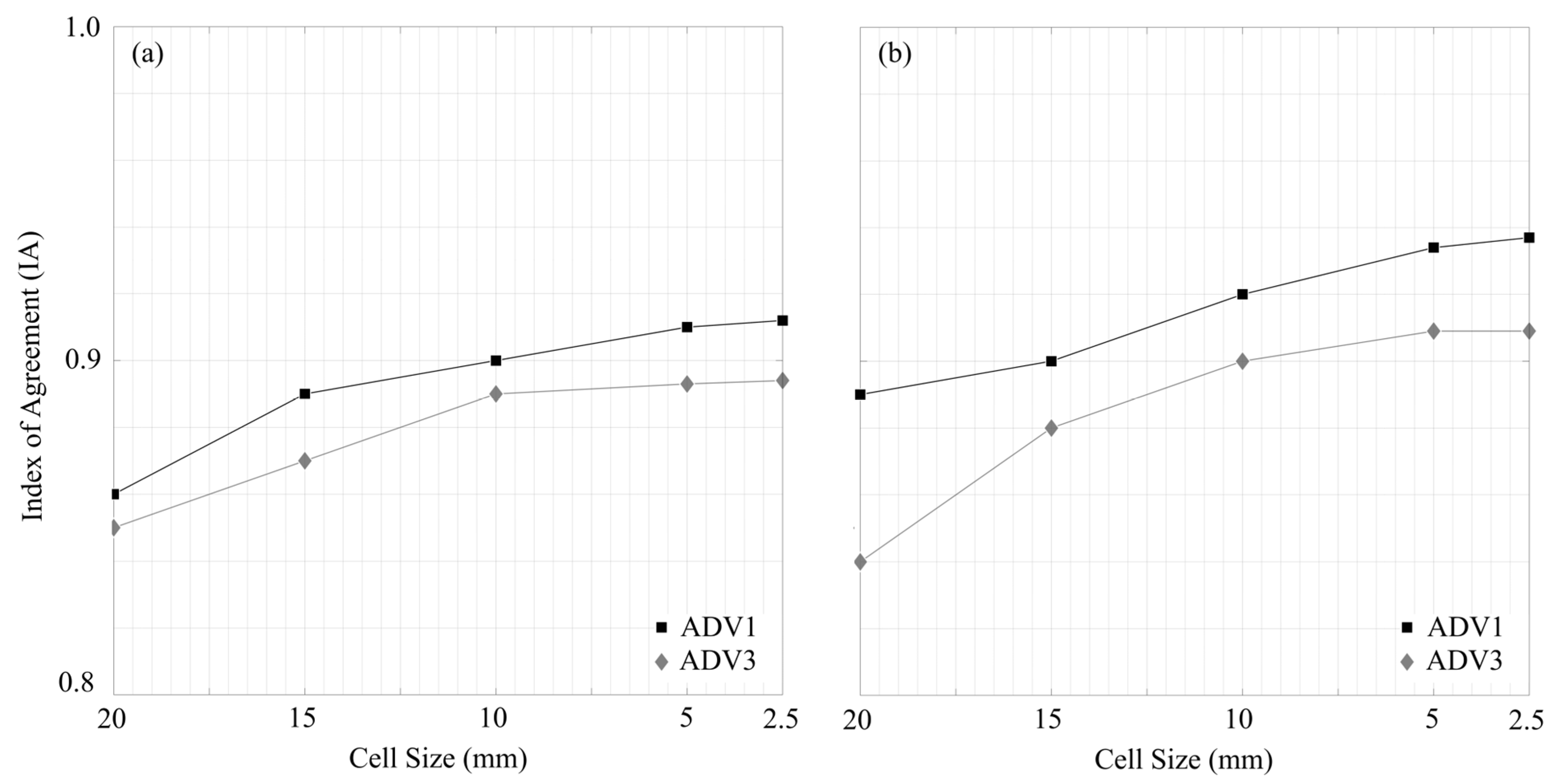
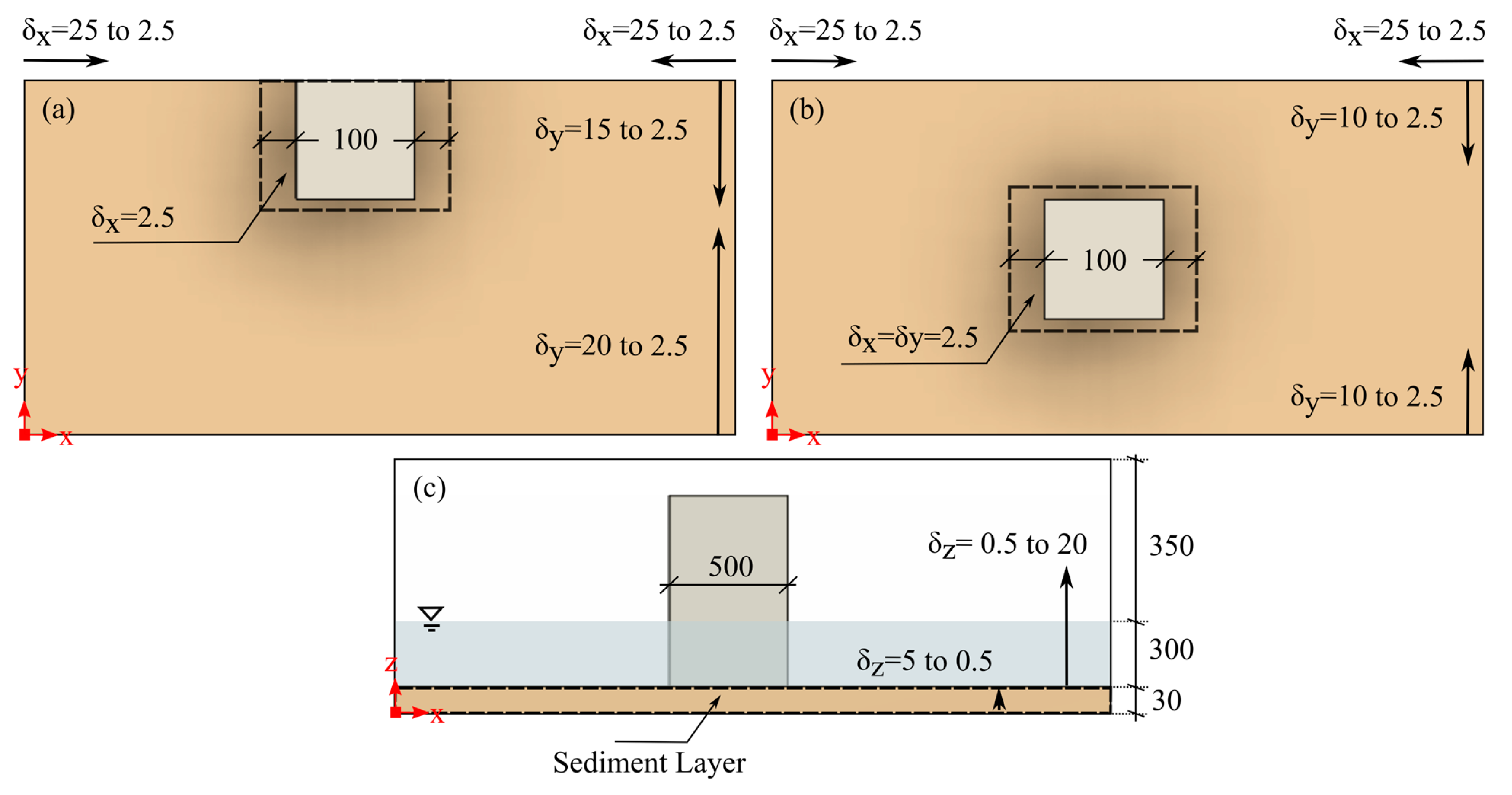
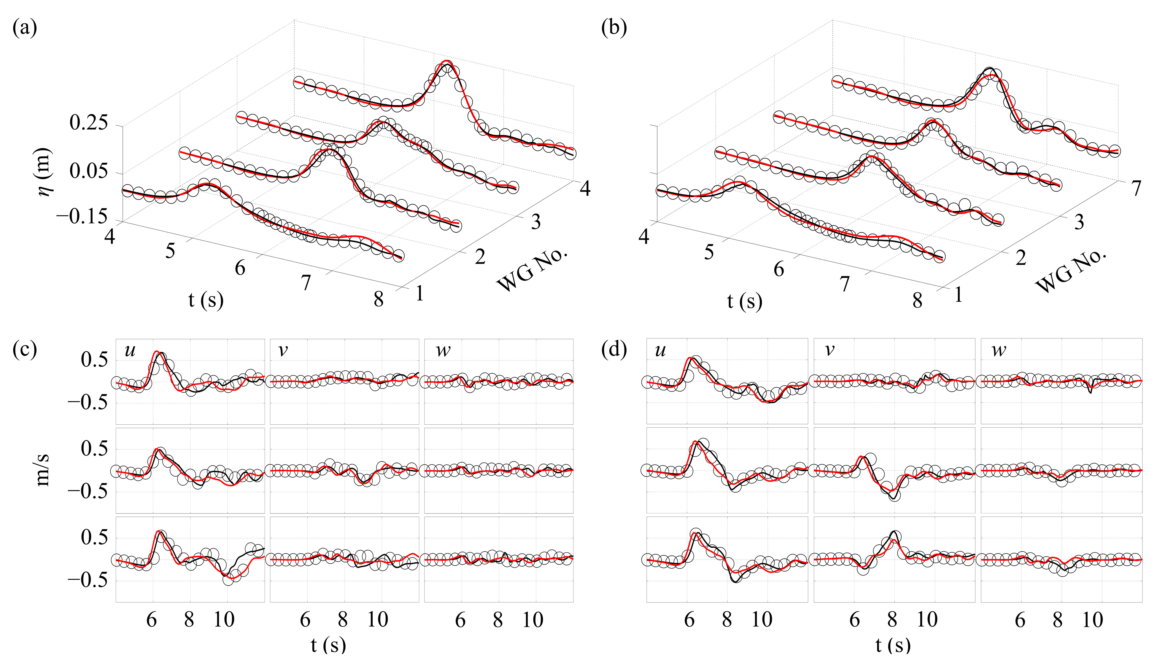
3.4. Validation
3.5. Model Calibration
3.5.1. Entrainment Parameter
3.5.2. Bedload Transport Model
3.5.3. Turbulence Scheme
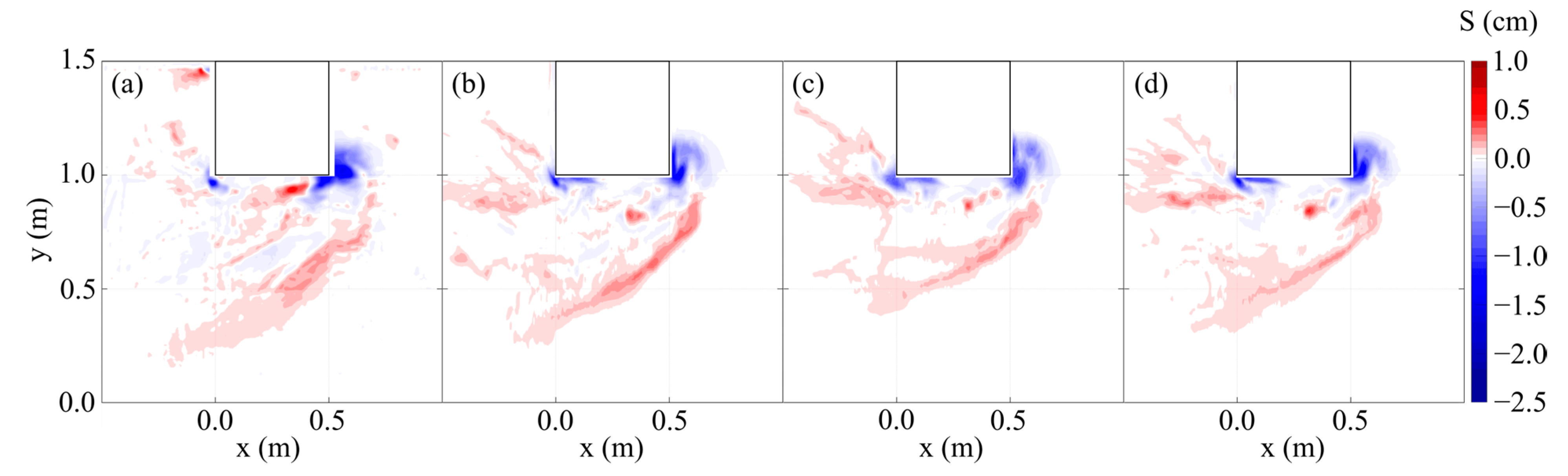
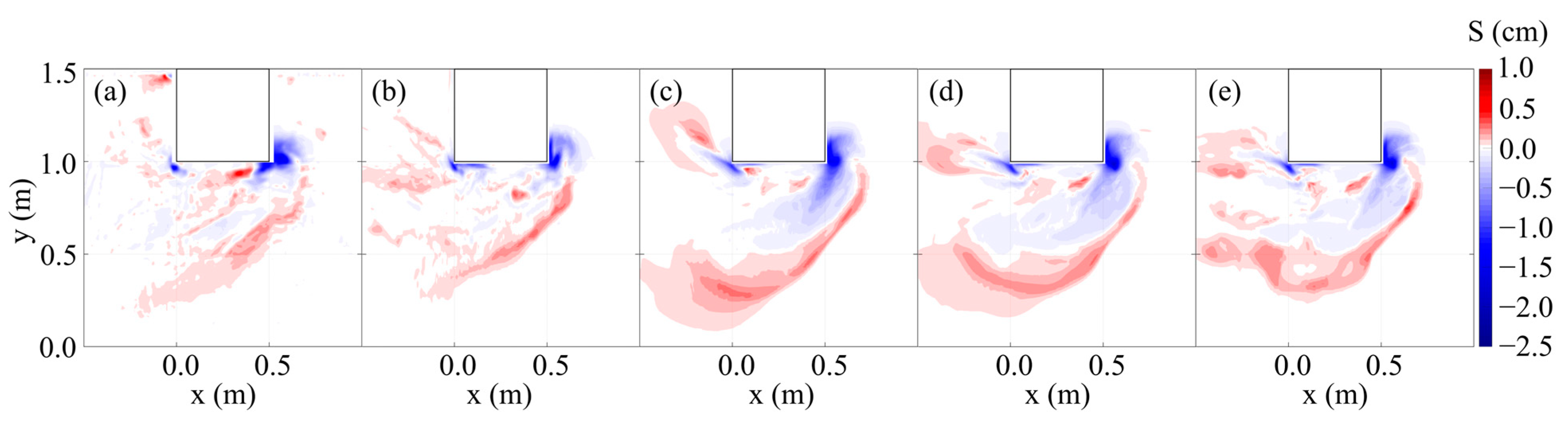
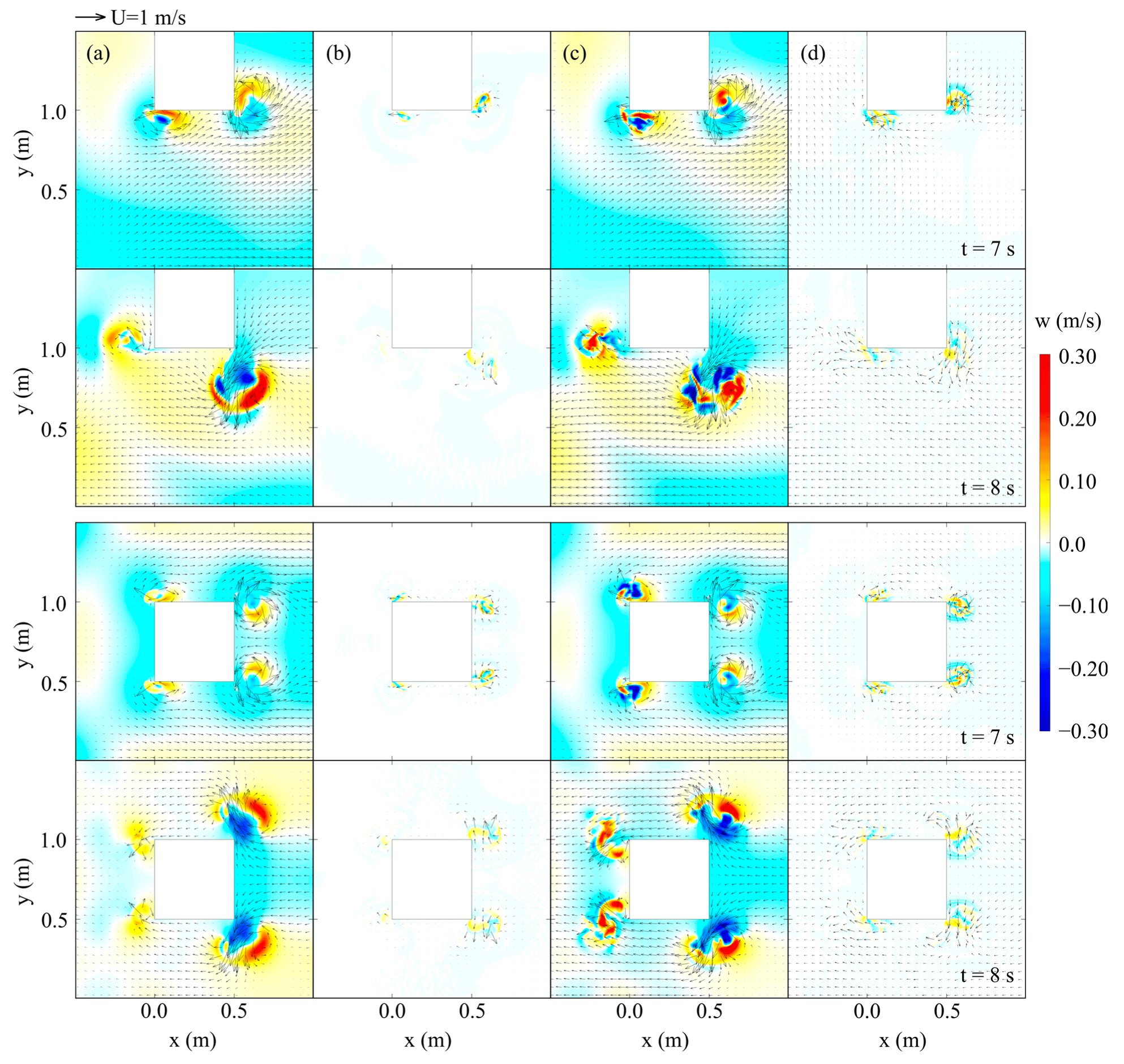
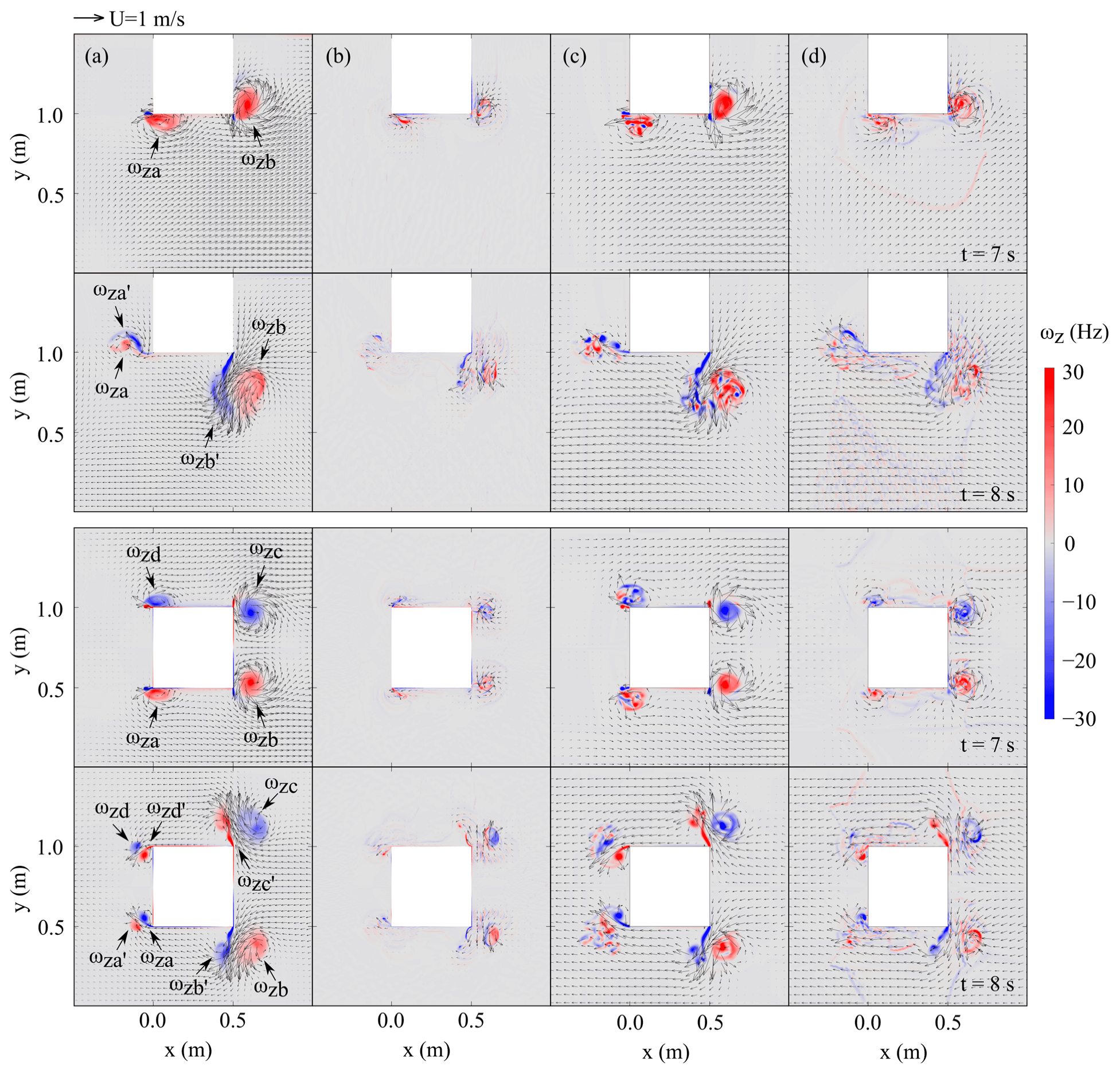
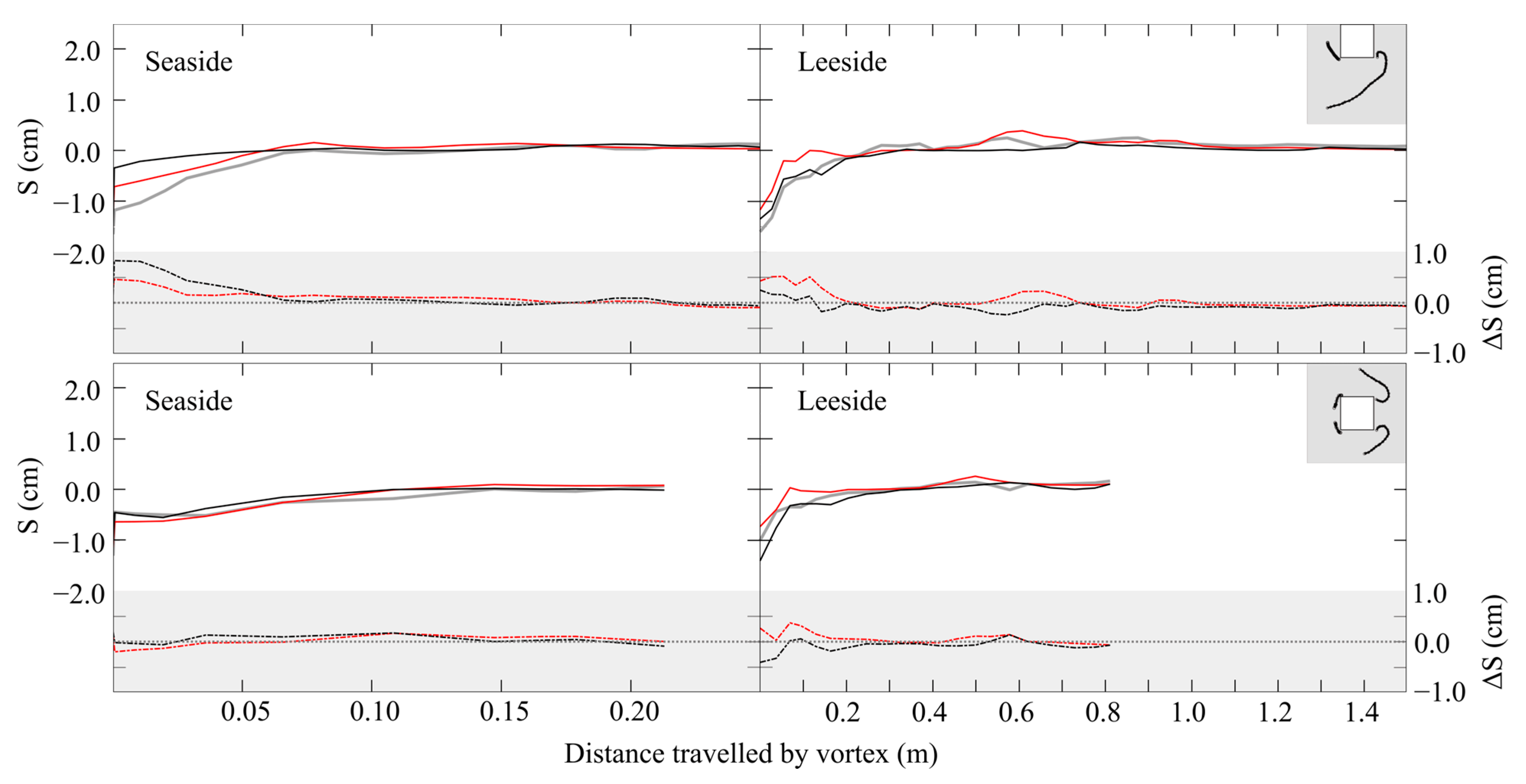
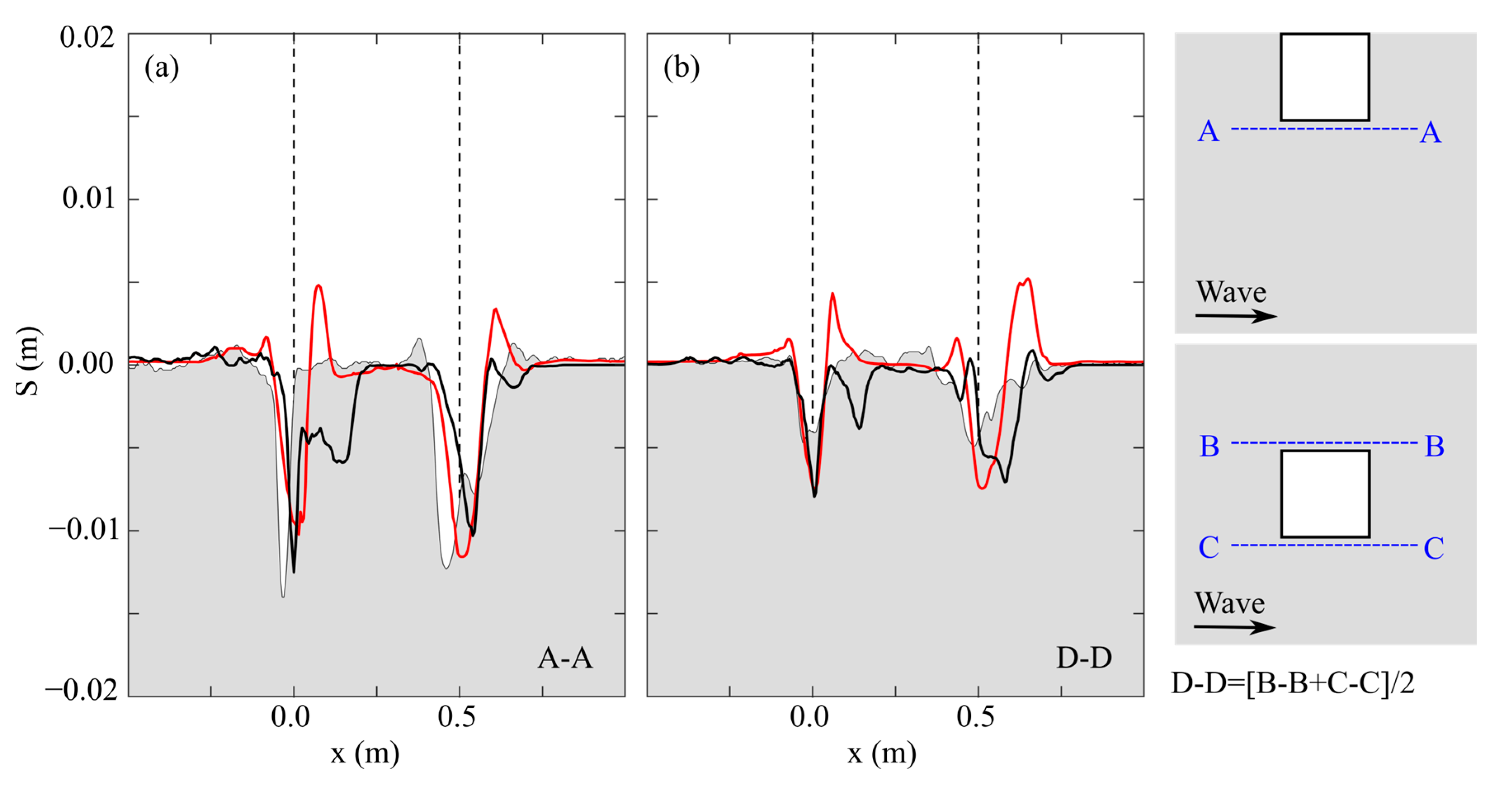
4. Results and Discussion
5. Conclusions
Author Contributions
Funding
Institutional Review Board Statement
Informed Consent Statement
Data Availability Statement
Acknowledgments
Conflicts of Interest
References
- Larsen, B.E.; Fuhrman, D.R.; Baykal, C.; Sumer, B.M. Tsunami-induced scour around monopile foundations. Coast. Eng. 2017, 129, 36–49. [Google Scholar] [CrossRef]
- Williams, I.A.; Fuhrman, D.R. Numerical simulation of tsunami-scale wave boundary layers. Coast. Eng. 2016, 110, 17–31. [Google Scholar] [CrossRef]
- Breusers, H.N.C.; Nicollet, G.; Shen, H. Local scour around cylindrical piers. J. Hydraul. Res. 1977, 15, 211–252. [Google Scholar] [CrossRef]
- Carreiras, J.; Larroudé, P.; Seabra-Santos, F.; Mory, M. Wave scour around piles. In Proceedings of the 27th International Conference on Coastal Engineering 2000, Sydney, Australia, 16–21 July 2000; pp. 1860–1870. [Google Scholar]
- Carreiras, J.; Carmo, J.D.; Seabra-Santos, F. Settlement of vertical piles exposed to waves. Coast. Eng. 2003, 47, 355–365. [Google Scholar] [CrossRef]
- Dey, S.; Sumer, B.M.; Fredsøe, J. Control of scour at vertical circular piles under waves and current. J. Hydraul. Eng. 2006, 132, 270–279. [Google Scholar] [CrossRef]
- Dey, S.; Helkjær, A.; Sumer, B.M.; Fredsøe, J. Scour at vertical piles in sand-clay mixtures under waves. J. Waterw. Port Coast. Ocean Eng. 2011, 137, 324–331. [Google Scholar] [CrossRef]
- Kobayashi, T. 3-D Analysis of flow around a vertical cylinder on a scoured bed. In Proceedings of the 23rd International Conference on Coastal Engineering, Venice, Italy, 4–9 October 1992; pp. 3482–3495. [Google Scholar]
- Kobayashi, T.; Oda, K. Experimental study on developing process of local scour around a vertical cylinder. In Proceedings of the 24th International Conference on Coastal Engineering, Kobe, Japan, 23 October 1994; pp. 1284–1297. [Google Scholar] [CrossRef]
- Raaijmakers, T.; Rudolph, D. Time-dependent scour development under combined current and waves conditions-laboratory experiments with online monitoring technique. In Proceedings of the 4th International Conference on Scour and Erosion, ICSE, Tokyo, Japan, 5–7 November 2008; pp. 152–161. [Google Scholar]
- Sumer, B.M.; Christiansen, N.; Fredsoe, J. Time scale of scour around a vertical pile. In Proceedings of the ISOPE International Ocean and Polar Engineering Conference, San Francisco, CA, USA, 14–19 June 1992; p. ISOPE-I-92-259. [Google Scholar]
- Sumer, B.M.; Fredsøe, J.; Christiansen, N. Scour around vertical pile in waves. J. Waterw. Port Coast. Ocean Eng. 1992, 118, 15–31. [Google Scholar] [CrossRef]
- Sumer, B.M.; Christiansen, N.; Fredsøe, J. Influence of cross section on wave scour around piles. J. Waterw. Port Coast. Ocean Eng. 1993, 119, 477–495. [Google Scholar] [CrossRef]
- Sumer, B.M.; Fredsøe, J.; Christiansen, N.; Hansen, S.B. Bed shear stress and scour around coastal structures. In Proceedings of the 24th International Conference on Coastal Engineering, Kobe, Japan, 23 October 1994; pp. 1595–1609. [Google Scholar]
- Sumer, B.M.; Fredsøe, J. Scour around pile in combined waves and current. J. Hydraul. Eng. 2001, 127, 403–411. [Google Scholar] [CrossRef]
- Sumer, B.M.; Fredsøe, J. Time scale of scour around a large vertical cylinder in waves. In Proceedings of the ISOPE International Ocean and Polar Engineering Conference, Kitakyushu, Japan, 26–31 May 2002; p. ISOPE-I-02-143. [Google Scholar]
- Sumer, B.M.; Fredsøe, J. The mechanics of scour in the marine environment. In Advanced Series on Ocean Engineering; Word Scientific: Singapore, 2002. [Google Scholar]
- Sumer, B.M. Mathematical modelling of scour: A review. J. Hydraul. Res. 2007, 45, 723–735. [Google Scholar] [CrossRef]
- Whitehouse, R. Scour at Marine Structures: A Manual for Practical Applications; Thomas Telford: London, UK, 1998. [Google Scholar]
- Zanke, U.C.; Hsu, T.-W.; Roland, A.; Link, O.; Diab, R. Equilibrium scour depths around piles in noncohesive sediments under currents and waves. Coast. Eng. 2011, 58, 986–991. [Google Scholar] [CrossRef]
- Rance, P.J. The Potential for Scour around Large Objects, One-Day Seminar of Scour Prevention Techniques around Offshore Structures; Society for Underwater Technology: London, UK, 1980; p. 41. [Google Scholar]
- Nakamura, T.; Kuramitsu, Y.; Mizutani, N. Tsunami scour around a square structure. Coast. Eng. J. 2008, 50, 209–246. [Google Scholar] [CrossRef]
- McGovern, D.; Todd, D.; Rossetto, T.; Whitehouse, R.; Monaghan, J.; Gomes, E. Experimental observations of tsunami induced scour at onshore structures. Coast. Eng. 2019, 152, 103505. [Google Scholar] [CrossRef]
- Kato, F.; Sato, S.; Yeh, H. Large-scale experiment on dynamic response of sand bed around a cylinder due to tsunami. In Proceedings of the 27th International Conference on Coastal Engineering 2000, Sydney, Australia, 16–21 July 2000; pp. 1848–1859. [Google Scholar]
- Mehrzad, S.; Nistor, I.; Rennie, C.D. Experimental modeling of supercritical flows induced erosion around structures. In Proceedings of the 6th International Conference Application of Physical Modeling in Coastal and Port Engineering and Science, Ottawa, ON, Canada, 10–13 May 2016; pp. 1–13. [Google Scholar]
- Briganti, R.; Musumeci, R.E.; van der Meer, J.; Romano, A.; Stancanelli, L.M.; Kudella, M.; Akbar, R.; Mukhdiar, R.; Altomare, C.; Suzuki, T.; et al. Wave overtopping at near-vertical seawalls: Influence of foreshore evolution during storms. Ocean Eng. 2022, 261, 112024. [Google Scholar] [CrossRef]
- Slingerland, R.L. Numerical models and simulation of sediment transport and deposition. In Sedimentology: Encyclopedia of Earth Science; Springer: Berlin/Heidelberg, Germany, 1978. [Google Scholar]
- Henderson, S.M.; Allen, J.S.; Newberger, P.A. Nearshore sandbar migration predicted by an eddy-diffusive boundary layer model. J. Geophys. Res. Ocean. 2004, 109, C06024. [Google Scholar] [CrossRef]
- Kranenburg, W.M.; Ribberink, J.S.; Uittenbogaard, R.E.; Hulscher, S.J.M.H. Net currents in the wave bottom boundary layer: On waveshape streaming and progressive wave streaming. J. Geophys. Res. Earth Surf. 2012, 117, F03005. [Google Scholar] [CrossRef]
- Kranenburg, W.M.; Ribberink, J.S.; Schretlen, J.J.L.M.; Uittenbogaard, R.E. Sand transport beneath waves: The role of progressive wave streaming and other free surface effects. J. Geophys. Res. Earth Surf. 2013, 118, 122–139. [Google Scholar] [CrossRef]
- Kim, Y.; Cheng, Z.; Hsu, T.; Chauchat, J. A Numerical study of sheet flow under monochromatic nonbreaking waves using a free surface resolving eulerian two-phase flow model. J. Geophys. Res. Ocean. 2018, 123, 4693–4719. [Google Scholar] [CrossRef]
- Fox, B.; Feurich, R. CFD analysis of local scour at bridge piers. In Proceedings of the Federal Interagency Sedimentation and Hydrologic Modeling SEDHYD Conference, Reno, NV, USA, 24–28 June 2019; pp. 24–28. [Google Scholar]
- Le Quere, P.A.; Nistor, I.; Mohammadian, A. Numerical modeling of tsunami-induced scouring around a square column: Performance assessment of FLOW-3D and Delft3D. J. Coast. Res. 2020, 36, 1278–1291. [Google Scholar] [CrossRef]
- Sogut, E.; Farhadzadeh, A. Scouring and loading of idealized beachfront building during overland flooding. Coast. Eng. Proc. 2020, 28, 7. [Google Scholar] [CrossRef]
- Sogut, E.; Hsu, T.-J.; Farhadzadeh, A. Experimental and numerical investigations of solitary wave-induced non-equilibrium scour around structure of square cross-section on sandy berm. Coast. Eng. 2022, 173, 104091. [Google Scholar] [CrossRef]
- Sogut, E.; Sogut, D.V.; Farhadzadeh, A. Experimental study of bed evolution around a non-slender square structure under combined solitary wave and steady current actions. Ocean Eng. 2022, 266, 112792. [Google Scholar] [CrossRef]
- Munk, W.H. The solitary wave theory and its application to surf problems. Ann. N. Y. Acad. Sci. 1949, 51, 376–424. [Google Scholar] [CrossRef]
- Chiew, Y.M.; Melville, B.W. Local scour around bridge piers. J. Hydraul. Res. 1987, 25, 15–26. [Google Scholar] [CrossRef]
- Ballio, F.; Teruzzi, A.; Radice, A. Constriction effects in clear-water scour at abutments. J. Hydraul. Eng. 2009, 135, 140–145. [Google Scholar] [CrossRef]
- Sumer, B.M. Hydrodynamics around Cylindrical Structures; World Scientific: Singapore, 2006; Volume 26. [Google Scholar]
- Chauchat, J.; Cheng, Z.; Nagel, T.; Bonamy, C.; Hsu, T.-J. SedFoam-2.0: A 3-D two-phase flow numerical model for sediment transport. Geosci. Model Dev. 2017, 10, 4367–4392. [Google Scholar] [CrossRef]
- Berberović, E.; van Hinsberg, N.P.; Jakirlić, S.; Roisman, I.V.; Tropea, C. Drop impact onto a liquid layer of finite thickness: Dynamics of the cavity evolution. Phys. Rev. E 2009, 79, 036306. [Google Scholar] [CrossRef]
- Jacobsen, N.G.; Fuhrman, D.R.; Fredsøe, J. A wave generation toolbox for the open-source CFD library: OpenFoam®. Int. J. Numer. Methods Fluids 2012, 70, 1073–1088. [Google Scholar] [CrossRef]
- A Drew, D. Mathematical Modeling of Two-Phase Flow. Annu. Rev. Fluid Mech. 1983, 15, 261–291. [Google Scholar] [CrossRef]
- Kim, Y.; Mieras, R.S.; Cheng, Z.; Anderson, D.; Hsu, T.-J.; Puleo, J.A.; Cox, D. A numerical study of sheet flow driven by velocity and acceleration skewed near-breaking waves on a sandbar using SedWaveFoam. Coast. Eng. 2019, 152, 103526. [Google Scholar] [CrossRef]
- Cheng, Z.; Hsu, T.-J.; Calantoni, J. SedFoam: A multi-dimensional Eulerian two-phase model for sediment transport and its application to momentary bed failure. Coast. Eng. 2017, 119, 32–50. [Google Scholar] [CrossRef]
- Hsu, T.-J.; Hanes, D.M. Effects of wave shape on sheet flow sediment transport. J. Geophys. Res. Ocean. 2004, 109, C05025. [Google Scholar] [CrossRef]
- Flow Science. FLOW-3D Version 12.0 User Manual; Flow Science, Inc.: Santa Fe, NM, USA, 2019; Available online: https://www.flow3d.com (accessed on 12 March 2023).
- Velioglu, D. Advanced Two- and Three-Dimensional Tsunami Models: Benchmarking and Validation. Ph.D. Dissertation, Middle East Technical University, Ankara, Turkey, 2017. [Google Scholar]
- Hirt, C.W. A porosity technique for the definition of obstacles in rectangular cell meshes. In Proceedings of the 4th International Conference Ship Hydrodynamics, Washington, DC, USA, 24–27 September 1985. [Google Scholar]
- Hirt, C.W.; Nichols, B.D. Volume of fluid (VOF) method for the dynamics of free boundaries. J. Comput. Phys. 1981, 39, 201–225. [Google Scholar] [CrossRef]
- Mastbergen, D.R.; Van Den Berg, J.H. Breaching in fine sands and the generation of sustained turbidity currents in submarine canyons. Sedimentology 2003, 50, 625–637. [Google Scholar] [CrossRef]
- Soulsby, R.L. Dynamics of marine sands: A manual for practical applications. Oceanogr. Lit. Rev. 1997, 9, 947. [Google Scholar]
- Nielsen, P. Coastal Bottom Boundary Layers and Sediment Transport; World Scientific: Singapore, 1992; Volume 4. [Google Scholar]
- Van Rijn, L.C. Sediment transport, part I: Bed load transport. J. Hydraul. Eng. 1984, 110, 1431–1456. [Google Scholar] [CrossRef]
- Meyer-Peter, E.; Müller, R. Formulas for bed-load transport. In Proceedings of the IAHSR 2nd Meeting, Stockholm, Appendix 2, Stockholm, Sweden, 7 June 1948. [Google Scholar]
- Higuera, P.; Lara, J.L.; Losada, I.J. Realistic wave generation and active wave absorption for Navier–Stokes models: Application to OpenFOAM®. Coast. Eng. 2013, 71, 102–118. [Google Scholar] [CrossRef]
- Higuera, P.; Losada, I.J.; Lara, J.L. Three-dimensional numerical wave generation with moving boundaries. Coast. Eng. 2015, 101, 35–47. [Google Scholar] [CrossRef]
- Willmott, C.J.; Ackleson, S.G.; Davis, R.E.; Feddema, J.J.; Klink, K.M.; Legates, D.R.; O’Donnell, J.; Rowe, C.M. Statistics for the evaluation and comparison of models. J. Geophys. Res. Ocean. 1985, 90, 8995–9005. [Google Scholar] [CrossRef]
- Sogut, E. Wave and Current Interactions with Sharp-Edged Beachfront Structures on Rigid and Erodible Berms. Ph.D. Dissertation, State University of New York, Stony Brook, NY, USA, 2021. [Google Scholar]
- Wilcox, D.C. Multiscale model for turbulent flows. AIAA J. 1988, 26, 1311–1320. [Google Scholar] [CrossRef]
- Wilcox, D.C. Turbulence Modeling for CFD; DCW Industries: La Canada, CA, USA, 1998; Volume 2, pp. 103–217. [Google Scholar]
- Wilcox, D.C. Formulation of the k-w turbulence model revisited. AIAA J. 2008, 46, 2823–2838. [Google Scholar] [CrossRef]
- Harlow, F.H.; Nakayama, P.I. Turbulence transport equations. Phys. Fluids 1967, 10, 2323–2332. [Google Scholar] [CrossRef]
- Rodi, W. Turbulence Models and Their Application in Hydraulics; CRC Press: London, UK, 2000. [Google Scholar]
- Yakhot, V.; Orszag, S.A. Renormalization group analysis of turbulence. I. Basic theory. J. Sci. Comput. 1986, 1, 3–51. [Google Scholar] [CrossRef]
- Yakhot, V.; Smith, L.M. The renormalization group, the ε-expansion and derivation of turbulence models. J. Sci. Comput. 1992, 7, 35–61. [Google Scholar] [CrossRef]
- Menter, F.R. Elements of inductrial heat tranfer predictions. In Proceedings of the 16th Brazilian Congress of Mechanical Engineering (COBEM), Uberlandia, Brazil, 26–30 November 2001. [Google Scholar]
- Menter, F.R.; Kuntz, M.; Langtry, R. Ten years of industrial experience with the SST turbulence model. Turbul. Heat Mass Transf. 2003, 4, 625–632. [Google Scholar]
- Pope, S.B. Turbulent flows. Meas. Sci. Technol. 2001, 12, 2020–2021. [Google Scholar] [CrossRef]


| WG1 | WG2 | WG3 | WG4 | WG5 | WG6 | WG7 | WG8 | |||
| SedWaveFoam | Side | 0.974 | 0.980 | 0.978 | 0.977 | 0.966 | 0.959 | 0.951 | 0.944 | |
| Center | 0.971 | 0.975 | 0.977 | 0.973 | 0.964 | 0.953 | 0.949 | 0.944 | ||
| FLOW-3D | Side | 0.998 | 0.985 | 0.982 | 0.969 | 0.988 | 0.976 | 0.982 | 0.977 | |
| Center | 0.989 | 0.979 | 0.978 | 0.965 | 0.986 | 0.902 | 0.978 | 0.963 | ||
| ADV1 | ADV2 | ADV3 | ||||||||
| SedWaveFoam | Side | 0.912 | 0.685 | 0.661 | 0.925 | 0.784 | 0.545 | 0.894 | 0.681 | 0.554 |
| Center | 0.923 | 0.798 | 0.653 | 0.949 | 0.726 | 0.671 | 0.905 | 0.714 | 0.608 | |
| FLOW-3D | Side | 0.937 | 0.738 | 0.646 | 0.934 | 0.751 | 0.671 | 0.909 | 0.686 | 0.589 |
| Center | 0.972 | 0.773 | 0.642 | 0.958 | 0.779 | 0.701 | 0.927 | 0.724 | 0.614 | |
Disclaimer/Publisher’s Note: The statements, opinions and data contained in all publications are solely those of the individual author(s) and contributor(s) and not of MDPI and/or the editor(s). MDPI and/or the editor(s) disclaim responsibility for any injury to people or property resulting from any ideas, methods, instructions or products referred to in the content. |
© 2024 by the authors. Licensee MDPI, Basel, Switzerland. This article is an open access article distributed under the terms and conditions of the Creative Commons Attribution (CC BY) license (https://creativecommons.org/licenses/by/4.0/).
Share and Cite
Velioglu Sogut, D.; Sogut, E.; Farhadzadeh, A.; Hsu, T.-J. Non-Equilibrium Scour Evolution around an Emerged Structure Exposed to a Transient Wave. J. Mar. Sci. Eng. 2024, 12, 946. https://doi.org/10.3390/jmse12060946
Velioglu Sogut D, Sogut E, Farhadzadeh A, Hsu T-J. Non-Equilibrium Scour Evolution around an Emerged Structure Exposed to a Transient Wave. Journal of Marine Science and Engineering. 2024; 12(6):946. https://doi.org/10.3390/jmse12060946
Chicago/Turabian StyleVelioglu Sogut, Deniz, Erdinc Sogut, Ali Farhadzadeh, and Tian-Jian Hsu. 2024. "Non-Equilibrium Scour Evolution around an Emerged Structure Exposed to a Transient Wave" Journal of Marine Science and Engineering 12, no. 6: 946. https://doi.org/10.3390/jmse12060946