Method for Delineating the Formula Limit of the Continental Shelf under the Maximum Area Principle Constraint

Abstract

In current practices of determining continental shelf area, the measured sediment thickness data do not effectively reflect the distribution of sediments across the area due to its dispersed nature. This issue raises potential limitations in unknown optimal survey line layout strategies for maximizing the posterior determination area. This paper adopts the binary search algorithm, relies on existing sediment thickness grid data, and uses geodetic formulas to build an ellipsoidal surface grid distance calculation model. This model quickly screens potential areas for the 1% sediment thickness line candidate points set. By constraining the azimuth parameter values during the construction process of the ellipsoidal point feature buffer zones, efficiently select the candidate points set for the 1% sediment thickness line. Furthermore, by elucidating the essential meanings of points on the formula limit and combining the candidate points set of the foot of the continental slope (FOS)+60 n mile line, the polygon minimal convex hull construction technique and a baseline points optimization algorithm with a length threshold are used to efficiently select points on formula limit. Experimental results demonstrate that this method can effectively assist coastal states in optimizing the determination of continental shelf area to the fullest extent under the length threshold requirements of the United Nations Convention on the Law of the Sea. Experiments have proven that compared to the traditional intersection method, the method presented in this paper can help coastal countries delineate a larger continental shelf area. In typical application scenarios, the gain in area can reach 77,278,427 m² accounting for 0.51% of the total area.

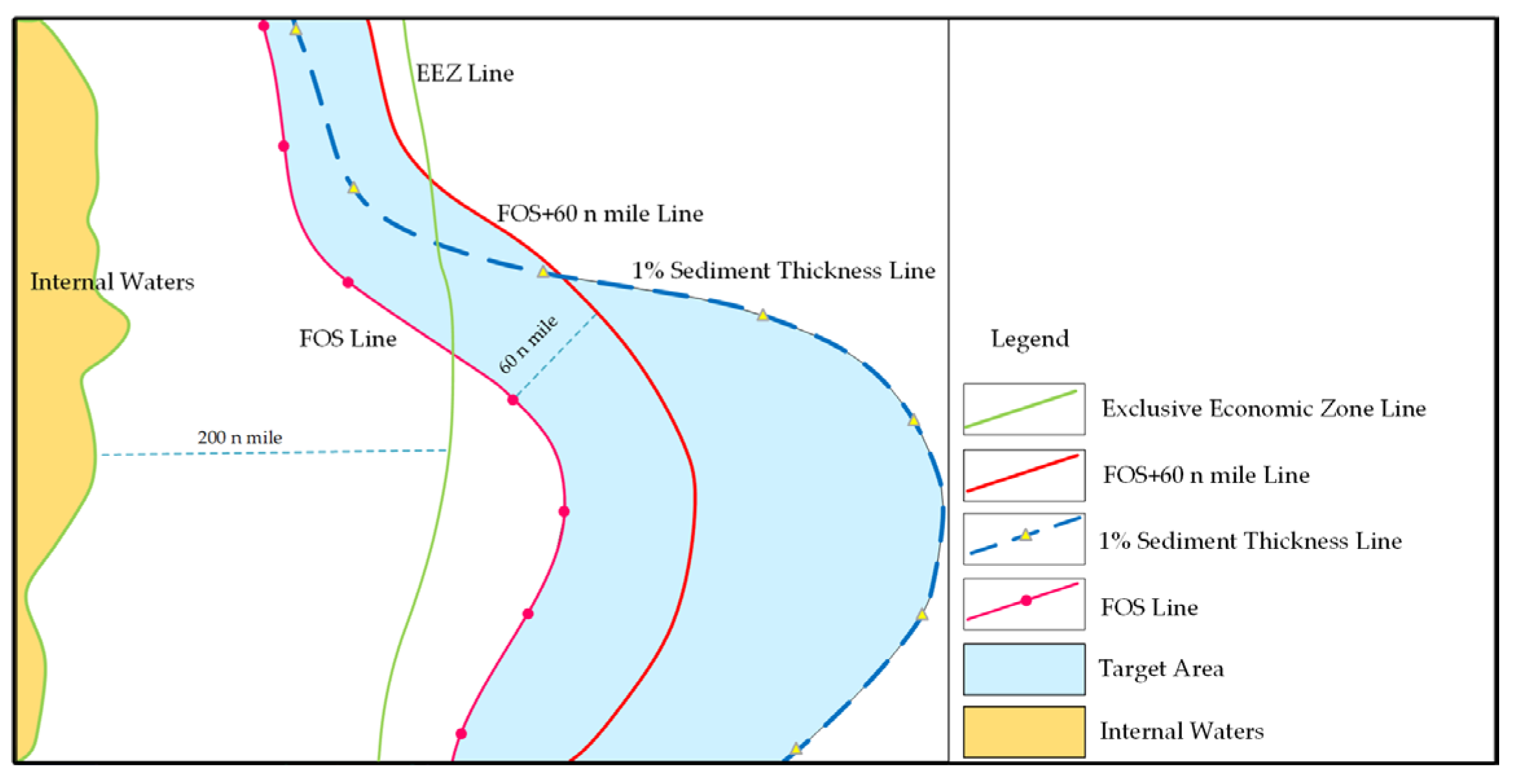
1. Introduction

A maritime delimitation is a national act that determines the scope of maritime sovereignty and rights, directly influencing the maintenance of maritime rights, naval military operations, and coastal defense constructions, thus achieving national strategic objectives. Unlike general maritime delimitation, the determination of the outer limit of the continental shelf relies on seabed topography measurement, marine geological exploration, and geospatial analysis, characterized by strong interdisciplinary connections, high fieldwork difficulty, and precision requirements. The United Nations Convention on the Law of the Sea (hereafter referred to as the Convention) explicitly states: “The coastal State exercises over the continental shelf sovereign rights for the purpose of exploring it and exploiting its natural resources”. The enactment of the Convention has significantly advanced the process by which coastal states scientifically determine the outer limit of the continental shelf, sparking a new round of the “blue land rush” globally [1,2,3,4,5]. Therefore, conducting research on the technologies and methods for delineating the outer limit of the continental shelf holds significant theoretical and practical importance.

The formula limit for the outer limit of the continental shelf (hereafter referred to as formula limit) is the fundamental basis for positively extending boundaries and is jointly determined by the 1% sediment thickness line (the “Irish formula” line) and the foot of the continental slope (FOS)+60 n mile line (the “Hedberg” line). As shown in Figure 1, these two formula lines are closely connected through a compatible disjunctive relationship, and using both lines along with their external envelope line to construct the formula limit can maximize the protection of the coastal state’s legitimate rights. As the starting points for the demarcation by the two formula lines, the convention clearly defines that the foot of the continental slope shall be determined as the point of maximum change in the gradient at its base. regarding the identification of the FOS, there has been relatively mature research. Once the FOS is determined, the process of determining the formula limit can be comprehensively summarized as follows: constructing candidate points sets for the FOS+60 n mile line and the 1% sediment thickness line, systematically selecting points from both candidate sets for the formula limit, and finally generating a delimitation plan.

The candidate points set for the FOS+60 n mile line refer to the collection of fixed points that are no more than sixty nautical miles from the FOS. Its essential meaning is the boundary of the joint buffer zone extended seaward from the FOS in compliance with the constraints of the Convention. The technical core lies in constructing point feature buffer zones starting from the FOS with a radius of sixty nautical miles [6,7]. Scholars from various countries have conducted extensive research on buffer zone construction techniques [8,9,10,11,12,13], Reference [14] introduces a method for generating anisotropic variable distance buffers that conform to the original polygon, unlike the traditional isotropic fixed distance buffers. This method allows for the integrated creation of all buffer boundaries simultaneously. Reference [15] presents an algorithm for generating geometric buffers for vector feature layers and merging these buffers. It starts by constructing a geometric buffer for a vector feature layer, then merges each individual geometric buffer of that layer, and finally merges the overlapping buffers across the entire layer. Reference [16] first proposed the creation of high-precision buffer zones based on the Earth’s ellipsoid and independent of map projections, using geodetic line lengths as the distance measurement standard. This effectively prevents errors in calculating planar buffer zone boundaries due to projection distortions, providing robust technical support for establishing the candidate points set for the FOS+60 n mile line.

Unlike the candidate points set of the FOS+60 n mile line, the determination of the candidate points set of the 1% sediment thickness line requires seismic survey data on sediment thickness for support. Due to spatial continuity constraints, general seismic exploration can only provide information on the vertical distribution of sediments along the survey line, and cannot fully reflect the high-precision sediment thickness distribution across the entire continental rise limit. This results in a highly retrospective evaluation of survey line layout strategies, where decisions must be made between coverage scope and data density during the planning phase. It is difficult to accurately predict which areas require more intensive survey line coverage, and survey line layouts may not maximize the interests of coastal states, leading to a loss of continental shelf area. Therefore, this paper proposes using existing sediment thickness grid data to precisely solve for the distance intervals from the FOS to the sediment grids, quickly selecting potential areas for the 1% sediment thickness line candidate points and constructing the 1% sediment thickness line candidate points set.

According to the principles of topology, the method used to construct polygons from a set of points can lead to variations in the area of the defined spatial region [17]. For any arbitrary polygon, when it is non-convex, the area enclosed is always smaller than that of the smallest convex polygon that can contain it [18]. Therefore, constructing the smallest convex polygon based on a candidate points set can be an effective method for selecting points of the formula limit. Many countries have widely applied and efficient techniques for constructing minimal convex hulls [19,20,21,22,23,24,25,26,27,28]. Building on previous research, reference [18] first proposed applying minimal convex hull construction techniques for selecting baseline points for territorial waters, using the principle of maximizing internal water area to achieve a computer-assisted optimal selection of baseline points. Reference [29] introduced a baseline length threshold-constrained optimization algorithm for selecting territorial sea baseline points, enabling the rapid selection of baseline points under combined constraints of baseline length threshold limit and maximization of internal water areas. This method provides a crucial reference for selecting sets of points for the formula limit with length threshold constraints. This paper uses a unified dataset from both formula lines’ candidate points sets, employing minimal convex hull construction techniques and baseline points optimization algorithm with length threshold limit to construct the set of points of formula limit, thus effectively delineating the formula limit.

2. Materials and Methods

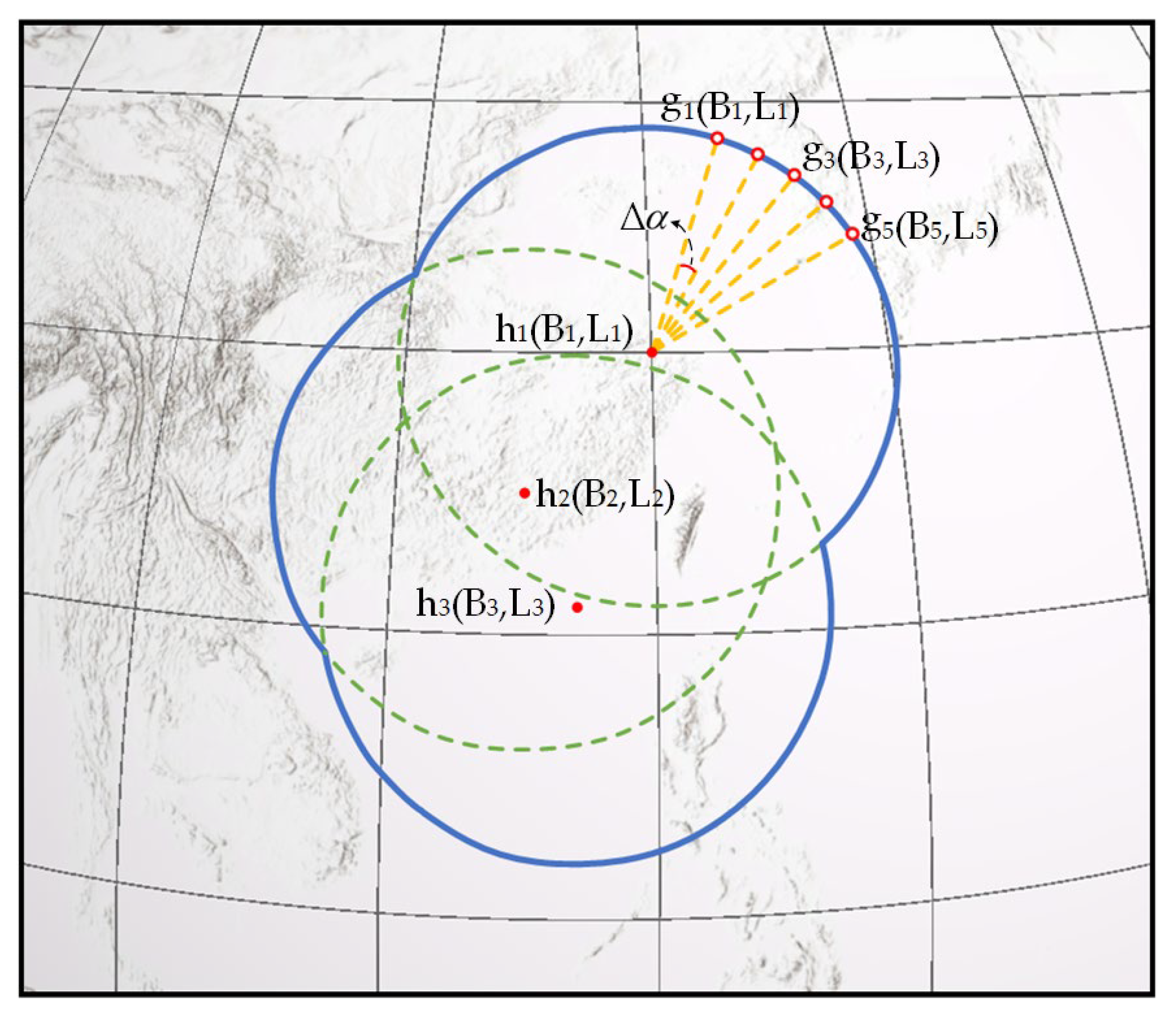
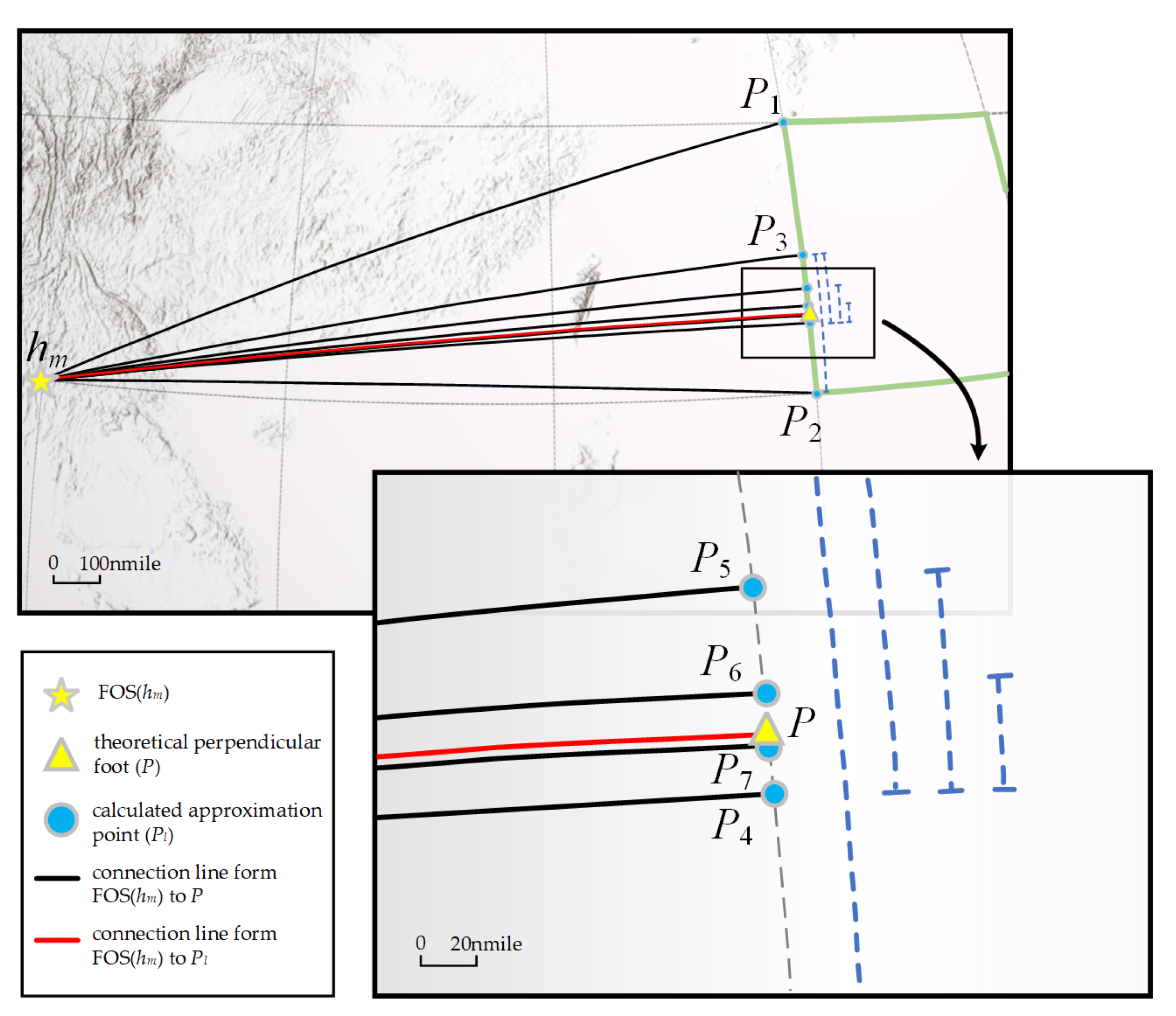
2.1. Calculation of FOS+60 n Mile Line Candidate Points Set

The basic method for constructing a point feature buffer zone on a plane involves using a selected point feature $(x_0,y_0)$ as the center and a buffer distance R as the radius to create a regular circle on the plane. The area enclosed by this circle, denoted $\{(x,y)|\sqrt{{(x-x_0)}^2+{(y-y_0)}^2}\le R\}$, constitutes the desired point feature buffer zone. Due to the transformation relationship between two-dimensional plane coordinates and three-dimensional geographic coordinates, the construction of planar point feature buffer zones is significantly constrained by map projection deformations. With different properties of projections, point feature buffer zones constructed under various projection planes reflect onto the Earth’s sphere with varying degrees of geometric errors. For the same spatial point feature, buffer zones are constructed based on both the Mercator projection plane and the Earth’s ellipsoid with a buffer distance of $R=200 \mathrm{n} \mathrm{mile}$, and the boundaries of the two buffer zones can differ by several kilometers.

To effectively prevent the impact of map projection deformation on buffer zone construction, reference [16] proposed a projection-independent point feature buffer zone construction technique based on the Earth’s ellipsoid, after a thorough analysis of the causes of errors. By using the geodetic line lengths as the distance measure for point feature buffer zones, this method eliminates the boundary displacement errors caused by map projection length deformation, thereby enabling high-precision determination of boundaries for ellipsoidal surface point feature buffer zones. Assuming $(B_0,L_0)$ represents the geographic coordinate of the point feature, and R is the radius of the buffer zone, to construct a buffer zone based on the Earth’s ellipsoidal surface, it is necessary to set an azimuthal increment parameter $\Delta \alpha$. Subsequently, using $(B_0,L_0)$ as the starting point and the buffer radius R as the distance parameter, the azimuth parameter $\alpha$ is selected in equal increments. Utilizing the direct geodetic formula [30], the boundary points $(B_i,L_i)$ are calculated in sequence, thus constructing the collection of boundary points for the point feature buffer zone. The rule for selecting azimuth increments is as follows:

$$\alpha =i\Delta \alpha (i=1,2,3,\dots ,[360/\Delta \alpha ]),$$

(1)

In the Formula (1), $\Delta \alpha$ is the predetermined azimuthal increment parameter. Based on the established buffer radius R, $\Delta \alpha$ has a positive correlation with the distance interval between the buffer zone boundary points; i represents the order of calculation; [] is the rounding symbol. By connecting the calculated points $(B_i,L_i)$ sequentially, the boundary of the point feature buffer zone, precisely expressed in geographic coordinates, can be obtained.

As a coastal state’s FOS consists of multiple point features grouped together, the construction of FOS+60 n mile line in the practice of continental shelf delimitation typically involves the intersection and trimming of multiple point feature buffer zone boundaries. Specifically, the process starts by centering on each element within the coastal state’s FOS set $H=\left\{h_m(B_m,L_m)|m=1,2,\cdot \cdot \cdot ,r\right\}$ (where r is the total number of FOS), and a preliminary candidate points set $G=\{g_n(B_n,L_n)|n=1,2,\dots ,s\}$ (where s is the total number of boundary points of the buffer zones) of FOS+60 n mile line is constructed with a buffer radius of sixty nautical miles. Subsequently, the elements in G are traversed to determine whether they satisfy Equation (2):

$$min\{D_{1n},D_{2n},\dots ,D_{rn}\}<60 (\mathrm{n} \mathrm{mile}),$$

(2)

In the Formula (2), $D_{1n}$, $D_{2n}$, …, $D_{rn}$ represents the geodetic line distance from any element $g_n(B_n,L_n)$ in the candidate set G to each point in the set H. If inequality (2) is satisfied, it indicates that there is at least one point in set H whose distance to element $g_n(B_n,L_n)$ is less than sixty nautical miles. According to Article 76, 4(a)(ii) of the Convention, which defines points on FOS+60 n mile line as being “a line delineated by reference to fixed points not more than 60 nautical miles from the foot of the continental slope” such elements should be excluded from the candidate set. As shown in Figure 2, three solid red points represent the FOS, while the red hollow points are the buffer zone boundary points. After initial exclusion, the elements of candidate set G form a common buffer zone boundary for the FOS, represented by the solid blue line in the figure. Further integration with specific territorial and directional constraints in the delimitation practice allows for the final construction of the candidate points set G of the FOS+60 n mile line on the seaward side within a certain latitude and longitude range.

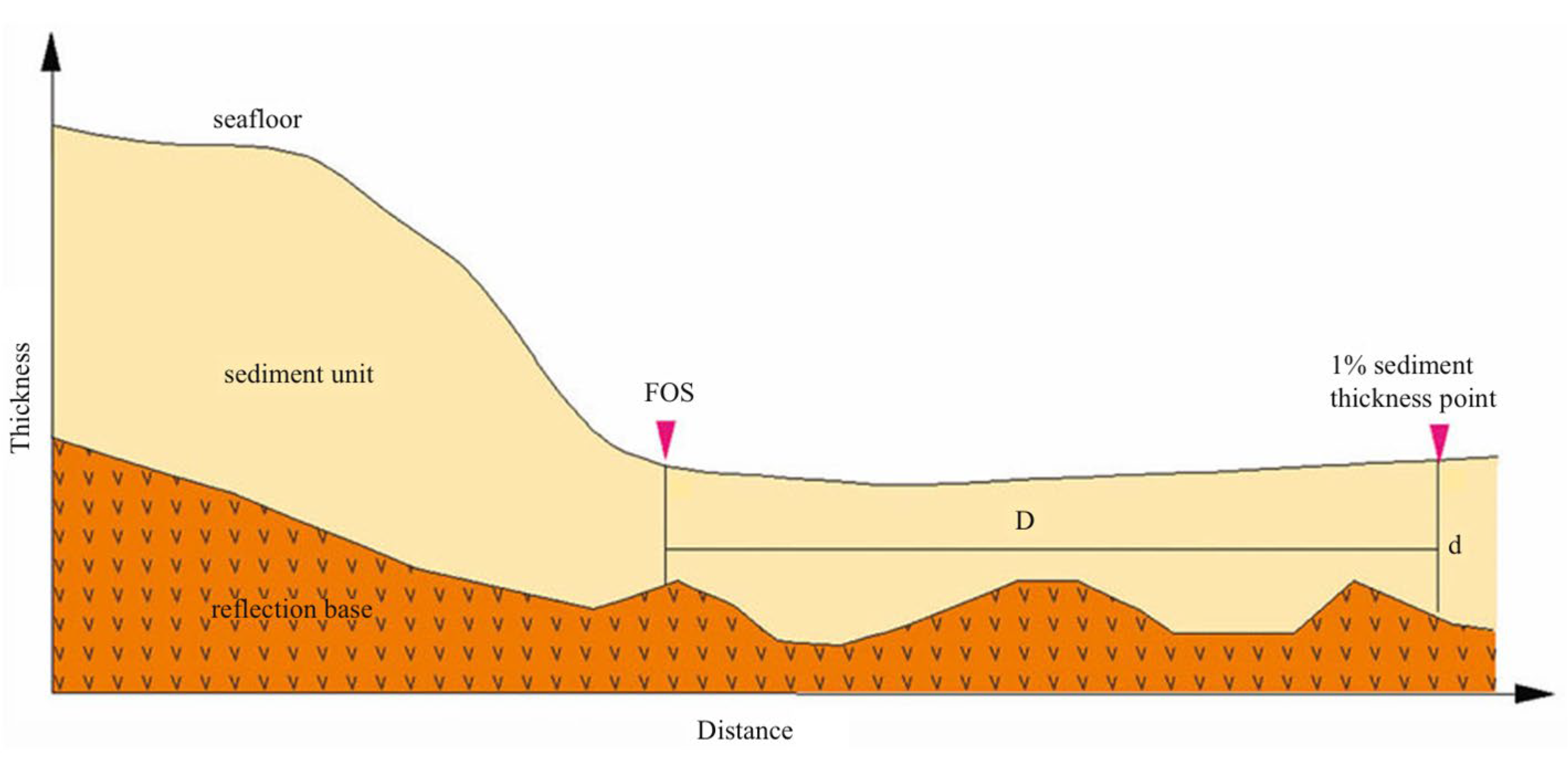
2.2. Calculation of the 1% Sediment Thickness Line Candidate Points Set

In the practice of delimiting the continental shelf, there is no compulsion to use either the FOS+60 n mile line or the 1% sediment thickness line. Coastal states have the right to use the formula that maximizes their national interests and therefore must have the capability to construct both types of formula lines. By comparing them, they can determine which line or combination of both lines encompasses the largest area of the continental shelf. To carry out comprehensive delimitation work, a candidate points set for the 1% sediment thickness line should be established based on the candidate points set of FOS+60 n mile line, and then combine the two under the principle of maximizing the continental shelf area to form the final formula limit. For this purpose, this section uses sediment thickness grid data as the data source, calculating the maximum and minimum distances from the FOS to each grid, by comparing the distance intervals of each grid with the sediment thickness values. This quickly screens potential areas for the 1% sediment thickness line candidate points and determines the usability of each grid in the area. Depending on the usability of the grids, two strategies are adopted to construct the candidate points set for the 1% sediment thickness line. Figure 3 illustrates how to delineate the 1% sediment thickness line. A point can be selected on the 1% sediment thickness line if the sediment thickness d at that point is greater than or equal to the distance D from that point to the FOS.

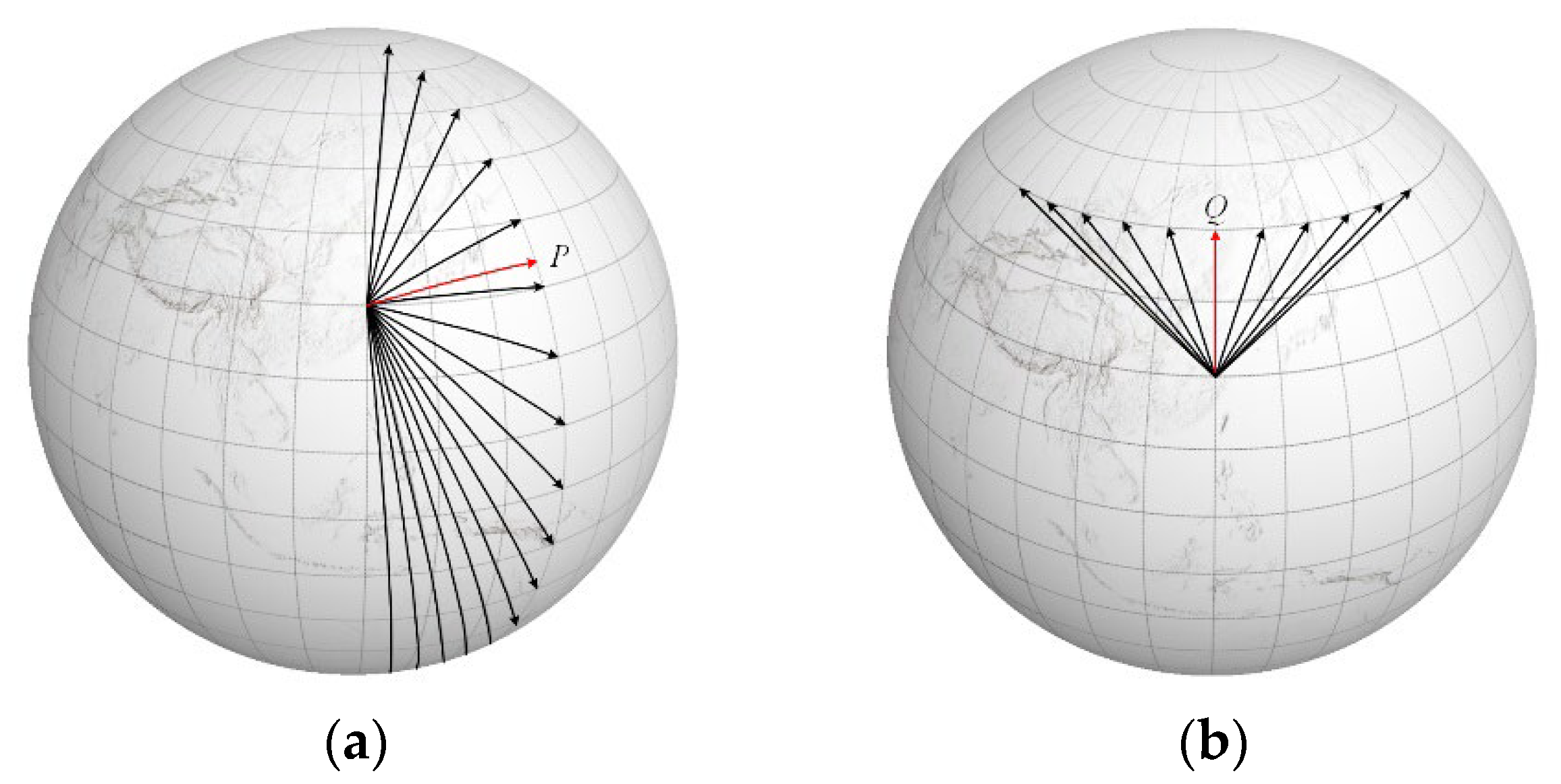
2.2.1. Precision Calculation of Distance Interval

The existing sediment thickness grid data have low resolution, such as the sediment thickness digital database established by the National Genomics Data Center, where the grid resolution is only given in latitude and longitude degrees of $5\min \times 5\min$. Due to the large area covered by a single grid, using it as a unit for delineating the 1% sediment thickness line is not conducive to selecting high-precision candidate points, which ultimately affects the accuracy of the formula line delineation plan. Therefore, this section constructs an ellipsoidal surface grid distance calculation model to compute the maximum and minimum distances from each FOS in the set $H=\left\{h_m(B_m,L_m)|m=1,2,\cdot \cdot \cdot ,r\right\}$ to each sediment grid in collection $W=\{(B_k,L_k,d_k)|k=1,2,\dots ,t\}$ (with $B_k$ and $L_k$ representing the latitude and longitude of the center point of the $k$ grid, $d_k$ for the sediment thickness value, and t for the total number of sediment grids in delimitation area). The distance interval formed by the maximum and minimum distances is defined as the grid distance interval. By assessing the inclusion relationship between the grid distance interval and 100 times the sediment thickness value $(100\times d_k)$, the usability of the grid is determined, thereby quickly screening potential areas for the candidate points of the 1% sediment thickness line.

As shown in Figure 4a, taking the Eastern Hemisphere as an example, when the starting point of the geodetic line is fixed and the longitude difference to the endpoint is determined, the endpoint trajectory forms a meridian. On this meridian, there always exists a specific point P. When this point is the endpoint of the geodetic line, the geodetic line is perpendicular to the meridian at this point. At this time, the geodetic azimuth angle from the endpoint to the starting point is taken as 270° (when the longitude difference from the endpoint to the starting point is positive) or 90° (when the longitude difference is negative), referring to the definition of the shortest distance from a point to a line on an ellipsoidal surface from reference [31]. The geodetic line with point P as the endpoint is the shortest in the cluster of geodetic lines with fixed starting points and determined longitude differences. Furthermore, if the endpoint moves south or north along the meridian from point P, the length of the geodetic line always tends to increase; as shown in Figure 4b, when the starting point of the geodetic line is fixed and the latitude difference to the endpoint is determined, the length of the geodetic line always tends to increase with the increase in the longitude difference from the starting point to the endpoint. When the endpoint Q is on the same meridian as the starting point, this geodetic line is the shortest in the cluster of geodetic lines with a fixed starting point and determined latitude difference.

Referring to the above analysis, the furthest distance from the FOS to a grid bounded by the line of latitude and longitude always exists at the grid corners. The corner coordinates of longitude and latitude can be calculated based on the sediment grid center coordinates and the grid resolution value. Thus, the upper bound of the ellipsoidal grid distance interval, which is the maximum distance from the FOS to the sediment grid, can be defined as:

$$D_{km\max }=\max \{D_{km}{ }^{upper-left},D_{km}{ }^{upper-right},D_{km}{ }^{lower-left},D_{km}{ }^{lower-right}\},$$

(3)

In the Formula (3), $D_{km}{ }^{upper-left}$, $D_{km}{ }^{upper-right}$, $D_{km}{ }^{lower-left}$, $D_{km}{ }^{lower-right}$ represents the geodetic distances from the four corners of a sediment grid $(B_k,L_k,d_k)$ in the set W to an FOS ($h_m$) in the set H, and these distances can be calculated using the reverse solution formula of the geodetic problem [30].

If a specific point P exists on the longitude line boundary of a grid close to the FOS, and the geodetic azimuth angle from this point to the FOS is 90° or 270°, then the geodetic distance from the FOS to this point is the shortest distance to the sediment grid. If this specific point P does not exist on the longitude line boundary of the grid close to the FOS, it indicates that the minimum distance from the FOS to the sediment grid is at the grid corner. To solve for the shortest distance from the FOS to the sediment grid, one must first determine whether the specific point P exists. Taking the Eastern Hemisphere as an example, the rule for determination is as follows:

$$A_{km}{ }^{lower-right}<\frac{\pi }{2}<A_{km}{ }^{upper-right},$$

(4)

$$A_{km}{ }^{upper-left}<\frac{3\pi }{2}<A_{km}{ }^{lower-left},$$

(5)

In Formulas (4) and (5), $A_{km}{ }^{lower-right}$, $A_{km}{ }^{upper-right}$, $A_{km}{ }^{upper-left}$, $A_{km}{ }^{lower-left}$ represent the geodetic azimuth angle from the four corner points of the grid $(B_k,L_k,d_k)$ to a particular FOS ($h_m$). When $h_m$ is located to the east of the grid, the geodetic azimuth angle for the corner points on the right boundary of the grid is calculated, and according to inequality (4), the azimuth angle interval formed by the two corner points is assessed for inclusion of $\frac{\pi }{2}$. If the interval includes $\frac{\pi }{2}$, it indicates that a specific point P certainly exists between the two corner points along the longitude line such that the geodetic line from this point to $h_m$ is perpendicular to the longitude line; similarly, when the $h_m$ is located to the west of the grid, the geodetic azimuth angle for the corner points on the left boundary is calculated, and by inequality (5), it is possible to determine whether a point P exists between the two corner points along the longitude line segment.

Based on the positional relationship between the FOS and the grid, the appropriate judgment rule is selected for assessment. If the determination concludes that the specific point P does not exist, the lower bound of the ellipsoidal grid distance interval, i.e., the shortest distance from the FOS to the sediment grid, can be defined as:

$$D_{km\min }=\min \{D_{km}{ }^{upper-left},D_{km}{ }^{upper-right},D_{km}{ }^{lower-left},D_{km}{ }^{lower-right}\},$$

(6)

If the assessment indicates that the specific point P exists, then the shortest distance from the FOS to the sediment grid should be defined based on the geodetic line distance from point P to the FOS. As shown in Figure 5, on the longitude line boundary (left boundary) of the sediment grid close to the FOS ($h_m$), there exists a point P (depicted as a yellow triangle). The geodetic azimuth angle from this point to the $h_m$ is $\frac{3\pi }{2}$. The coordinates of the two corner points on the left boundary of the sediment grid are designated as $P_1(B_1,L_1)$ and $P_2(B_2,L_1)$, respectively, where $B_1>B_2$.

Referencing the binary search method concept from reference [32], start with the $h_m$ as the starting point and $P_3(\frac{B_1+B_2}{2},L_1)$ as the endpoint. Use the reverse geodetic formula to calculate the geodetic azimuth angle $A_3$ from the endpoint to the starting point and compare it to $\frac{3\pi }{2}$. If $A_3<\frac{3\pi }{2}$, this indicates that the latitude of point P falls within interval $(B_2,\frac{B_1+B_2}{2})$. Continuing with this methodology, use the $h_m$ as the starting point and $P_4(\frac{B_1+3B_2}{4},L_1)$ as the endpoint, calculate the geodetic azimuth angle $A_4$ using the reverse geodetic formula, and assess it against $\frac{3\pi }{2}$. If $A_4>\frac{3\pi }{2}$, this suggests that the latitude of point P falls within interval $(\frac{B_1+3B_2}{4},\frac{B_1+B_2}{2})$. Subsequently, set $P_5(\frac{3B_1+5B_2}{8},L)$ as the endpoint to calculate the geodetic azimuth angle $A_5$. According to the principle of binary search, as the number of calculations increases, the geodetic azimuth angle $A_l$ (where l represents the number of calculations) will converge towards $\frac{3\pi }{2}$, $\underset{l\to \infty }{\lim }{A}_l=\frac{3\pi }{2}$. At this point, the calculated geodetic line distance is defined as the shortest distance $D_{ki\min }$ from the FOS ($h_m$) to the sediment grid.

However, because multiple iterations are not conducive to improving computational efficiency, a tolerance limit $\sigma$ can be manually set according to the delimitation accuracy requirements. Analogous to the triangle inequality in Euclidean space, in ellipsoidal metric space, the difference between any two sides of a triangle is always less than the third side [33], that is, in $\Delta P{P}_l{h}_m$, condition $D_{P_l}{ }_{h_m}>D_{P_l{h}_m}-D_{P{h}_m}$ always holds. Additionally, since $P_l$ and $P_{l-1}$ are, respectively, located on either side of point P, condition $D_{P_l}{ }_{P_{l-1}}>D_{P_l}{ }_{h_m}$ always holds. Therefore, the tolerance limit $\sigma =D_{P_l}{ }_{P_{l-1}}>D_{P_l}{ }_{h_m}>D_{P_l{h}_m}-D_{P{h}_m}$ can be defined such that when the constraint $\sigma$ consistently meets the delimitation accuracy requirements, the geodetic line distance between the FOS ($h_m$) and the specific point P can be replaced by the distance between $h_m$ and $P_l$. With this, the ellipsoidal surface grid distance calculation model is fully constructed.

2.2.2. Selecting Candidate Points from Potential Area

Referencing the constraints of the 1% sediment thickness line, the inclusion relationship between the grid distance interval and 100 times the sediment thickness value is assessed to determine the usability of the grid. For a specific grid within the sediment grid collection $W=\{(B_k,L_k,d_k)|k=1,2,\dots ,t\}$, and for all FOS in the set $H=\left\{h_m(B_m,L_m)|m=1,2,\cdot \cdot \cdot ,r\right\}$, if $100\times d_k<D_{km\min }$ always holds, it indicates that the geodetic line distance from any FOS in the set to any point within the area covered by this sediment grid is greater than 100 times the sediment thickness value. Therefore, the area covered by this grid is not a potential area for the 1% sediment thickness line candidate points, and thus, the usability attribute of this grid should be defined as unavailable. For a specific grid within the collection W, if there exists an FOS ($h_m$) in the set H such that $100\times d_k\ge D_{km\max }$ holds, it implies that the geodetic line distance from all points within the area covered by this sediment grid to the FOS ($h_m$) does not exceed 100 times the sediment thickness value. Therefore, the entire area covered by this grid can be considered a potential area for the 1% sediment thickness line candidate points, and the usability attribute of this grid should be defined as fully available. For a specific grid within the collection W, if there exists an FOS ($h_m$) in the set $H=\left\{h_m(B_m,L_m)|m=1,2,\cdot \cdot \cdot ,r\right\}$ such that $D_{km\min }\le 100\times d_k<D_{km\max }$ holds, it indicates that at least one point within the area covered by this sediment grid has a geodetic line distance to the FOS ($h_m$) that is not greater than 100 times the sediment thickness value at that point. Under the premise that this grid is not fully available, the usability attribute of this grid should be defined as partially available. Additionally, the associated FOS ($h_m$) should be recorded. It is important to note that if there are multiple associated FOSs, all should be recorded.

A grid’s effectively usable range varies depending on the grid’s usability status. For three grids with the same area but different usability statuses, the fully available grid has a larger effectively usable range than the partially available grid, which in turn is larger than the unavailable grid. Theoretically, all points within the area covered by a fully available grid can be used as candidate points for the 1% sediment thickness line. However, from a practical application perspective, the four corners of a sediment grid effectively define the scope of the grid area, and their lower data volume helps optimize computational efficiency. Therefore, for fully available grids, their corner points should be used as candidate points and added to the 1% sediment thickness line candidate points set. The key to utilizing partially available grids lies in how to segregate the usable and non-usable parts according to the requirements of the Convention. As described in Section 2.2.1, in the process of determining a grid as partially available, its associated FOS ($h_m$) is also recorded. Referring to ellipsoidal point feature buffer zone construction techniques, using $h_m$ as the center and 100 times the sediment thickness value $(100\times d_k)$ as the buffer radius, a set of buffer zone boundary points is constructed. Subsequently, the intersection of this point set with the area covered by the grid is calculated to identify the point features, which should then be added to the 1% sediment thickness line candidate points set. It is important to note that, to improve computational efficiency during the buffer zone construction process using the associated FOS ($h_m$) as the point feature, the azimuth angle $\alpha$ selection rule can be redefined based on Formula (1) as follows:

$$\alpha ={\alpha }_{\min }+i\Delta \alpha (i=1,2,3,\dots ,[({\alpha }_{\max }-{\alpha }_{\min })/\Delta \alpha ]),$$

(7)

In Formula (7), ${\alpha }_{\min }$ and ${\alpha }_{\max }$ represent the minimum and maximum geodetic azimuth angles from the associated FOS ($h_m$) to the four corners of the grid. By limiting the range of the azimuth angle $\alpha$, a large number of irrelevant buffer zone boundary points can be eliminated, enhancing the efficiency of constructing the 1% sediment thickness line candidate points set. With this, for grids of different usability, this study employs two differentiated selection strategies to achieve the complete construction of the 1% sediment thickness line candidate points set.

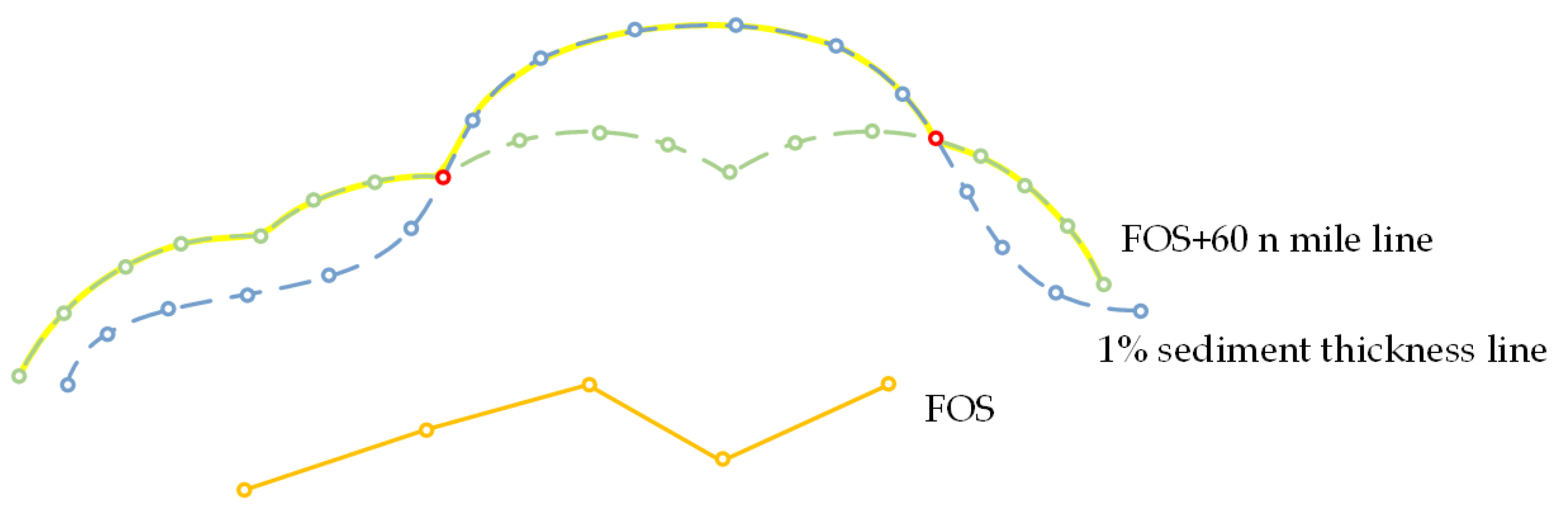
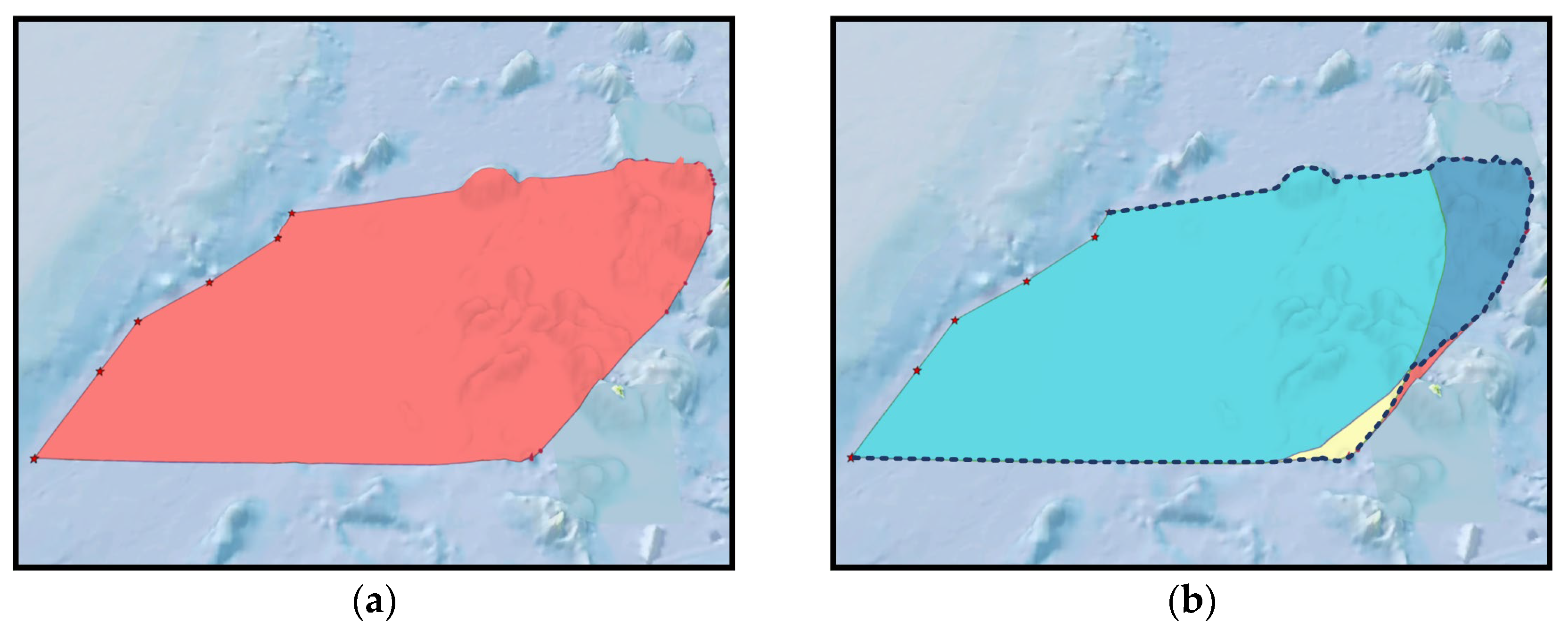
2.3. Constructing Formula Limit Based on Two Candidate Points Sets

The FOS+60 n mile line and the 1% sediment thickness line are two boundaries drawn according to different rules, both of which can independently serve as the outer boundary of the continental shelf and are recognized by the Convention. However, when the two lines intersect, to ensure the maximization of coastal state interests, it is necessary to consider using both as the basis for delineating the formula limit of the continental shelf. How to handle the topological relationship between the two is the key to planning a comprehensive delineation scheme. According to reference [34], it is suggested that the intersection points of the two formula lines should be determined first, and then the outer segments of the two formula lines towards the sea should be selected based on these intersection points and combined to form a coherent external envelope line. As shown in Figure 6, the green dashed line represents the FOS+60 n mile line, and the blue dashed line represents the 1% sediment thickness line. To calculate the external envelope line of the two formula lines, the intersection points of the two formula lines need to be determined first. Then, based on these intersection points, the outer segments of the two formula lines towards the sea are selected and combined to ultimately achieve the construction of the external envelope line (shown as the yellow solid line in the figure). Although this method can delineate the formula limit of the continental shelf while complying with the Convention, there are still two limitations. Firstly, the calculation process requires solving the technical problem of accurately intersecting two geodesic lines on the ellipsoidal surface. Secondly, due to the failure to fully utilize geometric construction rules, delineating the outer formula limit of the continental shelf in this way may result in partial loss of the continental shelf area of the coastal state.

The “fixed points” described in Article 76, paragraphs 4, 5, and 7 of the Convention should be clearly defined as specific latitude and longitude coordinates determined according to the method described in Article 4(a) of the Convention. Drawing on the approach outlined in reference [18] for the optimal selection of baseline points using the convex hull construction technique, this paper integrates the construction of the formula limit by combining two sets of formula line candidate points. While strictly adhering to the Convention’s definition of “fixed points” to delineate the formula limit, the paper maximizes the extension of the continental shelf area to ensure the maximization of coastal state interests. As shown in Figure 7, when generating the outer envelope line of the two formula lines, the focus is no longer solely on individual formula lines but on merging the candidate points of the FOS+60 n mile line with those of the 1% sediment thickness line, treating them uniformly as the dataset for constructing the convex hull. The yellow solid line in the figure represents the outer envelope line of the two formula lines derived from the convex hull construction technique, while the gray area illustrates the difference in area between the continental shelf region constructed based on the maximum area principle and that determined by the traditional intersection method. It is important to note that, when constructing the minimum convex polygon, the former pays special attention to the length limitation requirement for the geodesic distances between adjacent boundary points stipulated in the Convention. For line segments exceeding sixty nautical miles, an adjustment is made using a baseline points optimization algorithm based on length threshold limitation. This ensures that the boundary scheme constructed by this method not only complies with the Convention’s restrictions but also undergoes precise optimization based on the principle of maximizing the continental shelf area. Following the specifications of the Convention, this method avoids complex calculations of geodesic line intersections on the ellipsoidal surface, effectively achieving coastal state gains in the delineation of the continental shelf.

3. Experiments and Numerical Analysis

To validate the effectiveness of the algorithm, this paper implements the construction of candidate point sets for the FOS+60 n mile line, 1% sediment thickness line, and the formula limit for a specific sea area through programming in Visual Studio 2022. It also generates the corresponding delimitation plan. The delimitation results are visualized, and the area calculations are performed using ArcGIS Pro (Esri, Redlands, CA, USA), with the experiments conducted using the geocentric coordinate system WGS-1984. The experimental setup utilizes an Intel(R) Core(TM) i7 processor with a clock speed of 2.6 GHz and 16 GB of RAM. The sediment thickness data used in the experiments are sourced from the sediment thickness digital database of the National Genomics Data Center, with the geographical grid resolution being $5 \min \times 5 \min$.

The FOS set $H=\left\{h_m(B_m,L_m)|m=1,2,\cdot \cdot \cdot ,6\right\}$ was sourced from the digital executive summary data of a national delimitation case published by the United Nations Commission on the Limits of the Continental Shelf. Under conditions of a specified latitude range, using six FOS as a point group and a sixty nautical mile radius for the buffer zone, the candidate points set for the FOS+60 n mile line constructed using ellipsoidal surface point group buffer zone technology are shown in Figure 8a. The red five-pointed stars represent the coastal state’s FOS, and the blue dots indicate the candidate points for the FOS+60 n mile line. The potential areas for the candidate points of the 1% sediment thickness line were filtered using the ellipsoidal surface grid distance calculation model and constructed using two different selection strategies, as shown in Figure 8b. The mapping results within the same geographical framework are presented in Figure 8c.

Combining

Table 1. Geodetic line distances between adjacent points on the formula lines.

Serial Number (Start–End Points)	FOS+60 n Mile Line (m)	1% Sediment Thickness Line (m)
1–2	9256.8	15,845.6
2–3	9256.8	5558.3
3–4	9256.8	1978.3
4–5	9256.8	1978.3
5–6	9256.8	1978.3
6–7	9256.8	21,183.1
7–8	9256.8	20,443.3
8–9	2101.0	12,322.3
9–10	9256.8	12,839.9
10–11	9256.8	13,193.1
11–12	9256.8	15,669.7
12–13	9256.8	12,795.9
13–14	9256.8	17,752.7
14–15	4629.4	11,829.1
15–16	--	3490.4

, the geodetic line distances between adjacent points on the two formula lines demonstrate that by judiciously selecting azimuthal increment parameters and utilizing baseline points optimization algorithm constrained by length threshold, the boundary points of both formula lines can meet the requirements set by Article 76 of the Convention, which mandates that the line connecting boundary points not exceed a length threshold of sixty nautical miles. As shown in Figure 8c, based on the same set of FOS, the FOS+60 n mile line and the 1% sediment thickness line intersect, leading to a significant overlap between the continental shelf areas delineated independently by the two formula lines. Referring to

Table 2. Area comparison of continental shelf regions constructed based on a single formula line and the union of two formula lines (intersection method).

	FOS+60 n Mile Line	1% Sediment Thickness Line	Combined Region
Area (m2)	13,501,729,047	14,995,785,392	15,218,132,884

, although the continental shelf area delineated by the 1% sediment thickness line is larger, with a difference of 1,494,056,345 m² compared to the FOS+60 n mile line, it is still less than the total area of the continental shelf regions combined (i.e., the intersection method continental shelf area), which shows an area gain of 222,347,492 m² when compared to the 1% sediment thickness line area.

Using the combined candidate point sets of the FOS+60 n mile line and the 1% sediment thickness line as the basic data source, the minimal convex hull construction technique and the baseline points optimization algorithm constrained by length threshold are applied sequentially to eliminate redundant candidate points from both sets. The result, illustrating the formula limit area, is shown in Figure 9a, where the FOS are marked with red five-pointed stars, and the formula limit points set is indicated by red dots. The geographic framework displaying the continental shelf area constructed based on the principle of maximum area, alongside the traditional intersection method, is depicted in Figure 9b. In the diagram, the blue dashed line encircles the area adjacent to the FOS, representing the combined continental shelf areas of the FOS+60 n mile line and the 1% sediment thickness line, i.e., the area constructed using the intersection method.

As shown in

Table 3. Geodetic line distances between adjacent points on the formula limit according to the maximum area principle.

Serial Number (Start–End Points)	Geodetic Line Distances (m)
1–2	15,845.6
2–3	5558.3
3–4	1978.3
4–5	1978.3
5–6	1978.3
6–7	21,183.1
7–8	20,443.3
8–9	12,322.3
9–10	65,318.7
10–11	4629.4

, the geodetic line distances between adjacent points of the formula limit constructed based on the principle of maximum area do not exceed the sixty nautical mile length threshold stipulated by Article 76, paragraph 7 of the Convention. Utilizing the candidate point sets of the FOS+60 n mile line and the 1% sediment thickness line as data sources to build the minimal convex hull, compared to directly deriving the combined areas of the two formula lines, the area gain for the formula limit area constructed under the maximum area principle can reach 77,278,427 m². Figure 9 and

Table 4. Area comparison of continental shelf constructed based on the intersection method and the maximum area principle.

	Intersection Method	Maximum Area Principle
Area (m2)	15,218,132,884	15,295,411,311

respectively illustrate the area gain of the continental shelf region constructed under the maximum area principle compared to the traditional intersection method, from both graphical and numerical perspectives.

4. Conclusions

As a key region rich in marine resources, the continental shelf holds profound strategic importance for coastal states. Precise delimitation of the continental shelf not only concerns the effective utilization of resources and the protection of maritime rights but also supports the maintenance of national maritime sovereignty and promotes cooperation in regional maritime management. This paper, based on the descriptions in the United Nations Convention on the Law of the Sea of the “fixed point” along the formula limit of the continental shelf, thoroughly justifies the rationale for delineation work using dual candidate point sets. From the perspective of maximizing the protection of coastal states’ legal rights, it constructs a complete technical process for delineating the formula limit of the continental shelf, providing an effective reference for countries to conduct such delimitation. Experimental data of Table 1 and Table 2 indicate that by judiciously selecting azimuthal increment parameters and utilizing baseline points optimization algorithm constrained by length threshold, both the FOS+60 n mile line and the 1% sediment thickness line can meet the 60 nautical mile length constraint of the Convention. However, the area of the continental shelf delineated by relying on a single formula line is always smaller than the area of the continental shelf delineated by relying on the intersection method. The experimental data of Table 3 and Table 4 indicate that the formula limit constructed based on the maximum area principle, under the condition of meeting the 60 nautical mile length constraint of the Convention, can effectively increase the continental shelf area of the coastal state compared to the traditional intersection method.

It is important to note that in a comprehensive delimitation plan, the scope of the continental shelf area is not only constrained by the formula limit but also by the depth constraint line (2500 m + 100 n mile) and the distance constraint line (350 n miles), which are closely linked through a compatible disjunctive relationship, jointly limiting the maximum extension of the coastal state’s continental shelf boundary. Therefore, in practical delimitation operations, it is essential to consider the topological relationship between the formula limit and the restrictive limit. The next steps involve integrating the ellipsoidal line element buffer zone construction technique and the seabed geomorphological characterization method to continue research based on Convention two counteracting rules to build external restrictive limits, thereby forming a complete set of continental shelf delimitation techniques.

References

- Sun, Q.; Fang, Y.; Li, J. Science and technology of delimitation of continental shelf and its application in Maritime Silk Road cooperation. Adv. Earth Sci. 2018, 33, 1215–1222. [Google Scholar]
- Fang, Y.; Yin, J. Progress of Work in the Commission on the Limits of the Continental Shelf and Hot Issues on the Extended Continental Shelf Delineation Worldwide. Chin. Rev. Int. Law 2020, 7, 61–69. [Google Scholar]
- Fang, Y.; Li, J.; Li, M.; Tang, Y.; Yin, J. Principles and methods for the submission consideration of the Commission on the Limits of Continental Shelf-Cases study of recommendations summary made by the Commission. J. Mar. Sci. 2013, 31, 1–9. [Google Scholar]
- Fang, Y.; Li, J.; Yin, J.; Liu, W.; Tang, Y. Principles and methods for determining the foot of the continental slope. J. Mar. Sci. 2022, 40, 1–9. [Google Scholar]
- Liu, Z.; Liu, J.; Jin, J. Study to Automatic Drawing of Foot Line of Extended Continental Slope. Comput. Eng. Appl. 2007, 43, 240–241. [Google Scholar]
- Wu, Z.; Yang, F.; Tang, Y. High-Resolution Seafloor Survey and Applications; Springer: Singapore, 2021. [Google Scholar] [CrossRef]
- Wu, Z.; Li, J.; Jin, X.; Fang, Y.; Shang, J.; Li, S. Methods and Procedures to Determine the Outer Limits of the Continental Shelf beyond 200 Nautical Miles. Acta Oceanol. Sin. 2013, 32, 126–132. [Google Scholar] [CrossRef]
- Wang, J.; Yu, Q.; Chen, Y. A Novel Method of Buffer Generation Based on Vector Boundary Tracing. In 2009 International Forum on Information Technology and Applications; IEEE: Chengdu, China, 2009; Volume 1, pp. 579–582. [Google Scholar] [CrossRef]
- Dong, P.; Yang, C.; Rui, X.; Zhang, L.; Cheng, Q. An Effective Buffer Generation Method in GIS. In 2003 IEEE International Geoscience and Remote Sensing Symposium—IGARSS, Proceedings of the IEEE International Symposium on Geoscience and Remote Sensing (IGARSS), Toulouse, France, 21–25 July 2003; IEEE: New York, NY, USA, 2003; pp. 3706–3708. [Google Scholar]
- Bader, M.; Weibel, R. Detecting and Resolving Size and Proximity Conflicts in the Generalization of Polygonal Maps. In Proceedings of the 18th International Cartographic Conference, Stockholm, Sweden, 23–27 June 1997; pp. 23–27. [Google Scholar]
- Wu, H. Problem of Buffer Zone Construction in GIS. Geomat. Inf. Sci. Wuhan Univ. 1997, 22, 57–65. [Google Scholar]
- Bolstad, P. GIS Fundamentals: A First Text on Geographic Information Systems, 6th ed.; XanEdu: Ann Arbor, MI, USA, 2019. [Google Scholar]
- Žalik, B.; Zadravec, M.; Clapworthy, G.J. Construction of a Non-Symmetric Geometric Buffer from a Set of Line Segments. Comput. Geosci. 2003, 29, 53–63. [Google Scholar] [CrossRef]
- Mu, L. A Shape-Based Buffering Method. Environ. Plan. B-Plan. Des. 2008, 35, 399–412. [Google Scholar] [CrossRef]
- Bhatia, S.; Vira, V.; Choksi, D.; Venkatachalam, P. An Algorithm for Generating Geometric Buffers for Vector Feature Layers. Geo-Spat. Inf. Sci. 2013, 16, 130–138. [Google Scholar] [CrossRef]
- Peng, R.; Wang, J. A Research on Creating Buffer on the Earth Ellipsoid. Acta Geod. Cartogr. Sin. 2002, 31, 270–273. [Google Scholar]
- Munkres, J.R. Topology; Pearson: New York, NY, USA, 2018. [Google Scholar]
- Peng, R.; Wang, J.; Tian, Z.; Guo, L.; Chen, Z. A Research for Selecting Baseline Point of the Territorial Sea Based on Technique of the Convex Hull Construction. Acta Geod. Cartogr. Sin. 2005, 34, 53–57. [Google Scholar]
- Wang, J. Study of Optimizing Method for Algorithm of Minimum Convex Closure Building for 2D Spatial Data. Acta Geod. Cartogr. Sin. 2002, 32, 82–86. [Google Scholar]
- Jin, W.; He, T.; Liu, X.; Tang, W.; Tang, R. A Fast Convex Hull Algorithm of Planar Point Set Based On Sorted Simple Polygon. Chin. J. Comput. 1998, 21, 533–539. [Google Scholar]
- Guo, R. Spacial Analysis; Wuhan Techinical University of Surveying and Mapping Press: Wuhan, China, 2000. [Google Scholar]
- Liu, R.; Yang, D.; Li, Y.; Chen, K. An Improved Algorithm for Producing Minimum Convex Hull. J. Geod. Geodyn. 2011, 31, 130–133. [Google Scholar] [CrossRef]
- Preparata, F.P.; Shamos, M.I. Computational Geometry: An Introduction; Springer-Verlag: New York, NY, USA, 2012. [Google Scholar]
- Brönnimann, H.; Iacono, J.; Katajainen, J.; Morin, P.; Morrison, J.; Toussaint, G. Space-Efficient Planar Convex Hull Algorithms. Theor. Comput. Sci. 2004, 321, 25–40. [Google Scholar] [CrossRef]
- Gamby, A.N.; Katajainen, J. Convex-Hull Algorithms: Implementation, Testing, and Experimentation. Algorithms 2018, 11, 195. [Google Scholar] [CrossRef]
- Avis, D.; Bremner, D.; Seidel, R. How Good Are Convex Hull Algorithms? Comput. Geom.-Theory Appl. 1997, 7, 265–301. [Google Scholar] [CrossRef]
- Barber, C.B.; Dobkin, D.P.; Huhdanpaa, H. The Quickhull Algorithm for Convex Hulls. ACM Trans. Math. Softw. 1996, 22, 469–483. [Google Scholar] [CrossRef]
- Kirkpatrick, D.G.; Seidel, R. The Ultimate Planar Convex Hull Algorithm? SIAM J. Comput. 1986, 15, 287–299. [Google Scholar] [CrossRef]
- Dong, J.; Peng, R.; Li, N.; Liu, G.; Tang, L. Optimal Selection Algorithm of Territorial Sea Baseline Points with the Limitation of Baseline Length Threshold. Geomat. Inf. Sci. Wuhan Univ. 2023, 48, 1473–1481. [Google Scholar] [CrossRef]
- Xiong, J. Ellipsoidal Geodesy; People’s Liberation Army of China Press: Beijing, China, 1988. [Google Scholar]
- Zhang, J.; Jin, J. Marine delimitation method based on earth ellipsoid model. Sci. Surv. Mapp. 2013, 38, 16–17+30. [Google Scholar] [CrossRef]
- Qu, W. Algorithm Design and Analysis, 3rd ed.; Tsinghua University Press: Beijing, China, 2023. [Google Scholar]
- Gallot, S.; Hulin, D.; Lafontaine, J. Riemannian Geometry; Springer: Berlin, Germany, 2004. [Google Scholar]
- International Hydrographic Organization. A Manual on Technical Aspects of the United Nations Convention on the Law of the Sea, 1982, 6th ed.; Ocean Press: Beijing, China, 2021. [Google Scholar]