Fully Coupled Hydrodynamic–Mooring–Motion Response Model for Semi-Submersible Tidal Stream Turbine Based on Actuation Line Method

Abstract

The modeling of floating tidal stream energy turbine (FTSET) systems demands significant computational resources, especially when incorporating fully coupled models that integrate hydrodynamics, mooring, motion response, and their interactions. In this study, a novel hybrid numerical model for FTSET systems has been developed, utilizing the open-source software OpenFOAM. The hydrodynamic characteristics of three-bladed vertical-axis turbines are simulated in steady, three-dimensional wave–current numerical tanks using an unsteady actuator line method (UALM). The interFoam two-phase Navier–Stokes solver within OpenFOAM is utilized to manage the kinematic characteristics of the floating platform. Mooring dynamics are addressed using the mass–spring–damper model (MoorDyn), and turbine wake dynamics are resolved using a buoyancy-modified RANS turbulence model. The comprehensive model can simulate wave, flow, mooring dynamics, platform motion, and the interactions between the turbine and platform within FTSET systems. To validate the model, several scenarios are analyzed, and experiments are conducted to validate the numerical results. The model accurately predicts platform motion responses and mooring line tensions, especially under wave–current conditions, capturing the interconnected effects of platform motion during turbine rotation. Additionally, the model extends predictions of turbine–platform wake development and interaction.

1. Introduction

The ocean presents substantial potential for renewable energy, which is crucial for global energy transformation, climate change mitigation, and pollution control [1]. Tidal stream energy, a significant component of marine renewable energy, boasts unique advantages such as high predictability, high energy density, good load stability, and large reserves compared to other forms of ocean energy like wave energy [2]. Fixed turbines have limited utility in deeper waters, whereas deep-sea areas offer more abundant space and tidal resources. Floating turbines provide a solution for harnessing deep-sea tidal stream energy [3,4]. Furthermore, the structural and operational similarities between tidal and wind power technologies facilitate the rapid advancement of tidal stream energy towards industrial maturity [5]. The adoption of floating platforms makes turbine systems easier to install and maintain, adaptable to various water depths, and less dependent on seabed topography. Furthermore, turbines can capture more energy due to the higher flow velocities near the water surface [6,7]. Studying multi-energy complementary systems has become mainstream, making the integration of tidal stream turbines into floating multi-energy systems crucial [8]. This integration improves power generation efficiency and mitigates challenges related to floating structures, including installation and maintenance costs.

The current focus of marine renewable energy research has shifted towards deep-sea projects [9], which must consider the increasing influence of waves [10]. The dynamics of floating tidal stream energy turbine (FTSET) systems require consideration of the interactions among the floating platform, tidal stream turbine, and mooring system [11]. Floating structures exhibit dynamic characteristics governed by more complex physical principles than fixed structures. The loads induced by waves result in six degrees of freedom of motion on the platform, affecting the turbine dynamics, force distribution, variations in cable tension, and wake fields. Moreover, tidal turbines undergo significant energy extraction and thrust oscillations due to wave–current interactions, leading to intense dynamic loads. These fluctuations in power and force reciprocally affect the floating platform. For example, tidal currents alter the platform’s initial position and orientation, intensifying the amplitude of the platform’s motion response and changing mooring tension distribution [12]. Previous studies [13] have made progress in modeling various components of the FTSET system, such as turbine performance in wave and current environments and the dynamic properties of the mooring line. However, the FTSET model should incorporate all coupled physical factors and accurately describe the interactions between hydrodynamics, mooring, and kinematic responses.

Recent advancements in numerical simulation research have significantly improved our understanding and provided solutions for modeling floating turbines [14,15,16,17,18,19,20]. For example, Ma et al. [15] successfully simulated turbine performance under rotational and surge motions in combined wave and current environments using moving and sliding mesh techniques. Their study showed that dual-rotor turbines can increase average power output by up to 15.3% compared to single rotors across various wave frequencies, amplitudes, and tip speed ratios. Similarly, Brown et al. [14] developed a generalized coupling model to evaluate floating tidal stream turbines [21,22], emphasizing the importance of considering the operational characteristics of anchors, turbines, and platforms in coupled analyses and noting differences in load between floating and fixed systems. Wang et al. [17] explored the hydrodynamic performance of horizontal-axis tidal energy turbines on floating platforms under wave–current conditions using CFD methods and proposed a rapid prediction method for assessing hydrodynamic loads under complex conditions [19]. Zhang et al. [13,20] quantified the wake effects and motion responses of tidal energy turbines under single-degree-of-freedom motion. This type of numerical simulation typically relies on a forced oscillation approach to study the variation in wave parameters, potentially neglecting fundamental wave–current interactions.. Additionally, the high-fidelity methods requiring tens of millions of grids significantly increase computational costs and can hinder further exploration in the engineering field.

Modeling floating tidal stream energy turbine (FTSET) systems using high-fidelity approaches involve significant computational challenges, particularly when fully coupled models are required to integrate hydrodynamics, moorings, kinematic responses, and their interactions. To enhance computational efficiency while maintaining accuracy, Bachant et al. [23] initially developed the Actuator Line Model (ALM) library for vertical-axis wind turbines. They validated it with experimental measurements and blade-resolved simulations. This method improves efficiency by eliminating boundary layer grids on the blade surface and employing sliding or overset grid techniques during blade rotation. Additionally, turbinesFoam integrates source terms within the fvOptions framework, ensuring compatibility with various solvers and turbulence models, making it suitable for multiphase simulations, including those using the interFoam solver. Fleming et al. [24] applied this method to study the impact of upstream turbine yaw, tilt, and positioning on downstream turbines. Stanly et al. [25] introduced a new tip-correction-based filtered ALM that accommodates coarser-than-optimal grids without overpredicting thrust. Deng et al. [26] used ALM-IBM to construct a model incorporating low computing resources to analyze the scour pattern of hydraulic turbines. Furthermore, Cheng et al. [27] and Yu et al. [28] employed the unsteady ALM (UALM) to analyze the coupled aerodynamics of semi-submersible or truss-type floating offshore wind turbines, highlighting the ALM’s effectiveness in simulating turbine blades.

To address the challenges of wave–current interactions, mooring dynamics, and the coupled responses of floating platforms and turbines while conserving computational resources, this study employs OpenFOAM to develop a model capable of nonlinearly interacting with the platform under the combined effects of waves and currents. The model also accounts for the structural dynamics of blade rotations and mooring lines. This improved model, regular wave generation, and uniform water flow are simulated using the olaFlow solver. Hydrodynamic issues of the turbine are addressed with an upgraded unsteady actuator line method (UALM) solver. Mooring dynamics are integrated using the lumped-mass mooring code, MoorDyn, as detailed by Hall and Goupee [29]. By combining olaFlow, UALM, and MoorDyn, this model, referred to as FOAM-FT, accurately and efficiently simulates the entire FTSET system. The effectiveness of the FOAM-FT simulation structure will be confirmed through physical model experiments. The turbine’s performance, platform motion response, and mooring tension loads are validated using experimental results from other studies [12]. Additionally, the formation and interaction of turbine wakes will be thoroughly explored. The manuscript is structured as follows: Section 2 describes the numerical methods, Section 3 outlines the design and validation of the physical model, Section 4 analyzes the wake of turbines under floating conditions and their integration with platform wake fields, and Section 5 presents the conclusions.

2. Methodology

This study utilized the open-source computational fluid dynamics (CFD) toolbox OpenFOAM for CFD modeling and employed the olaFlow toolbox to develop a three-dimensional numerical wave–current tank. The enhanced unsteady actuator line method (UALM) model was used to simulate the turbine, while MoorDyn V2 was employed for mooring dynamics modeling. The motion of the floating body was efficiently simulated by solving the Reynolds-averaged Navier–Stokes (RANS) equations within the CFD flow solver. This section details the essential components of the coupled CFD-mooring model.

2.1. Numerical Fluid Dynamics Methodology

The two-phase flow solver, interFoam, implemented within the OpenFOAM framework (OpenFOAMv2012) and based on the Reynolds-averaged Navier–Stokes (RANS) equations, is widely used in fluid dynamics research. This study employs the olaFlow toolbox (https://github.com/phicau/olaFlow, accessed on 16 May 2024) to develop a three-dimensional numerical wave–current tank. The olaFlow model allows for the generation and absorption of water waves and their interactions with coastal structures. OlaFlow represents an evolution from its predecessors, IH-FOAM and OLAFOAM [30]. The computational domain of the model is illustrated in Figure 1.

The wave field is governed by the continuity equation, the RANS equations, and the Volume of Fluid (VOF) equation [31]:

$${\displaystyle \mathsf{\nabla }}·u=0$$

(1)

$$\frac{\mathsf{\partial }\rho u}{\mathsf{\partial }t}+\mathsf{\nabla }\cdot (\rho uu)-\mathsf{\nabla }\cdot ((\mu +{\mu }_{tur})\mathsf{\nabla }u)=C\kappa \mathsf{\nabla }\alpha -gX\mathsf{\nabla }\rho -\mathsf{\nabla }{P}_{\rho gh}$$

(2)

$$\frac{\mathsf{\partial }\alpha }{\mathsf{\partial }t}+\mathsf{\nabla }\cdot (\alpha u)+\mathsf{\nabla }\cdot [\alpha \left(1-\alpha \right)U_r]=0$$

(3)

where $u$ is the velocity vector; $\alpha$ is the volume fraction of fluid in each cell, i.e., 0 for air and 1 for water, with values between 0 and 1 indicating cells containing a mixture of the two fluids; ${\mu }_{tur}$ is the dynamic turbulent viscosity; $C\kappa \mathsf{\nabla }\alpha$ is the surface tension term, where $C$ is the surface tension coefficient, and $\kappa$ is the interface curvature. $g$ is the gravitational acceleration; and $\rho$ and $\mu$ are the weighted density and dynamic viscosity of two phases, respectively, calculated as follows:

$$\rho =\alpha {\rho }_1+\left(1-\alpha \right){\rho }_2$$

(4)

$$\mu =\alpha {\mu }_1+\left(1-\alpha \right){\mu }_2$$

(5)

with the subscripts “1” and “2” denoting the quantities for air and water, respectively.

2.2. Platform Motion Model

The sixDoFRigidBodyMotion library in OpenFOAM is utilized to model the six degrees of freedom (6-DoFs) of the motion of floating structures. However, the additional degrees of freedom in FTSET systems result in substantial coupling between external fluid dynamics and platform motion. In basic terms, the relationship between loads and motion is captured by the rigid body equations. Assuming all loads impacting the FTSET are known, the motion can then be determined using the rigid body assumption, expressed as a function of the mass center (G) displacements (d) and rotations (ϕ) based on the Newton–Euler equations. These equations are framed as a system of second-order differential equations:

$$m\ddot{d}=\sum F_i=F_{\mathrm{hydro}}+F_{moor}+F_{grav}$$

(6)

$$\underset{\_}{J}\ddot{\varphi }+\dot{\varphi }\times (\underset{\_}{J}\cdot \dot{\varphi })=\sum r_i\times F_i+\sum M_i+M_{gyro}$$

(7)

Here, m represents the total mass, $J$ is the time-varying 3 × 3 inertia matrix relative to the center of gravity G, and $F_i$ denotes various load vectors, encompassing forces and moments acting on all six DoFs. It is noteworthy that the nonlinear gyroscopic coupling moments of the platform are accounted for in the second term of the left-hand side of the torque equations within the Newton–Euler equations. However, the effects of turbine motion are treated as external loads since conventional rigid body simulations typically do not explicitly consider turbine rotational motion:

$$M_{\mathit{g}yro}=-\dot{\varphi }\times \underset{\_}{J_R}\cdot {\Omega }_0$$

(8)

In the above equation, ${\Omega }_0$ represents the constant angular velocity of the rotor relative to the platform, and $J_R$ denotes the inertia of the rotor about its rotational axis. The cross product indicates that the direction of the gyroscopic torque is perpendicular to the axes of rotation of both the floating body and the turbine.

The rigid body library in OpenFOAM can approximate the second-order differential equation system in Equations (6) and (7) using numerical integration methods. However, an assessment of external loads must first be conducted. Equations (9) and (10) depict expressions for forces and torques in a continuum medium, where fluid loads are decomposed into viscous v and pressure p components. Point forces F_i and moments M_i also contribute to the loads, including gravitational or mooring forces.

$$F_f={\iint }_s(pI+\tau )\cdot dS+\sum F_i=F_p+F_v+F_{Mooring}+m_{f}g$$

(9)

$$M_f={\iint }_s{r}_{CS}\times (pI+\tau )\cdot dS+\sum M_i+F_i\times {\sum r}_i={M_p+M}_v+r_{CM}\times F_{mooring}+r_{CG}\times m_{f}g$$

(10)

where $I$ represents the characteristic matrix, τ denotes the viscous stress, and $S$ denotes the surface of the floating body. The fluid forces on the floating body are computed by integrating the normal pressure and tangential shear stress on the body boundary [32]. $F_{Mooring}$ is the mooring reaction force, while $r_{CS}$, $r_{CM}$, and $r_{CG}$ represent the moment arms of fluid dynamics, mooring forces, and gravity, respectively. When the center of mass and the center of rotation coincide, $r_{CG}$ = 0. The linear acceleration and angular acceleration obtained from Equations (9) and (10) are used in the Newton–Euler integration method to update the velocity, position, and orientation of the floating body.

2.3. Mooring System

For the study of floating objects mooring systems at sea, numerous simulations have been conducted by our predecessors [33,34]. In this study, the MoorDyn dynamic model by Hall and Goupee [29] was employed to address mooring dynamics. The coupling solver of OpenFOAM developed by Palm et al. [35], Lee et al. [36], Chen et al. [37] and the coupling method proposed by Chen and Hall (2022) was used to analyze the motion of mooring floats. The axial elasticity and hydrodynamic load estimated by the Morrison equation and bottom contact are considered. The mooring line is divided into units of equal length.

This study employs the MoorDyn dynamic model to analyze mooring dynamics. The coupling solver in OpenFOAM, developed by Chen and Hall [37], facilitates the analysis of mooring float motion. This method considers axial elasticity, the hydrodynamic loads estimated by the Morrison equation, and bottom contact. The mooring line is segmented into equal-length units, and the kinematic equations for these segments are discretized using the lumped-mass method. Consequently, the dynamics of each node adhere to the following principles:

$$\left[\begin{array}{c}{m}_i+a_{pi}+a_{qi}\end{array}\right]\frac{{\mathsf{\partial }}^2{r}_i}{\mathsf{\partial }{t}^2}=T_i+C_i+W_i+B_i+D_{pi}+D_{qi}$$

(11)

where subscript $i$ means node $i$; $a_p$ and $a_q$ are the added mass in the transverse and tangential directions; $m_i$ is the mass matrix of node $i$; $T_i$ is the tension in the cable, and it contains the tension produced by the adjacent nodes $T_i+1/2$ and $T_i-1/2$. $C_i$ is the internal damping force, and it is also provided by the adjacent nodes $C_i+1/2$ and $C_i-1/2$; $W_i$ is the net buoyancy of node $i$, and it is calculated by the gravity and buoyance; $B_i$ is the force when the node contacts the seabed; $D_{pi}$ and $D_{qi}$ are the transverse and tangential drag forces, respectively. More details about MoorDyn can be referenced in Hall and Goupee [29].

2.4. UALM

The traditional actuator line method has been widely adopted as a simplified alternative to actual blades, with the aim of modeling the interaction between blades and aerodynamics [27,38]. This method links blade-resolved computational fluid dynamics (CFD) and vortex methods in turbine modeling. Actuator lines effectively represent significant wake structures without requiring the dense mesh refinement near blades typically necessary in conventional CFD or the application of mesh movement techniques. In this updated approach, actuator lines are adjusted to reflect platform and rotor motion, with their positions and relative velocities modified accordingly.

The actuator elements (AEs) serve as fundamental components of the actuator line method (ALM), as their positions and velocities ultimately determine the force field included as source terms in the Navier–Stokes equations. The most relevant variations induced by floating motion arise from the additional relative velocities due to the extra degrees of freedom of the FTSET. When calculating the total relative velocity u, the fluctuating velocity term $u_f$ at each AE position is computed:

$$u=U-u_r-u_f$$

(12)

where $U$ is the water flow velocity at the AE position, $u_r$ is the component velocity generated by the turbine’s rotational motion. Concerning the motion of actuator elements (AEs), various methods have been devised to translate these elements and rotate them around the desired center of rotation (CoR). The fluctuating velocity component, $u_f$, is computed based on its linear and angular components:

$$u_f=v^{n+1}+{\omega }^{n+1}\times r^{n+1}$$

(13)

where $v^{n+1}$ is the linear velocity component, ${\omega }^{n+1}$ is the angular velocity component, and $r^{n+1}$ is the radius vector between the AE position and the instantaneous rotation axis defined by the angular velocity, given by the following formula:

$$r=p_{AE}-\left\{p_0+\left[\left(p_{AE}-p_0\right)\cdot \widehat{n}\right]\widehat{n}\right\}$$

(14)

where $p_{AE}$ is the position vector of the AE, $p_0$ is the position vector of the rotation center point, $\widehat{n}$ is the unit vector along the axis of rotation.

2.5. Turbulence Model

In this study, OpenFOAM provides several turbulence computation models, with the Reynolds-averaged Navier–Stokes (RANS) turbulence model being utilized. Although the Smagorinsky Large Eddy Simulation (LES) model captures turbulent vortex structures more accurately, employing the RANS model provides wake development results that align with experimental data, while incurring a computational burden four orders of magnitude less than the LES model.

The Reynolds-averaged Navier–Stokes (RANS) turbulence modeling is performed using the k-ω SST model. For large Reynolds numbers, highly unstable and chaotic fully turbulent states can form, necessitating turbulence models for computational accuracy. However, for surface waves, some widely used turbulence models tend to significantly overestimate turbulence levels, leading to excessive wave damping during wave propagation [39,40]. The inclusion of a buoyancy term in the turbulence kinetic energy (TKE) equation of the k-ω SST model can alleviate this phenomenon. Therefore, the buoyancy-modified k-ω SST model, modified by Devolder, is employed in this study to prevent excessive wave attenuation over the length of the three-dimensional numerical wave tank and ensure result accuracy.

$$\frac{\mathsf{\partial }\rho k}{\mathsf{\partial }t}+\frac{\mathsf{\partial }\rho u_{j}k}{\mathsf{\partial }{x}_j}-\frac{\mathsf{\partial }}{\mathsf{\partial }{x}_j}[\rho \left(\nu +{\sigma }_k{\nu }_t\right)\frac{\mathsf{\partial }k}{\mathsf{\partial }{x}_j}]=\rho P_k+G_b-\rho {\beta }^{\ast }\omega k$$

(15)

$$\frac{\mathsf{\partial }\rho \omega }{\mathsf{\partial }t}+\frac{\mathsf{\partial }\rho u_j\omega }{\mathsf{\partial }{x}_j}-\frac{\mathsf{\partial }}{\mathsf{\partial }{x}_j}[\rho \left(\nu +{\sigma }_{\omega }{\nu }_t\right)\frac{\mathsf{\partial }\omega }{\mathsf{\partial }{x}_j}]=\frac{\gamma }{{\nu }_t}\rho G-\rho \beta {\omega }^2+2(1-F_1)\rho \frac{{\sigma }_{\omega 2}}{\omega }\frac{\mathsf{\partial }k}{\mathsf{\partial }{x}_j}\frac{\mathsf{\partial }\omega }{\mathsf{\partial }{x}_j}$$

(16)

$$G_b=-\frac{{\nu }_t}{{\sigma }_t}\frac{\mathsf{\partial }\rho }{\mathsf{\partial }{x}_j}{g}_j$$

(17)

In the equations, $k$ represents turbulent kinetic energy, $P_k$ denotes the production term of $k$, $\nu$ signifies the kinematic viscosity, ${\nu }_t$ represents the turbulent kinematic viscosity, and $\omega$ stands for the specific turbulent dissipation rate. Firstly, the density $\rho$ is explicitly implemented in Equations (15) and (16) of the k-ω SST turbulence model to account for its variation around the air–water interface. Secondly, the buoyancy term $G_b$ described by SGDH is incorporated into the turbulent kinetic energy (TKE) Equation (15), as shown in Equation (17).

2.6. Fully Coupled Model

In the source term (Actuator Line Model, ALM) computation step, the turbine’s position and velocity are updated based on the current motion state of the rigid body during each iteration. Resultant loads are then treated as external constraints in subsequent PIMPLE iterations. Each PIMPLE iteration begins by solving the floater’s motion and updating the motion grid. Subsequently, the Volume of Fluid (VOF) function is adjusted to delineate the air–water interface. Pressure–velocity coupling is addressed through a PISO loop, which includes an optional momentum predictor and several pressure corrections.

The coupling between MoorDyn and the floater motion solver follows the loose coupling method. A six-degree-of-freedom rigid body constraint, called moorDynR, is implemented in the body motion solver. When the mooring is first requested, MoorDyn is called to initialize the mooring system. The position and speed of the float are transmitted from the body motion solver to MoorDyn, which then calculates the fairlead kinematics and updates the mooring system state, including the position and speed of the mooring line nodes and the segment tension. The mooring force and moment acting on the float are calculated by adding together the contributions of all the lead line tensions. These forces and moments are then returned from MoorDyn to moorDynR, and subsequently back to the body motion solver to update the body’s acceleration.

A bidirectional coupling mechanism links the rigid model of the floater and the ALM turbine: the turbine’s movement corresponds to the floater’s rigid motion, while the turbine’s hydrodynamic loads influence the floater’s motion. The essence of this coupling involves reading the motion state of the rigid body to adjust the FTSET accordingly, then computing the turbine’s aerodynamic loads to impact the rigid body. Effective integration of this system requires precise modifications and connections between the six-degree-of-freedom (DoF) rigid body library and the unsteady actuator line method (UALM) library.

In the modified rigid body constraint library, an IOdictionary is created to store the motion parameters of the floater’s rigid body. The unsteady actuator line method (UALM) library uses this information to update the floating tidal stream energy turbine (FTSET) state. It captures the following details at any given instantaneous time: (1) the rotation center position of the floater; (2) the transformation matrix that converts the main frame to the inertial frame, indicating the floater’s direction; (3) the linear velocity of the rigid body; and (4) the angular velocity of the rigid body. As the rigid body equations are solved prior to the source term addition, the motion routine can be executed within the same PIMPLE iteration as the rigid body solution.

Before the ALM library can process the aerodynamic loads, these loads must first be calculated. This calculation includes forces from the blades, as well as loads from the hub, nacelle, and tower. Specifically, these loads comprise (1) blade forces, such as lift and drag; and (2) total torque, which includes hydrodynamic moments around the chord line position and reference point moments. The torques generated by the blades and hub along the rotor axis are not transferred to the floater, allowing the rotor to rotate freely along this axis, with generator effects being disregarded. Since the loads are computed per unit density in incompressible simulations, they must be scaled by the provided density reference value (rhoRef) before integration into the rigid body solver. Subsequently, hydrodynamic forces, torque, and application points are recorded in the turbine load IOdictionary. Following the solution of the rigid body equation, the source term addition allows the ALM load to be applied to the rigid body in the subsequent PIMPLE iteration. The coupling process is depicted in Figure 2.

3. Test Design and Verification

This section offers a concise and precise description of the verification experiment setup, an explanation of the numerical and modular parameter settings, and the verification results of the proposed model.

3.1. Experimental Data

The experimental results used for validation in this study [12] were obtained from a wave flume measuring 60.0 m in length, 3.5 m in width, and 1.5 m in height. A 1/80th scale model was used for these experiments, with the scale selection based on the experiments and field measurements of hydrological parameters in the Zhoushan Sea area of China [41] and the research by Brown et al. [22]. These reference studies were chosen based on the principle of Froude similarity. The flume was equipped to generate and absorb regular waves and to produce uniform flow. The experiment investigated the motion response of a semi-submersible turbine platform under the combined influence of waves and currents. It also examined the relationship between platform motion trajectory, wave parameters, and flow field parameters. This dataset serves as a reliable validation source for developing numerical models. The experimental data include the motion of the floating turbine platform (heave, surge, and pitch) and the tension of the mooring lines. These measurements from the physical model were used to validate the coupling model described in Section 2. The platform utilized a three-pontoon structure topped with a NACA-0018 airfoil. The entire assembly was 3D printed from photosensitive resin, with the float weighing 3.16 kg and the impeller 1.62 kg, bringing the total mass to 5.13 kg (including mounted measuring instruments but excluding mooring lines). Detailed parameters are listed in

Table 1. Parameters for all the cases.

Properties	Value
Diameter of Pontoon	15 cm
Height of Pontoon	17 cm
Center Distance of Pontoon	40 cm
Diameter of Heave Plate	30 cm
Draft Depth	7 cm
Blade Airfoil	NACA-0018
Number of Blades	3
Chord Length of Blades	6 cm
Blade Length	25 cm
Turbine Diameter (D)	25 cm
Optimal Tip Speed Ratio (TSR)	2
Mass of Turbine	1.62 kg
Total Mass	5.13 kg
Center of Gravity (x, y, z)	(0, 0, −3.5) cm
Moment of Inertia (Ixx, Iyy, Izz)	(0.1937, 0.1937, 0.3177) kg·m2

.

The platform’s motion was monitored in six degrees of freedom using a 6-DoF camera system. A three-point mooring system secured the structure to the inside of the flume, with each mooring line attached to the bottom of the corresponding pontoon. This setup enabled the measurement of the horizontal tension component at each anchor point. Figure 3 illustrates the experimental setup and the mooring line installation positions. In the simulation, the mooring line positions were set based on the experimental conditions. The presence of mooring lines was simulated using the MoorDynV2 mooring toolbox. Each mooring line was four times the length of the water depth. The specific parameters are detailed in

Table 2. Mooring simulation parameters setting.

TypeName	Diam (m)	Mass (kg/m)	BA/-zeta	Cd	Ca	CdAx	CaAx
Chainup	0.00252	0.122	−0.8	1.6	1.0	0.05	0.0

. The parameter setting of the mooring material used in this study can be referenced in Chen’s work [37]. The line internal damping coefficient was set automatically in MoorDyn to achieve a damping ratio of 80% on each segment. Added mass was considered in the transverse direction only, with a coefficient of 1.0, consistent with a cylindrical approximation. Quadratic damping coefficients were set to 1.6 in the transverse direction and 0.05 in the axial direction.

3.2. Numerical Simulation Setup

Figure 4 shows the numerical model setup, which was aligned with the experimental parameters. A global coordinate system was established, with the positive x-axis indicating wave propagation from left to right, and the positive z-axis pointing upward. The origin of the horizontal plane was positioned at x = 0 and y = 0, at the geometric center of the floating structure, while the vertical reference at z = 0 corresponded to the still water level. The computational domain measured 10 m in length, 2 m in width, and 1.4 m in height. The inlet and outlet boundaries were placed 2 m (eight rotor diameters, D) and 8 m (approximately 32D) from the platform center, respectively.

Table 3. Boundary conditions used for numerical simulations.

	alpha.water	prgh	U	k
Inlet	waveAlphaOla	fixedFluxPressure	waveVelocityOla (0.29 m/s)	fixedValue
Outlet	zeroGradient	fixedFluxPressure	waveAbsorptionVelocity	fixedValue
Walls	zeroGradient	fixedFluxPressure	fixedValue	fixedValue
Floater	zeroGradient	fixedFluxPressure	movingWallVelocity	inletOutlet
Atmosphere	zeroGradient	totalPressure	pressureInletOutletVelocity	kqRWallFunction

shows the boundary conditions for the numerical simulation, which are based on Pere’s work [42]. The water depth was maintained at 0.7 m, and incident wave heights varied between 0.04 and 0.12 m, with wave periods ranging from 0.5 to 3 s, to comprehensively analyze the motion characteristics of the floating turbine. In all simulated cases, the direction of incoming flow and waves was kept consistent, and the impeller speed was maintained at the same TSR to ensure accurate analysis of other parameter changes. The simulation’s time step was set at 0.001 s, covering over 15 wave periods while maintaining the Courant number below 1. The structural solver executed three iterations per time step. Turbine blades were modeled using actuator lines. The computational grid was created using the blockMesh, topoSet, refineMesh, and snappyHexMesh utilities in OpenFOAMv2012, where blockMesh created a background grid with varying global expansion ratios. The grid was refined in three stages within snappyHexMesh, focusing on the areas 1, 1.5, and 2 times the wave height above and below the free surface to enhance resolution around the floating bodies, turbine motion, and wake region, ensuring precise flow field capture. The total mesh included approximately 3.46 million cells. Figure 4 provides a schematic of the specific grid settings.

The computational domain was divided into 32 subdomains for simulation. An Eulerian scheme was used for time advancement, with other discretization schemes adhering to the standard practices of OpenFOAM’s interFoam solvers for wave simulation. Each time step involved the use of the GAMG solver to address dynamic mesh motion, incorporating three outer correctors (PIMPLE iterations) and two pressure correctors in each PISO loop. The settings moveMeshOuterCorrectors and correctPhi were activated. A non-orthogonal corrector was applied to manage grid non-orthogonality caused by mesh deformation. This study employed the buoyancy-modified k-ω SST turbulence model. For more detailed information on the PIMPLE algorithm and the turbulence model equations, refer to the OpenFOAM V2012 documentation.

Table 4. Mesh dependence verification (U₀ = 0.29 m/s, TSR = 2).

Mesh Scheme	Total Number	Cp	Cp/Cp-ref
1	1.01 m	/	/
2	1.82 m	0.2031	0.83
3	2.64 m	0.2385	0.98
4	3.46 m	0.2437	1
5	4.28 m	0.2446	1.003

presents the power coefficient (Cp) values for five different mesh schemes. When the grid count was at 1.01 million, the dynamic mesh tended to diverge due to excessive skewness. The Cp values stabilized when the grid count reached 3.46 million cells. Additionally, the wake field was partially refined to analyze the turbine’s wake structure.

3.3. Model Approximations

There are inherent differences between the implementation of physical and numerical models. At this small model scale, the expected uncertainty in the measured data can significantly affect the results. In the experiment, the accuracies of the six-degree-of-freedom (6-DoF) camera and the mooring tension sensor were 0.1 mm and 0.02 N, respectively. Additionally, due to implementation limitations, some approximations were made in establishing the numerical model. In the CFD simulation, MoorDyn could not accurately represent the connection between the mooring line and the iron hook or the passage through the iron hook [43]. Furthermore, it did not account for the elasticity and looseness of the cable ties used for the end connections. At the same time, the particle velocities and accelerations in the flow simulations did not affect the added mass and drag forces acting on the cable.

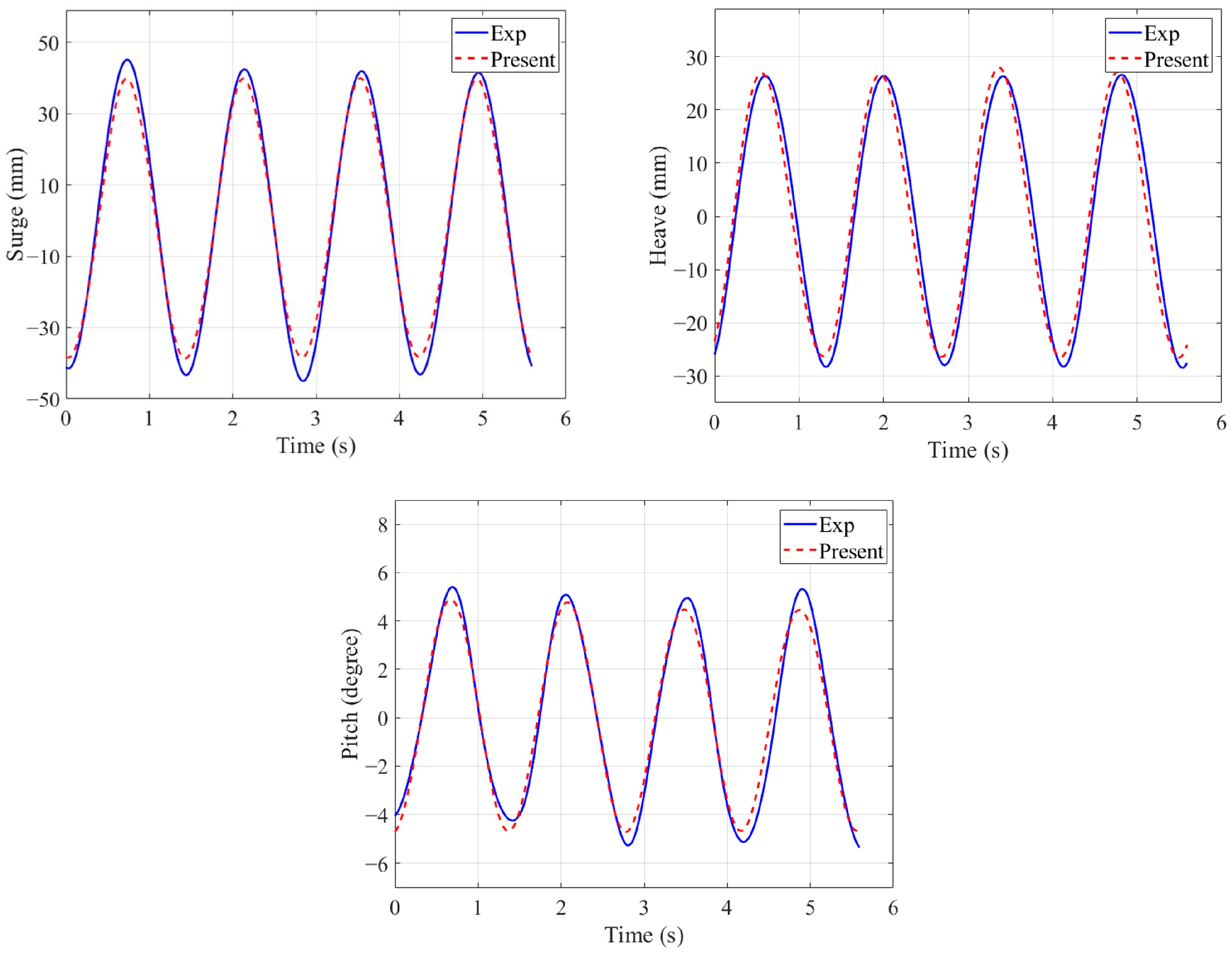
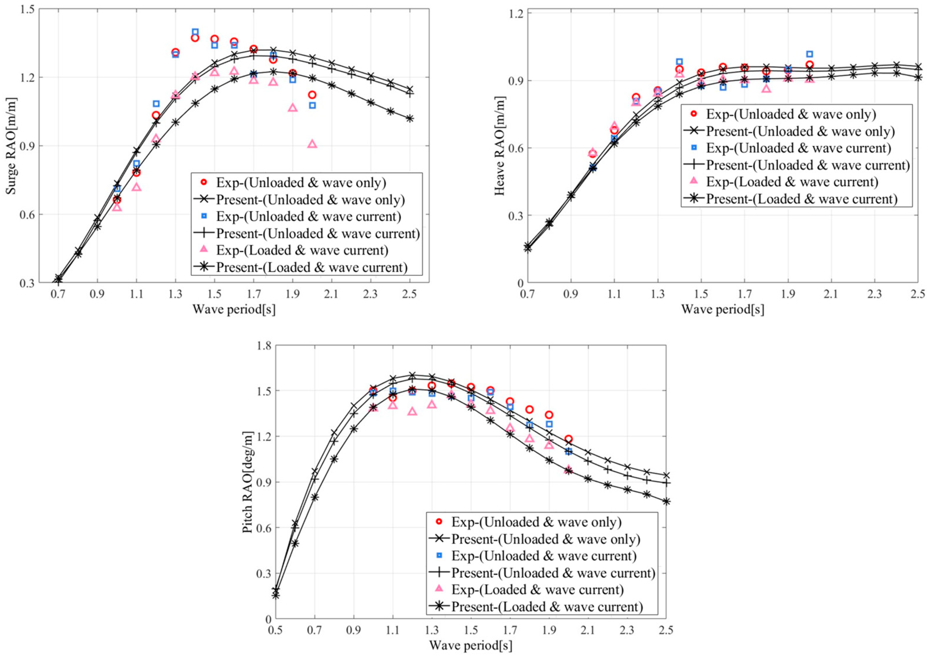
3.4. Verification of Platform Motion Response Results

Figure 5 compares the experimental data of three degrees of freedom (surge, heave, pitch) for a single platform under a wave period of 1.4 s and a wave height of 0.06 m. In the figure, “present” denotes the results of the current model, while “Exp” represents the test results. The accuracy of the numerical simulation is verified, as the simulation shows a periodic repetition of the amplitude and frequency of each movement after the initial transient response, closely aligning with the experimental data. The simulation results closely replicate the experimental findings regarding oscillation amplitudes and periods for surge, heave, and pitch motions. The most significant deviation can be observed in the surge motion, where the model slightly underestimated the response amplitude, though it achieved satisfactory agreement in heave and pitch motions.

Figure 6 illustrates the Response Amplitude Operators (RAOs) for surge, heave, and pitch across wave periods ranging from 0.5 to 2.5 s under consistent wave height conditions. Various scenarios were considered, including wave–current interaction, pure wave conditions, and the presence of a turbine (where unload indicates no turbine installed and load refers to a turbine beneath the floating body). The influence of the turbine on the structural movement was effectively captured, particularly the rotation of the turbine, which reduced the motion amplitude of the platform, as observed in the experiment. Moreover, the motion trends of the three degrees of freedom closely matched the experimental results, especially in rolling and pitching motions. Although the surge motion response simulated by the current model follows the same trend as the test data from the 1.3 s period onward, there is a significant difference in magnitude. The simplified model does not consider the influence of the crossarm between the pontoon bridges, which may result in the tightness of the numerical model during the surge motion.

Figure 7 illustrates the dynamic trajectories under wave–current conditions for two scenarios: platform only and platform with an FTSET device. In both cases, the float trajectories take on an elliptical shape. However, the presence of the turbine amplifies the angles and displacements due to turbine rotation. When the turbine is loaded, the tilt angle of the trajectory relative to the x-axis substantially increases, indicating a shift in the structure’s equilibrium position. As a result, the maximum motion amplitudes for heave and pitch are concentrated in the upper right quadrant. Additionally, the ellipse is oriented from southwest to northeast, reflecting the direction of wave and flow propagation. The elliptical trajectory, especially with the floating turbine, is mainly influenced by the waves.

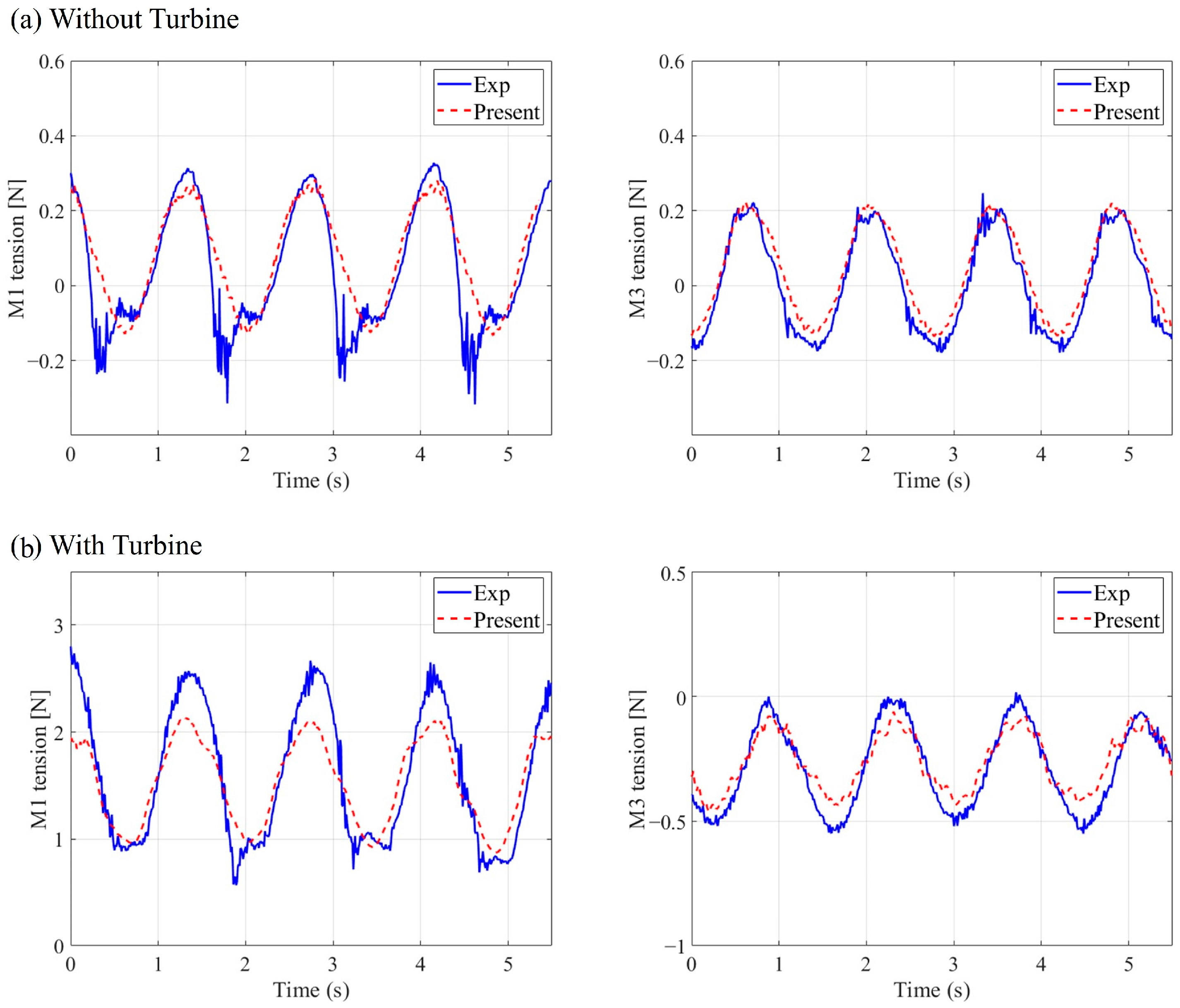
3.5. Verification of Mooring Lines Tension Results

This study critically examines the coupling of mooring dynamics with additional forces induced by the turbine. Figure 8 presents a comparative analysis of tension fluctuations in the mooring lines at the cable attachment point under typical conditions, both with and without the turbine load, through experimental and numerical simulations. To ensure consistency with the experimental setup, the load cell was zeroed in still water. Consequently, the mooring tension value was adjusted by subtracting the pretension in the simulation results, thereby aligning more accurately with the test conditions.

The numerical predictions for mooring forces at the M1 and M3 lines are consistent regarding the period when the turbine is absent. However, the amplitudes are slightly lower, differing by less than 10%, and there was no significant change in instantaneous tension, as noted in studies by Chen et al. [37] and Jeon et al. [44]. With the turbine loaded, the tension in the upstream mooring line (M1 line) significantly increased, exceeding 400% of the tension in the unloaded state, primarily due to the additional forces from turbine rotation. However, the simulations underestimated this increase, capturing only 66% of the experimental value, possibly reflecting the actuator line method’s limitations in accurately simulating turbine forces. Despite these discrepancies, given its computational efficiency and the overall consistency in the magnitude of simulated forces, the approach is considered acceptable for engineering simulations.

Figure 9 displays snapshots of the instantaneous free surface and mooring lines throughout one incident wave period, under constant wave–current parameters (wave height of 0.06 m and wave period of 1.4 s), both with and without the turbine loaded. The color on the free surface, defined at α = 0.5, represents the horizontal velocity values, while the color on the mooring lines indicates the instantaneous tension along each segment.

Initially, the structure underwent a full wave crest-to-trough cycle in scenarios where the turbine was not installed. During the ascent to the wave crest, the mooring forces increased, predominantly supported by the upstream mooring lines. During the descent phase, the tension in the downstream mooring lines exceeded that of the upstream ones, creating a cycle under a balanced state. With the turbine loaded, as shown in Figure 9b, the forces on the upstream mooring lines increased nearly fourfold, causing the equilibrium position of the floating structure to shift backward. Throughout this cycle, the upstream mooring lines consistently endured the majority of the tension, aligning with experimental observations.

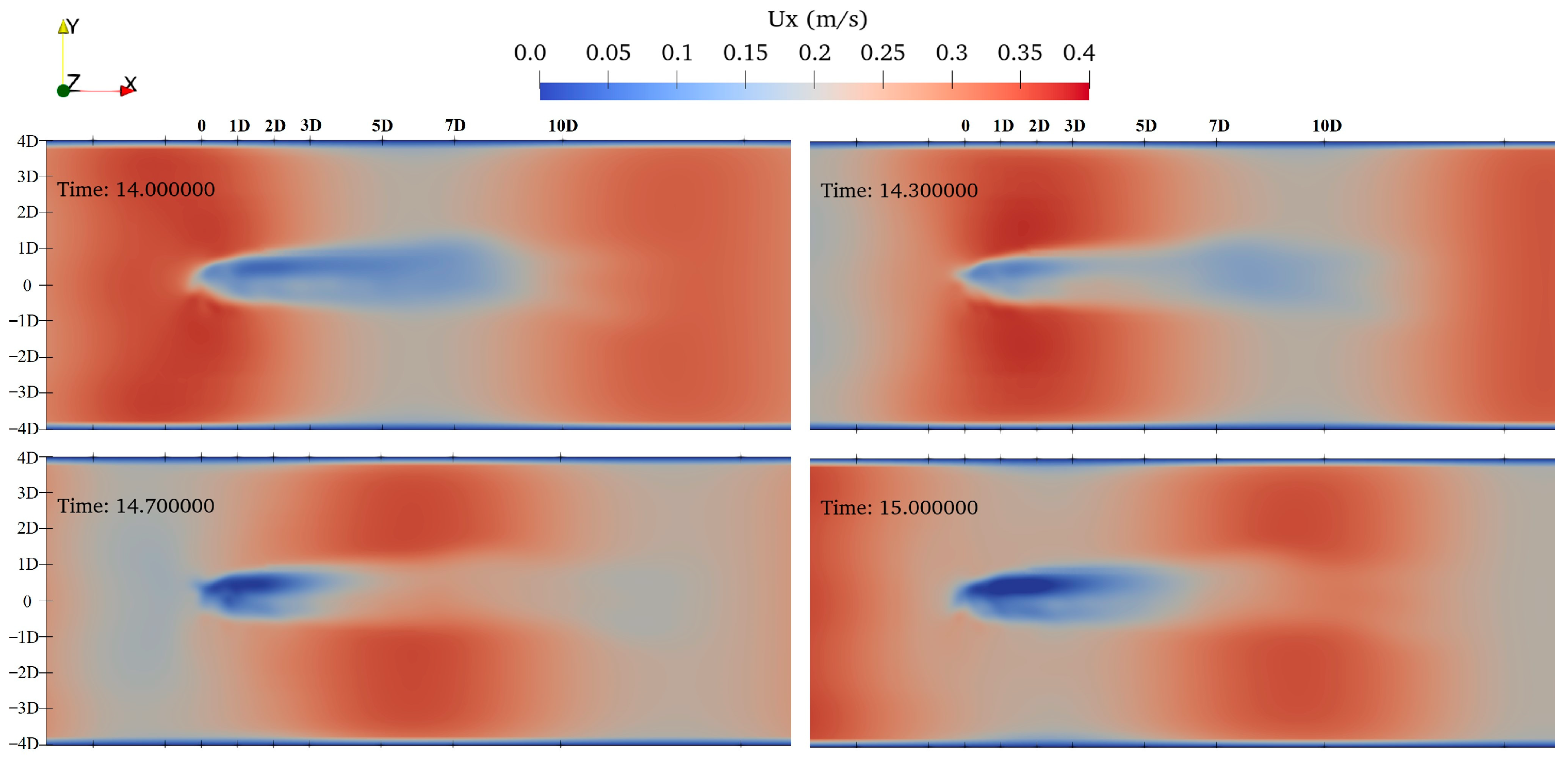
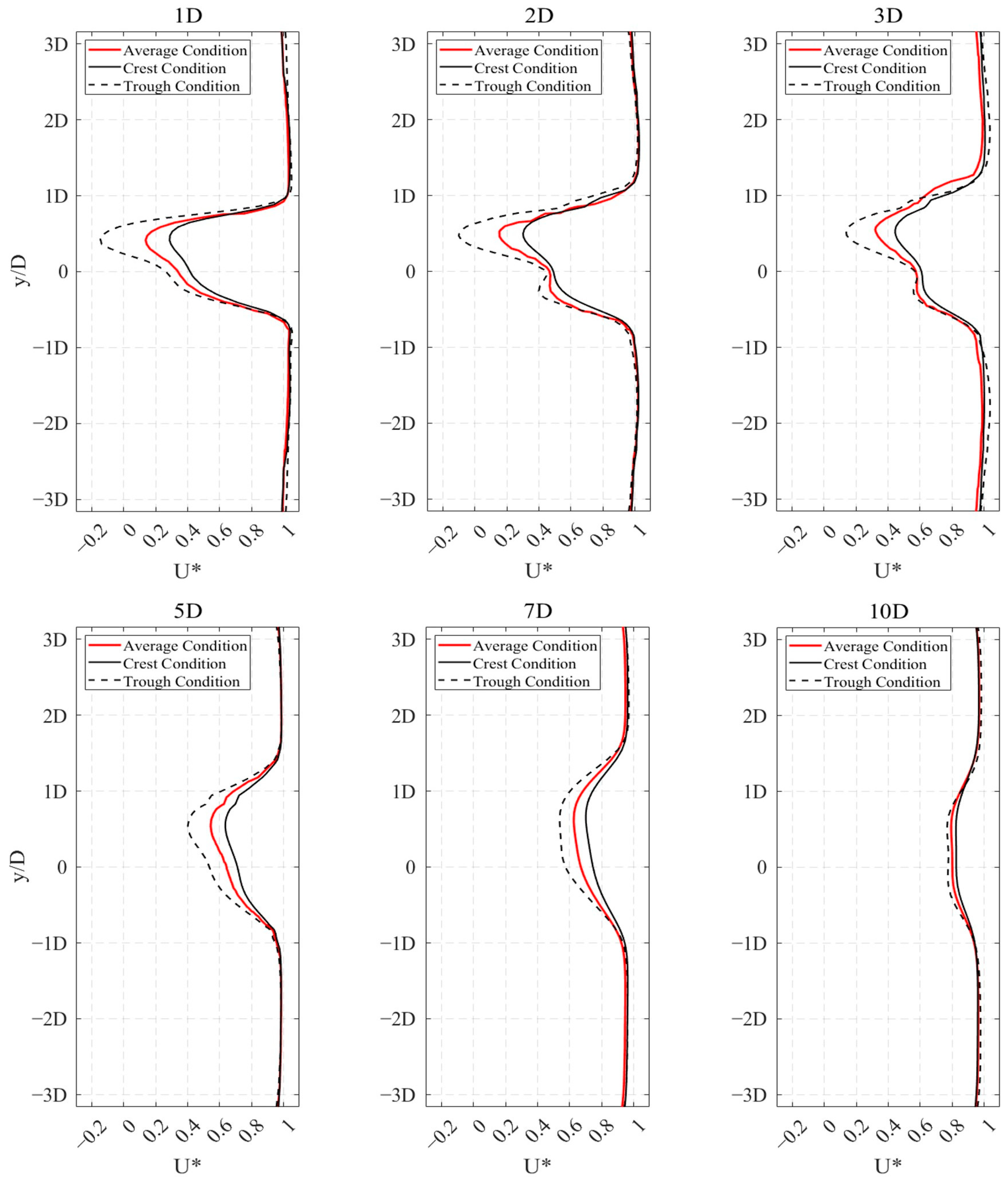
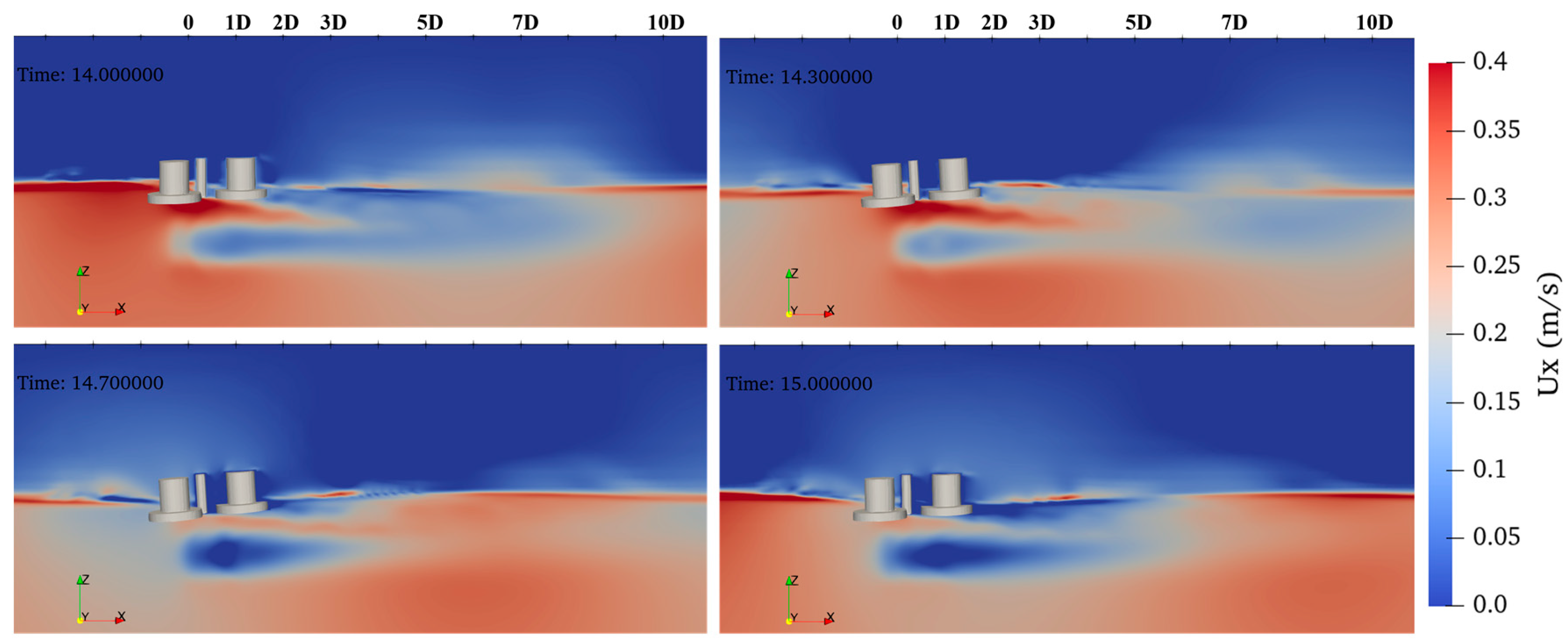
4. Wake Field Characteristics of FTSET

Current coupling models commonly use software such as ANSYS-AQWA [45] and FAST [46] to simulate the motion response of floating structures. However, these models often need to capture the turbulent and disordered flow characteristics typical of natural marine environments. The newly proposed model addresses these limitations. Figure 10 illustrates the development of the turbine wake over a complete incident wave period of 1.4 s, with a wave height of 0.06 m and an average incoming flow velocity of 0.29 m/s, effectively depicting the attenuation induced by the turbine wake. Wave-induced flows led to increased flow velocities at the peak and decreased velocities at the trough, impacting the turbine wake differently than static conditions. The most significant speed reduction occurred approximately 1D to 3D downstream from the turbine, persisting up to 10D. Laterally, the wake diffused significantly, with velocity reductions of up to ±1D. Additionally, velocity superposition effects resulted in a diminished velocity loss when the turbine passed through the crest and an increased loss at the trough. These situations will be further explored in the subsequent quantitative analysis.

Figure 11 illustrates the transverse distribution of the turbine wake. All flow field data have been nondimensionalized for comparative analysis. The peak, trough, and mean flow velocities for corresponding wave conditions have been subtracted to highlight differences between the flow fields. Regardless of the condition, velocity gradually recovered with increasing downstream distance. Velocity reduction was most pronounced in the trough condition, leading to recirculation when x/D was between 1 and 2. Conversely, under peak wave conditions, the magnitude of velocity reduction was less significant, peaking at 31% of the mean flow velocity. By a distance of 10D downstream, the wake had regained approximately 80% of its initial velocity under all three conditions.

Figure 12 illustrates the wake distribution on the xz plane under conditions of a 0.06 m wave height and a 1.4 s wave period. As floating tidal stream turbines were positioned closer to the water surface than fixed turbines to capitalize on higher surface velocities, it is crucial to consider their interaction with the wake of the floating platform structure. Detailed analysis of the wake distribution throughout the incident wave period reveals significant deviations in the flow field. The wake generated by the impeller gradually merged with the platform wake, causing the free liquid surface to shift. The boundary contour of the wake region exhibited a non-smooth, curved pattern, reflecting the periodic motion of the structure.

To quantify the described phenomena of wake development, Figure 13 presents line diagrams at various lateral distances, using dimensionless parameters in the analysis of xy cross-sections. As the wake passed x/D = 1, the Venturi effect increased the flow velocity between the turbine and the structure, shaping the wake profile into an inverted “S” curve. At this point, the maximum flow velocity occurred at the wave peak, reaching 121% of the maximum flow velocity. As the distance downstream increased, the flow field gradually merged, forming a smooth curve by x/D = 7D. At x/D = 10, the wake distribution stabilized at 95%, 89%, and 60% for peak, average, and trough conditions, respectively.

5. Conclusions

This study developed a hybrid numerical model specifically designed to analyze floating tidal stream energy turbine (FTSET) systems. The model integrates a hybrid potential–viscous flow approach with various numerical models, each representing distinct physical domains within the system. For computational fluid dynamics (CFD), grid deformation simulates the floating body’s dynamics in a meticulously constructed three-dimensional numerical wave–current tank powered by olaFlow. The rotor’s dynamics are accurately captured using the refined unsteady actuator line method (UALM), while the complexities of mooring are effectively replicated using the lumped-mass approach of the MoorDyn model. Turbulent phenomena are characterized through the application of the k-ω SST turbulence model.

The model demonstrates remarkable fidelity by accurately replicating the motion responses of the FTSET and aligning closely with the trends in Response Amplitude Operators (RAOs) observed in empirical studies. Although it tends to underestimate mooring line tensions after turbine engagement, the computational predictions exhibit significant correspondence in magnitude with actual measurements. The model’s capability also extends to elucidating wake dynamics, showcasing its comprehensive analytical capacity. Furthermore, the use of a coupling methodology significantly reduces the computational resources required for high-precision simulations. This optimization translates to a more economical modeling approach without sacrificing precision in detailed engineering analyses. Integrating precise motion response simulation with improved wake interaction representation highlights the model’s potential as a transformative tool in engineering. It facilitates the assessment of FTSET systems’ dynamics and offers a cost-efficient alternative for extensive high-fidelity simulations. As such, the model is a pivotal contribution to the evolving field of tidal energy technology, affirming the effectiveness of integrated computational approaches in advancing the design and analysis of renewable energy systems.

References

1. Liu, X.; Chen, Z.; Si, Y.; Qian, P.; Wu, H.; Cui, L.; Zhang, D. A Review of Tidal Current Energy Resource Assessment in China. Renew. Sustain. Energy Rev. 2021, 145, 111012. [Google Scholar] [CrossRef]
2. Liu, Y.; Ma, C.; Jiang, B. Development and the Environmental Impact Analysis of Tidal Current Energy Turbines in China. IOP Conf. Ser. Earth Environ. Sci. 2018, 121, 042003. [Google Scholar] [CrossRef]
3. Zhang, J.; Zhou, Y.; Lin, X.; Wang, G.; Guo, Y.; Chen, H. Experimental Investigation on Wake and Thrust Characteristics of a Twin-Rotor Horizontal Axis Tidal Stream Turbine. Renew. Energy 2022, 195, 701–715. [Google Scholar] [CrossRef]
4. Farkas, A.; Degiuli, N.; Martić, I.; Barbarić, M.; Guzović, Z. The Impact of Biofilm on Marine Current Turbine Performance. Renew. Energy 2022, 190, 584–595. [Google Scholar] [CrossRef]
5. Lamy, J.V.; Azevedo, I.L. Do Tidal Stream Energy Projects Offer More Value than Offshore Wind Farms? A Case Study in the United Kingdom. Energy Policy 2018, 113, 28–40. [Google Scholar] [CrossRef]
6. Zhou, Z.; Benbouzid, M.; Charpentier, J.-F.; Scuiller, F.; Tang, T. Developments in Large Marine Current Turbine Technologies—A Review. Renew. Sustain. Energy Rev. 2017, 71, 852–858. [Google Scholar] [CrossRef]
7. Peng, B.; Zhang, Y.; Zheng, Y.; Wang, R.; Fernandez-Rodriguez, E.; Tang, Q.; Zhang, Z.; Zang, W. The Effects of Surge Motion on the Dynamics and Wake Characteristics of a Floating Tidal Stream Turbine under Free Surface Condition. Energy Convers. Manag. 2022, 266, 115816. [Google Scholar] [CrossRef]
8. Chen, S.; Jiang, B.; Li, X.; Huang, J.; Wu, X.; Xiong, Q.; Parker, R.G.; Zuo, L. Design, Dynamic Modeling and Wave Basin Verification of a Hybrid Wave–Current Energy Converter. Appl. Energy 2022, 321, 119320. [Google Scholar] [CrossRef]
9. Hao, H.; Guo, Z.; Ma, Q.; Xu, G. Air Cushion Barge Platform for Offshore Wind Turbine and Its Stability at a Large Range of Angle. Ocean Eng. 2020, 217, 107886. [Google Scholar] [CrossRef]
10. Shi, J.; Feng, X.; Toumi, R.; Zhang, C.; Hodges, K.I.; Tao, A.; Zhang, W.; Zheng, J. Global Increase in Tropical Cyclone Ocean Surface Waves. Nat. Commun. 2024, 15, 174. [Google Scholar] [CrossRef] [PubMed]
11. Zhang, L.; Wang, S.; Sheng, Q.; Jing, F.; Ma, Y. The Effects of Surge Motion of the Floating Platform on Hydrodynamics Performance of Horizontal-Axis Tidal Current Turbine. Renew. Energy 2015, 74, 796–802. [Google Scholar] [CrossRef]
12. Wang, G.; Zhang, J.; Lu, B.; Lin, X.; Wang, F.; Liu, S. Experimental Investigation of Motion Response and Mooring Load of Semi-Submersible Tidal Stream Energy Turbine under Wave-Current Interactions. Ocean Eng. 2024, 300, 117445. [Google Scholar] [CrossRef]
13. Zhang, Y.; Wei, W.; Zheng, J.; Peng, B.; Qian, Y.; Li, C.; Zheng, Y.; Fernandez-Rodriguez, E.; Yu, A. Quantifying the Surge-Induced Response of a Floating Tidal Stream Turbine under Wave-Current Flows. Energy 2023, 283, 129072. [Google Scholar] [CrossRef]
14. Brown, S.A.; Ransley, E.J.; Greaves, D.M. Developing a Coupled Turbine Thrust Methodology for Floating Tidal Stream Concepts: Verification under Prescribed Motion. Renew. Energy 2020, 147, 529–540. [Google Scholar] [CrossRef]
15. Ma, Y.; Hu, C.; Li, L. Hydrodynamics and Wake Flow Analysis of a Π-Type Vertical Axis Twin-Rotor Tidal Current Turbine in Surge Motion. Ocean Eng. 2021, 224, 108625. [Google Scholar] [CrossRef]
16. Huang, B.; Zhao, B.; Wang, L.; Wang, P.; Zhao, H.; Guo, P.; Yang, S.; Wu, D. The Effects of Heave Motion on the Performance of a Floating Counter-Rotating Type Tidal Turbine under Wave-Current Interaction. Energy Convers. Manag. 2022, 252, 115093. [Google Scholar] [CrossRef]
17. Wang, S.; Li, C.; Zhang, Y.; Jing, F.; Chen, L. Influence of Pitching Motion on the Hydrodynamic Performance of a Horizontal Axis Tidal Turbine Considering the Surface Wave. Renew. Energy 2022, 189, 1020–1032. [Google Scholar] [CrossRef]
18. Chen, S.; Wang, S.; Huang, R.; Shi, W.; Jing, F. Fast Prediction of Hydrodynamic Load of Floating Horizontal Axis Tidal Turbine with Variable Speed Control under Surging Motion with Free Surface. Appl. Ocean. Res. 2023, 135, 103566. [Google Scholar] [CrossRef]
19. Wang, S.; Chen, S.; Li, C.; Guo, W.; Jing, F.; Wang, K. Study on Fast Prediction Method of Hydrodynamic Load of Floating Horizontal Axis Tidal Current Turbine with Pitching Motion under Free Surface. Ocean Eng. 2023, 279, 114589. [Google Scholar] [CrossRef]
20. Zhang, Y.; Peng, B.; Zheng, J.; Zheng, Y.; Tang, Q.; Liu, Z.; Xu, J.; Wang, Y.; Fernandez-Rodriguez, E. The Impact of Yaw Motion on the Wake Interaction of Adjacent Floating Tidal Stream Turbines under Free Surface Condition. Energy 2023, 283, 129071. [Google Scholar] [CrossRef]
21. Brown, S.A.; Ransley, E.J.; Zheng, S.; Xie, N.; Howey, B.; Greaves, D.M. Development of a Fully Nonlinear, Coupled Numerical Model for Assessment of Floating Tidal Stream Concepts. Ocean Eng. 2020, 218, 108253. [Google Scholar] [CrossRef]
22. Brown, S.A.; Ransley, E.J.; Xie, N.; Monk, K.; De Angelis, G.M.; Nicholls-Lee, R.; Guerrini, E.; Greaves, D.M. On the Impact of Motion-Thrust Coupling in Floating Tidal Energy Applications. Appl. Energy 2021, 282, 116246. [Google Scholar] [CrossRef]
23. Bachant, P.; Goude, A.; Wosnik, M. Actuator Line Modeling of Vertical-Axis Turbines. arXiv 2018, arXiv:1605.01449. [Google Scholar]
24. Fleming, P.; Gebraad, P.M.O.; Lee, S.; van Wingerden, J.-W.; Johnson, K.; Churchfield, M.; Michalakes, J.; Spalart, P.; Moriarty, P. Simulation Comparison of Wake Mitigation Control Strategies for a Two-turbine Case. Wind Energ. 2015, 18, 2135–2143. [Google Scholar] [CrossRef]
25. Stanly, R.; Martínez-Tossas, L.A.; Frankel, S.H.; Delorme, Y. Large-Eddy Simulation of a Wind Turbine Using a Filtered Actuator Line Model. J. Wind. Eng. Ind. Aerodyn. 2022, 222, 104868. [Google Scholar] [CrossRef]
26. Deng, X.; Zhang, J.; Lin, X. Proposal of Actuator Line-Immersed Boundary Coupling Model for Tidal Stream Turbine Modeling with Hydrodynamics upon Scouring Morphology. Energy 2024, 292, 130451. [Google Scholar] [CrossRef]
27. Cheng, P.; Huang, Y.; Wan, D. A Numerical Model for Fully Coupled Aero-Hydrodynamic Analysis of Floating Offshore Wind Turbine. Ocean Eng. 2019, 173, 183–196. [Google Scholar] [CrossRef]
28. Yu, Z.; Ma, Q.; Zheng, X.; Liao, K.; Sun, H.; Khayyer, A. A Hybrid Numerical Model for Simulating Aero-Elastic-Hydro-Mooring-Wake Dynamic Responses of Floating Offshore Wind Turbine. Ocean Eng. 2023, 268, 113050. [Google Scholar] [CrossRef]
29. Hall, M.; Goupee, A. Validation of a Lumped-Mass Mooring Line Model with DeepCwind Semisubmersible Model Test Data. Ocean Eng. 2015, 104, 590–603. [Google Scholar] [CrossRef]
30. Higuera, P.; Losada, I.J.; Lara, J.L. Three-Dimensional Numerical Wave Generation with Moving Boundaries. Coast. Eng. 2015, 101, 35–47. [Google Scholar] [CrossRef]
31. Hirt, C.W.; Nichols, B.D. Volume of Fluid (VOF) Method for the Dynamics of Free Boundaries. J. Comput. Phys. 1981, 39, 201–225. [Google Scholar] [CrossRef]
32. Gatin, I.; Vukčević, V.; Jasak, H.; Rusche, H. Enhanced Coupling of Solid Body Motion and Fluid Flow in Finite Volume Framework. Ocean Eng. 2017, 143, 295–304. [Google Scholar] [CrossRef]
33. Mentes, A.; Yetkin, M. An Application of Soft Computing Techniques to Predict Dynamic Behaviour of Mooring Systems. Brodogradnja 2022, 73, 121–137. [Google Scholar] [CrossRef]
34. Wang, B.; Jiao, Y.; Qiao, D.; Gao, S.; Li, T.; Ou, J. Motion Characteristics of Vertically Loaded Anchor during Drag Embedment in Layered Clay. Brodogradnja 2023, 74, 109–125. [Google Scholar] [CrossRef]
35. Palm, J.; Eskilsson, C.; Paredes, G.M.; Bergdahl, L. Coupled Mooring Analysis for Floating Wave Energy Converters Using CFD: Formulation and Validation. Int. J. Mar. Energy 2016, 16, 83–99. [Google Scholar] [CrossRef]
36. Lee, S.C.; Song, S.; Park, S. Platform Motions and Mooring System Coupled Solver for a Moored Floating Platform in a Wave. Processes 2021, 9, 1393. [Google Scholar] [CrossRef]
37. Chen, H.; Hall, M. CFD Simulation of Floating Body Motion with Mooring Dynamics: Coupling MoorDyn with OpenFOAM. Appl. Ocean. Res. 2022, 124, 103210. [Google Scholar] [CrossRef]
38. Johlas, H.M.; Martínez-Tossas, L.A.; Lackner, M.A.; Schmidt, D.P.; Churchfield, M.J. Large Eddy Simulations of Offshore Wind Turbine Wakes for Two Floating Platform Types. J. Phys. Conf. Ser. 2020, 1452, 012034. [Google Scholar] [CrossRef]
39. Devolder, B.; Rauwoens, P.; Troch, P. Application of a Buoyancy-Modified k-ω SST Turbulence Model to Simulate Wave Run-up around a Monopile Subjected to Regular Waves Using OpenFOAM®. Coast. Eng. 2017, 125, 81–94. [Google Scholar] [CrossRef]
40. Devolder, B.; Troch, P.; Rauwoens, P. Performance of a Buoyancy-Modified k-ω and k-ω SST Turbulence Model for Simulating Wave Breaking under Regular Waves Using OpenFOAM®. Coast. Eng. 2018, 138, 49–65. [Google Scholar] [CrossRef]
41. Dai, P.; Huang, Z.; Zhang, J. A Modelling Study of the Tidal Stream Resource around Zhoushan Archipelago, China. Renew. Energy 2023, 218, 119234. [Google Scholar] [CrossRef]
42. Pericàs, P.F. CFD Simulation of a Floating Wind Turbine with OpenFOAM: An FSI Approach Based on the Actuator Line and Relaxation Zone Methods. Master’s Thesis, Delft University of Technology, Delft, The Netherlands, 2022. [Google Scholar]
43. Domínguez, J.M.; Crespo, A.J.C.; Hall, M.; Altomare, C.; Wu, M.; Stratigaki, V.; Troch, P.; Cappietti, L.; Gómez-Gesteira, M. SPH Simulation of Floating Structures with Moorings. Coast. Eng. 2019, 153, 103560. [Google Scholar] [CrossRef]
44. Jeon, W.; Park, S.; Cho, S. Moored Motion Prediction of a Semi-Submersible Offshore Platform in Waves Using an OpenFOAM and MoorDyn Coupled Solver. Int. J. Nav. Archit. Ocean. Eng. 2023, 15, 100544. [Google Scholar] [CrossRef]
45. Wan, D.; Zhao, W. Numerical Study of Interactions Between Phase II of OC4 Wind Turbine and Its Semi-Submersible Floating Support System. J. Ocean. Wind. Energy 2015, 2, 45–53. [Google Scholar]
46. Dunbar, A.J. Development and Validation of a Tightly Coupled CFD/6-DOF Solver for Simulating Floating Offshore Wind Turbine Platforms. Ocean Eng. 2015, 110, 98–105. [Google Scholar] [CrossRef]
Figure 1. Schematic diagram of the computational domain.
Jmse 12 01046 g001
Figure 2. Flow chart of the FTSET fully coupled model.
Jmse 12 01046 g002
Figure 3. Diagram of mooring line facilities.
Jmse 12 01046 g003
Figure 4. Schematic diagram of the computational domain, (a) computational domain, (b) wake area meshing, (c) floating body meshing.
Jmse 12 01046 g004
Figure 5. Comparison of the platform motion response in regular wave case (WT = 1.4 s, Wh = 0.06 m).
Jmse 12 01046 g005
Figure 6. Comparison of the platform Response Amplitude Operators (RAOs) curves in a regular wave.
Jmse 12 01046 g006
Figure 7. Motion attitude and trajectory of the platform in wave–current case (WT = 1.4 s, Wh = 0.06 m).
Jmse 12 01046 g007
Figure 8. Comparison of mooring anchor tensions in the M1 and M3 lines in wave–current case (WT = 1.4 s, Wh = 0.06 m).
Jmse 12 01046 g008
Figure 9. Schematic diagram of instantaneous surface velocity and mooring tension in a wave period: (a) without turbine; (b) with turbine.
Jmse 12 01046 g009
Figure 10. The contours of velocity deficit on XY profile (WT = 1.4 s, Wh = 0.06 m).
Jmse 12 01046 g010
Figure 11. Lateral velocity distribution under crest, trough, and average conditions (WT = 1.4 s, Wh = 0.06 m).
Jmse 12 01046 g011
Figure 12. The contours of velocity deficit on the xz profile (WT = 1.4 s, Wh = 0.06 m).
Jmse 12 01046 g012
Figure 13. Vertical velocity distribution under crest, trough, and average conditions (WT = 1.4 s, Wh = 0.06 m).
Jmse 12 01046 g013