Analysis of the Bending Height of Flexible Marine Vegetation

Abstract

Marine vegetation is increasingly viewed as a living shoreline that protects coastal communities and ecosystems from the damaging effects of wave energy. Many studies have explored the potential of marine vegetation in terms of reducing wave height, but more work is needed. Here, we used particle image velocimetry, fluid–structure interaction simulation, and multiple regression analysis to estimate the bending behaviors of flexible marine vegetation in water flow, and we predicted the wave height reduction in the downstream vegetation meadow. We considered different vegetation types and water flow velocities, constructed a total of 64 cases, and derived a multiple regression equation that simply estimates the vegetation bending height with a tolerance of ~10%. When the bending height rather than the vegetation height was applied, wave height reduction was alleviated by 1.08–9.23%. Thus, flexible vegetation reduced wave height by up to ~10% less than rigid vegetation in our investigation range. This implies that the impact of bending behavior becomes more pronounced with a larger vegetation meadow. The relative % decrease in wave height reduction was greater for fully submerged vegetation compared to partially submerged vegetation.

1. Introduction

Considerable efforts have been made over the past few decades to investigate the effects of climate change on coastal and terrestrial vegetation. These studies were conducted to better understand how environmental changes (e.g., temperature) affect vegetation covers and distributions [1,2,3,4]. Significant efforts have also been made to explore the impacts of marine vegetation (e.g., seagrass, mangroves, salt marshes, kelp, and red algae) on the aquatic environment. Such studies have sought to better understand how marine vegetation regulates fluid flow patterns [5,6,7,8] and the transport of nutrients, pollutants, and sediments [9,10,11,12]. Using various tools and techniques, researchers have explored the complex interactions between marine vegetation and fluid flow, yielding insights into the ecological and environmental benefits afforded by such ecosystems. Research in this area is becoming increasingly important in terms of protecting and preserving the health of the oceans and coastal areas.

Waves tend to increase in height as they approach the shore, triggering erosion and other damage to coastal habitats and infrastructure. Marine vegetation meadows serve as natural barriers that slow waves and reduce wave energies and heights [13,14]. This not only protects against erosion but also provides habitats for many marine species. The roots of marine vegetation stabilize the sediments; these are then not washed away by strong currents or storms [15,16]. Today, marine vegetation is increasingly viewed as a living shoreline that protects coastal communities and ecosystems from the damaging effects of wave energy [14,17]. To explore how marine vegetation reduces wave height or energy, laboratory-scale experiments [18,19,20], field experiments [21,22], simulations [23,24], and theoretical calculations [25] have been employed using either living [26] or artificial [20,27] vegetation. Some studies used simple computations that treated vegetation as completely rigid [25,28,29], thus ignoring real-world flexibility. Other studies indeed investigated flexible vegetation [13,27], but only a few specific types. The distinction between rigid and flexible vegetation lies in their motion. Flexible vegetation can bend and sway in response to water flow forces, while rigid vegetation tends to maintain its original posture. Various studies have explored the movement of vegetation, revealing its significant impact on wave attenuation within vegetation meadows by reducing drag [30,31,32,33]. A more general method is needed to quantify how flexible vegetation reduces wave height. There is a need for a more widely accepted approach, such as simulation, which has broad applicability, or an empirical equation to address this complexity.

Here, we studied the bending behaviors and reduced heights of flexible marine vegetation under water flow and predicted wave height reductions in the downstream vegetation meadow. This approach may optimally address how vegetation reduces wave height because it considers a reduced vegetation height (i.e., the bending height) rather than the original height (i.e., the vegetation height). We first used particle image velocimetry (PIV) in the laboratory to determine the bending height. We confirmed the results via fluid–structure interaction (FSI) simulation using the ANSYS Fluent software 2023 R1 package (ANSYS, Inc., Canonsburg, PA, USA). Based on the data obtained, we established a multiple regression equation that rather simply yields the bending heights. We used these values to derive the wave height reductions downstream and compared the results to those obtained using the vegetation heights. The contribution of this study can be highlighted as follows. First, we estimated the bending behaviors of flexible vegetation in water flow; the estimated equation was effective in calibrating the vegetation height due to bending behavior. Second, we predicted the effect of bending behavior on wave height; rigid vegetation proved to be more effective in reducing wave height than flexible vegetation. Finally, we observed that the relative % decrease in wave height reduction is greater for fully submerged vegetation compared to partially submerged vegetation.

2. Materials and Methods

2.1. Artificial Vegetation

Table 1. Artificial vegetation and their properties that have been investigated in previous studies. Note that the notation “–” indicates that the relevant information was not given, and the footnote shows the vegetation type used in the authors’ experiment.

Vegetation † Shape			Density	Young’s Modulus (MPa)	Material Type	References
Height (m)	Width or Diameter (mm)	Thickness (mm)
0.15–0.50	10	~0.2	900 ± 20	540 ± 10	Polyethylene	[35]
0.30	12	–	32	–	Polyethylene	[18]
0.30	12	–	–	–	Wooden dowel
0.55	–	1.0	550–700	903	Polypropylene	[20]
0.10–0.15	1.8–2.2	–	–	–	Cable ties	[36]
0.10–0.30	1.8–2.2	–	–	–	Poly ribbon
0.55	10	1.0	550–700	903	PVC	[19]
0.21	4.0	0.1	800	600	Polyethylene	[13]
0.16	10	0.25	–	300	LDPE	[37]
0.07	6.35	–	–	–	Wooden dowel
0.07	38.1	–	–	–	PVC
0.45	–	–	–	645 ± 10	HDPE	[29]
0.45	–	–	–	3530 ± 390	PVC
0.45	–	–	–	196 ± 49	Polyethylene
0.30	5.0	–	350	2917	Bamboo dowel	[34]
0.30	5.0	–	998	0.56	Silicon sealant

^† The target vegetation species: P. oceanica [19,20,35], S. alterniflora [18], Z. noltii [36], E. acoroides [13], T. testudinum [37], and Rhizophora [29].

lists the vegetation species examined in published studies; these varied widely in terms of vegetation height (0.07–0.55 m), width (1.8–38.1 mm), and Young’s modulus (0.56–3530 ± 390 MPa). The table also lists the comparable features of alternative (or artificial) materials used. For example, materials used to represent artificial rigid or flexible vegetables included polyethylene [18], polyvinyl chloride [19], and bamboo dowels with silicon sealants [34]. It is difficult to perform experiments using live vegetation; real plants are irregular in shape, susceptible to weather conditions, and decompose within a few days after removal from the natural environment. We used thin polystyrene, a synthetic polymer of styrene (an aromatic hydrocarbon) monomers, to simulate the behaviors of real vegetation in water flow; the characteristics are listed in

Table 2. The characteristics of polystyrene used in this study.

Property	Magnitude	Unit
Density	1040	kg m−3
Coefficient of Thermal Expansion	0.00016	°C−1
Young’s Modulus	2.73 × 109	Pa
Poisson’s Ratio	0.395	-
Bulk Modulus	4.3333 × 109	Pa
Shear Modulus Tensile Yield Strength	9.7849 × 108 3.45 × 107	Pa Pa
Tensile Ultimate Strength	4.31 × 107	Pa

. We created nine types of artificial vegetation by fixing the thickness (0.001 m) and changing the height (0.250, 0.300, and 0.350 m) and width (0.010, 0.015, and 0.020 m).

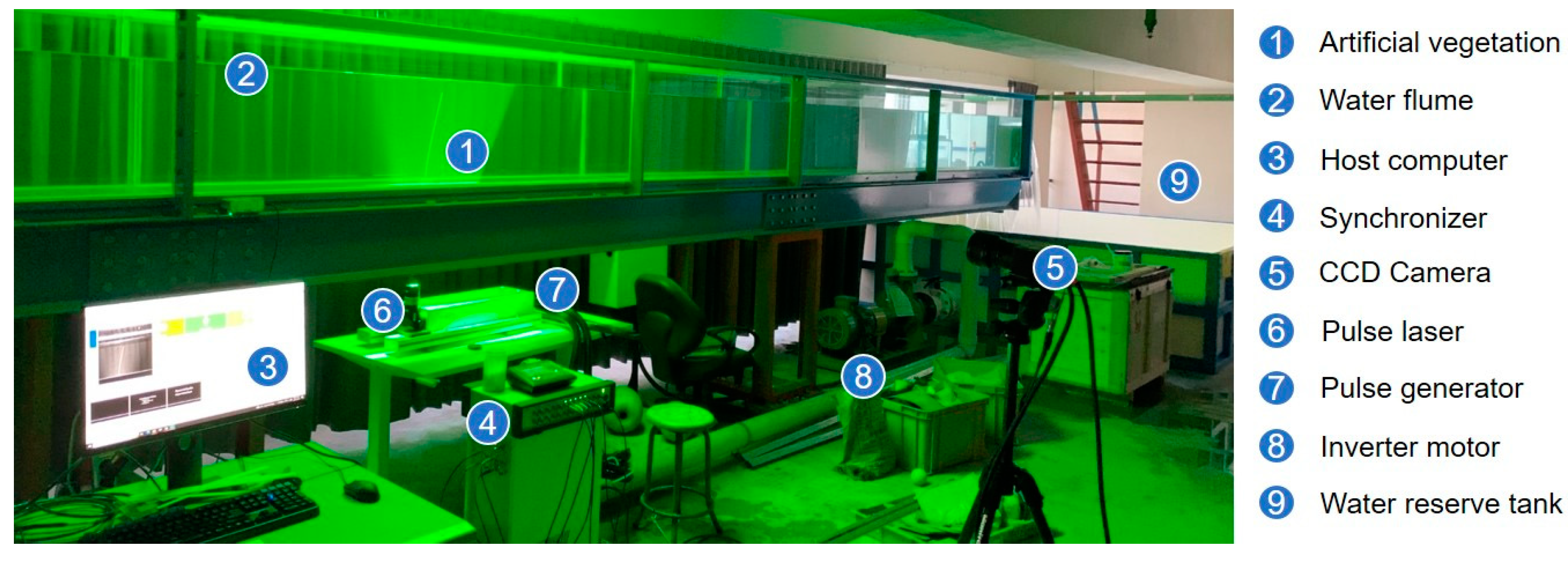
2.2. Experimental Setup

We performed PIV to quantify the bending heights. PIV is a form of optical measurement that instantaneously measures the velocity field in a flow region [38,39]. In a typical PIV experiment, a fluid is illuminated using a pulsed laser light that is scattered by small tracer particles in the fluid, and then the flow field is captured in two images of a high-speed camera taken at two different times during the laser pulse [40]. Figure 1 shows the experimental setup comprising a PIV pulse laser unit (DualPower 200-15; Dantec, Skovlunde, Denmark), pulse generator, synchronizer, charge-coupled device (CCD) camera with a 15 Hz sampling rate (EO 4M-32 FlowSense; Dantec; Skovlunde, Denmark), and host computer.

The seed particles were hollow and smooth borosilicate glass spheres that both followed the flow and scattered light that was captured by the CCD camera, which converted the light intensities into electrical signals stored in computer memory after analog-to-digital conversion. The synchronizer timed the PIV system’s operation; imaging and laser lighting operated simultaneously. The computer featured PIV software (DynamicStudio 7.0) that processed the image pairs to produce velocity flow maps. The micron-sized seed particles scattered light that was imaged using a laser light sheet less than 1 mm in thickness.

The water flume (0.5 m wide, 0.5 m high, and 10.0 m long) was made of steel and tempered glass. When choosing the water flow velocity, we considered previous studies that employed 0.08–0.25 m s⁻¹ [35] and 0.1–0.2 m s⁻¹ [41] to replicate real-world flows by location and season. We used velocities of 0.089–0.155 m s⁻¹, thus within the abovementioned ranges for coastal environments. We used an inverter motor attached to a water tank (Figure 1). At rotation frequencies of 30, 40, and 50 Hz, the flow velocities were 0.089, 0.123, and 0.155 m s⁻¹, respectively.

Using these three water velocities and nine types of artificial vegetation, we evaluated 27 experimental cases (

Table 3. The characteristics of polystyrene used in this study. The density, Young’s modulus, and thickness of the polystyrene are fixed as 1040 kg m⁻³, 2.73 × 10⁹ Pa, and 0.001 mm, respectively.

No.	Height (m)	Width (m)	Inlet Velocity (m s−1)	No	Height (m)	Width (m)	Inlet Velocity (m s−1)
Exp_01	0.250	0.020	0.089	Exp_15	0.300	0.010	0.123
Exp_02	0.250	0.015	0.089	Exp_16	0.350	0.020	0.123
Exp_03	0.250	0.010	0.089	Exp_17	0.350	0.015	0.123
Exp_04	0.300	0.020	0.089	Exp_18	0.350	0.010	0.123
Exp_05	0.300	0.015	0.089	Exp_19	0.250	0.020	0.155
Exp_06	0.300	0.010	0.089	Exp_20	0.250	0.015	0.155
Exp_07	0.350	0.020	0.089	Exp_21	0.250	0.010	0.155
Exp_08	0.350	0.015	0.089	Exp_22	0.300	0.020	0.155
Exp_09	0.350	0.010	0.089	Exp_23	0.300	0.015	0.155
Exp_10	0.250	0.020	0.123	Exp_24	0.300	0.010	0.155
Exp_11	0.250	0.015	0.123	Exp_25	0.350	0.020	0.155
Exp_12	0.250	0.010	0.123	Exp_26	0.350	0.015	0.155
Exp_13	0.300	0.020	0.123	Exp_27	0.350	0.010	0.155
Exp_14	0.300	0.015	0.123

). Each vegetation was installed in the center of the flume, and five measurements were obtained at each water flow velocity to confirm reproducibility. No waves were generated, and all vegetation was fully submerged in the flume. The dimensions of the velocity profile mapping region were 27 L × 33 L, where L = 10.765 mm, and that region was vertically divided into ten local locations, thus from line 0 L to line 27 L at intervals of 3 L. Accordingly, ten local velocities, from $u_1$ to $u_{10}$, were obtained (Figure 2a); the window used to measure water velocity was ~290 × 355 mm (Figure 2b). The laser illuminated the vegetation, and the CCD camera captured vegetation movement and velocity. We obtained the bending heights (i.e., the heights after bending by the water flow) by observing the deformations apparent on PIV images when the deformation had stabilized.

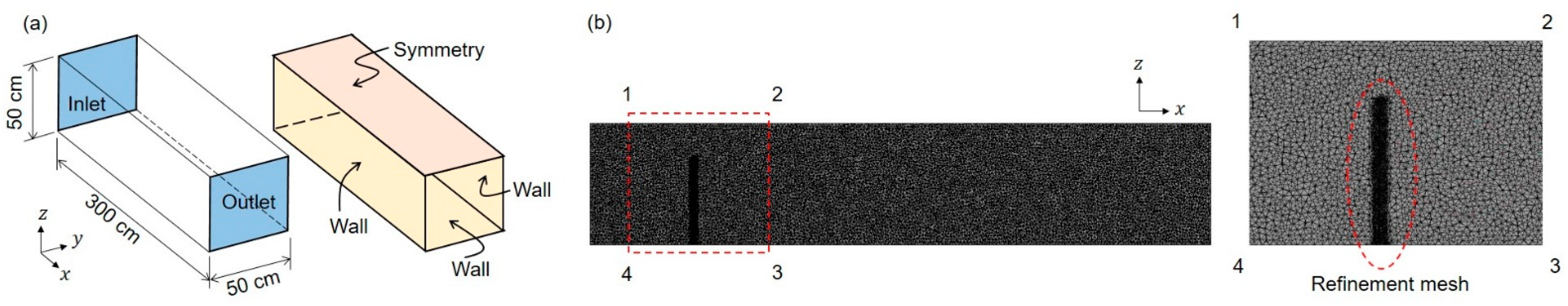
2.3. Fluid–Structure Interaction Simulation

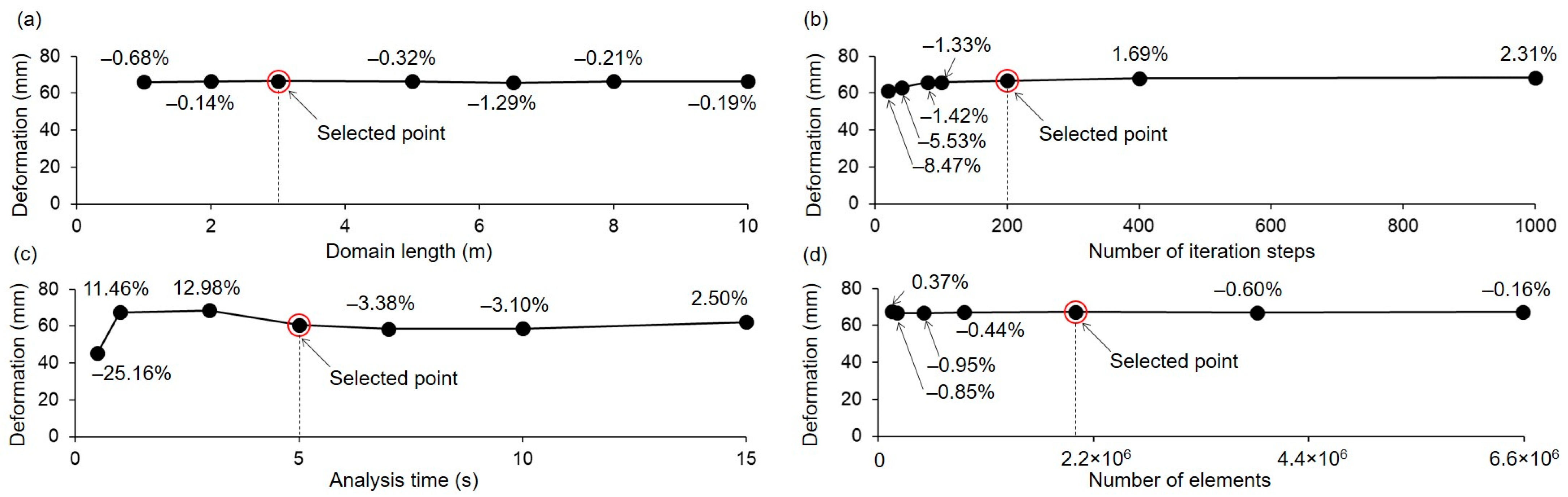
FSI refers to the interaction between a movable or deformable structure and an internal or surrounding fluid flow. In general, an FSI problem is structured to ensure that the field equations for the solid and fluid affect and modify each other. A solid not only induces fluid motion but also modifies that motion by creating stresses at the solid–fluid interface [42]. Two conditions must be met when balancing the motions of a solid and a fluid. First, the solid and fluid movements must match at the interface. Second, the mutual forces exerted at the interface must be equal. In an FSI simulation, the fluid and solid fields are solved independently at each time step and then coupled until the required conditions at the interface are satisfied. Initially, the pressure from the fluid field affects the solid, causing the solid to deform or move; these changes are then back-transferred to the fluid field, changing the properties thereof [43]. A calculation cycle is complete when the modified pressure again affects the solid. FSI simulations effectively model the real behaviors of flexible objects and their surrounding environments and have thus found applications in automobile, aircraft, spacecraft, engine, bridge design, and medical fields [44,45,46].

The FSI equation is then combined with the equations governing the fluid and structure domains [47]. The fluid domain is described using Navier–Stokes, continuity, volume fraction, and energy equations, as shown in Equations (1)–(4), respectively:

$$\frac{\partial }{\partial t}\left(\rho \overrightarrow{v}\right)+\nabla ·\left(\rho \overrightarrow{v}\overrightarrow{v}\right)=-\nabla p+\nabla ·\left(\overline{\overline{\tau }}\right)+\rho \overrightarrow{g}+\overrightarrow{F}$$

(1)

$$\frac{\partial \rho }{\partial t}+\nabla ·\left(\rho \overrightarrow{v}\right)=S_m$$

(2)

$${{\displaystyle \sum }}_{q=1}^n{\alpha }_q=1$$

(3)

$$\frac{\partial }{\partial t}\left(\rho E\right)+\nabla ·\left(\overrightarrow{v}\left(\rho E+p\right)\right)=\nabla ·\left(k_{\mathrm{eff}}\nabla T-{\displaystyle \sum }_j{h}_j\overrightarrow{J}+{\overline{\overline{\tau }}}_{\mathrm{eff}}.\overrightarrow{v}\right)+S_h$$

(4)

where $t$ is time, $\rho$ the fluid density, $\overrightarrow{v}$ the velocity vector, $\nabla$ the gradient, $p$ the pressure, $\overline{\overline{\tau }}$ the stress tensor, $\overrightarrow{g}$ gravitational acceleration, $\overrightarrow{F}$ an external body force vector, $S_m$ a mass source term, $\alpha$ the fluid volume fraction, $E$ the total energy, $k_{\mathrm{eff}}$ the effective fluid thermal conductivity, $T$ the temperature, $h$ the enthalpy, $\overrightarrow{J}$ the diffusion flux vector, ${\overline{\overline{\tau }}}_{\mathrm{eff}}$ the viscous stress tensor, and $S_h$ a volumetric energy source. The computational model of the solid domain features three-dimensional strain and nodal displacement equations, and a stress equation [47], as shown in Equations (5)–(7):

$$\left[B\right]=[\partial ]\left[N\right]$$

(5)

$$\left\{\epsilon \right\}=\left[B\right]\left\{D\right\}$$

(6)

$$\left\{\sigma \right\}=\left[E\right]\left\{\epsilon \right\}$$

(7)

where $B$ is the strain displacement, $\partial$ the four-dimensional gradient (time and space), $N$ an element shape function, $\epsilon$ the strain, $D$ the nodal displacement, $\sigma$ the stress, and $E$ the modulus of elasticity.

2.4. Simulation

We performed an FSI simulation to evaluate the experimental results. To model turbulence, the Reynolds stress model was chosen because it is both reliable and cost-effective [48]. We used the “transient structural module” and the “fluent module”. The former module determines the displacement or deformation of a solid body caused by fluid pressure within the domain. The result is then transferred to the fluent module, which re-calculates the characteristics of the fluid domain. Finally, all results are back-transferred to the solid body; this completes the cycle. The following assumptions were made. First, for the transient structural module, the vegetation was assumed to be uniform in terms of shape and homogeneous; the shape did not change from bottom to top, and the properties thereof were identical throughout the vegetation height. We also assumed that the connection between vegetation and the seabed was rigid; we thus imposed a fixed-support boundary condition. Five surfaces of each vegetation, including the front, back, two sides, and the top, served as the interfaces between the fluid domain and the vegetation. Finally, it was assumed that the seabed was absolutely flat, and friction occurred between the flow and the seabed.

We carefully considered the modeling parameters; we performed tests that independently identified a reasonable domain length, the number of iteration steps, the analysis time, and the number of elements (Figure 3). In this figure, the percentage represents the relative error between the current deformation of the calculation point ($D_{cal}$) and the selected point ($D_{sel}$) and is defined by $\left(D_{cal}-D_{sel}\right)/D_{sel}\times 100(\%)$. The top, horizontal vegetation deformation reached convergence values at an early stage with respect to the domain length and number of elements, respectively. However, the deformation was sensitive to the number of iteration steps and analysis time; hence, the selected points were determined to minimize the relative errors of the calculation points. As a result, we chose a domain length of 3.0 m, 200 iteration steps, an analysis time of 5 s, and ~2 million elements. The domain height and width were the actual dimensions of the rectangular flume (50 cm in height and 50 cm in width).

The boundary conditions included an inlet, an outlet, symmetry, and a no-slip wall (Figure 4a). The inlet was the boundary from which the flow entered; the inlet flow velocity was 0.089, 0.123, or 0.155 m s⁻¹, identical to those of the PIV experiments. The outlet boundary forced the flow to exit through an outlet. The symmetry condition ensured that the physical geometry and the anticipated flow pattern exhibited mirror symmetry [49]. The no-slip wall condition was applied to the lateral and bottom sides. We created mesh layers, gradually decreasing the mesh size from 15 mm in the fluid domain to 5 mm in the solid domain (each vegetation) (Figure 4b). A tetrahedral mesh was used because this is optimal in terms of automated meshing, stress visualization, and predictions of contact pressure and shear stress [50].

We used three dynamic mesh schemes: smoothing, layering, and re-meshing to explore the movements of individual vegetation [39]. Smoothing enables adjustment of a zone mesh by deforming or moving the boundary; the interior mesh nodes are displaced, but the node number is maintained, as are all connections. Dynamic layering facilitates the specification of an ideal layer height for each moving boundary. Re-meshing involves the clustering of cells that fail to meet skewness or size criteria; such cells or faces are subsequently re-meshed [51]. We used WebplotDigitizer to extract vegetation bending heights [52].

3. Results

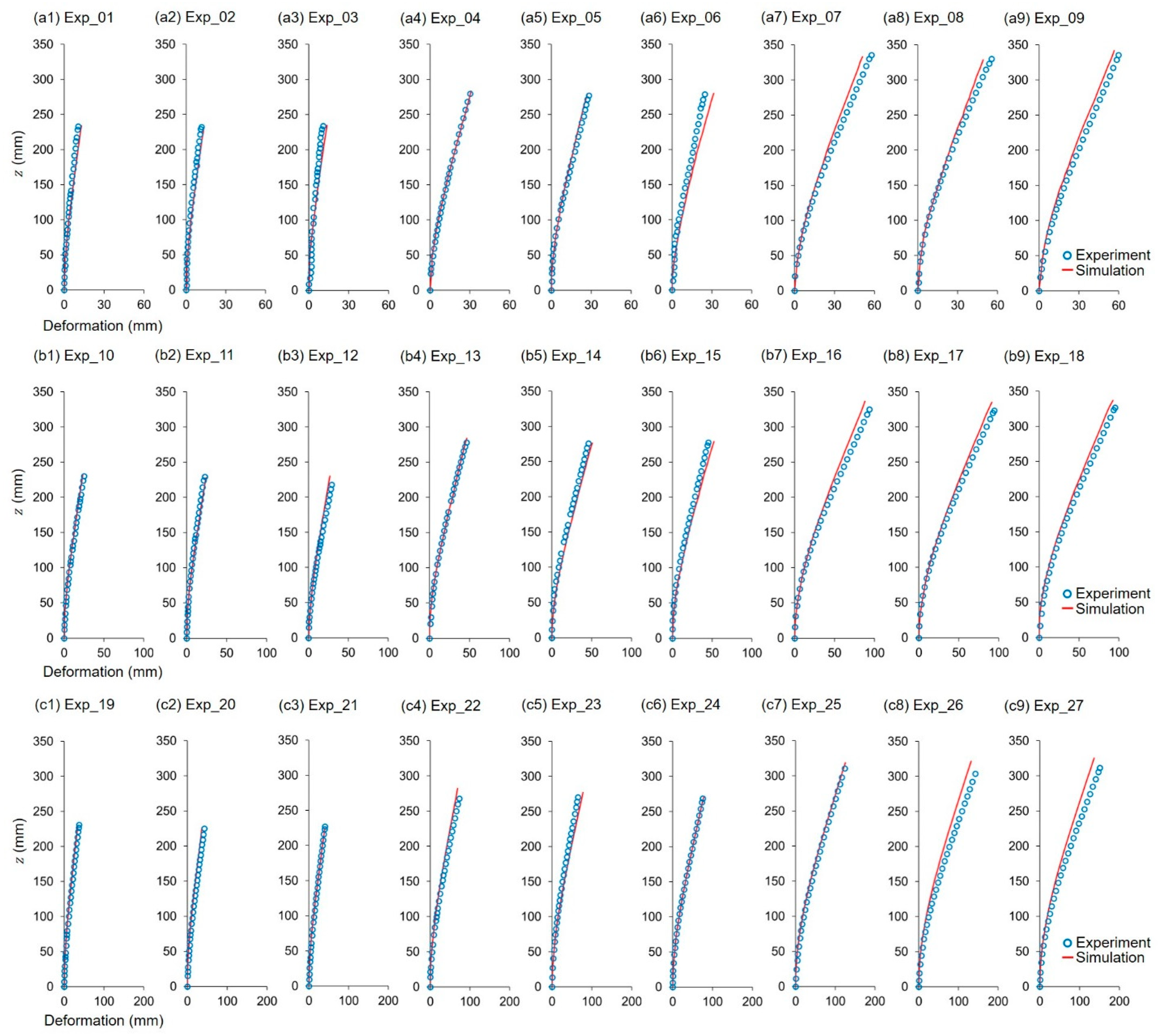
3.1. Experimental and Simulation Results

Figure 5(a1–a10) show ten local velocity distributions at an inlet velocity of 0.089 m s⁻¹ measured at ten vertical lines (Figure 2a). The horizontal axis indicates the normalized velocity $u_i/V_j$, which is the ratio of each local velocity at the $i^{th}$ vertical line to the inlet velocity $V_j$. Here, $i$ ranges from 1 to 10 and $j$ from 1 to 3 (e.g., $V_1$ = 0.089 m s⁻¹). The vertical axis indicates the vertical location from 0 to 33 L (Figure 2a). Similarly, Figure 5(b1–b10,c1–c10) show the velocity profiles for $V_2$ = 0.123 m s⁻¹ and $V_3$ = 0.155 m s⁻¹, respectively. In each figure, the velocity near the boundary (the bottom of the flume) is smaller than elsewhere because of friction between the water flow and the bottom of the flume.

Table 4. Bending height ($h_b$) of vegetation obtained from the PIV measurement and FSI simulation. The relative % differences are with respect to the vegetation heights ($h_v$), i.e., $\left(h_b-h_v\right)/h_v\times 100\%$; the relative % errors are with respect to the bending heights obtained from the PIV measurement (to be continued).

Case	${\mathit{h}}_{\mathit{v}}$ (m)	PIV Measurement		FSI Simulation
		${\mathit{h}}_{\mathit{b}}$ (m)	Rel. % Difference (%)	${\mathit{h}}_{\mathit{b}}$ (m)	Rel. % Difference (%)	Rel. % Error (%)
Exp_01	0.250	0.233	–6.80	0.234	–6.40	+0.43
Exp_02	0.250	0.232	–7.20	0.231	–7.60	–0.43
Exp_03	0.250	0.234	–6.40	0.235	–6.00	+0.43
Exp_04	0.300	0.280	–6.67	0.283	–5.67	+1.07
Exp_05	0.300	0.277	–7.67	0.280	–6.67	+1.08
Exp_06	0.300	0.279	–7.00	0.280	–6.67	+0.36
Exp_07	0.350	0.336	–4.00	0.333	–4.86	–0.89
Exp_08	0.350	0.330	–5.71	0.329	–6.00	–0.30
Exp_09	0.350	0.336	–4.00	0.342	–2.29	+1.79
Exp_10	0.250	0.230	–8.00	0.232	–7.20	+0.87
Exp_11	0.250	0.229	–8.40	0.228	–8.80	–0.44
Exp_12	0.250	0.218	–12.80	0.230	–8.00	+5.50
Exp_13	0.300	0.278	–7.33	0.284	–5.33	+2.16
Exp_14	0.300	0.276	–8.00	0.276	–8.00	+0.00
Exp_15	0.300	0.278	–7.33	0.279	–7.00	+0.36
Exp_16	0.350	0.325	–7.14	0.337	–3.71	+3.69
Exp_17	0.350	0.324	–7.43	0.335	–4.29	+3.40
Exp_18	0.350	0.327	–6.57	0.337	–3.71	+3.06
Exp_19	0.250	0.231	–7.60	0.230	–8.00	–0.43
Exp_20	0.250	0.225	–10.00	0.228	–8.80	+1.33
Exp_21	0.250	0.227	–9.20	0.225	–10.00	–0.88
Exp_22	0.300	0.268	–10.67	0.282	–6.00	+5.22
Exp_23	0.300	0.270	–10.00	0.277	–7.67	+2.59
Exp_24	0.300	0.269	–10.33	0.272	–9.33	+1.12
Exp_25	0.350	0.311	–11.14	0.319	–8.86	+2.57
Exp_26	0.350	0.304	–13.14	0.322	–8.00	+5.92
Exp_27	0.350	0.311	–11.14	0.326	–6.86	+4.82

shows the vegetation bending height estimations for all 27 experimental cases, derived by sequentially combining the nine vegetation with the three velocities. For clarity, the height of vegetation after bending is the “bending height ($h_b$)” and the original height the “vegetation height ($h_v$)”. From the PIV measurement, all bending heights were less than the vegetation heights, i.e., 86.86–96.00% of the latter heights (Table 4).

Table 4 also shows the simulation results (the bending heights) of the 27 cases. Each bending height was less than the vegetation height, i.e., 90.00–97.71% of the latter heights. To compare the simulated and experimental figures, both results (the horizontal vegetation deformations along the $z$-axis) are plotted in Figure 6(a1–a9) for the inlet velocity $V_1$ = 0.089 m s⁻¹. Similarly, Figure 6(b1–b9,c1–c9) compare the results for $V_2$ = 0.123 m s⁻¹ and $V_3$ = 0.155 m s⁻¹, respectively. To evaluate the accuracy of the simulation, we compared the bending heights ($h_b \mathrm{values}$) of the experimental and simulated results (Figure 7). The 100% matching line indicates 100% agreement. In the figure, most points are close to the line, and the dispersion increases as the vegetation height rises.

To further assess accuracy, we derived error factors, i.e., the ratio of the FSI and PIV bending heights (Figure 7). Of the 27 cases, only 3 (Exp_12, Exp_22, and Exp_26) exhibited errors exceeding 5%; the remaining 24 had errors less than 5%. The simulation was thus accurate, inexpensive, and applicable to various physical materials and geometries for the current study. This demonstrated the physical effects of water flow on vegetation flow. It should be noted that the error gradually increases as the bending height increases. This is mainly due to the fixed boundary condition in the simulation. The vegetation bottom was ideally modeled as a fixed end; hence, it did not exactly reflect the experiment condition. Moreover, in the simulation, the material was assumed to be ideally isotropic, homogeneous and consistent across all the cross-sections. Such simulation conditions were not fully realized in the experiment. In this sense, the simulation may not adequately handle a large meadow with a high shoot density.

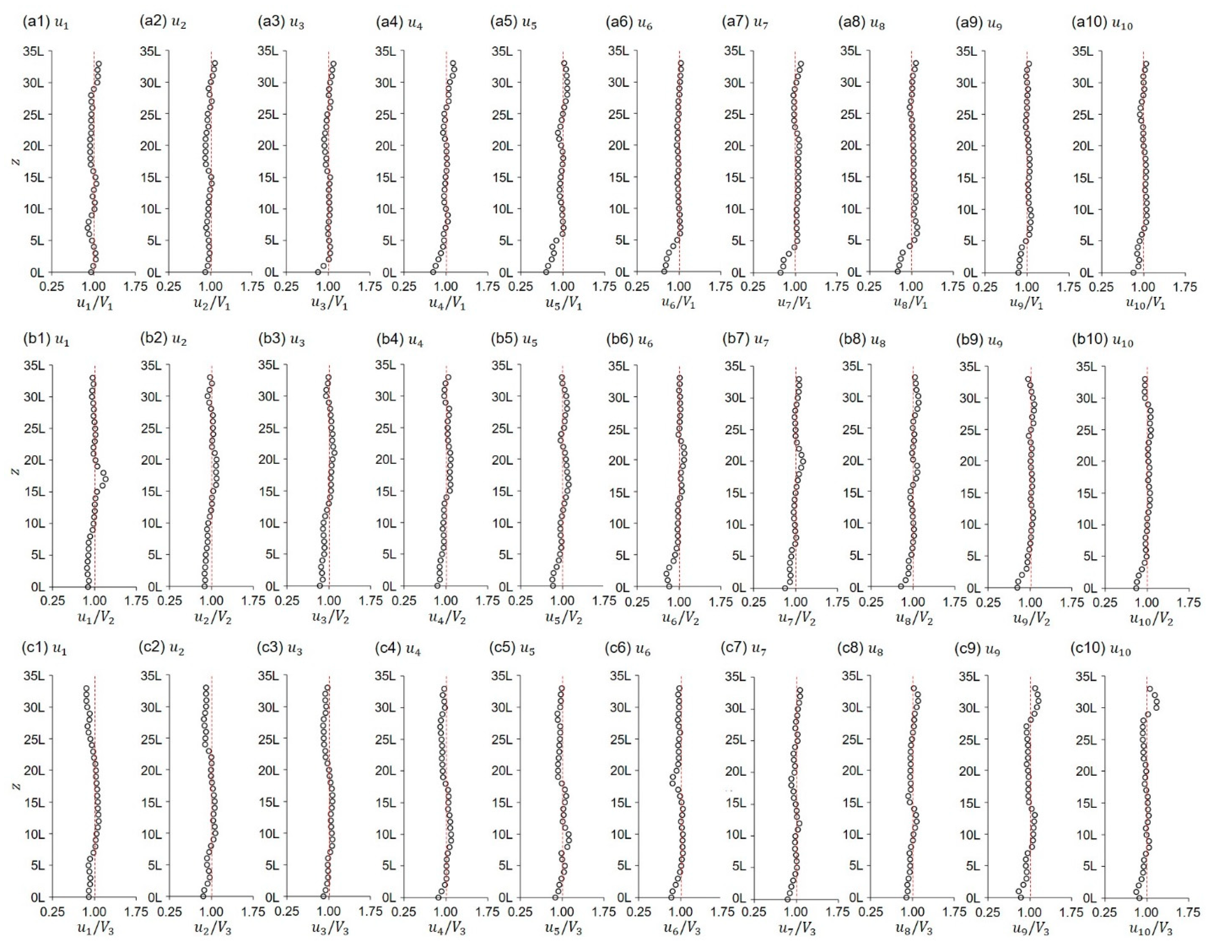
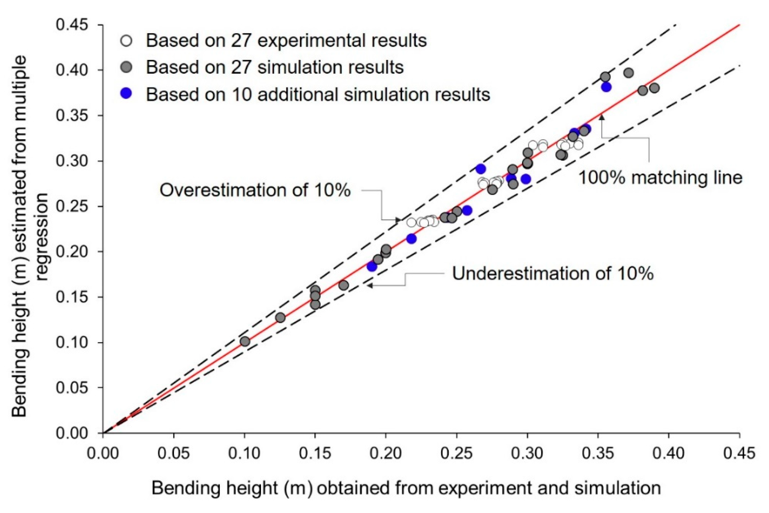
3.2. Regression Analysis

We performed 27 additional simulations (

Table 5. Bending height of vegetation estimated by the FSI simulation considering 27 additionally designed simulation cases.

Case	Density (kg m−3)	Young’s Modulus (Pa)	Vegetation Height (m)	Width (m)	Thickness (m)	Inlet Velocity (m s−1)	Bending Height (m)
Sim_01	1500	3.00 × 109	0.275	0.020	0.002	0.100	0.275
Sim_02	2000	2.00 × 109	0.325	0.015	0.002	0.050	0.325
Sim_03	500	1.00 × 109	0.150	0.030	0.003	0.200	0.150
Sim_04	2500	5.00 × 108	0.200	0.040	0.002	0.150	0.200
Sim_05	3000	1.50 × 109	0.175	0.005	0.001	0.250	0.170
Sim_06	3500	5.00 × 109	0.300	0.050	0.005	0.300	0.300
Sim_07	4000	3.00 × 109	0.400	0.040	0.003	0.400	0.389
Sim_08	4500	7.00 × 109	0.250	0.030	0.002	0.250	0.250
Sim_09	5000	2.00 × 109	0.450	0.010	0.001	0.175	0.355
Sim_10	2200	1.80 × 109	0.300	0.030	0.003	0.200	0.300
Sim_11	1000	1.20 × 109	0.200	0.020	0.003	0.300	0.200
Sim_12	3000	2.50 × 109	0.300	0.020	0.003	0.100	0.300
Sim_13	1750	3.00 × 109	0.350	0.030	0.002	0.250	0.340
Sim_14	2250	1.75 × 109	0.250	0.025	0.002	0.300	0.241
Sim_15	3000	2.50 × 109	0.150	0.005	0.001	0.200	0.150
Sim_16	3500	1.00 × 109	0.325	0.015	0.002	0.150	0.323
Sim_17	1000	2.00 × 109	0.125	0.010	0.002	0.250	0.125
Sim_18	2000	7.50 × 108	0.300	0.030	0.003	0.100	0.300
Sim_19	1500	5.00 × 108	0.150	0.020	0.002	0.200	0.150
Sim_20	4000	2.00 × 109	0.250	0.025	0.002	0.300	0.246
Sim_21	2500	3.00 × 109	0.300	0.010	0.003	0.400	0.290
Sim_22	2750	2.50 × 109	0.350	0.010	0.002	0.250	0.332
Sim_23	3750	5.00 × 109	0.400	0.030	0.002	0.175	0.381
Sim_24	750	1.25 × 109	0.200	0.040	0.001	0.200	0.194
Sim_25	1750	3.25 × 109	0.300	0.020	0.001	0.225	0.290
Sim_26	2250	4.00 × 109	0.100	0.010	0.002	0.325	0.100
Sim_27	1000	2.25 × 109	0.450	0.010	0.001	0.150	0.371

) to create a large dataset for multiple regression analysis; we considered the densities, Young’s moduli, geometrical properties, and flow velocities of previous studies (Table 1). Of the 27 additional results, 15 exhibited rather small horizontal deformations attributable to the chosen densities, Young’s moduli, vegetation heights, second moments of cross-sectional areas, and flow velocities; the bending heights were nearly identical to the vegetation heights. These data were used for multiple regression analysis, as were the 27 experimental data (Table 4).

We considered vegetation height ($h_v$), vegetation thickness ($t_v$), vegetation width ($w_v$), vegetation density (${\rho }_v$), Young’s modulus ($E_v$), and water velocity ($V$) as independent variables in the regression analysis because the bending behavior of a long and slender vegetation correlates with cross-sectional area, stiffness, and external force.

We applied the Buckingham Π theorem [53,54] to find the relationship of the bending height with the relevant variables. First, we considered the bending height ($h_b$) of vegetation as a function of the six independent variables, as shown in Equation (8):

$$h_b=f\left(h_v, t_v,w_v,{\rho }_v,E_v,V\right).$$

(8)

We carried out the factor analysis to understand the complex relationship among the six independent variables. As a result, we identified the latent factors as follows: (a) vegetation height ($h_v$) and width ($w_v$) representing the cross-section property of the vegetation stem; (b) water velocity ($V$) and vegetation density (${\rho }_v$) representing the external force; and (c) vegetation height ($h_v$) and Young’s modulus ($E_v$) representing the stiffness.

The dimensions of those seven variables, including $h_b$, are the combinations of M (mass), L (length), and T (time), which are represented by the units of kilogram (kg), meter (m), and second (s), respectively. According to the three fundamental dimensions and seven variables, we considered four non-dimensional parameters, i.e., ${\pi }_i$ ($i$ = 1, 2, 3, and 4). Of those variables, we selected $E_v$, $V$, and $h_v$ as the repeating variables as these present the material property, flow property, and geometric property, respectively. Then, we took the remaining variables along with these variables one by one to create the non-dimensional groups. The first non-dimensional group is shown in Equation (9a):

$${\pi }_1=h_b{\left(E_v\right)}^a{\left(h_v\right)}^b{\left(V\right)}^c\equiv {\mathrm{L}}^{1-a+b+c}{\mathrm{M}}^a{\mathrm{T}}^{-2a-c}.$$

(9a)

To make Equation (9a) dimensionless, we selected $a=c=0$ and $b=-1$; hence, Equation (9a) becomes Equation (9b):

$${\pi }_1=h_b/h_v.$$

(9b)

Similarly, we obtained Equations (10) and (11) for the second and third non-dimensional groups, respectively:

$${\pi }_2=w_v{\left(E_v\right)}^a{\left(h_v\right)}^b{\left(V\right)}^c\equiv {\mathrm{L}}^{1-a+b+c}{\mathrm{M}}^a{\mathrm{T}}^{-2a-c}$$

(10a)

$${\pi }_2=w_v/h_v$$

(10b)

$${\pi }_3=t_v{\left(E_v\right)}^a{\left(h_v\right)}^b{\left(V\right)}^c\equiv {\mathrm{L}}^{1-a+b+c}{\mathrm{M}}^a{\mathrm{T}}^{-2a-c}$$

(11a)

$${\pi }_3=t_v/h_v.$$

(11b)

The fourth non-dimensional group is shown in Equation (12a), and by selecting $a=-1$, $b=0$, and $c=2$, its dimensionless form becomes Equation (12b).

$${\pi }_4={\rho }_v{\left(E_v\right)}^a{\left(h_v\right)}^b{\left(V\right)}^c\equiv {\mathrm{L}}^{-3-a+b+c}{\mathrm{M}}^{1+a}{\mathrm{T}}^{-2a-c}$$

(12a)

$${\pi }_4={\rho }_v{V}^2/E_v$$

(12b)

According to the four non-dimensional parameters ${\pi }_1=h_b/h_v$, ${\pi }_2=w_v/h_v$, ${\pi }_3=t_v/h_v$, and ${\pi }_4={\rho }_v{V}^2/E_v$, we can establish Equation (13):

$${\pi }_1=f\left({\pi }_2,{\pi }_3,{\pi }_4\right)\mathrm{or}\frac{h_b}{h_v}=f\left(\frac{w_v}{h_v},\frac{t_v}{h_v},\frac{{\rho }_v{V}^2}{E_v}\right).$$

(13)

Considering Equation (13), we can obtain Equations (14a) and (14b):

$$\frac{h_b}{h_v}={\beta }_0{\left(\frac{w_v}{h_v}\right)}^{{\beta }_1}{\left(\frac{t_v}{h_v}\right)}^{{\beta }_2}{\left(\frac{{\rho }_v{V}^2}{E_v}\right)}^{{\beta }_3}$$

(14a)

$$\ln \left(\frac{h_b}{h_v}\right)=\ln {\beta }_0+{\beta }_1\ln \left(\frac{w_v}{h_v}\right)+{\beta }_2\ln \left(\frac{t_v}{h_v}\right)+{\beta }_3\ln \left(\frac{{\rho }_v{V}^2}{E_v}\right).$$

(14b)

We used the experimental and simulation data to derive the coefficients ${\beta }_0=$ 1.2831, ${\beta }_1=$ 0.0145, ${\beta }_2=$ 0.0676, and ${\beta }_3=-$0.0051; hence, the regression equation is determined as Equation (15):

$$h_b=1.2831h_v{\left(\frac{w_v}{h_v}\right)}^{0.0145}{\left(\frac{t_v}{h_v}\right)}^{0.0676}{\left(\frac{{\rho }_v{V}^2}{E_v}\right)}^{-0.0051}$$

(15)

In Figure 8, the white and gray circles are the bending heights from multiple regression analysis of the 27 experimental data (Table 4) and 27 simulation data (Table 5), respectively. Most circles are within the 10% overestimation and underestimation lines and thus close to the 100% matching line; the multiple regression results were in good agreement with the experimental and simulation results. To further verify the accuracy of the regression analysis, the FSI simulation and multiple regression equation were used to calculate the bending heights for a further ten cases (blue circles in Figure 8). All blue circles are within the 10% lines and thus close to the 100% matching line, further validating the accuracy of the regression analysis.

Figure 9 shows the relative % errors of the bending heights predicted from the multiple regression equation using the 27 experimental results, the 27 simulations, and the 10 additional simulations. Of the 64 cases, 63 had errors < 10%, and 1 had an error of 10.71%. Thus, the multiple regression equation adequately estimated bending heights using the vegetation density, Young’s modulus, the vegetation height, width, thickness, and the water flow velocity.

Figure 10 compares the ratio $\left(h_b/h_v\right)$ of the present study with those of Fonseca and Kenworthy [32], Luhar and Nepf [30], and Zeller et al. [33]. The data from Fonseca and Kenworthy [32], denoted by FK87 in the figure, were derived from a lab-scale experiment involving live vegetation exposed to unidirectional flow. The results from Luhar and Nepf [30], denoted by LN11, were obtained from a theoretical model predicting the bending height of a single artificial flexible vegetation stem under unidirectional flow. The data from Zeller et al. [33], denoted by Z14, were obtained from a lab-scale experiment using a blade model exposed to both wave and current conditions.

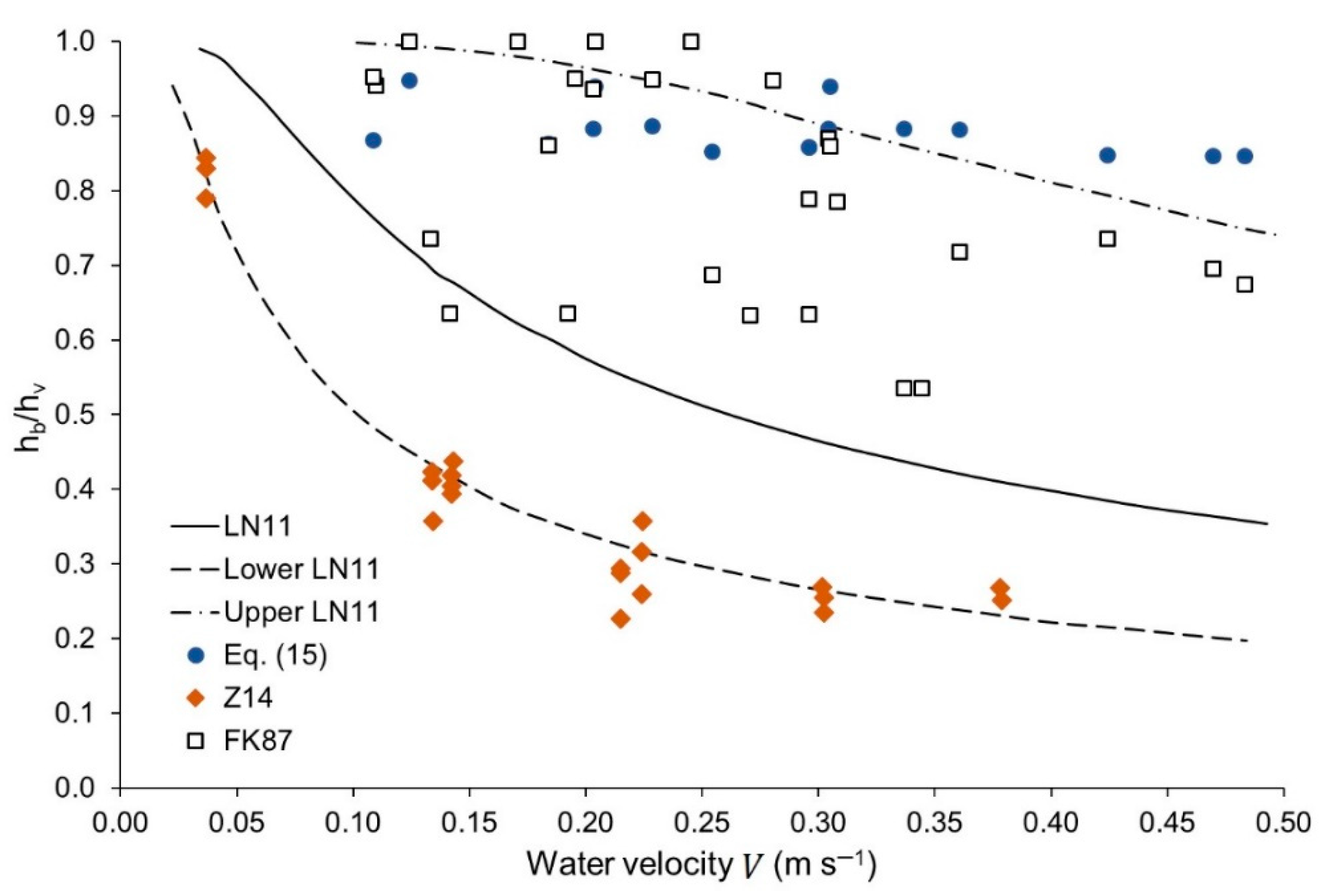
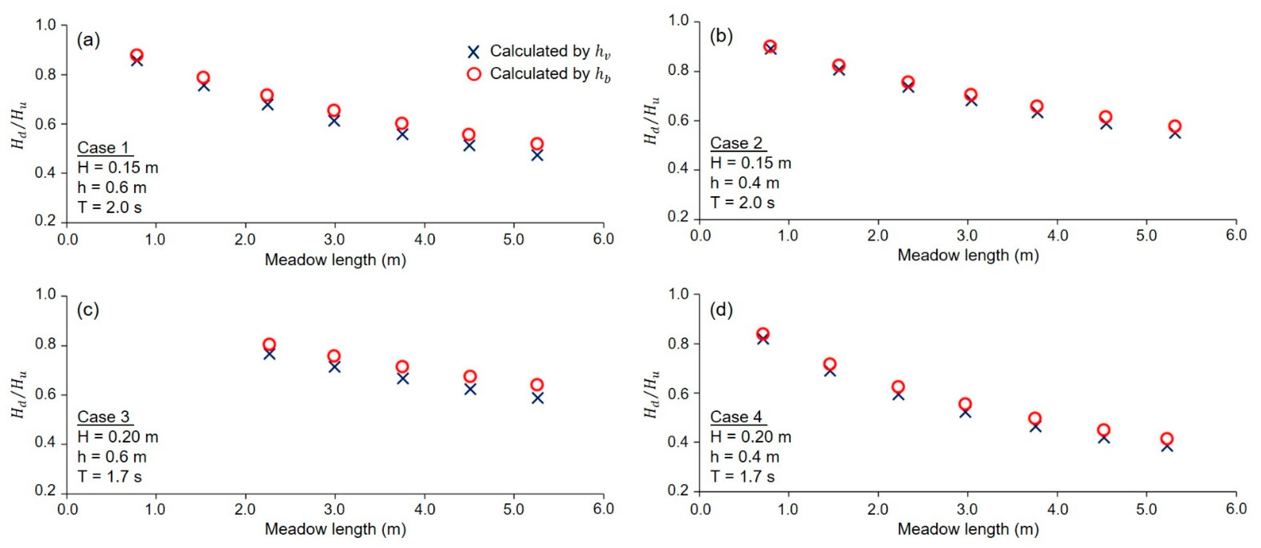
3.3. Effect of Bending Behavior on Wave Height

Most studies focused on wave attenuation solely through wave forces, overlooking the impact of currents. However, the presence of currents significantly diminishes the wave attenuation capacity, particularly in scenarios involving flexible vegetation [36,55]. Currents induce vegetation bending, while waves induce swaying [31,56]. Currents cause vegetation to move, reducing the front area perpendicular to the flow, lowering drag and reducing wave attenuation [30,31]. Thus, to account for the effect of bending behavior on wave height, we estimated the reduction in front area of vegetation and wave attenuation. To quantify the significance of this effect, we considered the experiment conducted by Losada et al. [31]. They used live vegetation (Puccinellia maritima), specified by Young’s modulus of stems (13 MPa), Young’s modulus of leaves (7.8 MPa), stem height (0.473 m), leaf height (0.230 m), number of leaves per stem (5.5), leaf width (0.003 m), and shoot density (2436). The water and wave properties [31] considered are shown in

Table 6. Water flow properties [31] considered.

Case	Wave Height H (m)	Water Depth h (m)	Wave Period T (s)	Current Velocity V (m s−1)
1	0.15	0.60	2.00	0.30
2	0.15	0.40	2.00	0.30
3	0.20	0.60	1.70	0.30
4	0.20	0.40	1.70	0.30

.

To calculate the wave height, Losada et al. [31] developed Equation (16) based on linear wave theory and energy conservation:

$$\frac{H\left(x\right)}{H_u}=\frac{1}{1+\beta x}$$

(16)

where $H\left(x\right)$ is the downstream wave height measured at $\mathrm{a}\mathrm{distance} x$ (unit: m) away from the forefront of the vegetation meadow, and is $\beta$ a damping factor. The damping factor is shown in Equation (17), which is a function of wave height at upstream $H_u$ and two coefficients $A_0$ (Equation (18)) and $B$ (Equation (19)):

$$\beta =\frac{A_0{H}_u}{B}$$

(17)

$$A_0=\frac{2}{3\pi }\rho C_d{w}_{v}N{\left(\frac{gk}{2\left(\omega -Vk\right)}\right)}^3\frac{{\sin \mathrm{h}}^{3}k{h}_v+3\sin \mathrm{h}k{h}_v}{3k{\cos \mathrm{h}}^{3}kh}$$

(18)

$$\begin{array}{ll}B=& [\frac{\rho g}{8}\left(1+\frac{2kh}{\sin \mathrm{h}2kh}\right){\left(\frac{g}{k}\tan \mathrm{h}kh\right)}^{1/2}+\frac{\rho g}{8}V\left(3+\frac{4kh}{\sin \mathrm{h}2kh}\right)\\ & +\frac{3\rho k}{8}{V}^2{\left(\frac{g}{k}\cot \mathrm{h}kh\right)}^{1/2}]\left[V+\frac{1}{2}\left(1+\frac{2kh}{\sin \mathrm{h}2kh}\right){\left(\frac{g}{k}\tan \mathrm{h}kh\right)}^{1/2}\right]\end{array}$$

(19)

Equation (20) shows the dispersion relation for the wave number $k$:

$$\frac{4{\pi }^2}{g{T}^2}h=kh\tanh kh$$

(20)

where $C_d$ is the drag coefficient, $N$ the shoot density, $\omega$ the angular frequency, and $h$ the water depth. By using the damping factor provided by Losada et al. [31], we estimated $C_d$ from Equations (17)–(19). Then, the wave height downstream was calculated by Equation (16). Finally, the effect of bending behavior could be explored by Equation (21):

$$\alpha =\frac{H_{d\_v}-H_{d\_b}}{H_{d\_v}}\times 100\%$$

(21)

where $\alpha$ is the relative % decrease in wave height reduction considering the wave heights downstream from $H_{d\_b}$ and $H_{d\_v}$ due to the bending height $h_b$ and vegetation height $h_v$, respectively.

Figure 11 shows the ratios of downstream wave heights and upstream wave heights ($H_d/H_u$) obtained in this study; the corresponding meadow lengths are 0.79–5.26 m for case 1, 0.80–5.32 m for case 2, 2.27–5.26 m for case 3, and 0.72–5.23 m for case 4. From the figure, we can observe that the $H_d/H_u$ ratios calculated by $h_b$ appear larger than those calculated by $h_v$ for the four cases. This indicates that the wave height is reduced less when bending behavior is taken into account. This is because the bending behavior of vegetation reduces the frontal area, consequently reducing the energy lost in a wave travelling over vegetation [34,57]. Therefore, calculating the wave height from the bending height decreases the wave height reduction compared with calculating it from the vegetation height. As the experiment of Losada et al. [31] pointed out, vegetation stems bend in the flow direction; hence, utilizing the bending height for wave height calculation reflects the actual motion of the vegetation stem, unlike when using the vegetation height.

4. Discussion

Luhar and Nepf [30] considered relatively extensive vegetation properties, including width (1 cm), thickness (0.45 mm), height (10 cm to 30 cm), and elastic modulus (0.4 GPa to 2.4 GPa). Thus, their results (three lines in Figure 10) correspond to the maximum (dot-solid line; upper LN11), minimum (dotted line; lower LN11), and middle values (solid line; LN11) of $h_b/h_v$, respectively. The experimental results of Z14 are near the lower limit of LN11. This is because Zeller et al. [33] used an elastic modulus of 0.3 GPa for a single artificial vegetation blade. In contrast, FK87 reached the upper limit of LN11. This is because the vegetation stems caused a decrease in velocity inside the meadow, leading to increased bending height, and the elastic modulus of live vegetation was relatively high in the work of Fonseca and Kenworthy [32]. This point was also discussed by Luhar and Nepf [30]. The regression equation, Equation (15), was derived from data with an elastic modulus of 0.5 GPa to 7.5 GPa, which is close to the upper limit data (2.4 GPa) of Luhar and Nepf [30]; hence, our results were also close to the upper limit.

As the vegetation meadow increases, the relative % decrease in wave height reduction ($\alpha$) increases linearly, up to ~10% (9.23%) in the selected case studies (Figure 12). This implies that the impact of bending behavior becomes more pronounced with a larger vegetation meadow. In the figure, $\alpha$ is greater when the water depth is 0.60 m compared to 0.40 m. Considering the vegetation height of 0.588 m in our calculation, this indicates that the vegetation is fully submerged at a water depth of 0.60 m but partially submerged at 0.40 m; hence, $\alpha$ is greater in a fully submerged vegetation meadow than in a partially submerged vegetation meadow. In a fully submerged meadow, the current acts along the entire stem height, resulting in greater deformation or a smaller bending height.

Calculating the wave height reduction using the vegetation height (assuming no bending occurs) implicitly implies that the vegetation is rigid. In contrast, when bending occurs, the vegetation can be considered flexible. Therefore, our results also indicate that rigid vegetation can reduce wave height ~10% more effectively than flexible vegetation. This argument aligns with the findings of other studies. For example, van Veelen et al. [34] reported that flexible vegetation attenuated waves by up to 70% less than rigid vegetation because flexible plants swayed, reducing the frontal area, the total work performed by the drag force, and thus the total wave energy lost when traveling over vegetation. Liu et al. [58] also noted that rigid vegetation was more effective in reducing wave heights compared to flexible vegetation in their laboratory-scale study. However, they did not specify the extent of such a reduction. Moreover, Mullarney and Henderson [59] found in field experiments that wave dissipation increased with the stiffness of vegetation stems. The overall wave dissipation in the flexible stems was approximately 30% of that observed in the rigid stems.

The work had certain limitations. First, we considered only a single type of vegetation and assumed that all vegetation stems bent identically in water flow. Vegetation on the front of a meadow is more likely to bend than vegetation behind the front; hence, this assumption may yield overestimates of the extents to which vegetation meadows reduce wave height. Second, during the FSI simulation, the water velocity was assumed to be uniform and temporally independent. In other words, the velocity remained constant throughout the vegetation meadow during the simulation. Third, although vegetation both bends and sways in water flow, we only focused on bending.

5. Conclusions

We considered nine types of marine vegetation and three water velocities, constructed 27 experimental cases, and obtained the bending heights via PIV measurements and FSI simulations. Of the 27 simulation results, 24 had errors < 5% in the experimental results; thus, the simulation was reliable. An additional 27 simulations were performed to provide a large dataset for multi-regression analysis (54 cases). To further validate the regression equation, an additional ten cases were considered. As a result, 63 of the 64 cases had errors < 10%, and 1 had an error of 10.71%. Moreover, a reasonable comparative result was achieved when we compared our regression equation with the existing lab-scale experiments and theoretical solutions. Thus, the multiple regression equation simply estimated the bending height with a tolerance of ~10%, showing the effectiveness of calibrating the vegetation height due to bending behavior. Based on these estimations, we predicted the effect of bending behavior on wave height. First, flexible vegetation was found to be up to ~10% less effective in reducing wave height than rigid vegetation. This is because bending reduced the frontal area of vegetation, the total work performed by the drag force, and the total energy lost by a wave traveling over the vegetation meadow. Second, the relative % decrease in wave height reduction increased as the vegetation meadow size increased, ranging from 1.08% to 9.23% in our investigation, particularly with a vegetation meadow of approximately 5 m. This implies that the impact of bending behavior becomes more pronounced with a larger vegetation meadow. Finally, we observed that the relative % decrease in wave height reduction was greater for fully submerged vegetation compared to partially submerged vegetation.

References

1. Ghaderpour, E.; Abbes, A.B.; Rhif, M.; Pagiatakis, S.D.; Farah, I.R. Non-stationary and unequally spaced NDVI time series analyses by the LSWAVE software. Int. J. Remote Sens. 2020, 41, 2374–2390. [Google Scholar] [CrossRef]
2. He, Y.; Lee, E. Empirical relationships of sea surface temperature and vegetation activity with summer rainfall variability over the Sahel. Earth Interact. 2016, 20, 1–18. [Google Scholar] [CrossRef]
3. Oliver, E.C.J.; Donat, M.G.; Burrows, M.T.; Moore, P.J.; Smale, D.A.; Alexander, L.V.; Benthuysen, J.A.; Feng, M.; Gupta, A.S.; Hobday, A.J.; et al. Longer and more frequent marine heatwaves over the past century. Nat. Commun. 2018, 9, 1324. [Google Scholar] [CrossRef]
4. Jung, S.; Chau, V.T.; Kim, M.; Na, W.B. Artificial seaweed reefs that support the establishment of submerged aquatic vegetation beds and facilitate ocean macroalgal afforestation: A review. J. Mar. Sci. Eng. 2022, 10, 1184. [Google Scholar] [CrossRef]
5. Barahimi, M.; Sui, J. Effects of submerged vegetation arrangement patterns and density on flow structure. Water 2023, 15, 176. [Google Scholar] [CrossRef]
6. Box, W.; Järvelä, J.; Västilä, K. Flow resistance of floodplain vegetation mixtures for modelling river flows. J. Hydrol. 2021, 601, 126593. [Google Scholar] [CrossRef]
7. Stocker, B.D.; Tumber-Dávila, S.J.; Konings, A.G.; Anderson, M.C.; Hain, C.; Jackson, R.B. Global patterns of water storage in the rooting zones of vegetation. Nat. Geosci. 2023, 16, 250–256. [Google Scholar] [CrossRef] [PubMed]
8. Tang, C.; Liu, Y.; Li, Z.; Guo, L.; Xu, A.; Zhao, J. Effectiveness of vegetation cover pattern on regulating soil erosion and runoff generation in red soil environment, southern China. Ecol. Indic. 2021, 129, 107956. [Google Scholar] [CrossRef]
9. Bai, G.; Xu, D.; Zou, Y.; Liu, Y.; Liu, Z.; Luo, F.; Wang, C.; Zhang, C.; Liu, B.; Zhou, Q.; et al. Impact of submerged vegetation, water flow field and season changes on sediment phosphorus distribution in a typical subtropical shallow urban lake: Water nutrients state determines its retention and release mechanism. J. Environ. Chem. Eng. 2022, 10, 107982. [Google Scholar] [CrossRef]
10. Clarke, S.J. Vegetation growth in rivers: Influences upon sediment and nutrient dynamics. Prog. Phys. Geog. 2002, 26, 159–172. [Google Scholar] [CrossRef]
11. Toromanovic, M.; Ibrahimpašić, J.; Topalić-Trivunović, L.; Šišić, I. Removal of organic pollutants from municipal wastewater by a horizontal pilot-scale constructed wetland utilizing Phragmites australis and Typha latifolia–Effectiveness monitoring per season. J. Chem. Technol. Environ. 2018, 10, 39–44. [Google Scholar] [CrossRef]
12. Wang, C.; Zheng, S.S.; Wang, P.F.; Qian, J. Effects of vegetations on the removal of contaminants in aquatic environments: A review. J. Hydrodyn. 2014, 26, 497–511. [Google Scholar] [CrossRef]
13. John, B.M.; Shirlal, K.G.; Rao, S. Effect of artificial sea grass on wave attenuation- an experimental investigation. Aquat. Procedia 2015, 4, 221–226. [Google Scholar] [CrossRef]
14. Morris, R.L.; Graham, T.D.J.; Kelvin, J.; Ghisalberti, M.; Swearer, S.E. Kelp beds as coastal protection: Wave attenuation of Ecklonia radiata in a shallow coastal bay. Ann. Bot. 2020, 125, 235–246. [Google Scholar] [CrossRef]
15. Sánchez-González, J.F.; Sánchez-Rojas, V.; Memos, C.D. Wave attenuation due to Posidonia oceanica meadows. J. Hydraul. Res. 2011, 49, 503–514. [Google Scholar] [CrossRef]
16. Sigren, J.M.; Figlus, J.; Armitage, A.R. Coastal sand dunes and dune vegetation: Restoration, erosion, and storm protection. Shore Beach 2014, 82, 5–12. [Google Scholar]
17. Manousakas, N.; Salauddin, M.; Pearson, J.; Denissenko, P.; Williams, H.; Abolfathi, S. Effects of seagrass vegetation on wave runup reduction—A laboratory study. IOP Conf. Ser. Earth Environ. Sci. 2022, 1072, 012004. [Google Scholar] [CrossRef]
18. Augustin, L.N.; Irish, J.L.; Lynett, P. Laboratory and numerical studies of wave damping by emergent and near-emergent wetland vegetation. Coast. Eng. 2009, 56, 332–340. [Google Scholar] [CrossRef]
19. Koftis, T.; Prinos, P.; Stratigaki, V. Wave damping over artificial Posidonia oceanica meadow: A large-scale experimental study. Coast. Eng. 2013, 73, 71–83. [Google Scholar] [CrossRef]
20. Stratigaki, V.; Manca, E.; Prinos, P.; Losada, I.J.; Lara, J.L.; Sclavo, M.; Amos, C.L.; Cáceres, I.; Sánchez-Arcilla, A. Large-scale experiments on wave propagation over Posidonia oceanica. J. Hydraul. Res. 2011, 49, 31–43. [Google Scholar] [CrossRef]
21. Cao, H.; Chen, Y.; Tian, Y.; Feng, W. Field investigation into wave attenuation in the mangrove environment of the South China Sea coast. J. Coastal Res. 2016, 32, 1417–1427. [Google Scholar] [CrossRef]
22. Nowacki, D.J.; Beudin, A.; Ganju, N.K. Spectral wave dissipation by submerged aquatic vegetation in a back-barrier estuary. Limnol. Oceanogr. 2017, 62, 736–753. [Google Scholar] [CrossRef]
23. Paquier, A.E.; Oudart, T.; Le Bouteiller, C.; Meulé, S.; Larroudé, P.; Dalrymple, R.A. 3D numerical simulation of seagrass movement under waves and currents with GPUSPH. Int. J. Sediment Res. 2021, 36, 711–722. [Google Scholar] [CrossRef]
24. Yin, K.; Xu, S.; Huang, W.; Liu, S.; Li, M. Numerical investigation of wave attenuation by coupled flexible vegetation dynamic model and XBeach wave model. Ocean Eng. 2021, 235, 109357. [Google Scholar] [CrossRef]
25. Twomey, A.J.; O’Brien, K.R.; Callaghan, D.P.; Saunders, M.I. Synthesising wave attenuation for seagrass: Drag coefficient as a unifying indicator. Mar. Pollut. Bull. 2020, 160, 111661. [Google Scholar] [CrossRef]
26. Fonseca, M.S.; Cahalan, J.A. A preliminary evaluation of wave attenuation by four species of seagrass. Estuar. Coast. Shelf Sci. 1992, 35, 565–576. [Google Scholar] [CrossRef]
27. Yiping, L.; Anim, D.O.; Wang, Y.; Tang, C.; Du, W.; Lixiao, N.; Yu, Z.; Acharya, K.; Chen, L. Laboratory simulations of wave attenuation by an emergent vegetation of artificial Phragmites australis: An experimental study of an open-channel wave flume. J. Environ. Eng. Landsc. Manag. 2015, 23, 251–266. [Google Scholar] [CrossRef]
28. Hashim, A.M.; Catherine, S.M.P. A Laboratory study on wave reduction by mangrove forests. APCBEE Procedia 2013, 5, 27–32. [Google Scholar] [CrossRef]
29. He, F.; Chen, J.; Jiang, C. Surface wave attenuation by vegetation with the stem, root and canopy. Coast. Eng. 2019, 152, 103509. [Google Scholar] [CrossRef]
30. Luhar, M.; Nepf, H.M. Flow-induced reconfiguration of buoyant and flexible aquatic vegetation. Limnol. Oceanogr. 2011, 56, 2003–2017. [Google Scholar] [CrossRef]
31. Losada, I.J.; Maza, M.; Lara, J.L. A new formulation for vegetation-induced damping under combined waves and currents. Coast. Eng. 2016, 107, 1–13. [Google Scholar] [CrossRef]
32. Fonseca, M.S.; Kenworthy, W.J. Effects of current on photosynthesis and distribution of seagrasses. Aquat. Bot. 1987, 27, 59–78. [Google Scholar] [CrossRef]
33. Zeller, R.B.; Weitzman, J.S.; Abbett, M.E.; Zarama, F.J.; Fringer, O.B.; Koseff, J.R. Improved parameterization of seagrass blade dynamics and wave attenuation based on numerical and laboratory experiments. Limnol. Oceanogr. 2014, 59, 251–266. [Google Scholar] [CrossRef]
34. van Veelen, T.J.; Fairchild, T.P.; Reeve, D.E.; Karunarathna, H. Experimental study on vegetation flexibility as control parameter for wave damping and velocity structure. Coast. Eng. 2020, 157, 103648. [Google Scholar] [CrossRef]
35. Folkard, A.M. Hydrodynamics of model Posidonia oceanica patches in shallow water. Limnol. Oceanogr. 2005, 50, 1592–1600. [Google Scholar] [CrossRef]
36. Paul, M.; Bouma, T.J.; Amos, C.L. Wave attenuation by submerged vegetation: Combining the effect of organism traits and tidal current. Mar. Ecol. Prog. Ser. 2012, 444, 31–41. [Google Scholar] [CrossRef]
37. Weitzman, J.S.; Zeller, R.B.; Thomas, F.I.M.; Koseff, J.R. The attenuation of current- and wave-driven flow within submerged multispecific vegetative canopies. Limnol. Oceanogr. 2015, 60, 1855–1874. [Google Scholar] [CrossRef]
38. Atkins, M.D. Chapter 5–velocity field measurement using particle image velocimetry (PIV). In Application of Thermo-Fluidic Measurement Techniques: An Introduction; Kim, T., Lu, T.J., Song, S.J., Eds.; Butterworth-Heinemann: Cambridge, MA, USA, 2016; pp. 125–166. ISBN 978-012-809-731-1. [Google Scholar]
39. Lee, Y.J.; Jung, S.; Na, W.B. Estimating movement and falling distances of underwater free-falling cuboid models for marine habitat enhancement structures considering horizontal water flow. Ocean Eng. 2022, 262, 112172. [Google Scholar] [CrossRef]
40. Pauls, J.P.; Bartnikowski, N.; Jansen, S.H.; Lim, E.; Dasse, K. Chapter 13–Preclinical evaluation. In Mechanical Circulatory and Respiratory Support; Gregory, S.D., Stevens, M.C., Fraser, J.F., Eds.; Academic Press: Cambridge, MA, USA, 2018; pp. 407–438. ISBN 978-012-810-491-0. [Google Scholar]
41. Chen, S.N.; Sanford, L.P.; Koch, E.W.; Shi, F.; North, E.W. A nearshore model to investigate the effects of seagrass bed geometry on wave attenuation and suspended sediment transport. Estuar. Coast. 2007, 30, 296–310. [Google Scholar] [CrossRef]
42. Axisa, F.; Antunes, J. Modelling of Mechanical Systems: Fluid Structure Interaction; Butterworth-Heinemann: Jordan Hill, Oxford, UK, 2007; pp. 1–44. ISBN 978-075-066-847-7. [Google Scholar]
43. Lee, K.; Huque, Z.; Kommalapati, R.; Han, S.E. The evaluation of aerodynamic interaction of wind blade using fluid structure interaction method. J. Clean Energy Technol. 2015, 3, 270–275. [Google Scholar] [CrossRef]
44. El Maani, R.; Radi, B.; El Hami, A. Vibratory reliability analysis of an aircraft’s wing via fluid-structure interactions. Aerospace 2017, 4, 40. [Google Scholar] [CrossRef]
45. Hirschhorn, M.; Tchantchaleishvili, V.; Stevens, R.; Rossano, J.; Throckmorton, A. Fluid–structure interaction modeling in cardiovascular medicine—A systematic review 2017–2019. Med. Eng. Phys. 2020, 78, 1–13. [Google Scholar] [CrossRef] [PubMed]
46. Kamakoti, R.; Shyy, W. Fluid-structure interaction for aeroelastic applications. Prog. Aerosp. Sci. 2004, 40, 535–558. [Google Scholar] [CrossRef]
47. Sederstrom, D.R. Methods and Implementation of Fluid-Structure Interaction Modeling into an Industry-Accepted Design Tool. Ph.D. Thesis, University of Denver, Denver, FL, USA, 2016; pp. 1–30. [Google Scholar]
48. Kim, D.; Jung, S.; Na, W.B. Evaluation of turbulence models for estimating the wake region of artificial reefs using particle image velocimetry and computational fluid dynamics. Ocean Eng. 2021, 223, 108673. [Google Scholar] [CrossRef]
49. ANSYS Inc. ANSYS Fluent User’s Guide Release 2020 R1; ANSYS Inc.: Canonsburg, PA, USA, 2020. [Google Scholar]
50. Tadepalli, S.C.; Erdemir, A.; Cavanagh, P.R. Comparison of hexahedral and tetrahedral elements in finite element analysis of the foot and footwear. J. Biomech. 2011, 44, 2337–2343. [Google Scholar] [CrossRef] [PubMed]
51. ANSYS Inc. ANSYS Fluent Theory Guide Release 2020 R1; ANSYS Inc.: Canonsburg, PA, USA, 2020. [Google Scholar]
52. Drevon, D.; Fursa, S.R.; Malcolm, A.L. Intercoder reliability and validity of WebPlotDigitizer in extracting graphed data. Behav. Modif. 2016, 41, 323–339. [Google Scholar] [CrossRef] [PubMed]
53. Buckingham, E. The principle of similitude. Nature 1915, 96, 396–397. [Google Scholar] [CrossRef]
54. Dumka, P.; Chauhan, R.; Singh, A.; Singh, G.; Mishra, D. Implementation of Buckingham’s Pi theorem using Python. Adv. Eng. Softw. 2022, 173, 103232. [Google Scholar] [CrossRef]
55. Maza, M.; Lara, J.L.; Losada, I.J.; Ondiviela, B.; Trinogga, J.; Bouma, T.J. Large-scale 3-D experiments of wave and current interaction with real vegetation. Part 2: Experimental analysis. Coast. Eng. 2015, 106, 73–86. [Google Scholar] [CrossRef]
56. Henderson, S.M. Motion of buoyant, flexible aquatic vegetation under waves: Simple theoretical models and parameterization of wave dissipation. Coast. Eng. 2019, 152, 103497. [Google Scholar] [CrossRef]
57. Dalrymple, R.A.; Kirby, J.T.; Hwang, P.A. Wave diffraction due to areas of energy dissipation. J. Waterw. Port Coast. Ocean Eng. 1984, 110, 67–79. [Google Scholar] [CrossRef]
58. Liu, S.; Xu, S.; Yin, K. Optimization of the drag coefficient in wave attenuation by submerged rigid and flexible vegetation based on experimental and numerical studies. Ocean Eng. 2023, 285, 115382. [Google Scholar] [CrossRef]
59. Mullarney, J.C.; Henderson, S.M. Wave-forced motion of submerged single-stem vegetation. J. Geophys. Res. Oceans 2010, 115, C12061. [Google Scholar] [CrossRef]
Figure 1. PIV experimental setup.
Jmse 12 01054 g001
Figure 2. Mapping region for capturing a velocity profile: (a) 10 locations (0 L–27 L) vertically divided and 12 locations (0 L–33 L) horizontally divided, where L = 10.765 mm, and (b) window (~290 mm × 355 mm) for measuring water velocity, showing the instantaneous velocity vector field obtained from the PIV measurement.
Jmse 12 01054 g002
Figure 3. Independence tests for (a) domain length, (b) number of iteration steps, (c) analysis time, and (d) number of elements. Here, the relative % errors are with respect to the selected point; those errors, by definition, must all be positive; however, the “–” sign was intentionally added to highlight the differences with respect to the reference values.
Jmse 12 01054 g003
Figure 4. Domain, boundary conditions, and mesh configuration: (a) domain and boundary conditions and (b) mesh configuration.
Jmse 12 01054 g004
Figure 5. Local velocity profiles at the inlet velocity of V 1 = 0.089 m s−1 (the first row; (a1a10)), V 2 = 0.123 m s−1, (the second row; (b1b10)), or V 3 = 0.155 m s−1 (the third row; (c1c10)). The local velocity distributions (from u 1 to u 10 ) were measured at 10 vertical lines (see Figure 2a).
Jmse 12 01054 g005
Figure 6. Single vegetation deformation estimated by the PIV experiment and FSI simulation in case of the velocity of 0.089 m s−1 (the first row; (a1a9)), 0.123 m s−1 (the second row; (b1b9)), or 0.155 m s−1 (the third row; (c1c9)). Each estimation was based on the single vegetation indicated by Exp_01 to Exp_27 (Table 4). The vegetation heights of the first three (i.e., (a1a3), (b1b3), or (c1c3)), the next three (i.e., (a4a6), (b4b6), or (c4c6)), and the last three (i.e., (a7a9), (b7b9), or (c7c9)) were 250, 300, 350 mm, respectively (to be continued).
Jmse 12 01054 g006
Figure 7. Comparison of bending heights obtained from the experiment (i.e., PIV measurement) and the simulation (i.e., FSI simulation). The error factor is defined by the ratio of bending height estimated by the FSI simulation ( h b s i m ) to one obtained from the PIV measurement ( h b e x p ).
Jmse 12 01054 g007
Figure 8. Comparison of the bending heights estimated from the multiple regression, Equation (15), and obtained from the experiment and simulation (i.e., 27 experimental results (white circles), 27 simulation results (grey circles), and 10 additional simulation results (blue circles)).
Jmse 12 01054 g008
Figure 9. Relative % errors of the bending heights estimated from multiple regression analysis.
Jmse 12 01054 g009
Figure 10. Comparisons of the ratio ( h b / h v ) between the present study (regression equation; Equation (15)) and other studies (theoretical data (LN11); experimental data (Z14 and FK87)).
Jmse 12 01054 g010
Figure 11. The ratios of downstream wave heights and upstream wave heights, i.e., H d / H u : (a) Case 1 (H = 0.15 m, h = 0.6 m, and T = 2.0 s), (b) Case 2 (H = 0.15 m, h = 0.4 m, and T = 2.0 s), (c) Case 3 (H = 0.20 m, h = 0.6 m, and T = 1.7 s), and (d) Case 4 (H = 0.20 m, h = 0.4 m, and T = 1.7 s).
Jmse 12 01054 g011
Figure 12. Relative % decrease in wave height reduction when we consider bending height.
Jmse 12 01054 g012