
El Niño–Southern Oscillation Diversity: Effect on Upwelling Center Intensity and Its Biological Response

 , and
, and
Abstract
:1. Introduction
2. Materials and Methods
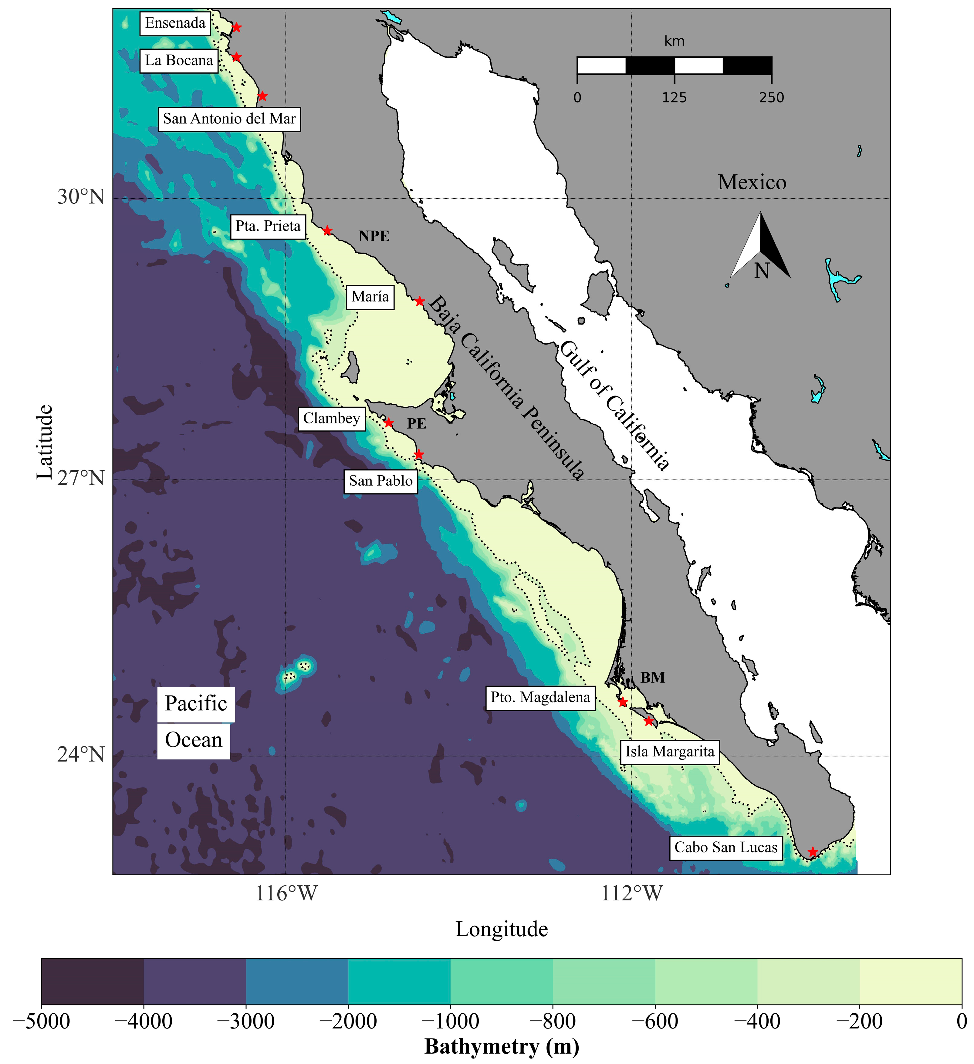
2.1. Study Area
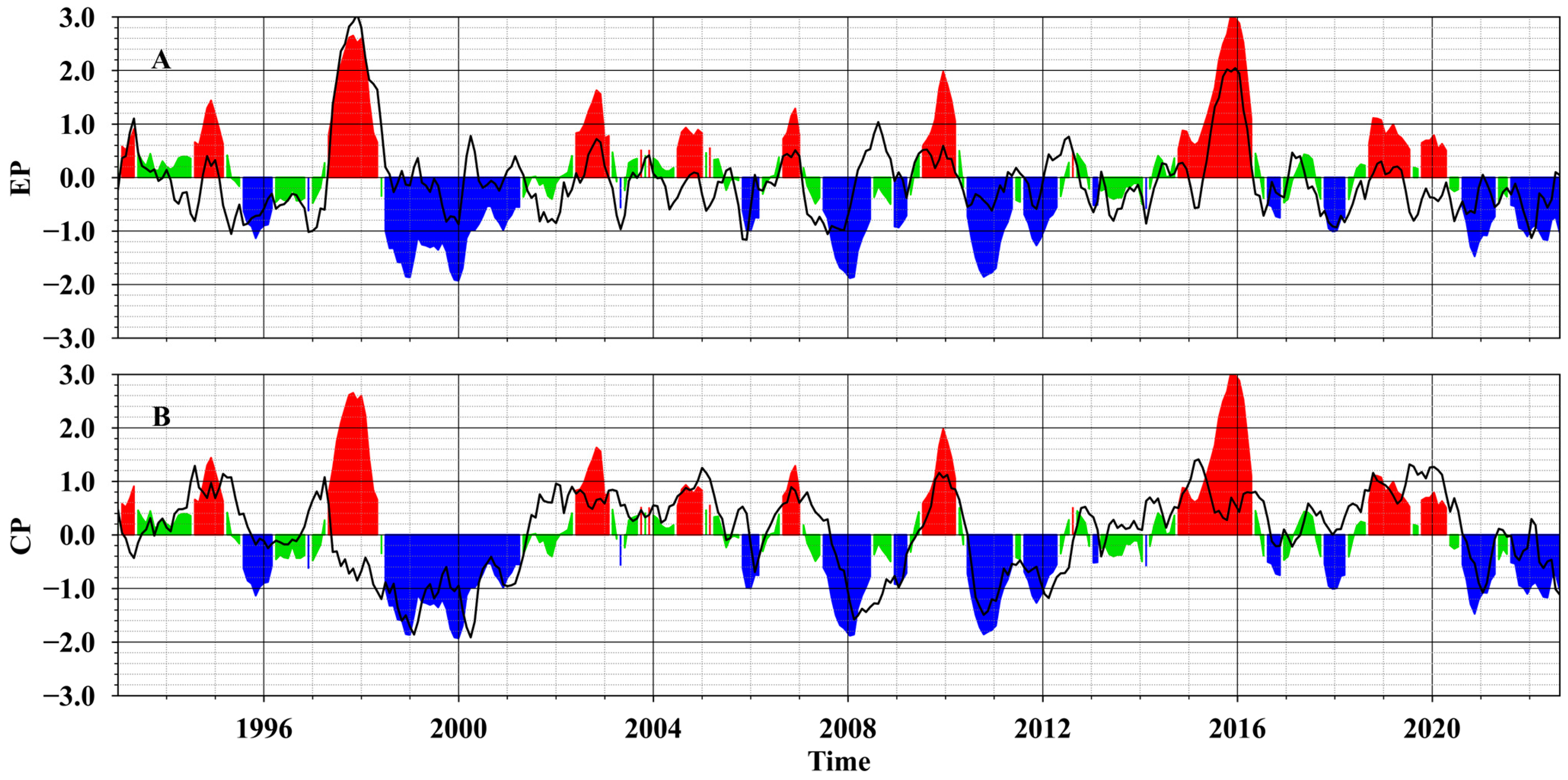
2.2. ENSO Diversity
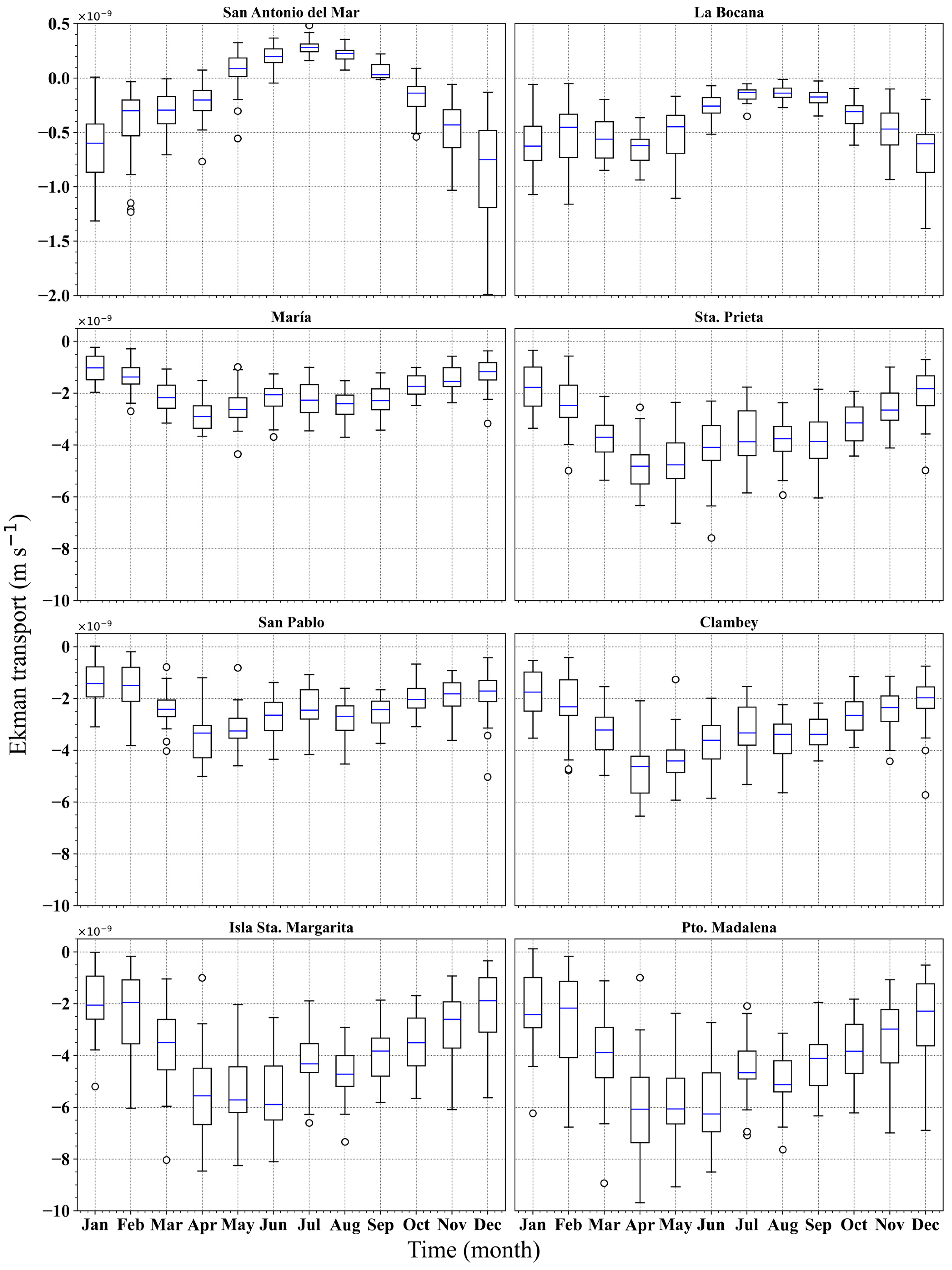
2.3. Wind Data and Ekman Transport
2.4. Sea Surface Chlorophyll-a Concentration
2.5. Wavelet Transform
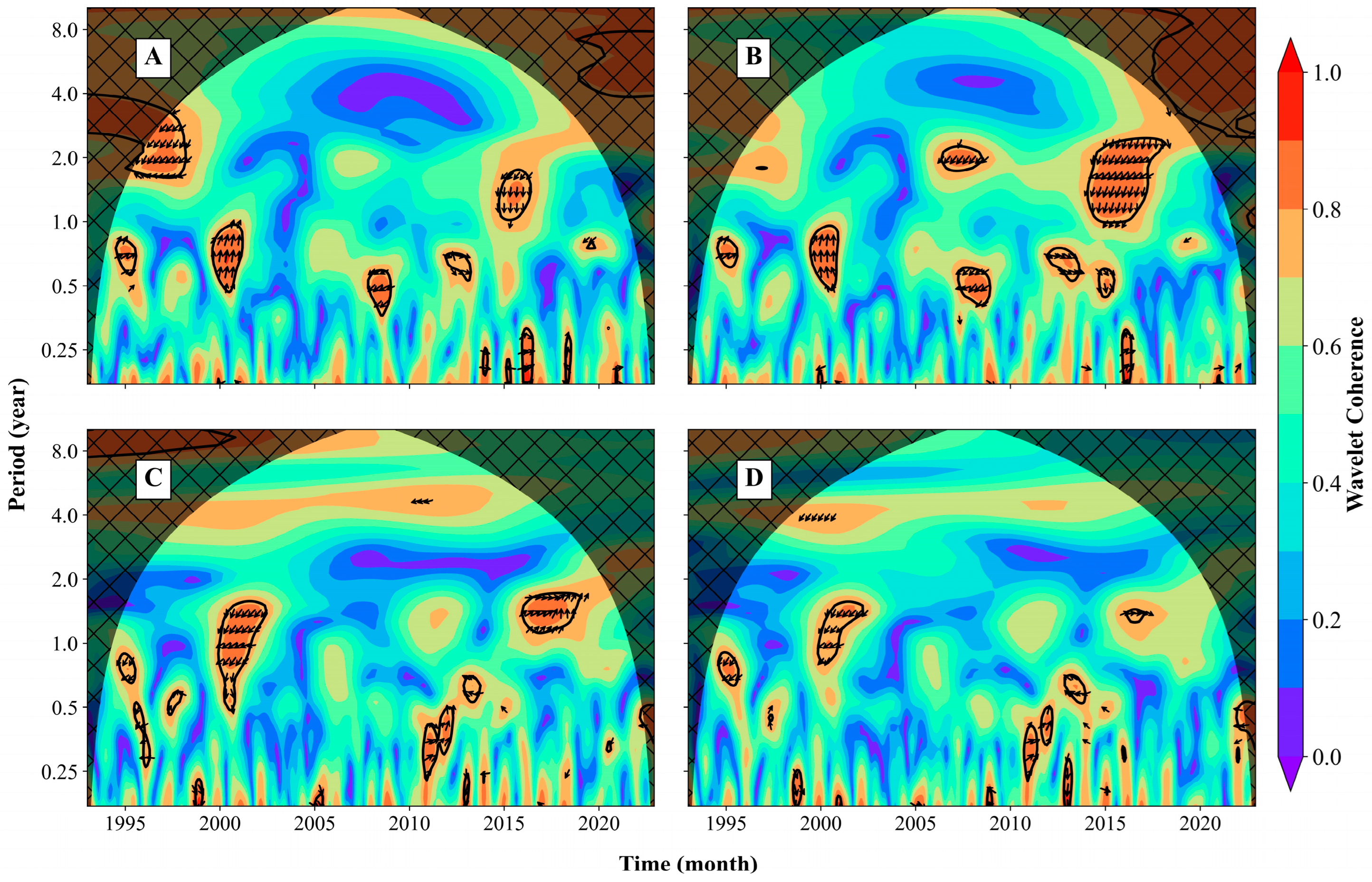
2.6. Wavelet Coherence
3. Results
4. Discussion
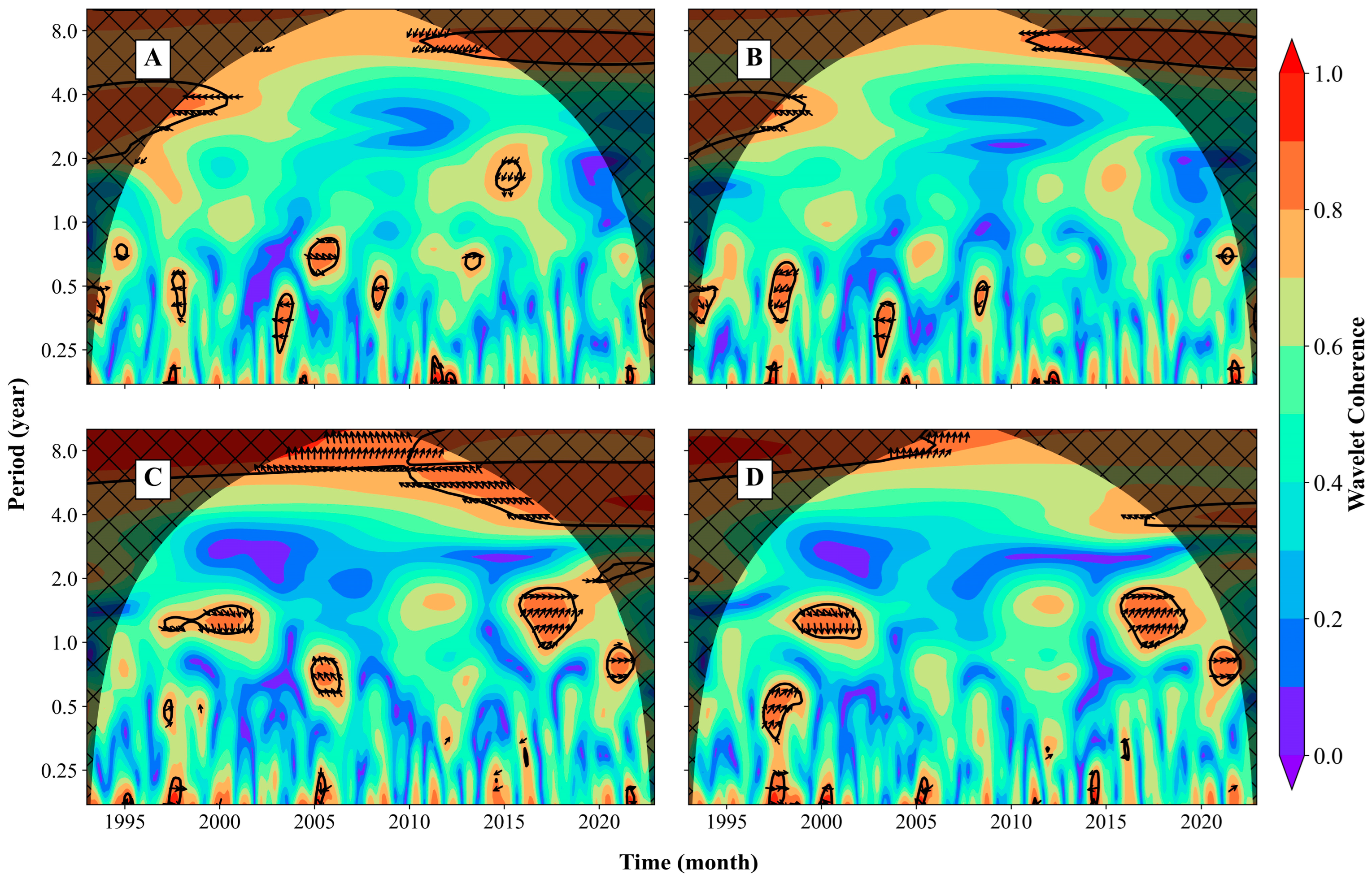
4.1. ENSO and Upwelling Intensity: Interannual Coherence
4.2. Annual and Semiannual Coherence: ENSO and Ekman Transport
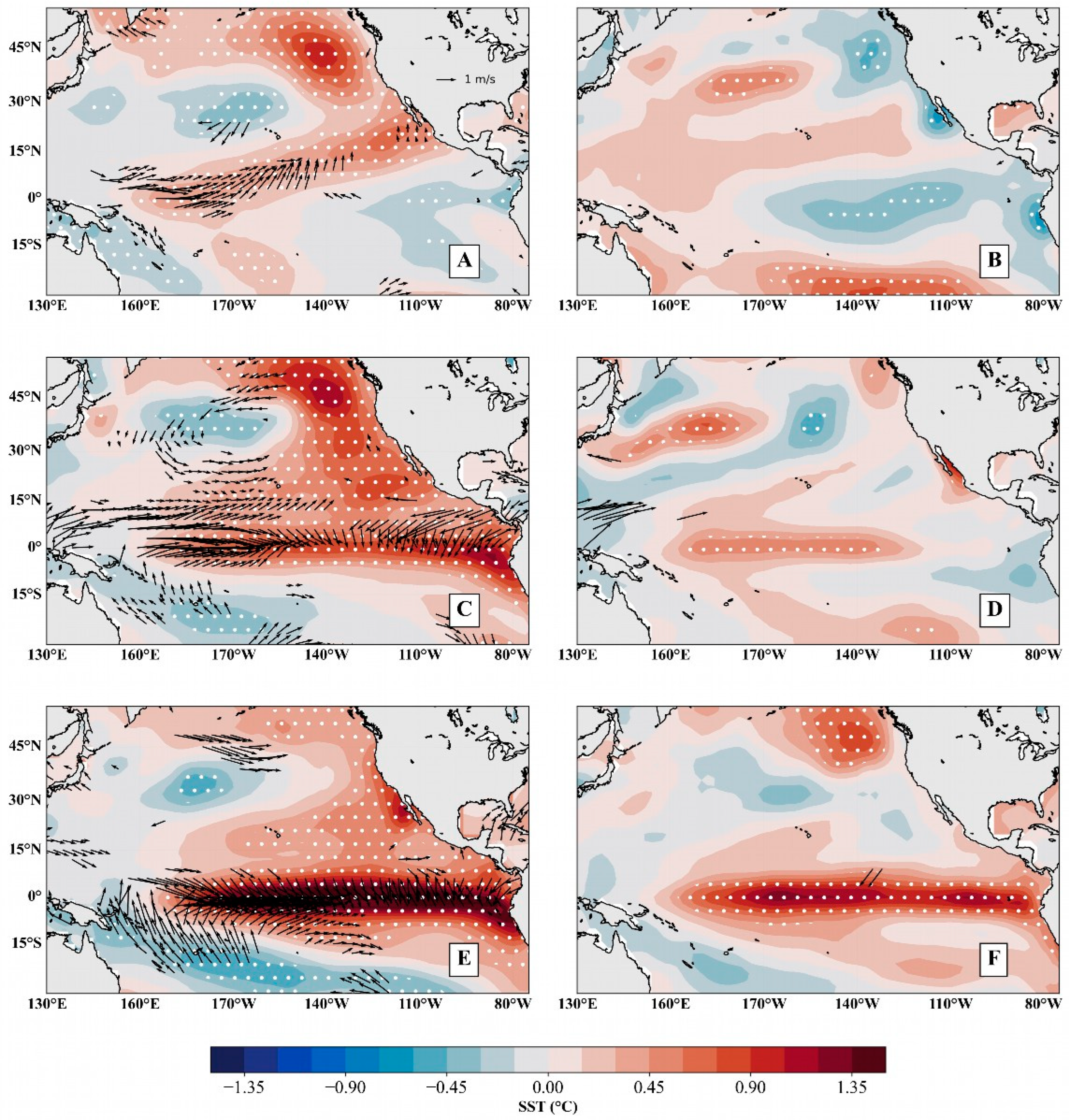
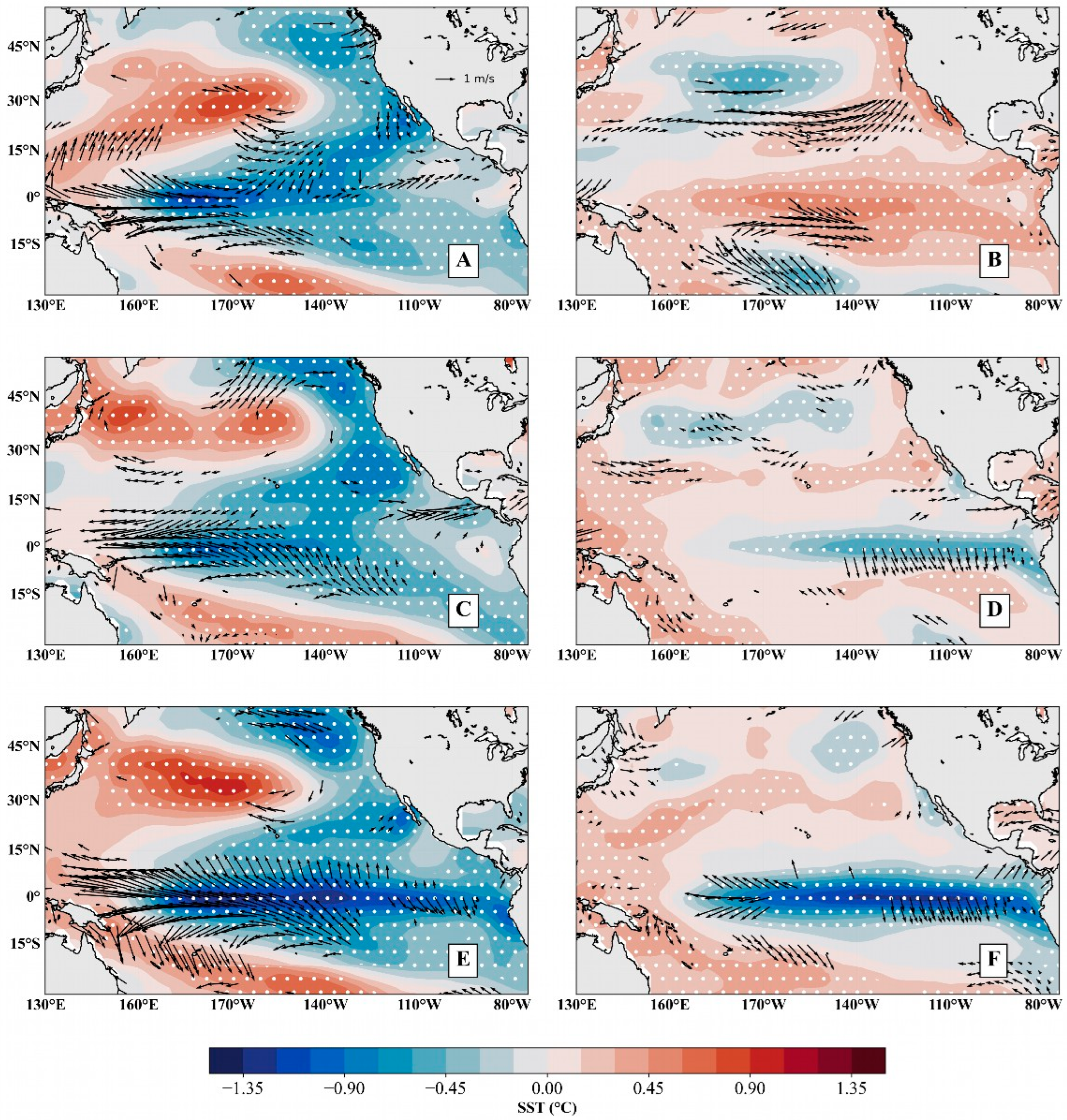
4.3. ENSO Development and Conditions in Pacific for Coherence Events
4.4. ENSO and Biological Response: Interannual Coherence
5. Conclusions
Author Contributions
Funding
Institutional Review Board Statement
Informed Consent Statement
Data Availability Statement
Acknowledgments
Conflicts of Interest
Appendix A


| Event | Phase | Type | Coherence Lead ET (Time Months) | Coherence Chl-a | ||||||
|---|---|---|---|---|---|---|---|---|---|---|
| ENS | NPE | PE | BM | ENS | NPE | PE | BM | |||
| 1994/95 | El Niño | CP | 1–2 * (1–2) | 0 * | 0–4 * | - | - | - | - | |
| 1996/97 | La Niña | EP | - | - | - | - | ||||
| 1997/98 | El Niño | EP | 3–4 | 0–2 | 4–5 | 1–5 | - | - | - | - |
| 1998/99 | La Niña | CP | 1 | |||||||
| 1999/00 | La Niña | CP | c | 2 | 0–2 | 1 | 2 * (2) | 0 * | 0 * | |
| 2001/01 | La Niña | CP | 1–2 * (2–3) | 2 | 0 * | 0 * | ||||
| 2002/03 | El Niño | CP | 0 * | |||||||
| 2004/05 | El Niño | CP | 1 * (2) | |||||||
| 2007/08 | La Niña | CP | 0 | 1–2 * | ||||||
| 2008/09 | La Niña | CP | 0 * | 0 * | 1–2 * | 1 * | 1–4 | |||
| 2009/10 | El Niño | CP | 1–4 | 0–2 | 0–1 * (4–5) | 4 | 1–2 * (2) | 1 (3–4 *) | ||
| I confirm2010/11 | La Niña | CP | 0 | 1–2 * | 21 * | 1–2 | ||||
| 2011/12 | La Niña | CP | 0 | 1–2 * | 0–2 * (4) | 1 * | 2–3 | |||
| 2014/15 | El Niño | CP | 0 * | 4 * | 4–5 | 1–2 * | 0 * (2–3) | |||
| 2015/16 | El Niño | EP | 1–2 * | 4 * | 0–4 | 1–2 * | ||||
| 2017/18 | La Niña | EP | 4–5 | 1–2 | ||||||
| 2018/19 | El Niño | CP | 0 * (0–1) | |||||||
| 2019/20 | El Niño | CP | 1 * | 5 | 0–1 | |||||
| 2020/21 | La Niña | EP | 0 * | |||||||
| 2021/22 | La Niña | CP | 0 | 0 * | ||||||

References
- Bonino, G.; Di Lorenzo, E.; Masina, S.; Iovino, D. Interannual to decadal variability within and across the major Eastern Boundary Upwelling Systems. Sci. Rep. 2019, 9, 19949. [Google Scholar] [CrossRef] [PubMed]
- Pauly, D.; Christensen, V. Primary production sustain global fisheries. Nature 1995, 347, 255–257. [Google Scholar] [CrossRef]
- Messié, M.; Chavez, F.P. Seasonal regulation of primary production in eastern boundary upwelling systems. Prog. Oceanogr. 2015, 134, 1–18. [Google Scholar] [CrossRef]
- Chavez, F.P.; Messié, M. A comparison of Eastern Boundary Upwelling Ecosystems. Prog. Oceanogr. 2009, 83, 80–96. [Google Scholar] [CrossRef]
- Wu, W.; Zhai, F.; Gu, Y.; Liu, C.; Li, P. Weak local upwelling may elevate the risks of harmful algal blooms and hypoxia in shallow waters during the warm season. Environ. Res. Lett. 2023, 18, 114031. [Google Scholar] [CrossRef]
- Villegas, N.; Málikov, I.; Díaz, D. Variabilidad mensual de la velocidad de surgencia y clorofila a en la región del Panama Bight. Rev. Mutis 2016, 6, 82–94. [Google Scholar] [CrossRef]
- Capet, X.; Estrade, P.; Machu, E.; Ndoye, S.; Grelet, J.; Lazar, A.; Marié, L.; Dausse, D.; Brehmer, P. On the dynamics of the southern Senegal upwelling center: Observed variability from synoptic to superinertial scales. J. Phys. Oceanogr. 2017, 47, 155–180. [Google Scholar] [CrossRef]
- Kämpf, J.; Doubell, M.; Griffin, D.; Matthews, R.L.; Ward, T.M. Evidence of a large seasonal coastal upwelling system along the southern shelf of Australia. Geophys. Res. Lett. 2004, 31, 4–7. [Google Scholar] [CrossRef]
- Dang, X.; Bai, Y.; Gong, F.; Chen, X.; Zhu, Q.; Huang, H.; He, X. Different responses of phytoplankton to the ENSO in two upwelling systems of the South China Sea. Estuaries Coasts 2022, 45, 485–500. [Google Scholar] [CrossRef]
- Xiao, F.; Wu, Z.; Lyu, Y.; Zhang, Y. Abnormal strong upwelling off the coast of southeast Vietnam in the late summer of 2016: A comparison with the case in 1998. Atmosphere 2020, 11, 940. [Google Scholar] [CrossRef]
- Rueda-Roa, D.T.; Ezer, T.; Muller-Karger, F.E. Description and mechanisms of the mid-year upwelling in the southern Caribbean Sea from remote sensing and local data. J. Mar. Sci. Eng. 2018, 6, 36. [Google Scholar] [CrossRef]
- Rueda-Roa, D.T.; Muller-Karger, F.E. The southern Caribbean upwelling system: Sea surface temperature, wind forcing and chlorophyll concentration patterns. Deep. Res. Part I Oceanogr. Res. Pap. 2013, 78, 102–114. [Google Scholar] [CrossRef]
- Durazo, R. Climate and upper ocean variability off Baja California, Mexico: 1997–2008. Prog. Oceanogr. 2009, 83, 361–368. [Google Scholar] [CrossRef]
- Durazo, R. Seasonality of the transitional region of the California Current System off Baja California. J. Geophys. Res. Ocean. 2015, 120, 1173–1196. [Google Scholar] [CrossRef]
- González-Silveira, A.; Santamaría-del-Ángel, E.; Camacho-Ibar, V.; López-Calderón, J.; Santander-Cruz, J.; Mercado-Santana, A. The effect of cold and warm anomalies on the phytoplankton pigment composition in waters off northern Baja California Peninsula (México). J. Mar. Sci. Eng. 2020, 8, 533. [Google Scholar] [CrossRef]
- Kahru, M.; Di Lorenzo, E.; Manzano-Sarabia, M.; Mitchell, B.G. Spatial and temporal statistics of sea surface temperature and chlorophyll fronts in the California Current. J. Plankton Res. 2012, 34, 749–760. [Google Scholar] [CrossRef]
- Legaard, K.R.; Thomas, A.C. Spatial patterns in seasonal and interannual variability of chlorophyll and sea surface temperature in the California Current. J. Geophys. Res. Ocean. 2006, 111, 1–21. [Google Scholar] [CrossRef]
- Herrera-Cervantes, H.; Lluch-Cota, S.E.; Lluch-Cota, D.B.; Gutiérrez-de-Velasco, G. Interannual correlations between sea surface temperature and concentration of chlorophyll pigment off Punta Eugenia, Baja California, during different remote forcing conditions. Ocean Sci. 2014, 10, 345–355. [Google Scholar] [CrossRef]
- Todd, R.E.; Rudnick, D.L.; Davis, R.E.; Ohman, M.D. Underwater gliders reveal rapid arrival of El Niño effects off California’s coast. Geophys. Res. Lett. 2011, 38, 1–5. [Google Scholar] [CrossRef]
- Zaytsev, O.; Cervantes-Duarte, R.; Montante, O.; Gallegos-Garcia, A. Coastal upwelling activity on the Pacific shelf of the Baja California Peninsula. J. Oceanogr. 2003, 59, 489–502. [Google Scholar] [CrossRef]
- De la Cruz-Orozco, M.E.; Gómez-Ocampo, E.; Miranda-Bojórquez, L.E.; Cepeda-Morales, J.; Durazo, R.; Lavaniegos, B.E.; Espinosa-Carreón, T.L.; Sosa-Ávalos, R.; Aguirre-Hernández, E.; Gaxiola-Castro, G. Biomasa y producción del fitoplancton frente a la Península de Baja California: 1997–2016. Cienc. Mar. 2017, 43, 217–228. [Google Scholar] [CrossRef]
- Espinosa-Carreon, T.L.; Strub, P.T.; Beier, E.; Ocampo-Torres, F.; Gaxiola-Castro, G. Seasonal and interannual variability of satellite-derived chlorophyll pigment, surface height, and temperature off Baja California. J. Geophys. Res. Ocean. 2004, 109, 1–20. [Google Scholar] [CrossRef]
- Kahru, M.; Mitchell, B.G. Influence of the 1997-98 El Niño on the surface chlorophyll in the California Current. Geophys. Res. Lett. 2000, 27, 2937–2940. [Google Scholar] [CrossRef]
- Kahru, M.; Mitchell, B.G. Influence of the El Niño-La Niña cycle on satellite-derived primary production in the California Current. Geophys. Res. Lett. 2002, 29, 2–5. [Google Scholar] [CrossRef]
- Sosa-Ávalos, R.; Durazo, R.; Mitchell, B.G.; Cepeda-Morales, J.; Gaxiola-Castro, G. Parámetros fotosintéticos frente a Baja California: Una herramienta para estimar la producción primaria con datos de sensores remotos. Cienc. Mar. 2017, 43, 157–172. [Google Scholar] [CrossRef]
- Bograd, S.J.; Lynn, R.J. Physical-biological coupling in the California Current during the 1997-99 El Niño-La Niña cycle. Geophys. Res. Lett. 2001, 28, 275–278. [Google Scholar] [CrossRef]
- Capotondi, A.; Sardeshmukh, P.D.; Di Lorenzo, E.; Subramanian, A.C.; Miller, A.J. Predictability of US west coast ocean temperatures is not solely due to ENSO. Sci. Rep. 2019, 9, 10993. [Google Scholar] [CrossRef] [PubMed]
- Checkley, D.M.; Barth, J.A. Patterns and processes in the California Current System. Prog. Oceanogr. 2009, 83, 49–64. [Google Scholar] [CrossRef]
- Sung, M.K.; Kim, B.M.; An, S.I. Altered atmospheric responses to eastern Pacific and central Pacific El Niños over the North Atlantic region due to stratospheric interference. Clim. Dyn. 2014, 42, 159–170. [Google Scholar] [CrossRef]
- Patricola, C.M.; O’Brien, J.P.; Risser, M.D.; Rhoades, A.M.; O’Brien, T.A.; Ullrich, P.A.; Stone, D.A.; Collins, W.D. Maximizing ENSO as a source of western US hydroclimate predictability. Clim. Dyn. 2020, 54, 351–372. [Google Scholar] [CrossRef]
- Jacox, M.G.; Fiechter, J.; Moore, A.M.; Edwards, C.A. ENSO and the California Current coastal upwelling response. J. Geophys. Res. Ocean. 2015, 120, 1691–1702. [Google Scholar] [CrossRef]
- Ashok, K.; Yamagata, T. The El Niño with a difference. Nature 2009, 461, 481–484. [Google Scholar] [CrossRef] [PubMed]
- Capotondi, A.; Wittenberg, A.T.; Newman, M.; Di Lorenzo, E.; Yu, J.Y.; Braconnot, P.; Cole, J.; Dewitte, B.; Giese, B.; Guilyardi, E.; et al. Understanding ENSO diversity. Bull. Am. Meteorol. Soc. 2015, 96, 921–938. [Google Scholar] [CrossRef]
- Kao, H.Y.; Yu, J.Y. Contrasting Eastern-Pacific and Central-Pacific types of ENSO. J. Clim. 2009, 22, 615–632. [Google Scholar] [CrossRef]
- Takahashi, K.; Montecinos, A.; Goubanova, K.; Dewitte, B. ENSO regimes: Reinterpreting the canonical and Modoki El Niño. Geophys. Res. Lett. 2011, 38, 1–5. [Google Scholar] [CrossRef]
- Di Lorenzo, E.; Xu, T.; Zhao, Y.; Newman, M.; Capotondi, A.; Stevenson, S.; Amaya, D.J.; Anderson, B.T.; Ding, R.; Furtado, J.C.; et al. Modes and mechanisms of Pacific decadal-scale variability. Ann. Rev. Mar. Sci. 2023, 15, 249–275. [Google Scholar] [CrossRef] [PubMed]
- Okumura, Y.M. ENSO diversity from an atmospheric perspective. Curr. Clim. Change Rep. 2019, 5, 245–257. [Google Scholar] [CrossRef]
- Zhang, W.; Wang, Z.; Stuecker, M.F.; Turner, A.G.; Jin, F.F.; Geng, X. Impact of ENSO longitudinal position on teleconnections to the NAO. Clim. Dyn. 2018, 52, 257–274. [Google Scholar] [CrossRef]
- Gutiérrez-Cárdenas, G.S.; Díaz, D.C. El Niño-Southern Oscillation diversity and its relationship with the North Atlantic Oscillation—Atmospheric anomalies response over the North Atlantic and the Pacific. Atmosfera 2024, 38, 129–149. [Google Scholar] [CrossRef]
- Kim, H.-M.; Webster, P.J.; Curry, J.A. Ocean warming on North Atlantic tropical cyclones. Science 2009, 77, 77–80. [Google Scholar] [CrossRef]
- Beltrán, L.; Díaz, D.C. Oscilaciones macroclimáticas que afectan la oferta hídrica en la Cuenca del Río Gachaneca; Boyacá-Colombia. Rev. Bras. Meteorol. 2020, 35, 171–185. [Google Scholar] [CrossRef]
- Navarro-Monterroza, E.; Arias, P.A.; Vieira, S.C. El Niño/Southern Oscillation Modoki and its effects on the spatiotemporal variability of precipitation in Colombia. Rev. Acad. Colomb. Cienc. Exactas Fís. Nat. 2019, 43, 120–132. [Google Scholar] [CrossRef]
- Salas, H.D.; Poveda, G.; Mesa, Ó.J.; Marwan, N. Generalized synchronization between ENSO and hydrological variables in Colombia: A recurrence quantification approach. Front. Appl. Math. Stat. 2020, 6, 3. [Google Scholar] [CrossRef]
- Tedeschi, R.G.; Cavalcanti, I.F.A.; Grimm, A.M. Influences of two types of ENSO on South American precipitation. Int. J. Climatol. 2013, 33(6), 1382–1400. [Google Scholar] [CrossRef]
- Cai, W.; McPhaden, M.J.; Grimm, A.; Rodrigues, R.; Taschetto, A.; Garreaud, R.; Dewitte, B.; Germán, P.; Ham, Y.-G.; Santoso, A.; et al. Climate impacts of the El Niño—Southern Oscillation on South America. Nat. Rev. Earth Environ. 2020, 1, 215–231. [Google Scholar] [CrossRef]
- Li, Y.; Lau, N.C. Impact of ENSO on the atmospheric variability over the North Atlantic in late winter-role of transient eddies. J. Clim. 2012, 25, 320–342. [Google Scholar] [CrossRef]
- Zhang, W.; Wang, L.; Xiang, B.; Qi, L.; He, J. Impacts of two types of La Niña on the NAO during boreal winter. Clim. Dyn. 2015, 44, 1351–1366. [Google Scholar] [CrossRef]
- Chen, M.; Yu, J.-Y.; Wang, X.; Jiang, W. The Changing impact mechanisms of a diverse El Niño on the western Pacific Subtropical high. Geophys. Res. Lett. 2019, 46, 956–962. [Google Scholar] [CrossRef]
- Racault, M.F.; Sathyendranath, S.; Brewin, R.J.W.; Raitsos, D.E.; Jackson, T.; Platt, T. Impact of El Niño variability on oceanic phytoplankton. Front. Mar. Sci. 2017, 4, 133. [Google Scholar] [CrossRef]
- Lehodey, P.; Bertrand, A.; Hobday, A.J.; Kiyofuji, H.; McClatchie, S.; Menkès, C.E.; Pilling, G.; Polovina, J.; Tommasi, D. ENSO Impact on Marine Fisheries and Ecosystems. Chapter 19. In El Niño Southern Oscillation in a Changing Climate; McPhaden, M.J., Santoso, A., Cai, W., Eds.; AGU Publications: Washington, DC, USA, 2020; pp. 429–451. [Google Scholar] [CrossRef]
- Yu, J.-Y.; Kao, H.-Y.; Lee, T. Subtropics-related interannual sea surface temperature variability in the central Equatorial Pacific. Am. Meteorol. Soc. 2010, 23, 2869–2884. [Google Scholar] [CrossRef]
- Wang, X.; Guan, C.; Xin, R.; Wei, H.; Wang, L. The roles of tropical and subtropical wind stress anomalies in the El Niño Modoki onset. Clim. Dyn. 2019, 52, 6585–6597. [Google Scholar] [CrossRef]
- Amaya, D.J. The Pacific Meridional Mode and ENSO: A Review. Curr. Clim. Change Rep. 2019, 5, 296–307. [Google Scholar] [CrossRef]
- Kug, J.S.; Jin, F.F.; An, S. Il Two types of El Niño events: Cold tongue El Niño and warm pool El Niño. J. Clim. 2009, 22, 1499–1515. [Google Scholar] [CrossRef]
- Yeh, S.W.; Kug, J.S.; Dewitte, B.; Kwon, M.H.; Kirtman, B.P.; Jin, F.F. El Niño in a changing climate. Nature 2009, 461, 511–514. [Google Scholar] [CrossRef]
- Lee, T.; McPhaden, M.J. Increasing intensity of El Niño in the central-equatorial Pacific. Geophys. Res. Lett. 2010, 37, 1–5. [Google Scholar] [CrossRef]
- López-Aviles, B.; Beier, E.; Duran, R.; Gómez-Valdés, J.; Castro, R.; Sánchez-Velasco, L. The California Current System off Baja California Sur. Prog. Oceanogr. 2024, 222, 103225. [Google Scholar] [CrossRef]
- Kurczyn, J.A.; Beier, E.; Lavín, M.F.; Chaigneau, A. Mesoscale eddies in the northeastern Pacific tropical-subtropical transition zone: Statistical characterization from satellite altimetry. J. Geophys. Res. Ocean. 2012, 117, 1–17. [Google Scholar] [CrossRef]
- Espinosa-Carreón, T.L.; Gaxiola-Castro, G.; Beier, E.; Strub, P.T.; Kurczyn, J.A. Effects of mesoscale processes on phytoplankton chlorophyll off Baja California. J. Geophys. Res. Ocean. 2012, 117, C04005. [Google Scholar] [CrossRef]
- Castro, R.; Martínez, J.A. Variabilidad espacial y temporal del campo de viento. Dinámica del ecosistema pelágico frente a Baja California. In Dinámica del Ecosistema Pelágico Frente a Baja California 1997–2007, Diez años de investigaciones mexicanas de la Corriente de California; Gaxiola-Castro, G., Durazo, R., Eds.; Centro de Investigaciones Científicas y de Educación Superior de Ensenada: UABC; SEMARNAT: Instituto Nacional de Ecología: Ensenada, Mexico, 2010; pp. 129–147. ISBN 978-607-7908-30-2. [Google Scholar]
- Vazquez, H.J.; Gomez-Valdes, J. Wind events in a subtropical coastal upwelling region as detected by admittance analysis. Ocean Dyn. 2021, 71, 631. [Google Scholar] [CrossRef]
- Sullivan, A.; Luo, J.J.; Hirst, A.C.; Bi, D.; Cai, W.; He, J. Robust contribution of decadal anomalies to the frequency of central-Pacific El Niño. Sci. Rep. 2016, 6, 38540. [Google Scholar] [CrossRef]
- Santamaría-del-Ángel, E.; Sebastia-Frasquet, M.T.; González-Silveira, A.; Aguilar-Maldonado, J.; Mercado-Santana, A.; Herrera-Carmona, J.C. Uso potencial de las anomalías estandarizadas en la interpretación de fenómenos oceanográficos globales a escalas locales. In Tópicos de Agenda para la Sostenibilidad de Costas y Mares Mexicanos; Rivera-Arriaga, E., Sánchez-Gil, P., Gutiérrez, J., Eds.; Red RICOMAR; Universidad Autónoma de Campeche: Campeche, Mexico, 2019; pp. 193–211. ISBN 978-607-844-57-1. [Google Scholar]
- Atlas, R.; Hoffman, R.N.; Ardizzone, J.; Leidner, S.M.; Jusem, J.C.; Smith, D.K.; Gombos, D. A cross-calibrated, multiplatform ocean surface wind velocity product for meteorological and oceanographic applications. Bull. Am. Meteorol. Soc. 2011, 92, 157–174. [Google Scholar] [CrossRef]
- Ray, S.; Swain, D. A systematic method of estimation of alongshore windstress and Ekman transport associated with coastal upwelling. MethodsX 2023, 10, 102186. [Google Scholar] [CrossRef] [PubMed]
- Thomson, R.E.; Emery, W.J. Data Analysis in Physical Oceanography, 3rd ed.; Elsevier: Oxford, UK, 2014; ISBN 9780123877826. [Google Scholar]
- Díaz, D.; Villegas, N. Wavelet coherence between ENSO indices and two precipitation databases for the Andes region of Colombia. Atmosfera 2022, 35, 237–271. [Google Scholar] [CrossRef]
- Das, J.; Jha, S.; Goyal, M.K. On the relationship of climatic and monsoon teleconnections with monthly precipitation over meteorologically homogenous regions in India: Wavelet & global coherence approaches. Atmos. Res. 2020, 238, 104889. [Google Scholar] [CrossRef]
- Veleda, D.; Montagne, R.; Araujo, M. Cross-wavelet bias corrected by normalizing scales. Am. Meteorol. Soc. 2012, 29, 1401–1408. [Google Scholar] [CrossRef]
- Grinsted, A.; Moore, J.C.; Jevrejeva, S. Application of the cross wavelet transform and wavelet coherence to geophysical time series. Nonlinear analysis of multivariate geoscientific data—Advanced methods, theory and application. Nonlinear Process. Geophys. 2004, 11, 561–566. [Google Scholar] [CrossRef]
- Torrence, C.; Compo, G.P. A Practical Guide to Wavelet Analysis. Bull. Am. Meteorol. Soc. 1998, 79(1), 61–78. [Google Scholar] [CrossRef]
- Barnard, P.L.; Hoover, D.; Hubbard, D.M.; Snyder, A.; Ludka, B.C.; Allan, J.; Kaminsky, G.M.; Ruggiero, P.; Gallien, T.W.; Gabel, L.; et al. Extreme oceanographic forcing and coastal response due to the 2015–2016 El Niño. Nat. Commun. 2017, 8, 6–13. [Google Scholar] [CrossRef]
- Cai, W.; Santoso, A.; Collins, M.; Dewitte, B.; Karamperidou, C.; Kug, J.-S.; Lengaigne, M.; McPhaden, M.J.; Stuecker, M.F.; Taschetto, A.S.; et al. Changing El Niño–Southern Oscillation in a warming climate. Nat. Rev. Earth Environ. 2021, 2, 628–644. [Google Scholar] [CrossRef]
- Linacre, L.; Durazo, R.; Hernández-Ayón, J.M.; Delgadillo-Hinojosa, F.; Cervantes-Díaz, G.; Lara-Lara, J.R.; Camacho-Ibar, V.; Siqueiros-Valencia, A.; Bazán-Guzmán, C. Temporal variability of the physical and chemical water characteristics at a coastal monitoring observatory: Station ENSENADA. Cont. Shelf Res. 2010, 30, 1730–1742. [Google Scholar] [CrossRef]
- McPhaden, M.J. Evolution of the 2002/03 El Niño. Am. Meteorol. Soc. 2004, 85(5), 677–695. [Google Scholar] [CrossRef]
- Chen, S.; Chen, W.; Yu, B.; Wu, R.; Graf, H.F.; Chen, L. Enhanced impact of the Aleutian Low on increasing the Central Pacific ENSO in recent decades. npj Clim. Atmos. Sci. 2023, 6, 29. [Google Scholar] [CrossRef]
- Anderson, B.T.; Perez, R.C.; Karspeck, A. Triggering of El Niño onset through trade wind—Induced charging of the equatorial Pacific. Geophys. Res. Lett. 2013, 40, 1212–1216. [Google Scholar] [CrossRef]
- Schwing, F.B.; Murphree, T.; Green, P.M. The evolution of oceanic and atmospheric anomalies in the northeast Pacific during El Niño and La Niña events of 1995-2001. Prog. Oceanogr. 2002, 54, 459–491. [Google Scholar] [CrossRef]
- Xie, S.P. A Dynamic ocean—atmosphere model of the Tropical Atlantic decadal variability. J. Clim. 1999, 12, 64–70. [Google Scholar] [CrossRef]
- Hartman, D. Pacific sea surface temperature and winter of 2014. Geophys. Res. Lett. 2015, 42, 1894–1902. [Google Scholar] [CrossRef]
- Chen, S.; Chen, W.; Wu, R.; Yu, B.; Graf, H.F. Potential impact of preceding Aleutian low variation on El Niño–Southern oscillation during the following winter. J. Clim. 2020, 33, 3061–3077. [Google Scholar] [CrossRef]
- Amaya, D.J.; Miller, A.J.; Xie, S. Kosaka Physical drivers of the summer 2019 North Pacific marine heathwave. Nat. Commun. 2019, 11, 1903. [Google Scholar] [CrossRef] [PubMed]
- Di Lorenzo, E.; Combes, V.; Keister, J.E.; Strub, P.T.; Thomas, A.C.; Franks, P.J.S.; Ohman, M.D.; Furtado, J.C.; Bracco, A.; Bograd, S.J.; et al. Synthesis of Pacific Ocean climate and ecosystem dynamics. Oceanography 2013, 26, 68–81. [Google Scholar] [CrossRef]
- Ashok, K.; Behera, S.K.; Rao, S.A.; Weng, H.; Yamagata, T. El Niño Modoki and its possible teleconnection. J. Geophys. Res. Ocean. 2007, 112, 1–27. [Google Scholar] [CrossRef]
- Zhao, J.; Kug, J.; Park, J.-H.; An, S.I. Diversity of North Pacific meridional mode and its distinct impacts on El Niño-Southern Oscillation. Geophys. Res. Lett. 2020, 47, e2020GL088993. [Google Scholar] [CrossRef]
- Yang, S.; Li, Z.; Yu, J.Y.; Hu, X.; Dong, W.; He, S. El Niño-Southern Oscillation and its impact in the changing climate. Natl. Sci. Rev. 2018, 5, 840–857. [Google Scholar] [CrossRef]
- Rogers, J.C. The North Pacific oscillation. J. Climatol. 1981, 1, 39–57. [Google Scholar] [CrossRef]
- Vimont, D.J.; Wallace, J.M.; Battisti, D.S. The seasonal footprinting mechanism in the Pacific: Implications for ENSO. J. Clim. 2003, 16, 2668–2675. [Google Scholar] [CrossRef]
- Vimont, D.J.; Battisti, D.S.; Hirts, A.C. Footprinting: A seasonal connection between the tropics and mid-latitudes. Geophys. Res. Lett. 2001, 28, 3923–3926. [Google Scholar] [CrossRef]


| El Niño | La Niña | |
|---|---|---|
| EP | 1997/98, 2015/16 | 1996/97, 2017/18, 2021/22 |
| CP | 1994/95, 2002/03, 2004/05, 2009/10, 2014/15, 2018/19, 2019/20 | 1998/99, 1999/00, 2000/01, 2007/08, 2008/09, 2010/11, 2011/12, 2020/21 |
| Region | Upwelling Center | Long Term Mean (m s−1) | Standard Deviation | Month (Minimum Value) |
|---|---|---|---|---|
| Bahía Magdalena | Isla Santa Margarita | −3.82 × 10⁻⁹ | 1.82 × 10⁻⁹ | June (−5.58 × 10⁻⁹) |
| Puerto Magdalena | −4.18 × 10⁻⁹ | 1.96 × 10⁻⁹ | June (−5.94 × 10⁻⁹) | |
| Punta Eugenia | San Pablo | −2.34 × 10⁻⁹ | 0.97 × 10⁻⁹ | April (−3.43 × 10⁻⁹) |
| Clambey | −3.12 × 10⁻⁹ | 1.24 × 10⁻⁹ | April (−4.71 × 10⁻⁹) | |
| North of Punta Eugenia | María | −1.95 × 10⁻⁹ | 0.79 × 10⁻⁹ | April (−2.85 × 10⁻⁹) |
| Punta Prieta | −3.38 × 10⁻⁹ | 1.35 × 10⁻⁹ | April (−4.85 × 10⁻⁹) | |
| Ensenada | San Antonio del Mar | −1.85 × 10⁻¹⁰ | 4.13 × 10⁻¹⁰ | December (−1.98 × 10⁻⁹) |
| La Bocana | −4.21 × 10⁻¹⁰ | 2.73 × 10⁻¹⁰ | December (−1.37 × 10⁻⁹) |
Disclaimer/Publisher’s Note: The statements, opinions and data contained in all publications are solely those of the individual author(s) and contributor(s) and not of MDPI and/or the editor(s). MDPI and/or the editor(s) disclaim responsibility for any injury to people or property resulting from any ideas, methods, instructions or products referred to in the content. |
© 2024 by the authors. Licensee MDPI, Basel, Switzerland. This article is an open access article distributed under the terms and conditions of the Creative Commons Attribution (CC BY) license (https://creativecommons.org/licenses/by/4.0/).
Share and Cite
Gutiérrez-Cárdenas, G.S.; Morales-Acuña, E.; Tenorio-Fernández, L.; Gómez-Gutiérrez, J.; Cervantes-Duarte, R.; Aguíñiga-García, S. El Niño–Southern Oscillation Diversity: Effect on Upwelling Center Intensity and Its Biological Response. J. Mar. Sci. Eng. 2024, 12, 1061. https://doi.org/10.3390/jmse12071061
Gutiérrez-Cárdenas GS, Morales-Acuña E, Tenorio-Fernández L, Gómez-Gutiérrez J, Cervantes-Duarte R, Aguíñiga-García S. El Niño–Southern Oscillation Diversity: Effect on Upwelling Center Intensity and Its Biological Response. Journal of Marine Science and Engineering. 2024; 12(7):1061. https://doi.org/10.3390/jmse12071061
Chicago/Turabian StyleGutiérrez-Cárdenas, Gabriel Santiago, Enrique Morales-Acuña, Leonardo Tenorio-Fernández, Jaime Gómez-Gutiérrez, Rafael Cervantes-Duarte, and Sergio Aguíñiga-García. 2024. "El Niño–Southern Oscillation Diversity: Effect on Upwelling Center Intensity and Its Biological Response" Journal of Marine Science and Engineering 12, no. 7: 1061. https://doi.org/10.3390/jmse12071061