Article

Task-Driven Learning Downsampling Network Based Phase-Resolved Wave Fields Reconstruction with Remote Optical Observations

College of Marine Electrical Engineering, Dalian Maritime University, Dalian 116026, China
*
Author to whom correspondence should be addressed.
J. Mar. Sci. Eng. 2024, 12(7), 1082; https://doi.org/10.3390/jmse12071082
Submission received: 4 June 2024 / Revised: 22 June 2024 / Accepted: 25 June 2024 / Published: 27 June 2024
(This article belongs to the Section Ocean Engineering)

Abstract

:
We develop a phase-resolved wave field reconstruction method by the learning-based downsampling network for processing large amounts of inhomogeneous data from non-contact wave optical observations. The Waves Acquisition Stereo System (WASS) extracts dense point clouds from ocean wave snapshots. We couple learning-based downsampling networks with the phase-resolved wave reconstruction algorithm, and the training task is to improve the wave reconstruction completeness ratio C R . The algorithm first achieves initial convergence and task-optimized performance on numerical ocean waves built by the linear wave theory model. Results show that the trained sampling network can lead to a more uniform spatial distribution of sampling points and improve C R at the observed edge regions far from the optical camera. Finally, we apply our algorithm to a natural ocean wave dataset. The average completeness ratio is improved over 30% at low sampling ratios ( S R [ 2 9 , 2 7 ] ) compared to the traditional FPS method and Random sampling method. Moreover, the relative residual between the final reconstructed wave and the natural wave is less than 15%, which provides an efficient tool for wave reconstruction in ocean engineering.

1. Introduction

The rapid and real-time reconstruction of ocean wave elevation has critical applications in marine engineering, such as providing decision support for unmanned ships, optimizing marine equipment, and conducting safety analyses of offshore operations [1,2]. Most research on wave surface reconstruction involves fitting the wave surface by interpolating observed discrete wave points, which is limited to specific application scenarios [3,4,5]. In contrast, phase-resolved modeling offers an instantaneous representation of ocean wave motion and statistical properties related to surface wave dynamics [6]. This method is extensively employed for linear deterministic wave prediction and the wave load calculation [7,8,9,10,11]. Constructing a phase-resolved wave field and inverting the wave dynamic models necessitates high spatial resolution of wave observation points [12,13]. Additionally, the wave shadow effect and the uneven distribution of measurement points hinder the development of inversion algorithms and the accuracy of reconstruction [14,15,16]. To address these challenges, we propose a phase-resolved wave field reconstruction method via the learning-based downsampling network. This framework processes substantial amounts of inhomogeneous data from non-contact wave observations, and provides an optimal sampling strategy for downstream wave inversion tasks.
To reconstruct the phase-resolved wave field, observations must encompass a sufficiently large area and possess a high spatial resolution [17]. Traditional methods, such as wave staffs/buoys and X-band radars, face issues regarding the number of measured points and the spatial resolution, respectively [18,19,20,21]. LiDAR is a powerful remote sensing tool, and has been widely used in the marine, offshore and coastal fields [22,23]. Although LiDAR cameras offer higher spatial resolution and can directly measure wave elevation via the time-of-flight method, they are constrained by wavefront conditions, requiring an aerated and turbulent water surface [24,25]. Stereo imaging technology, employing high-resolution cameras, provides high-precision observations of the sea surface, and is relatively inexpensive and widely applicable [26]. Consequently, we utilize this method for data acquisition in this study. However, when stereo imaging technology operates at a grazing angle, it suffers from a spatially inhomogeneous distribution of measurement points. Since the reconstruction relies on the observation points, an uneven distribution of these points can lead to the loss of wave information, thereby negatively affecting the reconstruction accuracy at the edges of the observed region. Additionally, the extensive volume of point cloud data poses significant challenges for the rapid reconstruction of the phase-resolved wave field directly from the acquired points [27,28].
Point cloud sampling methods can reduce the data size while altering the distribution of observation points to enhance the performance and computational efficiency of reconstruction tasks. Traditional sampling methods include Random Sampling (RS), Grid Sampling, Kd-tree Sampling, and Farthest Point Sampling (FPS) [29,30]. The FPS method is widely used because it effectively preserves the overall features of the point cloud, though it is limited in processing large-scale point cloud data [31]. Recently, many deep learning-based point cloud downsampling methods have been proposed. Geometric deep learning-based point cloud compression employs techniques, such as local feature extraction and local feature aggregation, to achieve point cloud compression [32]. K-means clustering was first used to select representative points and to remove redundant points [33]. Furthermore, a combination of clustering and coarse-to-fine methods has been proposed to achieve fast point cloud simplification [34]. PointNetLK-CPD utilizes the PointNetLK and coherent point drift algorithms to perform unsupervised point cloud compression [35]. Neural Point Cloud Compression extracts point cloud feature information by learning optical flow representations, enabling high-ratio point cloud simplification while preserving geometric features [35]. These deep learning-based point cloud downsampling methods predominantly focus on the geometric structure information of the point cloud, achieving outstanding performance in various point cloud processing tasks. However, they cannot dynamically adjust the sampling strategy according to the requirements of different tasks, thereby affecting the performance of downstream tasks.
Task-driven point cloud downsampling methods have emerged in recent years, dynamically learning sampling strategies based on task requirements to enhance the performance of downstream tasks [36,37,38]. S-Net was the first to propose the idea of learning-based sampling, making the sampled points more adaptable to various tasks and application needs [39]. APSNet is an attention-based point cloud sampling network that focuses on all points by exploiting the history of previously sampled points to find the optimal sampling strategy to optimize the performance of various downstream tasks [40]. LighTN introduced a novel single-head self-correlation module and a sampling loss function, achieving state-of-the-art performance in preserving geometric features across various downstream tasks [41]. Skeleton-Guided Learning proposes a sampling method to preserve the object geometry and topology information during sampling [42,43]. REPS introduced the Global-Local Fusion Attention (GLFA) module, effectively integrating local and global features of the point cloud, thereby ensuring the quality of reconstruction tasks and downsampling [44]. The results of these studies indicate that task-driven point cloud downsampling methods can significantly enhance the performance of downstream tasks.
For wave reconstruction in ocean engineering, embedding physics-based numerical methods within data-driven approaches can enhance the performance of wave model acquisition and wave reconstruction tasks. When predicting waves at specific locations, artificial neural networks (ANNs) serve as effective supplementary tools to physical wave models, boosting their efficiency and reliability. By training ANNs to learn the discrepancies between wave model outputs and measured values, the accuracy of wave models can be improved [45]. Additionally, machine learning can reduce subjectivity and improve modeling accuracy by understanding the sources of uncertainty and quantifying parameter selection in coastal ocean modeling [46]. Bias correction techniques can effectively align wave model outputs with observational data, addressing model inaccuracies [47]. Bagged regression trees (BRT) have been used to predict and describe systematic errors in significant wave height model forecasts, helping to identify areas in the model output space that require refinement [48]. The combination of physical models like Simulating Waves Nearshore (SWAN) with machine learning algorithms (such as BRT and ANN) can be employed to estimate wave parameters in shallow estuaries and identify sources of error in physical models [49]. The physics-informed neural network model NWnets integrates prior knowledge of wave mechanics into soft computing deep learning algorithms, enabling efficient reconstruction of nearshore wave fields with limited measurements [50]. However, these studies neglect the effect of downsampling on wave reconstruction tasks.
Overall, existing research primarily focuses on leveraging networks and models to reduce the inherent errors within the models themselves. However, to the best of the authors’ knowledge, errors stemming from data input have not received adequate attention. Building on the concept of integrating data-driven approaches with physical models from prior studies, this paper proposes a learning-based downsampling strategy to identify the optimal input point cloud for downstream reconstruction tasks. Addressing errors from the perspective of data input minimizes the phase-resolved wave field reconstruction errors and ensures a uniform distribution of the downsampled point cloud. This approach opens up new possibilities for developing novel wave inversion algorithms. This manuscript is organized as follows: In Section 2, the proposed algorithm is described in detail. Section 3 reviews the background of phase-resolved wave field reconstruction, specifically focusing on linear wave theory and the numerical methods for solving wave model parameters. Additionally, we detail the construction of the dataset. Section 4 presents and discusses the test results of the proposed methodology. Conclusions are provided in the final section.

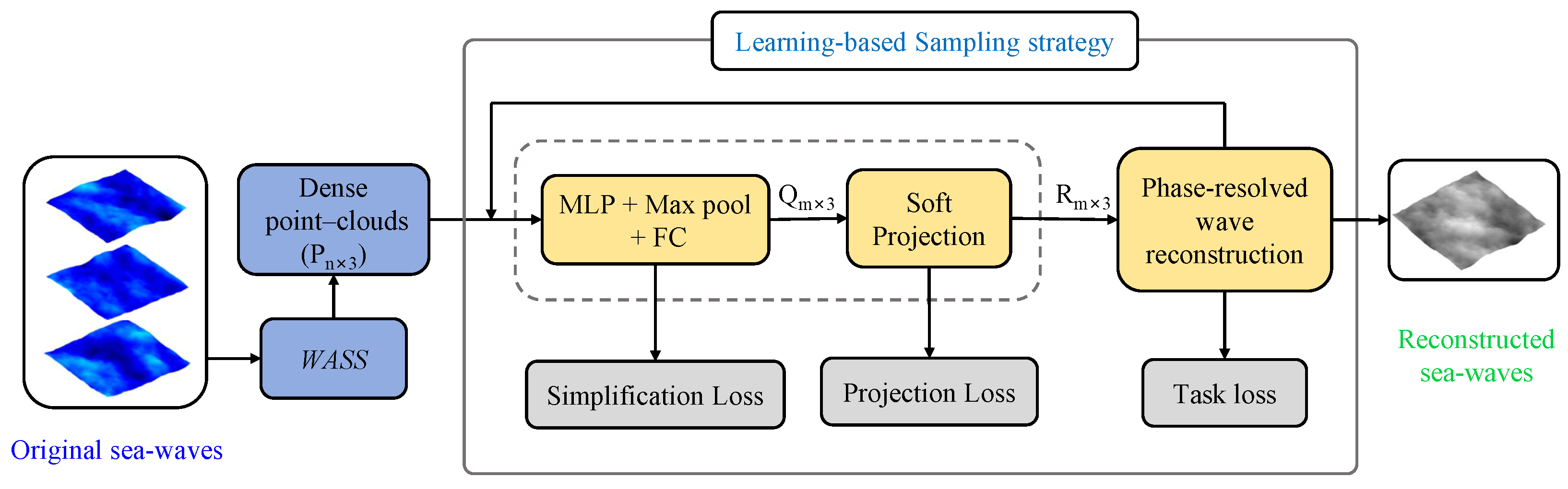
2. Proposed Methodology

To enhance the accuracy of real-time wave field reconstruction based on remote optical measurements, in this study, we developed a learning-based downsampling network. We defined a total loss function that considers task loss and sampling loss as the optimization objective to obtain the optimal input point cloud for downstream reconstruction tasks. The downsampling network comprises a point cloud simplification network and a soft projection operation, enabling sampling at any predetermined ratio. The resulting point cloud satisfies task optimality, similarity to the original point cloud, and distribution uniformity at the specified sampling ratio. The overall optimization framework for the task is illustrated in Figure 1. The dense wave point cloud P n × 3 is obtained by initializing the input wave stereo image pairs through the WASS pipeline [51], which contains 3D position information of n wave observation points, and is used as input data for the network. The data volume of P n × 3 is compressed to m by the simplified network to form a point cloud Q m × 3 with a smaller data volume, and the sampled output point cloud R m × 3 is obtained by soft-projecting Q m × 3 onto P m × 3 . This step is used to further ensure the proximity between the simplified point cloud Q and the original point cloud P. This output serves as an input to the wave reconstruction algorithm for the downstream task. The sampling network is trained to obtain the optimal sampling strategy by minimizing the task loss based on the phase-resolved wave reconstruction. After converging, reconstructed sea-waves are exported. Next, we introduce the construction of learning-based sampling network and the algorithm of phase-resolved wave reconstruction.
Our objective is to extract an optimal point cloud subset R * R m × 3 from the original point cloud P R n × 3 to enhance the performance of the downstream wave reconstruction task T. We define the optimization problem as follows:
R * = argmin R F ( T ( R ) ) , with R P , m n ,
where R R m × 3 represents the variation in the point cloud during training. To address this optimization problem, we employ a simplified network model based on multilayer perceptrons (MLP). The network comprises two components: the point cloud simplification network and the soft projection mechanism. This approach optimizes the point cloud for the given task while ensuring the sampled output point cloud closely resembles the source point cloud, thereby minimizing the loss of wave features. We aim to generate an optimal R for a given downstream task T from the original point cloud P, ensuring that the points in R are as close and similar as possible to the points in P.
The performance of the simplified network mainly depends on the definition of the loss function expressed as follows:
L t o t a l = α L s a m p l i n g ( R , P ) + β L t a s k ( R ) ,
where L s a m p l i n g and L t a s k denote the sampling loss and task loss, respectively, which together constitute the total loss L t o t a l . Here, α and β are weighting factors, with α being set to 0.12 and β to 0.88. The loss function of the downsampling network comprises the point cloud simplification network loss L s i m p l i f y ( Q , P ) and the projection loss L p r o j e c t :
L s a m p l i n g ( R , P ) = L s i m p l i f y ( Q , P ) + L p r o j e c t ,
where L s i m p l i f y ( Q , P ) represents the feature loss difference between the sampled points and the original point cloud, defined as:
L s i m p l i f y ( Q , P ) = L a ( Q , P ) + ζ L m ( Q , P ) + ( γ + δ | Q | ) L a ( P , Q ) ,
where L a ( X , Y ) and L m ( X , Y ) are the average nearest neighbor loss and maximal nearest neighbor loss, respectively, to ensure the similarity between Q and P. The average nearest neighbor loss measures the average distance from each point in X to its nearest neighbor in Y, ensuring that points in Q are close to P, which is defined as:
L a ( X , Y ) = 1 | X | x X min y Y | | x y | | 2 2 ,
The maximal nearest neighbor loss measures the maximum distance from each point in X to its nearest neighbor in Y, thereby preventing any point in Q from deviating significantly from its corresponding points in P. It is defined as:
L m ( X , Y ) = max x X min y Y | | x y | | 2 2 ,
To further ensure the similarity between the sampled point cloud and the original point cloud, a soft projection operation is employed. In this operation, each point q Q is “softly” projected onto the original point cloud P to generate a new projected point. The objective of the projection is to find a neighborhood of q in P. The projection point r R of q is computed as a weighted average of the k nearest neighbors in P:
r = i N P ( q ) ω i p i ,
where N P ( q ) denotes the neighborhood of q in p, comprising the k nearest neighbors, and ω i represents the corresponding weights. The specific calculation of these weights is as follows:
ω i = e d i 2 / β 2 j N P ( q ) e d j 2 / β 2 ,
where β is a learnable shape parameter that controls the shape of this probability distribution, d i is computed as the Euclidean distance d i = | | q p i | | 2 between the points q and p i . The weights ω i can be interpreted as a probability distribution function defined over the neighboring points p i in P, with the projection point r as the expected value. As β 0 , the probability distribution function ω i will converge to the Kronecker delta function, which is defined as:
ω ( i ) = 1 i = i n e a r e s t 0 i i n e a r e s t .
Therefore, when β 0 , the entire probability mass becomes wholly concentrated at the nearest neighbor point p i n e a r e s t , and the probability density at the other points will be 0. This makes the projected point r equivalent to the value of that nearest neighbor point. The projection loss used to optimize the shape parameter β is defined as:
L p r o j e c t = β 2 .
For each point r in R, we select the point with maximum projection weight ω i from the original point cloud P. Similar to the work of Dovrat et al. [39], the unique set of sampled points is taken if multiple r correspond to the same p i . This set is then complemented to m points using the Farthest Point Sampling (FPS) algorithm and, finally, the task performance is evaluated.
Next, we introduce the task loss L t a s k , which is defined to minimize the reconstruction loss as:
L t a s k = 1 C R ,
where C R is the completeness ratio, a metric to evaluate the quality of the 3D reconstruction. It can be computed as follows:
C R = N c N , with N c = ( Δ z δ ) ,
where N is the total number of points in the transformed point cloud. The value of N c depends on Δ z . For each corresponding point, the absolute value of the residual is calculated as:
Δ z = | z t z r | ,
where z t represents the elevation of the actual sea wave, and z r is the height of the reconstructed wave by the phase-resolved wave reconstruction algorithm discussed in the next section. The number of coverage points that satisfy the threshold δ to calculate the coverage rate. The threshold is set to Δ ϕ = 0.001 .

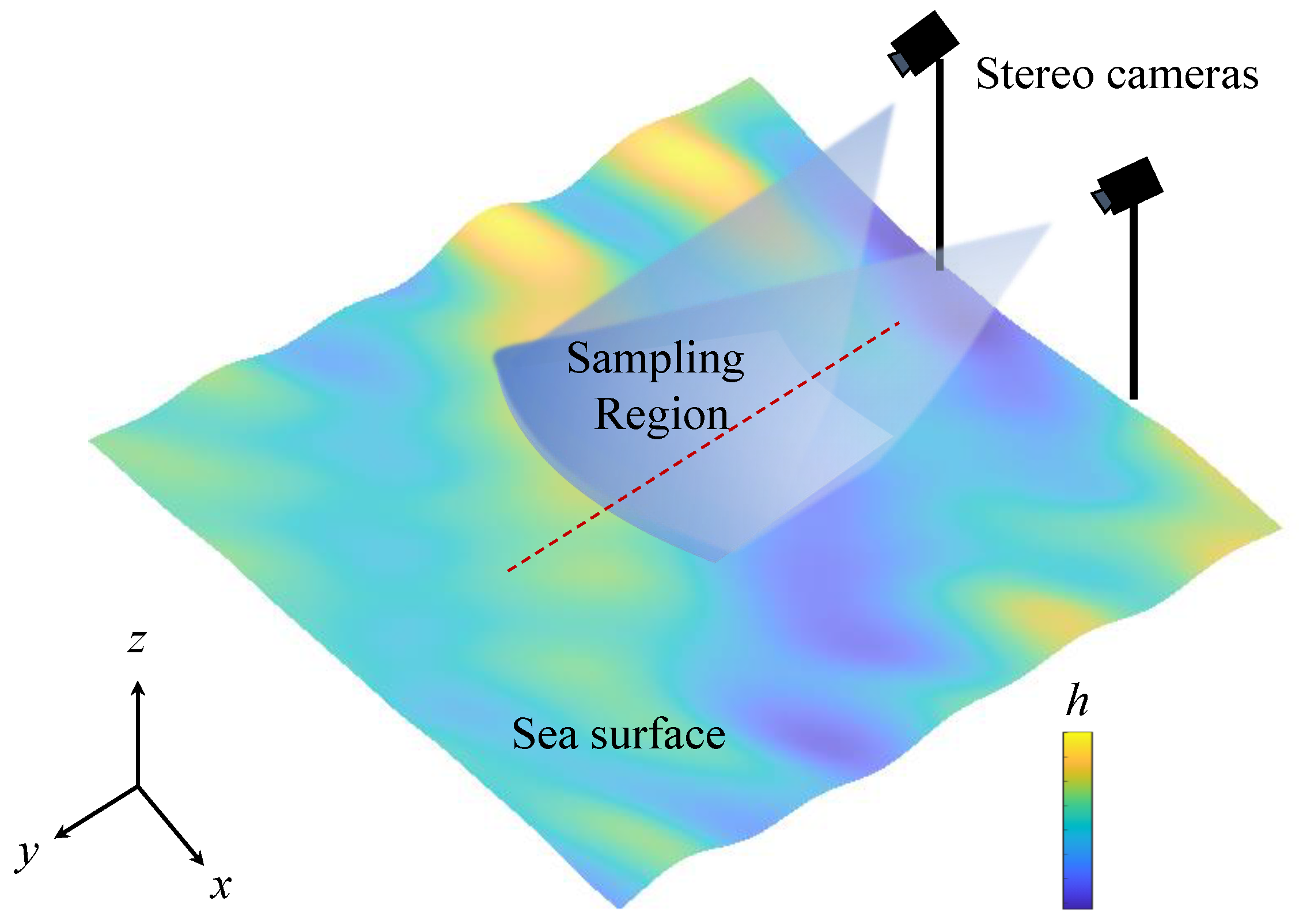
3. Experimental Design and Construction of Data Sets

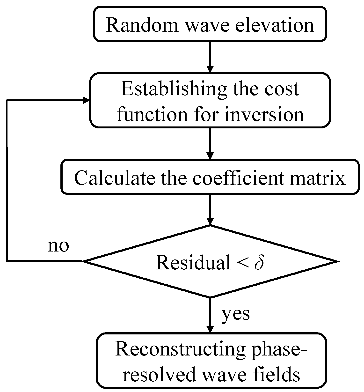
3.1. Phase-Resolved Wave Reconstruction Algorithms

With the methodology clearly outlined, we now focus on the experimental design and the processes involved in constructing the datasets for our study. To invert and reconstruct the phase-resolved wave field from the sampling point R m × 3 , we employ the linear wave theory (LWT) model. The overall flow of the reconstruction algorithm is shown in Figure 2, where A 0 is added as the random initial condition. Then, we calculate the coefficient matrix for the LWT model through iteration, with a convergence criterion δ = 1 × 10 6 .
We construct the LWT model by the Eulerian method for modeling rotation-free, noncohesive, incompressible fluids. A Cartesian coordinate system ( x , y , z ) is considered, with the x-axis and y-axis located at the horizontal water surface and the z-axis along the vertical direction. The linear superposition of n = 1 , . . . , N individual wave harmonics of amplitude A n , angular frequency ω n , and direction of propagation Θ n yields the linear ocean surface representation in the horizontal plane of coordinates r = ( x , y ) :
η lim r , t = n = 1 N A n cos k n · r ω n t φ n ,
where t is time, φ n = 2 π R n is mutually independent (i.e., random) phases, with R n [ 0 , 1 ] being a set of uniformly distributed random numbers. k n = k n k ^ n = k n cos θ n , k n sin θ n and k n = 2 π / λ n = | k n | are wave number vectors and wavenumbers. With the deep water dispersion relationship, wavenumbers are found as k n = ω n 2 / g , where g is the acceleration of gravity.
To simplify the following mathematical and algorithm developments related to free surface reconstruction, it is more convenient (and numerically accurate) to use the equivalent linear representation:
η lin r , t = n = 1 N a n cos ψ n + b n sin ψ n ,
where { a n , b n ; n = 1 , , N } are 2 N wave harmonic parameters describing the ocean surface, with ( a n , b n ) = A n cos φ n , A n sin φ n , and ψ n = k n · r ω n t are spatio-temporal phases.
We invert the wave parameters based on a linear wave model to perform the sea surface reconstruction. The standard approach to wave reconstruction based on observed data is the variational approach [14], which optimizes the values of 2 N unknown parameters ( a n , b n ) by minimizing the root-mean-square (RMS) difference between the wave observations and their model representation. Thus, the cost function is defined as
F ( p ) = 1 2 l = 1 L ( η ( p ) η l ) 2 ,
where p = a n , b n ( n = 1 , , N ) is the control vector of 2 N unknown model parameters, η ( p ) is the unknown reconstructed sea surface elevation computed by the linear wave model (an given in Equation (14)), and η l ( l = 1 , , L ) is the point cloud elevation obtained from downsampled observations.
The model parameters are obtained by minimizing the cost function and solving the system of equations:
F a m = 0 , F b m = 0 ,
where m [ 1 , . . . , N ] .
Developing these equations yields a linear system of 2 N equations for 2 N unknown parameters:
l = 1 L n = 1 N { a n cos ψ m l cos ψ n l + b n cos ψ m l sin ψ n l } = l = 1 L η l cos ψ m l , l = 1 L n = 1 N { a n sin ψ m l cos ψ n l + b n sin ψ m l sin ψ n l } = l = 1 L η l sin ψ m l ,
where wave harmonic phases are defined as ψ m l = k m · r l ω m t l .
Rewrite Equation (18) in matrix form as:
A m n p n = B m ,
where p n is a vector made of the 2 N unknown parameters p n = a n , p N + n = b n , and A is the 2 N × 2 N matrix given by:
A = [ A m n , A m , N + n ; A N + m , n , A N + m , N + n ] , A m n = = 1 L cos ψ n cos ψ m , A m , N + n = = 1 L sin ψ n cos ψ m , A N + m , n = = 1 L cos ψ n sin ψ m , A N + m , N + n = = 1 L sin ψ n sin ψ m ,
and B is the 1 × 2 N vector given by:
B = [ B m , B N + m ] , B m = = 1 L η cos ψ m , B N + m = = 1 L η sin ψ m .
When inverting waves in the observation area, especially short-peak waves, the condition number of the A matrix is often huge, making the inversion problem often pathological. To address this, we apply Tikhonov regularization, which yields consistent solutions by minimizing the approximated error function:
min A m n p n B n 2 ξ 2 p n 2 ,
where ξ is the regularization parameter, which is selected by generalized cross-validation (GCV), which minimizes the error in the post-test unit weights, i.e., maximizes the confidence in the observations from which the GCV function is constructed. When the GCV function achieves the minimum value, the corresponding ξ is the regularization parameter. After solving for the wave parameters, we can reconstruct the phase-resolved wave field z r , which is used to calculate the task loss in Equation (13).

3.2. Constructing Datasets

In this work, the origin point cloud is measured by stereo cameras installed on the ship. To illustrate this process and verify the effectiveness of our framework, we first construct a data set from the numerical sea wave based on the LWT model. Figure 3 shows the sampling process by stereo cameras, which face downward at an angle of 45° along the negative direction of the z-axis. The horizontal aperture angle of the cameras is 70° and the vertical aperture angle is 55°. The stereo camera captures 32,468 pixel pairs in the viewing range. Three-dimensional coordinates of the point cloud are intersection points between the rays and waves’ surface.
We construct random waves in the horizontal coordinate range ( x , y ) [ 128 , 128 ] meters and the PM wave spectrum. The specific form of the spectrum is as follows:
S ( ω ) = 0.78 ω 5 exp [ 5 4 ( 0.795 ω ) 4 ] 2 π cos 2 θ ,
where ω is the frequency of the component wave and θ is the direction of the component wave. The coordinates are the wave’s three-dimensional coordinates ( x , y , z ) in meters at the observation point, where z represents the wave elevation. We generate 2000 random wave samples in Matlab, using 1400 for training, 350 for validation, and 350 for testing. A single point cloud consists of 32,468 points.
Next, we obtain dense point cloud data from the stereo observation images of waves using the WASS method. This wave stereo 3D reconstruction pipeline is shown in Figure 4. Sextant’s publicly available YS 01 wave stereo image data were used as the input for the open-source project [52]. The dataset consists of three-dimensional wavelengths observed during the passage of atmospheric fronts, which is applicable to this study since the phenomenon results in a broad directional propagation of wave energy.
The reconstruction of the wave point cloud using the WASS method in this work is divided into three main steps: (i) Feature extraction and matching: The input stereo image is subjected to feature extraction and matching. Following this, the rotation and translation matrices are computed. (ii) Rectification: the extrinsic and intrinsic calibration data are used to rectify the two stereo images. (iii) Disparity map and point cloud generation: After rectification, a dense stereo algorithm obtains the disparity map between the two frames. Preliminary morphological filters are then applied directly to the disparity map. The initial unfiltered 3D point cloud is generated by triangulating the corresponding pixels. Points with outlier depths and those not belonging to the most significant connected component are filtered out.
An initial robust RANSAC estimation of the mean plane is performed [53]. The algorithm fits the model by continuously randomly sampling a subset of the data and then determining the inlier points based on a threshold of the residuals. This process is repeated to obtain the optimal planar model with the maximum number of inlier points:
a x + b y + c z + d = 0 ,
where ( a , b , c ) is the normal vector n 1 to the plane and d is the intercept to the origin.
The goal is to rotate the initial plane to be parallel to the z-axis (i.e., horizontal) with an average vector of n 2 = [ 0 , 0 , 1 ] . We must compute a rotation matrix Γ such that R × n 1 = n 2 . Compute the axis of rotation as the cross product of the two vectors u = n 1 n 2 . Compute the angle of rotation θ as the angle between the two vectors. Use the Rodrigues’ rotation formula to calculate the rotation matrix Γ :
Γ = I + sin ( θ ) · [ u ] × + ( 1 cos ( θ ) ) · [ u ] × 2 ,
where [ u ] × is the antisymmetric matrix of vector u. The translation vector is calculated by T = n 1 n 2 . The final coordinate transformation of the original point cloud P is based on the rotation matrix Γ and the translation vector T. The transformed coordinate P can be calculated by the following equation:
P = Γ · P + T ,
The WASS method acquires a 3D point cloud of ocean waves at the 10 5 level of data, which is too large for a neural network. After experiments, compressing the number of point clouds to one-tenth can guarantee a more than 95 % reconstruction integrity ratio. To balance performance and computational efficiency, we used the farthest point sampling (FPS) method to sample the data of a single point cloud up to 32,468 points. After performing the above pre-processing operations on 2000 WASS-extracted 3D point cloud data of actual ocean waves, we took 1400 point cloud samples as a training set, 350 as a validation set, and 350 as a test set.
Our proposed downsampling network is first trained and evaluated using a simulated ocean wave dataset. We use a server with an NVIDIA GeForce RTX 2080 TI GPU for training, with a batch size set to 8, epochs set to 400, bottleneck size to 128, and output points set to 512. We use an Adam optimizer with an initial learning rate of 0.001. To ensure the uniformity of sampling, we compress each point cloud into a unit voxel for sampling and recover the original and sampled point cloud sizes to calculate the task loss when reconstructing the task.

4. Experimental Results and Discussion

With the experimental design and dataset construction methods in place, we first verify the effectiveness of our algorithm by using the simulated wave and then evaluate the performance on actual sea wave cases in this section. The objective is to obtain an optimal sampling strategy with a low sampling ratio and to analyze the underlying mechanisms.

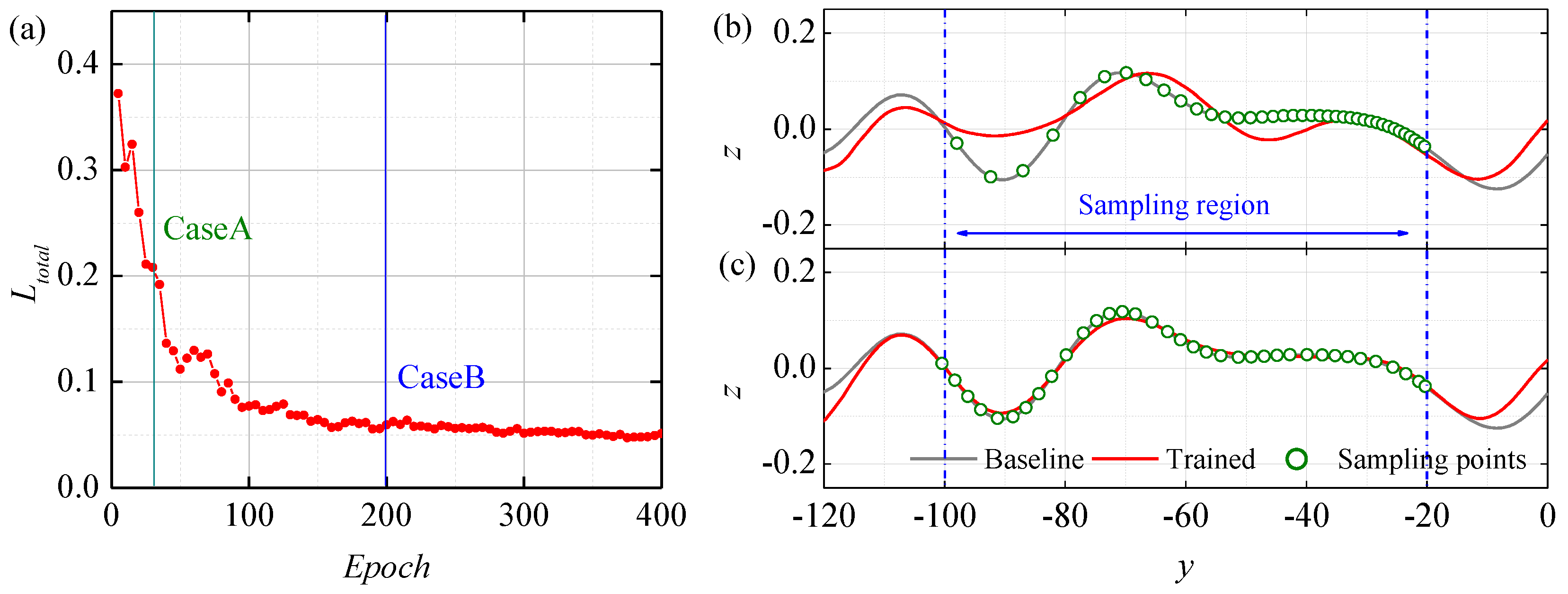
4.1. Training and Evaluation Based on Simulated Wave Datasets

Figure 5a displays the evolution of total loss L t o t a l during the training. L t o t a l converges with an approximately exponential decay trend as the number of training epochs increases. After 200 training epochs, the losses approximately converge. Total loss decreased from an initial value of 0.37 to 0.05 at E p o c h = 400 , which improves the performance of the downstream reconstruction task by 32%. To illustrate the sampling results and reconstruction effects of the network, we select two snapshots during training, that is CaseA ( E p o c h = 30 ) and CaseB ( E p o c h = 200 ) in Figure 5a. We present the one-dimensional wave cross-section form ( x , y ) = ( 0 , 0 ) to ( x , y ) = ( 0 , 120 ) (red line shown in Figure 3).
Figure 5b shows observation points are not uniform in spatial distribution, which is denser for closer to the location of the camera and relatively sparse for those far away. Before optimizing the sampling strategy, the distribution of the sampling points was similar to that of the original observation point. Since the wave reconstruction effect of the downstream task is determined by the distribution of sampling points, it can be intuitively deduced from the figure that this sampling result would lead to an increase in reconstruction error with increasing distance from the camera. Figure 5c shows that the optimized sampling points are more uniformly distributed, and no longer densely clustered near the camera but evenly spread across the entire sampling area. The uniformly distributed sampling points can better reproduce the overall wave shape, avoiding the previous situation where the reconstruction quality was higher near the camera and lower in farther areas. The reconstruction effect curve shows that the trained network can predict the wavefront more accurately in the observation area, and the reconstruction error remains stable across the entire sampling area without exhibiting a rapid increase with increasing distance. Figure 6 shows the inversion results after training at different wavelengths and directions. We can reach the same conclusion as shown in Figure 5c, which validates that our method is robust for wave inversion on different wavelengths and angle spreads.
Then, we evaluate the impact of the proposed sampling strategy optimization method on the reconstructed wave contour map. To evolute the performance of our method, we define the spatial residuals between the reconstructed results and origin wave data as:
R e s = | z r z t | z r , with ( z r , z t ) ( x , y ) ,
where z r and z t are the height of reconstructed wave and origin wave fields, respectively. Figure 7a shows the original natural wave contour map as a benchmark comparison. Figure 7b presents the reconstruction results before training the sampling network. The reconstruction results are relatively accurate when close to the observation area (i.e., the location of the camera). However, the reconstruction accuracy decreases sharply with the increasing distance. There are apparent distortions and aberrations in the waveforms far from the observation area. This phenomenon is consistent with our previous analysis of the problem caused by the uneven distribution of sampling points.
In contrast, Figure 7c shows the reconstruction results after training with the optimized sampling strategy. After learning, the network output sampling points became more uniform, significantly improving the quality of the reconstructed contour maps over the entire observation area (both near and far from the observation area). The distribution of the peaks and troughs is more precise, with no severe distortion or flattening. To quantitatively evaluate the errors, the relative errors between the reconstruction results in Figure 7c and the original wave contours in Figure 7a are visualized in Figure 7d. From the error distribution, the reconstruction errors are controlled at a low level in 90 % of the observed area, verifying that our method effectively improves the problem of degradation in reconstruction accuracy caused by the uneven distribution of sampling points.

4.2. Training and Evaluation Based on Real Wave Data Set

The above experimental results validate the effectiveness of our proposed deep learning-based adaptive sampling policy network. To address the more complex features and details of the natural wave dataset, we improve and optimize the PointNet-based network architecture. We increase the number of channels/neurons in the convolutional and fully connected layers. For example, the output channels of the first convolutional layer increase from 64 to 128, and the output dimensions of the last fully connected layer increase from 256 to 512. Moreover, a batch normalization layer is added after each convolutional and fully connected layer to accelerate the training convergence and improve the model’s generalization ability. Although we retain the basic encoder–decoder framework of the PointNet, the depth of the network is appropriately adjusted by increasing the number of fully connected layers from 2 to 3. This adjustment enables the network to perform deeper feature extraction and fusion.
Our propose is obtaining a high completeness ratio C R between the reconstructed wave and real wave by a sampling strategy with as few as sampling points. Then, we define sampling ratio as:
S R = log 2 N s N t ,
where N t = 2 15 is the number of total sampling point from WASS, and N s is the number we used. We introduce two other methods as a comparison, the FPS method and random sampling algorithms, to evaluate the performance of the present method. As shown in Figure 8, C R increases with the increases in S R for all three methods, and the sampling network keeps the leading position followed by the FPS method. For low sampling ratios S R [ 9 , 7 ] , FPS and random sampling algorithms have poorer reconstruction results ( C R < 0.5 ). However, our sampling network shows excellent ability in these ranges; for example, the completeness ratio can reaches 0.78 more than 37 % compared the FPS method ( C R = 0.43 ) at S R = −7. When S R = −6, our method can reach C R = 0.91 , which leads the reconstruction task performance by more than 30 % compared other two methods. In the higher sampling interval S R [ 4 , 2 ] , the performance gap between the three methods narrows. However, our method maintains a slight lead throughout the interval, consistently achieving a 1–2% higher C R than the traditional methods. This highlights the superior performance of the algorithm in various sampling density scenarios for the downstream reconstruction task.
We chose three different sampling ratios S R = 8 , −6, and −5 and observed the convergence process of their training. As shown in Figure 9, the total loss in all three cases shows a decaying trend with the number of training epochs. For the case of S R = −8, the reconstruction task performance improves by 24% at the end of training. However, the number of points is too small to capture the small-scale wave features, leading to only the main wave information being extracted. When increasing the sampling ratios to S R = −6 and −5, we observe that these two cases share similar convergence curves. The main difference is that the error for S R = −5 converges slightly faster in the initial training phase. To balance the sampling density and the computational efficiency, we select the case of S R = −6 for subsequent analyses.
Figure 9 illustrates the spatial distribution of sampling points from the global views (the first row) and the horizontal projections (the second row). To better present the distribution of the point cloud during the training process, we chose one point for every five neighboring points to show the distribution. The distribution of sampling points during the pre-training phase (Phase-I in Figure 9) is notably uneven, as shown in Figure 10a1,a2. Most sampling points are concentrated in the central region of the observation frame and in proximity to the observation viewpoint. Conversely, sampling points are relatively sparse in the peripheral regions, away from the viewpoint along the frame’s edges. This inhomogeneous distribution arises from inherent variations in the density of the original point cloud data across different regions. Figure 10b1,b2. depicts the distribution of sampling points during Phase-II. Compared to Phase-I, the sampled points exhibit a more uniform distribution throughout the observation area, with a reduction in the density of the central region and an increase in the number of points in the edge regions, albeit with some residual sparse areas. Figure 10c1,c2. presents the final distribution of sampling points in the post-training stage (Phase-III). Following comprehensive network optimization, the sampling points demonstrate a uniform and random distribution in three-dimensional space, no longer exhibiting excessive concentration in specific regions. Both central and peripheral areas exhibit balanced densities without any conspicuous blank or overdense regions. The adaptive sampling algorithm’s gradual optimization of the sampling strategy during the training process transforms the initially uneven distribution, influenced by the observation viewpoint, into a final optimized sampling distribution that uniformly and efficiently covers the entire area.
Figure 11a illustrates the spatial residuals R e s in Phase-I, where dark regions are apparent in the residual plot, indicating significant discrepancies between the reconstruction results and the actual data. The highest residual values and poorest reconstruction quality are observed in the peripheral regions furthest from the observing system. In these regions, the density of the original point cloud data are low, resulting in sparse sampling points and posing substantial challenges for the subsequent reconstruction process. In contrast, the central region near the observation viewpoint exhibits superior reconstruction quality due to the high density and more uniform distribution of the sampling points. Figure 11b corresponds to the residual map during the mid-training stage. Compared to the initial state, the residual distribution exhibits a significant improvement. Nonetheless, high residual values persist in the edge regions distant from the observation viewpoint, indicating a need for further enhancement of the reconstruction quality. Figure 11c presents the final residual distribution at the post-training stage. Notably, both the central and peripheral areas show an almost complete absence of dark regions in the residual map, with the entire area displaying a light gray hue and residual values being exceptionally close to zero.
This observation indicates that, after sufficient training, our algorithm can accurately reconstruct the wave structure, closely approximating the natural wave structure and effectively mitigating the reconstruction errors induced by the initial uneven distribution of the sampling points. The residuals have been minimized. By comparing the residual plots across different training stages, we observe a substantial improvement in the algorithm’s reconstruction accuracy after undergoing learning and optimization, particularly in the edge areas where reconstruction quality was initially compromised due to the sparse point cloud. Post-training, these areas exhibit significant enhancement, validating the high reconstruction quality and reliability of our algorithm.

5. Conclusions

In this work, we develop a phase-resolved wave field reconstruction method by the learning-based downsampling network to handle ocean wave data obtained by optical systems. To do this, we first extract dense point clouds from ocean wave snapshots using WASS. Then, we couple learning-based downsampling networks with the phase-resolved wave reconstruction algorithm, training them to improve the wave reconstruction completeness ratio C R . Next, we test the performance of our algorithm on numerical ocean waves modeled by the liner wave theory model. Results indicate that the trained sampling network leads a more uniform spatial distribution of sampling points and improves C R at the observed edge regions far from the camera. Finally, we apply our algorithm to a natural ocean wave dataset. It can improve the averaged completeness ratio over 30% at low sampling ratios ( S R [ 2 9 , 2 7 ] ) compared to the traditional FPS method and Random sampling method. Additionally, the relative residual between the final reconstructed wave and the natural wave is less than 15%.
Our algorithm enables fast and real-time phase-resolved wave field reconstruction in partial ocean engineering applications. In the future, this algorithm could play a significant role in short-term deterministic sea wave prediction (DSWP) and real-time analysis of wave loads. Moreover, it paves the way for developing new inversion algorithms, such as discrete Fourier transform, for wave reconstruction. This could further be applied to autonomous vessel trajectory tracking and path optimization, optimization of marine equipment, and safety analysis of maritime operations, providing possibilities for the intelligent development of the ocean engineering field.

Author Contributions

T.M.: Conceptualization (lead); Formal analysis (lead); Investigation (lead); Methodology (lead); Validation (lead); Visualization (lead); Writing—original draft (lead); Writing—review and editing (equal). Z.S.: Supervision (lead); Writing—review and editing (equal). G.X.: Formal analysis (equal). All authors have read and agreed to the published version of the manuscript.

Funding

This work is supported by the National Natural Science Foundation of China (grant No. 51879027).

Data Availability Statement

No new data were created or analyzed in this study. Data sharing is not applicable to this article.

Conflicts of Interest

The authors declare no conflicts of interest.

References

  1. Li, G.; Weiss, G.; Mueller, M.; Townley, S.; Belmont, M.R. Wave energy converter control by wave prediction and dynamic programming. Renew. Energy 2012, 48, 392–403. [Google Scholar] [CrossRef]
  2. Ma, Y.; Sclavounos, P.D.; Cross-Whiter, J.; Arora, D. Wave forecast and its application to the optimal control of offshore floating wind turbine for load mitigation. Renew. Energy 2018, 128, 163–176. [Google Scholar] [CrossRef]
  3. Kusters, J.G.; Cockrell, K.L.; Connell, B.S.H.; Rudzinsky, J.P.; Vinciullo, V.J. FutureWaves™: A Real-Time Ship Motion Forecasting System employing Advanced Wave-Sensing Radar. In Proceedings of the OCEANS 2016 MTS/IEEE Monterey, Monterey, CA, USA, 19–23 September 2016. [Google Scholar] [CrossRef]
  4. Jiang, H.K.; Zhang, Y.; Zhang, Z.Y.; Luo, K.; Yi, H.L. Instability and bifurcations of electro-thermo-convection in a tilted square cavity filled with dielectric liquid. Phys. Fluids 2022, 34, 064116. [Google Scholar] [CrossRef]
  5. Rajendran, S.; Fonseca, N.; Guedes Soares, C.; Clauss, G.n.F.; Klein, M. Time domain comparison with experiments for ship motions and structural loads on a container ship in abnormal waves. In Proceedings of the International Conference on Offshore Mechanics and Arctic Engineering, Rotterdam, The Netherlands, 19–24 June 2011; Volume 44380, pp. 919–927. [Google Scholar]
  6. Kim, I.C.; Ducrozet, G.; Perignon, Y. Development of phase-resolved real-time wave forecasting with unidirectional and multidirectional seas. In Proceedings of the International Conference on Offshore Mechanics and Arctic Engineering, Boston, MA, USA, 20–23 August 2023; American Society of Mechanical Engineers: Boston, MA, USA, 2023; Volume 86878, p. V005T06A104. [Google Scholar]
  7. Abusedra, L.; Belmont, M. Prediction diagrams for deterministic sea wave prediction and the introduction of the data extension prediction method. Int. Shipbuild. Prog. 2011, 58, 59–81. [Google Scholar]
  8. Naaijen, P.; Huijsmans, R. Real time wave forecasting for real time ship motion predictions. In Proceedings of the International Conference on Offshore Mechanics and Arctic Engineering, Estoril, Portugal, 15–20 June 2008; Volume 48210, pp. 607–614. [Google Scholar]
  9. Nguyen, H.N.; Tona, P. Short-term wave force prediction for wave energy converter control. Control Eng. Pract. 2018, 75, 26–37. [Google Scholar] [CrossRef]
  10. Nguyen, H.N.; Tona, P. Wave excitation force estimation for wave energy converters of the point-absorber type. IEEE Trans. Control Syst. Technol. 2017, 26, 2173–2181. [Google Scholar] [CrossRef]
  11. Kim, I.C.; Ducrozet, G.; Leroy, V.; Bonnefoy, F.; Perignon, Y.; Delacroix, S. Numerical and experimental investigation on deterministic prediction of ocean surface wave and wave excitation force. Appl. Ocean Res. 2024, 142, 103834. [Google Scholar] [CrossRef]
  12. Desmars, N.; Hartmann, M.; Behrendt, J.; Hoffmann, N.; Klein, M. Nonlinear deterministic reconstruction and prediction of remotely measured ocean surface waves. J. Fluid Mech. 2023, 975, A8. [Google Scholar] [CrossRef]
  13. Zhang, Z.; Tang, T.; Li, Y. Spatial estimation of unidirectional wave evolution based on ensemble data assimilation. Eur. J.-Mech.-B/Fluids 2024, 106, 1–12. [Google Scholar] [CrossRef]
  14. Desmars, N.; Bonnefoy, F.; Grilli, S.T.; Ducrozet, G.; Perignon, Y.; Guérin, C.A.; Ferrant, P. Experimental and numerical assessment of deterministic nonlinear ocean waves prediction algorithms using non-uniformly sampled wave gauges. Ocean Eng. 2020, 212, 107659. [Google Scholar] [CrossRef]
  15. Jiang, H.K.; Luo, K.; Zhang, Z.Y.; Wu, J.; Yi, H.L. Global linear instability analysis of thermal convective flow using the linearized lattice Boltzmann method. J. Fluid Mech. 2022, 944, A31. [Google Scholar] [CrossRef]
  16. Simpson, A.; Haller, M.; Walker, D.; Lynett, P.; Honegger, D. Wave-by-wave forecasting via assimilation of marine radar data. J. Atmos. Ocean. Technol. 2020, 37, 1269–1288. [Google Scholar] [CrossRef]
  17. Bruneton, E.; Neyret, F.; Holzschuch, N. Real-time realistic ocean lighting using seamless transitions from geometry to BRDF. Comput. Graph. Forum 2010, 29, 487–496. [Google Scholar] [CrossRef]
  18. Babanin, A.V.; Soloviev, Y.P. Variability of directional spectra of wind-generated waves, studied by means of wave staff arrays. Mar. Freshw. Res. 1998, 49, 89–101. [Google Scholar] [CrossRef]
  19. Nwogu, O. Maximum entropy estimation of directional wave spectra from an array of wave probes. Appl. Ocean Res. 1989, 11, 176–182. [Google Scholar] [CrossRef]
  20. Luo, K.; Jiang, H.K.; Wu, J.; Zhang, M.; Yi, H.L. Stability and bifurcation of annular electro-thermo-convection. J. Fluid Mech. 2023, 966, A13. [Google Scholar] [CrossRef]
  21. Vogelzang, J.; Boogaard, K.; Reichert, K.; Hessner, K. Wave height measurements with navigation radar. Int. Arch. Photogramm. Remote Sens. 2000, 33, 1652–1659. [Google Scholar]
  22. Irish, J.L.; Wozencraft, J.M.; Cunningham, A.G.; Giroud, C. Nonintrusive measurement of ocean waves: Lidar wave gauge. J. Atmos. Ocean. Technol. 2006, 23, 1559–1572. [Google Scholar] [CrossRef]
  23. Brock, J.C.; Purkis, S.J. The emerging role of lidar remote sensing in coastal research and resource management. J. Coast. Res. 2009, 53, 1–5. [Google Scholar] [CrossRef]
  24. Kabel, T.; Georgakis, C.T.; Zeeberg, A.R. Mapping ocean waves using new lidar equipment. In Proceedings of the ISOPE International Ocean and Polar Engineering Conference, Honolulu, HI, USA, 16–21 June 2019. [Google Scholar]
  25. Evans, A. Laser scanning applied to hydraulic modeling. In Proceedings of the International Archives of Photogrammetry, Remote Sensing and Spatial Information Sciences, Commission V Symposium, Hong Kong, China, 26–28 May 2010. [Google Scholar]
  26. Shemdin, O.H.; Tran, H.M.; Wu, S. Directional measurement of short ocean waves with stereophotography. J. Geophys. Res. Ocean. 1988, 93, 13891–13901. [Google Scholar] [CrossRef]
  27. Kim, I.C.; Ducrozet, G.; Bonnefoy, F.; Leroy, V.; Perignon, Y. Real-time phase-resolved ocean wave prediction in directional wave fields: Enhanced algorithm and experimental validation. Ocean Eng. 2023, 276, 114212. [Google Scholar] [CrossRef]
  28. Belmont, M. Wave shadowing effects on phase resolved wave spectra estimated from radar backscatter: Part 1: An investigation of the errors due to wave shadowing in the spectral averaging approach. Ocean Eng. 2023, 267, 113409. [Google Scholar] [CrossRef]
  29. Xiao, Z.; Huang, W. Kd-tree based nonuniform simplification of 3D point cloud. In Proceedings of the 2009 Third International Conference on Genetic and Evolutionary Computing, Guilin, China, 14–17 October 2009; pp. 339–342. [Google Scholar]
  30. Eldar, Y.; Lindenbaum, M.; Porat, M.; Zeevi, Y.Y. The farthest point strategy for progressive image sampling. IEEE Trans. Image Process. 1997, 6, 1305–1315. [Google Scholar] [CrossRef] [PubMed]
  31. Luebke, D.P. A developer’s survey of polygonal simplification algorithms. IEEE Comput. Graph. Appl. 2001, 21, 24–35. [Google Scholar] [CrossRef]
  32. Quach, M.; Pang, J.; Tian, D.; Valenzise, G.; Dufaux, F. Survey on deep learning-based point cloud compression. Front. Signal Process. 2022, 2, 846972. [Google Scholar] [CrossRef]
  33. Shi, B.Q.; Liang, J.; Liu, Q. Adaptive simplification of point cloud using k-means clustering. Comput.-Aided Des. 2011, 43, 910–922. [Google Scholar] [CrossRef]
  34. Benhabiles, H.; Aubreton, O.; Barki, H.; Tabia, H. Fast simplification with sharp feature preserving for 3D point clouds. In Proceedings of the 2013 11th international symposium on programming and systems (ISPS), Algiers, Algeria, 22–24 April 2013; pp. 47–52. [Google Scholar]
  35. Alexiou, E.; Tung, K.; Ebrahimi, T. Towards neural network approaches for point cloud compression. In Proceedings of the SPIE Applications of Digital Image Processing XLIII, Online, 24 August–4 September 2020; Volume 11510, pp. 18–37. [Google Scholar]
  36. Qian, Y.; Hou, J.; Zhang, Q.; Zeng, Y.; Kwong, S.; He, Y. Mops-net: A matrix optimization-driven network fortask-oriented 3d point cloud downsampling. arXiv 2020, arXiv:2005.00383. [Google Scholar]
  37. Cheng, T.Y.; Hu, Q.; Xie, Q.; Trigoni, N.; Markham, A. Meta-sampler: Almost-universal yet task-oriented sampling for point clouds. In Proceedings of the European Conference on Computer Vision, Tel Aviv, Israel, 23–27 October 2022; pp. 694–710. [Google Scholar]
  38. Hong, C.Y.; Chou, Y.Y.; Liu, T.L. Attention discriminant sampling for point clouds. In Proceedings of the IEEE/CVF International Conference on Computer Vision, Paris, France, 2–6 October 2023; pp. 14429–14440. [Google Scholar]
  39. Dovrat, O.; Lang, I.; Avidan, S. Learning to sample. In Proceedings of the IEEE/CVF Conference on Computer Vision and Pattern Recognition, Long Beach, CA, USA, 15–20 June 2019; pp. 2760–2769. [Google Scholar]
  40. Ye, Y.; Yang, X.; Ji, S. APSNet: Attention based point cloud sampling. arXiv 2022, arXiv:2210.05638. [Google Scholar]
  41. Wang, X.; Jin, Y.; Cen, Y.; Wang, T.; Tang, B.; Li, Y. Lightn: Light-weight transformer network for performance-overhead tradeoff in point cloud downsampling. arXiv 2023, arXiv:2202.06263. [Google Scholar] [CrossRef]
  42. Lin, C.; Li, C.; Liu, Y.; Chen, N.; Choi, Y.K.; Wang, W. Point2skeleton: Learning skeletal representations from point clouds. In Proceedings of the IEEE/CVF Conference on Computer Vision and Pattern Recognition, Virtual, 19–25 June 2021; pp. 4277–4286. [Google Scholar]
  43. Wen, C.; Yu, B.; Tao, D. Learnable skeleton-aware 3d point cloud sampling. In Proceedings of the IEEE/CVF Conference on Computer Vision and Pattern Recognition, Vancouver, BC, Canada, 17–24 June 2023; pp. 17671–17681. [Google Scholar]
  44. Zhang, G.; Zhao, W.; Liu, J.; Liu, X. REPS: Reconstruction-based Point Cloud Sampling. arXiv 2024, arXiv:2403.05047. [Google Scholar]
  45. Makarynskyy, O. Neural pattern recognition and prediction for wind wave data assimilation. Pac Ocean. 2005, 3, 76–85. [Google Scholar]
  46. Fringer, O.B.; Dawson, C.N.; He, R.; Ralston, D.K.; Zhang, Y.J. The future of coastal and estuarine modeling: Findings from a workshop. Ocean Model. 2019, 143, 101458. [Google Scholar] [CrossRef]
  47. Parker, K.; Hill, D. Evaluation of bias correction methods for wave modeling output. Ocean Model. 2017, 110, 52–65. [Google Scholar] [CrossRef]
  48. Ellenson, A.; Pei, Y.; Wilson, G.; Özkan-Haller, H.T.; Fern, X. An application of a machine learning algorithm to determine and describe error patterns within wave model output. Coast. Eng. 2020, 157, 103595. [Google Scholar] [CrossRef]
  49. Wang, N.; Chen, Q.; Zhu, L.; Sun, H. Integration of data-driven and physics-based modeling of wind waves in a shallow estuary. Ocean Model. 2022, 172, 101978. [Google Scholar] [CrossRef]
  50. Wang, N.; Chen, Q.; Chen, Z. Reconstruction of nearshore wave fields based on physics-informed neural networks. Coast. Eng. 2022, 176, 104167. [Google Scholar] [CrossRef]
  51. Bergamasco, F.; Torsello, A.; Sclavo, M.; Barbariol, F.; Benetazzo, A. WASS: An open-source pipeline for 3D stereo reconstruction of ocean waves. Comput. Geosci. 2017, 107, 28–36. [Google Scholar] [CrossRef]
  52. Guimarães, P.V.; Ardhuin, F.; Bergamasco, F.; Leckler, F.; Filipot, J.F.; Shim, J.S.; Dulov, V.; Benetazzo, A. A data set of sea surface stereo images to resolve space-time wave fields. Sci. Data 2020, 7, 145. [Google Scholar] [CrossRef]
  53. Fischler, M.A.; Bolles, R.C. Random sample consensus: A paradigm for model fitting with applications to image analysis and automated cartography. Commun. ACM 1981, 24, 381–395. [Google Scholar] [CrossRef]
Figure 1. Overview structure of the network.
Jmse 12 01082 g001
Figure 2. Algorithm loop for the reconstruction of the phase-resolved wave field.
Jmse 12 01082 g002
Figure 3. Diagram of the sampling process by stereo cameras. Grey region is the sampling region.
Jmse 12 01082 g003
Figure 4. Point cloud construction by WASS. (a) is a stereo image. (b) shows the sea wave after matching. (c) is the rectification process. (d) is the reconstructed wave point cloud.
Jmse 12 01082 g004
Figure 5. (a) Time evolution of L t o t a l with the Epoch during training process; (b,c) are a comparison between the real ocean wave and the reconstructed result for CaseA and CaseB at ψ = 0 in (a), respectively.
Jmse 12 01082 g005
Figure 6. A comparison between the real ocean wave and the reconstructed result for (a) ψ = 30 and (b) ψ = 0 .
Jmse 12 01082 g006
Figure 7. (a) is the origin ocean wave in a range of ( x , y ) [ 100 , 20 ] × [ 40 , 40 ] . (b,c) are the results before and after training, respectively. (d) shows a Res between the origin and trained ocean wave. Origin dots represents the range of the camera.
Jmse 12 01082 g007
Figure 8. The variation between the sampling ratio and completeness ratio of my present method compared with that of FPS and Random results.
Jmse 12 01082 g008
Figure 9. Total loss L t o t a l varies with the training epochs for sampling ratios S R = 8 , −6 and −5. Lines represent the average value and shadow region regions are deviation. Phase-I to -III are three phases during training for S R = −6 case.
Jmse 12 01082 g009
Figure 10. Spatial distribution of point cloud for (a1,a2) before train (Phase-I), (b1,b2) during training (Phase-II), and (c1,c2) after training (Phase-III). We plot 1 / 5 points for a clearer view.
Jmse 12 01082 g010
Figure 11. Spatial distribution of residual between the real ocean wave and reconstructed ocean wave (a) before training, (b) during training, and (c) after training.
Jmse 12 01082 g011
Disclaimer/Publisher’s Note: The statements, opinions and data contained in all publications are solely those of the individual author(s) and contributor(s) and not of MDPI and/or the editor(s). MDPI and/or the editor(s) disclaim responsibility for any injury to people or property resulting from any ideas, methods, instructions or products referred to in the content.

