Empirical Orthogonal Function Analysis on Long-Term Profile Evolution of Tidal Flats along a Curved Coast in the Qiantang River Estuary, China

Abstract

Abstract: Tidal flats are dynamic coastal ecosystems continually reshaped by natural processes and human activities. This study investigates the application of Empirical Orthogonal Function (EOF) analysis to the long-term profile evolution of tidal flats along the Jiansan Bend of the Qiantang River Estuary, China. By applying EOF analysis to profiles observed from 1984 to 2023, this study identifies dominant modes of variability and their spatial and temporal characteristics, offering insights into the complex sediment transport and morphological evolution processes. EOF analysis helps unravel the complex interactions between natural and anthropogenic factors shaping tidal flats, with the first three eigenfunctions accounting for over 90% of the observed variance. The first spatial eigenfunction captures the primary trend, while the subsequent two eigenfunctions reveal secondary and tertiary modes of variability. A conceptual model developed in this study elucidates the interplay between hydrodynamic forces and morphological changes, highlighting the rotation and oscillation of tidal flat profiles in response to seasonal variations in hydrological conditions. The findings emphasize the effectiveness of EOF analysis in capturing significant geomorphological processes and underscore its potential in enhancing the understanding of tidal flat dynamics, thereby informing more effective management and conservation strategies for these critical coastal environments.

1. Introduction

Tidal flats are highly dynamic and productive ecosystems situated at the junction of terrestrial and marine environments [1]. These areas, influenced by the ebb and flood of tides, play a crucial role in providing habitats for a wide variety of species [2], contribute significantly to coastal defense [3], and perform vital ecosystem services such as nutrient cycling and carbon sequestration [4,5]. However, their ever-changing profiles, molded by an interplay of sediment deposition, erosion, and biological activities [6], pose substantial challenges for monitoring and predicting future changes. These challenges are further compounded by the impacts of climate change [7,8], highlighting the need for advanced analytical techniques to understand and anticipate the evolution of tidal flats [9]. In particular, the curvature of certain coastal landscapes introduces additional variables into the complex dynamics that govern tidal flats.

The interaction between hydrodynamic forces and coastal morphology plays a significant role in shaping the characteristics of curved coasts [10], distinguishing them from straighter shorelines. These coasts experience a diverse range of hydrodynamic processes, including wave diffraction, refraction, and the convergence and divergence of tidal flows, all of which profoundly affect sediment transport and deposition patterns [11,12]. The Qiantang River Estuary (QRE), renowned for its dramatic tidal bores [13], serves as a prime example of such complexities. In this estuary, the curvature of the coast amplifies tidal ranges and alters current velocities, significantly affecting hydrodynamic conditions [14]. Therefore, studying the morphological evolution of tidal flats in these geomorphologically complex areas requires advanced analytical methods capable of dissecting the interactions between nature and anthropogenic factors. Among these methods, Empirical Orthogonal Function (EOF) analysis stands out for its ability to unravel the complex influences on the evolution of tidal flats [15,16,17], offering deep insights into the relationships between profile changes, tidal range, and runoff.

EOF analysis, also recognized as Principal Component Analysis within multivariate statistics, is an effective tool for identifying dominant modes of variability in complex datasets [18]. This analytical method has been widely adopted across various scientific domains, including meteorology, oceanography, and climatology [19], due to its proficiency in revealing patterns within noisy data. Initially introduced in the mid to late 1970s by research groups at the University of Virginia [20,21,22] and the Scripps Institute of Oceanography [23] in the United States, EOF analysis has significantly advanced coastal geomorphology and sedimentology research. Subsequent investigations have predominantly focused on sandy coastal topography and the dynamics of sediment influenced by wave actions [24,25]. These studies have detailed the spatiotemporal characteristics of surface sediments on the inner shelf, examined transport and exchange patterns of nearshore sediments [26,27], assessed the impacts of extreme weather events like storms and typhoons on beach terrains [28], and provided quantitative analyses of seasonal beach cycles [29,30] and human impacts [31,32,33]. In analyzing spatiotemporal changes in sandy coastal profiles, EOF is frequently integrated with other analytical methods [34], including spectral analysis [29], wavelet analysis [35], and canonical correlation analysis [36]. Such integrations enhance the examination of coastal equilibrium profiles [29], the understanding of typical geomorphological dynamic processes [37,38], the behavior of large-scale coastal systems [39], and the effectiveness of beach maintenance strategies [40].

While the majority of research has focused on sandy beaches, muddy and mixed sediment tidal flats have received less attention despite their significant ecological roles [41]. Muddy beaches, characterized by a complex array of developmental factors, display geomorphic features that are markedly distinct from those of sandy environments. The difficulty of field observations adds further challenges to collecting time-series data on tidal beach elevations that meet stringent analysis criteria [42]. Although the use of EOF analysis in studying the spatiotemporal dynamics of muddy coastal beaches has been limited, several studies have effectively applied this method to understand coastal zones along the northern shore of Hangzhou Bay and Jiangsu Coast in China [42]. Key studies include mapping seasonal variations of the tidal flat from Jinhuigang to Caojing [43], examining the development patterns of the Fangxian tidal flat [44], assessing morphological changes in the South Passage of the Changjiang estuary [45,46], and exploring the morphological evolution of the Jinshan trough [47]. Additionally, similar research in the Sittang River Estuary in Myanmar [48] indicates an increasing interest in using EOF analysis to analyze complex coastal systems.

Despite the valuable insights provided by EOF analysis and other integrated analytical techniques, research on tidal flat profiles encounters significant limitations. A primary issue is the lack of continuous, high-resolution data over extensive periods. Such data are essential to capture the subtle dynamics of tidal flats influenced by sediment supply, tidal dynamics, human activities, and climate change [31]. Furthermore, EOF analysis is effective in identifying variability patterns, but it relies on the assumption that data variance can be effectively decomposed into orthogonal components. However, this assumption may not always hold true in diverse coastal environments. This can lead to oversimplifications of complex environmental processes. Therefore, enhancing EOF analysis through integration with additional statistical techniques could significantly refine our understanding of tidal flat dynamics and evolution.

As depicted in Figure 1, the QRE is the largest macro-tidal estuary in China and connects to the East China Sea via Hangzhou Bay. The Jianshan Bend, located in the transitional section of the QRE, is influenced by both river runoffs and tidal flows. This area experiences significant changes due to erosion and sedimentation, and the main channel frequently shifts, displaying wandering characteristics. Since the 1950s, the Qiantang River Administration has conducted annual fixed cross-section observations of the QRE every April, July, and November. The Jianshan Bend, within the study area, features four observation profiles, providing a wealth of long-term data suitable for EOF analysis. However, curved river banks pose distinct challenges for EOF analysis due to their geometric complexity and the spatial variability of environmental factors. The curvature impacts tidal dynamics, wave propagation, and sediment transport pathways, leading to diverse morphological responses along the coastline. Consequently, EOF analysis of tidal flats along curved coastlines necessitates meticulous consideration of these spatial complexities to accurately delineate the processes driving profile evolution.

This study investigates the application of EOF analysis to the long-term profile evolution of tidal flats along curved coasts, a critically important yet under-researched topic. Our research aims to bridge this knowledge gap by using EOF analysis to examine the long-term evolution of tidal flat profiles along these coasts. This analysis seeks to identify the dominant modes of variability and the key factors influencing changes over time. Understanding these dynamics is essential for predicting future changes and informing conservation and management strategies for these vital coastal areas.

The paper is structured as follows: Section 1 provides a review of the literature on tidal flat dynamics and the use of EOF analysis in coastal geomorphology and sedimentology. Section 2 describes the methodology, including data collection, EOF analysis, and the integration of additional statistical methods. Section 3 presents the results of the EOF analysis, highlighting the dominant modes of variability and their spatial and temporal characteristics. Section 4 discusses the implications of these findings for enhancing our understanding of tidal flat evolution, addresses the limitations of the current study, and proposes directions for future research. Finally, Section 5 concludes with a summary of the key findings and suggestions for subsequent studies.

2. Materials and Methods

2.1. Study Area

The study site covers the western 12 km of the Jianshan Bend in the QRE, extending 8 km upstream and 4 km downstream from the Tashan Groin (Figure 2a). As depicted in Figure 1, the QRE is characterized by its trumpet-shaped estuary. Approximately 160 km upstream from the study area lies the Fuchun River Power Station. The runoff flowing down from the upstream of the QRE is regulated by the power station. Historically, the Jianshan Bend has undergone extensive reclamation, reducing it to its current configuration (see Figure 2a). The Tashan Groin, the oldest structure of its kind in the QRE, measures 650 m in length and has a history of nearly 300 years (Figure 2b).

Located in the lower section of the QRE, the Jianshan Bend has an average depth of less than 2 m below low tide level and experiences a macro-tidal range during spring tides, often exceeding 4 m. Field observations indicate maximum velocities from tidal bores surpassing 6 m/s, with peaks up to 12 m/s, and impact pressures exceeding 20 kPa, reaching up to 70 kPa [49]. Sediment concentrations are notably high, averaging over 3 kg/m³ during spring tides. Seasonal dynamics include substantial sediment transport towards Yanguan (upstream) causing deposition during the dry season and significant sediment movement from Yanguan towards the Jianshan Bend (downstream) during the flood season, causing considerable vertical erosion, sedimentation, and frequent, violent shifts in the horizontal position of the main channel. From Daquekou to the Caoe River Sluice (Figure 2a), the formation of unstable sand bars is common [50].

Severe tidal wave deformation at the Jianshan Bend results in average tidal ranges of 5.66 m at Ganpu and 3.23 m at Yanguan. The rising tide duration over a 50 km stretch decreases sharply from 5.5 h to 2.25 h, and the low water level rises by 3.30 m. The particle sizes of bottom and suspended sediments show little variation, ranging from 0.015 to 0.045 mm, with a median of 0.028 mm. Both sediment types are characterized as well-sorted fine silt with low cohesive soil and limited erosion resistance, which quickly becomes suspended once mobilized, leading to significant riverbed erosion.

2.2. Data Collection

The study area has four long-term observation cross-sections, which are marked in Figure 1b, with profile lengths of 3.9 km, 6.3 km, 7.5 km, and 6.8 km respectively. These profiles have gentle slopes, on average less than 1‰, and measuring points were spaced less than 200 m apart. Areas with significant slope changes were densely sampled to accurately capture the deepest local points. Each survey session typically generated 30–40 data points per profile, which were then linearly interpolated to produce a 100-point elevation matrix for EOF analysis. All measurement data conformed to the China National Height Datum 1985 (CNHD 1985), maintaining a vertical measurement accuracy of 0.1 m. The bathymetric surveys were conducted using sounding equipment mounted on a vessel and monitored with a Differential Global Positioning System.

The observation data span from April, July, and November annually from 1984 to 2023, corresponding to the periods before, during, and after the flood season. The flood season in the QRE spans from April to October, during which more than 70% of the annual runoff takes place. Additionally, the plum rain season, accounting for over 30% of the yearly runoff, occurs from mid-June to early July [51]. Measurements were taken post-plum rain season in July, with specific dates adjusted based on tidal and runoff conditions, though annual variations remain within a two-week window. Furthermore, monthly average tidal range data from 1984 to 2023 were incorporated from the Yanguan and Ganpu Hydrological Stations, alongside runoff data from the Fuchun River Hydropower Station (Figure 1). Hydrological data were sourced from the Zhejiang Provincial Hydrology Bureau of China [52].

Additionally, to describe the typical morphodynamic evolution of the study area from 1984 to 2023, a total of 15 bathymetric charts from surveys conducted in 1985, 1998, 2004, 2015, and 2023 were analyzed. The measurements were conducted three times annually, synchronized with the cross-sectional observations, in April, July, and November. The surveys employed the Beijing 1954 and CNHD 1985 coordinate systems, with a map scale of 1:50,000.

2.3. Data Analysis

2.3.1. EOF Analysis

EOF analysis decomposes a large set of spatial and temporal data into orthogonal (uncorrelated) components, each representing a mode of variability. These components, called eigenfunctions or principal components, capture the most significant patterns or features in the dataset, with each successive component explaining a decreasing amount of variance.

If the elevation of a certain profile from the riverbank at position x_i and observation time t_i is denoted as h(x_i,t_j), where i = 1, 2,…, n_x and j = 1, 2,…, n_t, these values form a dataset represented by the matrix H(x,t) as follows:

$$H(x,t)=\left(\begin{array}{cccc}{h}_{11}& h_{12}& \cdots & h_{1,n_t}\\ h_{21}& h_{22}& \cdots & h_{2,n_t}\\ \cdots & \cdots & \cdots & \cdots \\ h_{n_x,1}& h_{n_x,2}& \cdots & h_{n_x,n_t}\end{array}\right),$$

(1)

where n_x and n_t represent the total number of observation points along the profile and the total duration of observation, respectively. In this study, the origin of the x_i starts from the left bank, which is the north bank. The matrix H(x,t) can be decomposed into the sum of a series of mutually orthogonal functions in both time and space, specifically [39]:

$$h(x_i,t_j)={\displaystyle \sum _{k=1}^N{c}_k(t_j)}{e}_k(x_i),$$

(2)

where e_k(x_i) denotes an empirical orthogonal function (Eof), which represents the spatial patterns associated with each component; c_k(t_j) represents a principal component, which describes how the spatial patterns vary over time; N is the total number of orthogonal functions; and c_k(t)e_k(x) is the reconstructed k-th mode of the original dataset. The significance of modes diminishes with increasing mode order. Additionally, the principal component can be further divided as follows:

$$c_k(t)={\alpha }_k{c^{\prime }}_k(t),$$

(3)

where c’_k(t) represents the normalized principal components; and α_k denotes a normalizing factor with

$${\alpha }_k=\sqrt{{\lambda }_k{n}_x{n}_t},$$

(4)

where λ_k is the eigenvalue linked to the k-th eigenfunction, indicating the contribution of the k-th mode to the overall variance. The proportional contribution of the k-th mode, p_k, is calculated as follows:

$$p_k={\lambda }_k/{\displaystyle \sum _1^N{\lambda }_k}.$$

(5)

2.3.2. The Mann–Kendall Test

The Mann–Kendall test, a non-parametric technique extensively used for trend analysis and mutation testing in lengthy time series, was utilized to examine monotonic upward or downward trends in sequences of principal components. For n variables, x₁, x₂,…, x_n, the test statistic S_k is defined as follows [53]:

$$S_k={\displaystyle \sum _{i=1}^k{\displaystyle \sum _{j=1}^{i-1}{\alpha }_{ij}}}\begin{array}{cc}& (k=2,3,\cdots n)\end{array},$$

(6)

$${\alpha }_{ij}=\left\{\begin{array}{c}1\begin{array}{cc}& x_i>x_j\end{array}\\ 0\begin{array}{cc}& x_i\le x_j\end{array}\end{array}\right.\begin{array}{cc}& 1\le j\le i\end{array},$$

(7)

and the statistic index UF_k is defined as follows:

$$U{F}_k=\frac{S_k-E(S_k)}{\sqrt{Var(S_k)}}\begin{array}{cc}& k=1,2,\cdots ,n\end{array},$$

(8)

where

$$E(S_k)=\frac{k(k-1)}{4},$$

(9)

$$Var(S_k)=\frac{k(k-1)(2k+5)}{72}.$$

(10)

A backward sequence, UB, is derived using the same formula but is applied to a reversed data series. The null hypothesis, which asserts that there is no significant change point, will be discarded if the UF values surpass the confidence interval. The approximate timing of the change point is identified by the intersection of UF and UB within the confidence interval. If this intersection falls outside the confidence interval, an alternative approach is necessary. In this study, the Moving T-test technique was applied to reevaluate the stationarity of principal components. The Mann–Kendall test is used for detecting trends, while the Moving T-test is used for identifying shifts in the mean. Therefore, combining the two methods provides more accurate identification.

2.3.3. Moving T-Test Technique

The Moving T-test is employed to evaluate the stability or consistency of mean values in a sequentially ordered dataset across a designated window size. For a time series x with a total sample size of n, a specific moment is designated as the reference point. Two subsequences, x₁ and x₂, with lengths n₁ and n₂ respectively, are defined before and after this reference point. A series of continuous sliding calculations are conducted to produce a sequence of t-statistics. The window size for the Moving T-Test is determined based on the specific characteristics of the data and the desired level of sensitivity. After comparative analysis, a window length of n₁ = n₂ = 15 is selected. At a predetermined significance level α, the critical value t_α is established. If the absolute value of the t-statistic is below the absolute value of the critical value, it suggests that there is no significant difference in the mean values of the two subsequences around the baseline. On the other hand, if the t-statistic surpasses the critical threshold, it suggests a mutation at the baseline moment. The equation used to calculate the t-statistic is as follows [54]:

$$t=\frac{{\overline{x}}_1-{\overline{x}}_2}{s\sqrt{1/n_1+1/n_2}},$$

(11)

$$s=\sqrt{\frac{n_1{s}_1^2+n_2{s}_2^2}{n_1+n_2-2}},$$

(12)

where ${\overline{x}}_1$ and ${\overline{x}}_2$ represent the sample means of x₁ and x₂ respectively; s₁ and s₂ are the standard deviations of the two subsequences.

2.3.4. Spectrum Analysis

Within the frequency domain, the connection between changes in profile elevation and hydrodynamic influences can be analyzed using cross-spectrum and coherence spectrum techniques. The cross-spectrum technique analyzes the frequency domain characteristics of two time series to determine their linear relationship at different frequencies. The coherence spectrum technique, on the other hand, measures the strength and consistency of the relationship between two time series across frequencies. If we assume the input and output time series of a specific system are x(t) and y(t), respectively, and their Fourier transforms are X(f) and Y(f), then the cross spectrum is defined as follows [55]:

$$G_{xy}(f)=X{(f)}^{\ast }\times Y(f),$$

(13)

where X(f) is a complex function, and X(f)^* denotes the conjugate of X(f). G_xy(f) is a complex function that describes the shared frequency components in the two time series x(t) and y(t). The amplitude |G_xy(f)| and phase spectra θ(f) of this relationship are defined as follows:

$$\left|G_{xy}(f)\right|=\sqrt{(CR(f){)}^2+(CI(f){)}^2},$$

(14)

$$\theta (f)=\arctan \left(\frac{CI(f)}{CR(f)}\right),$$

(15)

where CR(f) and CI(f) represent the real and imaginary parts of G_xy(f), respectively.

The coherent spectrum between two time series, x(t) and y(t), is defined as follows [55]:

$$C_{xy}=\frac{{\left|P_{xy}(w)\right|}^2}{P_{xx}(w)P_{yy}(w)}$$

(16)

where P_xx(w) represents the self-power spectrum of x(t), P_yy(w) represents the self-power spectrum of y(t), and P_xy(w) is the cross-power spectrum of the time series x(t) and y(t).

3. Results

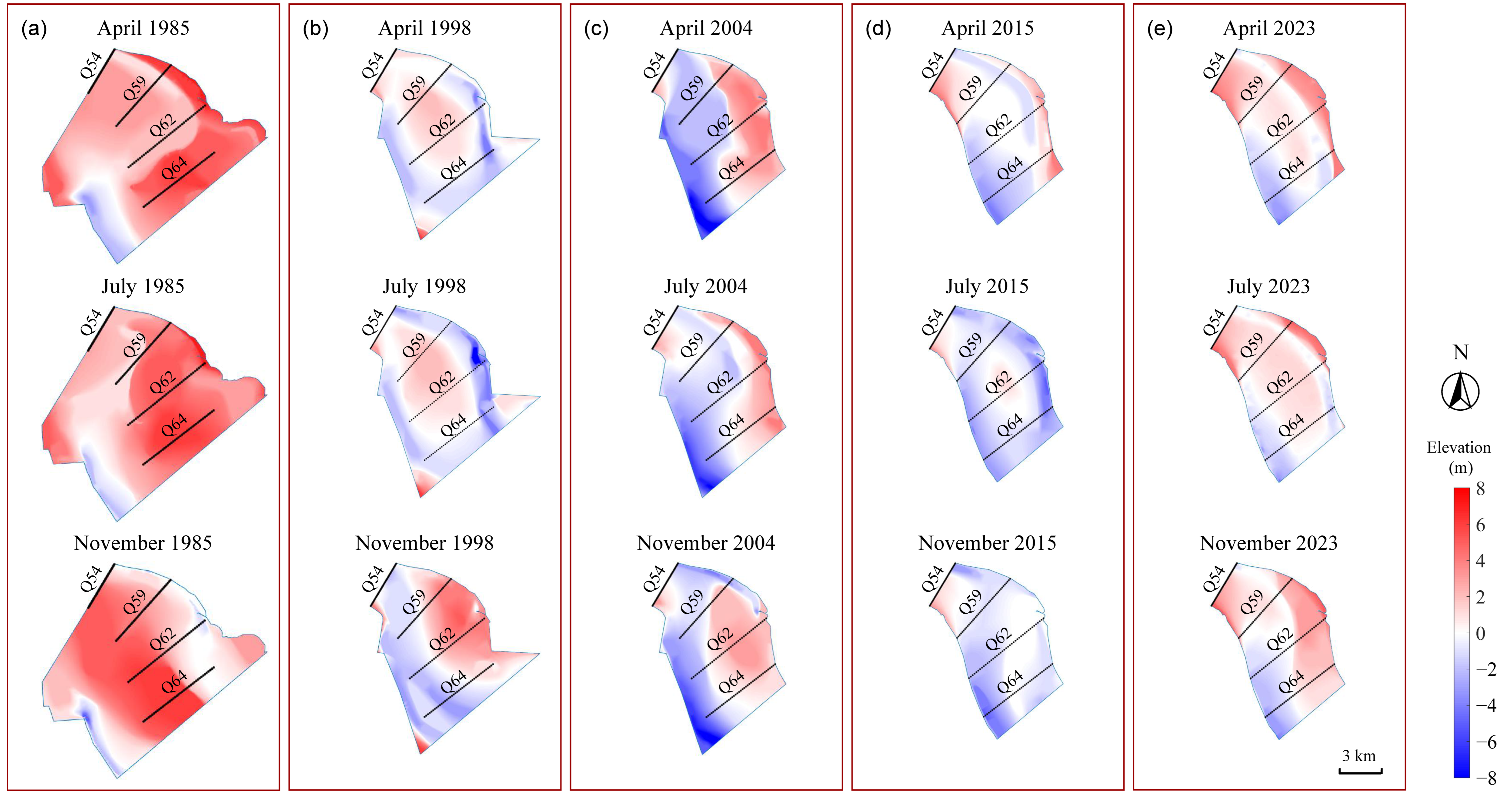
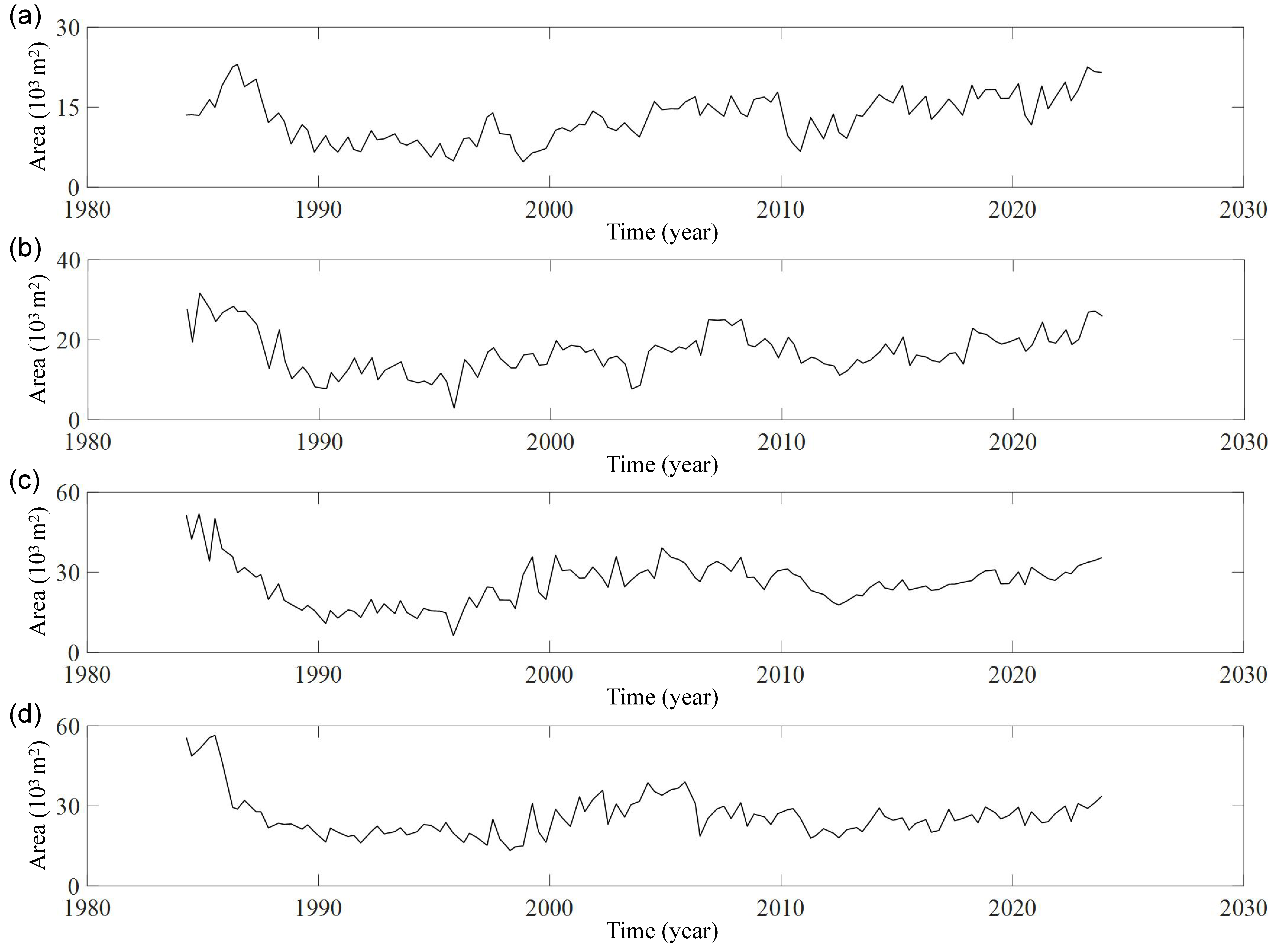
3.1. Morphodynamic Evolution

Figure 3 presents bathymetric charts depicting elevation changes in the study area for the years 1985, 1998, 2004, 2015, and 2023, with surveys conducted in April, July, and November. The years 1985 and 2004 were typical dry years, while 1998 and 2015 were typical wet years, and 2023 was a typical normal year. Wet, normal, and dry years correspond to runoff frequencies of 25%, 50%, and 75%, respectively. Due to intensive human activities, the reclaimed area in the study region increased by more than 46% from 1985 to 2023. The data exhibit consistent seasonal patterns, with higher elevations observed in April and November, and lower elevations in July. This trend is attributed to increased sediment erosion during the wet season due to higher runoff and river discharge, and sediment deposition during the dry seasons when hydrodynamic forces are less intense. Wet years (1998, 2015) are characterized by significant sediment movement, with pronounced erosion and deposition cycles, while normal years (2023) display less extreme but similar seasonal variations. During dry years, the main channel in the study area tends to be closer to the southern bank, whereas in wet years, the main channel exhibits significant oscillations between the south and north within the year. These charts underscore the dynamic nature of tidal flats.

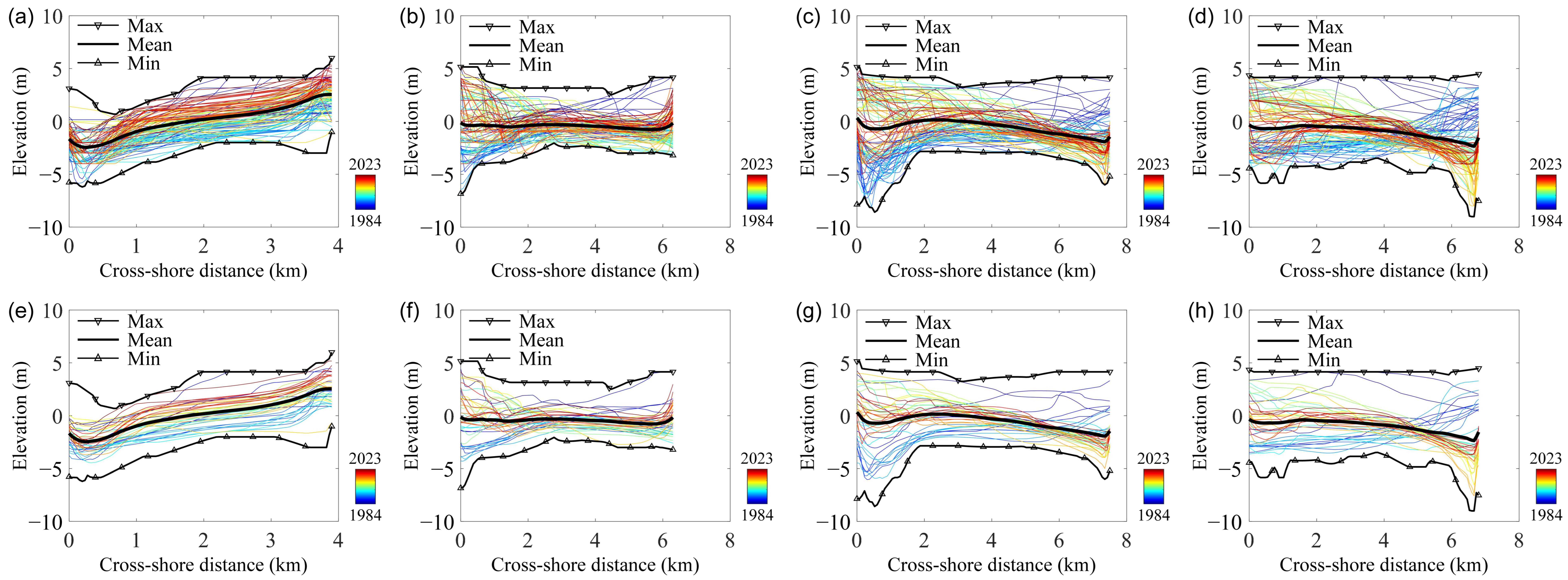
3.2. Tidal Flat Profiles

Figure 4 illustrates the topographic evolution of profiles Q54, Q59, Q62, and Q64 in the study area from 1984 to 2023, with measurements taken in April, July, and November, as well as annual average profiles. Profile Q54 displays a more confined range of elevations, indicating less variability and a more stable state. Conversely, profile Q59 shows significant elevation fluctuations, suggesting active erosion or deposition. Profiles Q62 and Q64 experience subtle elevation changes from 0 to 3 km before stabilizing, potentially reflecting phases of sediment accumulation or erosion followed by steadier conditions. The data reveal significant seasonal variations, with higher elevations generally observed in April and November and lower elevations in July. The annual average profile plots do not show a clear monotonic increasing or decreasing trend over time. However, the annual average elevations of the tidal flats in recent years tend to approximate the mean values observed over the entire period. The differences in these profiles may underscore the interactions of geomorphological processes shaped by both natural forces and human activities.

Figure 5 illustrates the temporal changes in the cross-sectional area above the historical minimum elevation for four coastal profiles (Q54, Q59, Q62, and Q64) from 1984 to 2023. Each profile demonstrates unique variations in geomorphological behavior over the study period. Profile Q54 shows a stable trend with minor fluctuations, indicating a gradual sediment accumulation or reduced erosion. In contrast, Profile Q59 initially displays a significant decrease in area, suggesting enhanced erosional activity or subsidence before stabilizing after 1996, potentially due to sediment deposition. Profile Q62 reveals a general decline until 1996, followed by increased variability, which may reflect alternating erosion and deposition influenced by changing hydrodynamic conditions or anthropogenic factors. Profile Q64 exhibits a sharp decline in area early in the record, stabilizing at a lower level from 1990 onwards with fewer fluctuations, possibly reflecting severe erosional events or practical mitigation efforts. These variations highlight the complex interactions between environmental forces and geomorphic responses.

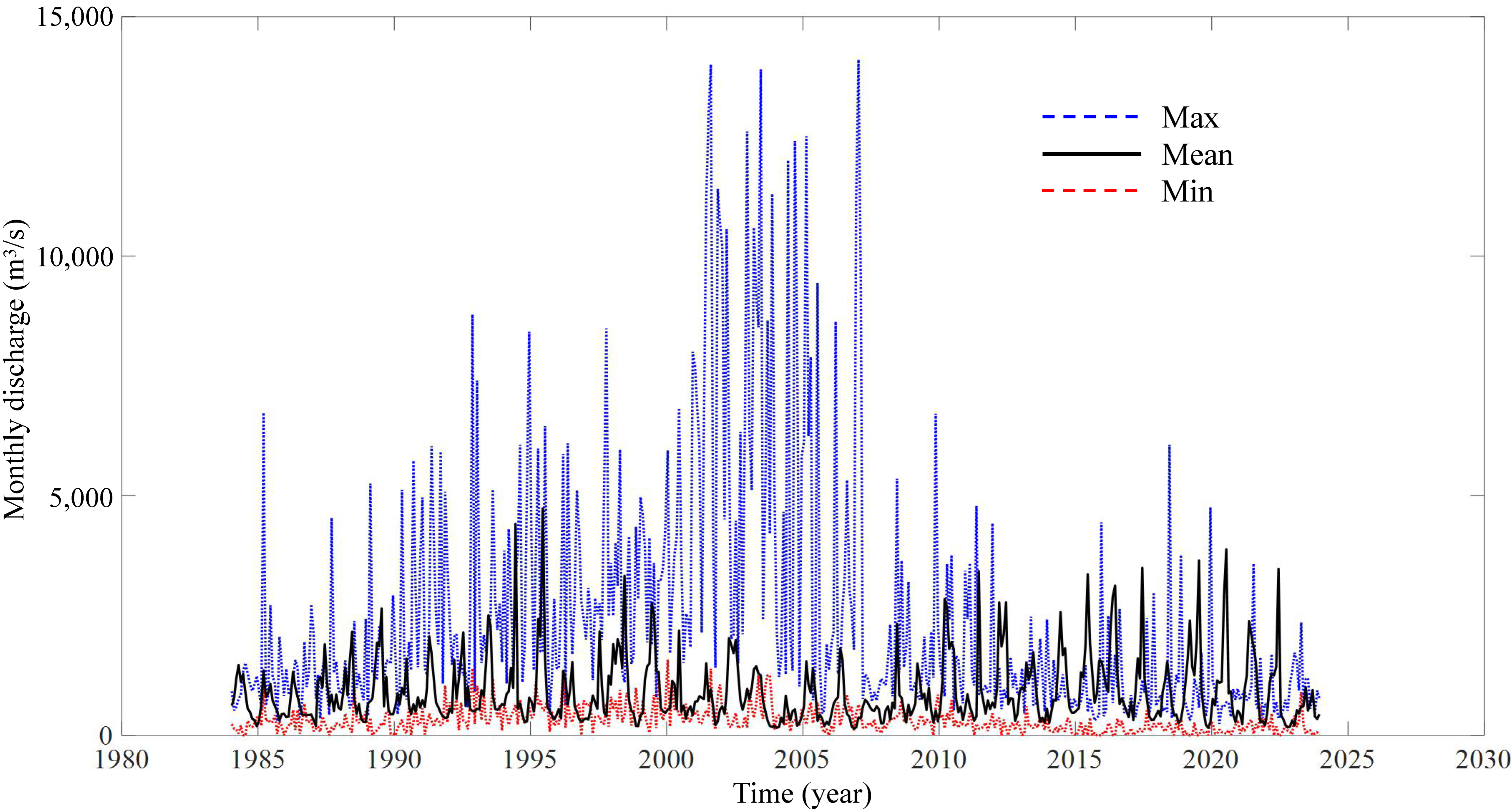
3.3. Hydrodynamic Conditions

Figure 6 presents a detailed time series analysis of the maximum, mean, and minimum monthly average runoff at the Fuchun River Hydropower Station from 1984 to 2023. The data reveal significant seasonal and interannual fluctuations, particularly in the maximum runoff (blue dashed line), likely due to seasonal floods caused by intense rainfall. Meanwhile, the mean runoff (black solid line) shows less pronounced changes, suggesting a relatively steady average hydrological contribution over the years despite monthly extremes. The minimum runoff (red dashed line) displays the most minor variability, reflecting stable base flow levels less affected by short-term weather changes. This analysis emphasizes the significant seasonal influence on river discharge, driven by regional weather patterns like plum rains or typhoons.

Figure 7 displays the monthly average tide ranges at the Yanguan and Ganpu Hydrological Stations from 1984 to 2023, showing the temporal changes in tidal behavior that are essential for topographic evolution. Over the past 40 years, the tidal range at Ganpu has shown minimal change compared to Yanguan, with only a slight increasing trend, largely due to the impact of reclamation [56]. On the other hand, the tide ranges at Yanguan show much more variability, with distinct peaks and troughs indicating dynamic environmental conditions and potentially higher sediment transport rates. Changes in river discharge, shifts in estuary bathymetry, or human activities such as reclamation altering the bottom friction at the riverbed may influence this variability at Yanguan. By comparing these two sites, we can see the significant impact of localized environmental and human factors on tidal consistency, affecting sediment transport dynamics and coastal morphology.

3.4. Empirical Orthonormal Functions and Principal Components

EOF analysis was employed to decompose the elevation data of four profiles from 1984 to 2023, identifying the principal modes of long-term evolution of tidal flats from both temporal and spatial viewpoints, and analyzing their characteristics over time. Figure 8 displays the proportional contribution of the first five eigenvectors (Eof1 to Eof5) across the four profiles (Q54, Q59, Q62, and Q64), providing a detailed depiction of the dominant patterns and variability within the spatial data throughout the study period. Eof1 is the most significant eigenvector, explaining between 50% and 63% of the total variability; this suggests a strong underlying mode of variability across different spatial locations. Eof2 consistently contributes between 31% and 39% to the total variability; this indicates a secondary but still substantial mode of variation. The contributions of Eof3 to Eof5 are relatively minor, collectively accounting for less than 10% of the variability in each profile; this implies that higher-order modes have less influence on the overall variability. This distribution demonstrates that while a few key patterns, primarily through Eof1 to Eof3, capture the majority of spatial variability, the additional spatial orthonormal functions offer vital insights into more complex spatial dynamics and localized phenomena. The first three eigenfunctions collectively account for over 90% of the total variance, underscoring the primary evolutionary characteristics of the tidal flats.

Figure 9 presents the spatial variability captured by the first three spatial eigenfunctions (Eof1 to Eof3) for coastal profiles Q54, Q59, Q62, and Q64. Across all profiles, Eof1 demonstrates a consistent underlying trend of elevation change; this suggests that Eof1 captures the dominant mode of spatial variability, reflecting the overall topographic gradient. For example, in Profile Q54, it depicts a central elevation feature, similar to the arithmetic mean profile of the data (Figure 4a), and in Q64, it shows a consistent elevation increase across the profile. Eof2 shows moderate fluctuations, indicating secondary modes of variability, while Eof3 exhibits more pronounced fluctuations, capturing finer-scale variability and localized features within the profiles. These fluctuations may be associated with smaller-scale morphological features or intermediate processes influencing sediment distribution. In Profile Q59, Eof2 notably peaks in the mid-section, suggesting features such as a dune or sediment bar, while in Profiles Q62 and Q64, these spatial eigenfunctions highlight subtle but overlapping geomorphological influences that suggest complex sediment dynamics. Eof1 captures the primary trend, while Eof2 and Eof3 reveal secondary and tertiary modes of variability. The distinct patterns displayed by the eigenfunctions across the profiles highlight the diverse geomorphological processes occurring, ranging from gradual sediment deposition to distinct elevation changes.

Figure 10 displays the first three principal components (cEof1, cEof2, and cEof3) for profiles Q54, Q59, Q62, and Q64 from 1980 to 2023, offering insights into the evolution of coastal processes shaped by hydrodynamic forces and human activities over the 40-year observation period. Across all profiles, cEof1 demonstrates significant fluctuations, indicating substantial variability in the primary mode, with a trend towards stabilization in recent years. cEof2 shows consistent moderate fluctuations, reflecting stable secondary modes influenced by periodic patterns. In addition, cEof3 exhibits minor fluctuations, indicating stability in the tertiary mode. While all profiles show similar overall patterns, the amplitude and timing of peaks and troughs in cEof1 vary, suggesting that specific events influencing each profile differ. For instance, Q59 and Q64 display more pronounced peaks in the mid-1990s compared to other profiles. The consistent pattern of variability across profiles highlights the influence of both natural and anthropogenic factors on the tidal flats, with cEof1 capturing the dominant mode of variability, cEof2 reflecting intermediate processes, and cEof3 representing finer-scale or localized changes. This analysis underscores the importance of understanding these principal components to decipher the temporal dynamics of tidal flats and inform effective coastal management strategies. Frequent changes in tidal flat elevations present significant challenges for coastal management. Coastal managers should implement regular monitoring and data collection, allowing for flexible and iterative decision-making based on the latest data.

Using Equation (2), the profile morphology can be reconstructed from the EOF analysis results. Figure 11 illustrates the reconstruction of coastal profiles for Q54, Q59, Q62, and Q64 in July 1989 and July 2010, using the first three eigenfunctions. It indicates that the first three eigenfunctions effectively capture the elevation changes across different years and locations. While profiles Q54, Q62, and Q64 exhibit a strong match between observed and reconstructed profiles, profile Q59 in July 1985 shows some deviations, particularly around the 2.8 km mark. This suggests that additional eigenfunctions may be needed to capture finer details or account for local variations. The consistency of accurate reconstruction from 1985 to 2015 suggests stability in the dominant modes of variability over this period, indicating that the primary processes affecting tidal flat morphology have remained largely unchanged. The effective reconstruction across different profiles highlights the spatial consistency in geomorphological processes, influenced by hydrodynamic conditions and sediment transport. However, the observed deviations, especially in profile Q59, suggest that finer details and local variations are not fully captured by the first three eigenfunctions. This indicates the need for high-quality data and a more detailed analysis, integrating EOF analysis with additional methods.

3.5. Mutation Analysis of the Principal Components

Figure 12, Figure 13 and Figure 14 illustrate the use of statistical tests to identify change-points in the first three principal components, labeled as cEof1 in Figure 12, cEof2 in Figure 13, and cEof3 in Figure 14. Each figure, from panels (a–d), presents results from the Mann–Kendall test for profiles Q54, Q59, Q62, and Q64, respectively. The test statistics (UF for upward trends and UB for downward trends) are graphed over time. A dashed line at the 0.05 significance level marks the threshold for rejecting the null hypothesis of no trend. Notably, the intersection of the UF and UB lines indicates potential change-points, suggesting shifts in the trend. Panels (e–h) in each figure apply a Moving T-test technique to assess the stationarity of the principal components at these profiles. This test measures mean changes across a moving window (specified here as n₁ = n₂ = 15) and is useful for pinpointing periods where the component means notably deviate from zero, indicating non-stationary behavior. By employing both the Mann–Kendall and Moving T-tests, this dual-method approach identifies and confirms change-points in the data. It effectively highlights shifts in both the central tendency and variability of the principal components, thereby enhancing the reliability of the findings.

Figure 12a illustrates that for profile Q54, the principal component cEof1 started showing an upward trend around 2012, which intensified notably after 2016, surpassing the critical significance level of 0.05. The UF and UB curves intersect within the critical interval. Analysis of this intersection position and the Moving T-test results (Figure 12e) suggests that the principal component cEof1 for profile Q54 experienced a sudden change around 2013. Similarly, in profiles Q59 (Figure 12b,f) and Q62 (Figure 12c,g), the principal component cEof1 underwent significant shifts around 2011 and 1999, respectively. However, no such change was observed in the principal component cEof1 of profile Q64 (Figure 12d,h). These shifts in cEof1 may be associated with alterations in hydrodynamic processes, as depicted in Figure 7. Notably, the monthly average tidal range at Yanguan demonstrated a significant decreasing trend around 1999 and 2011.

Figure 13b illustrates that the principal component cEof2 for profile Q59 initially showed an upward trend during the 1980s, but started to decline in the 1990s with a notable reduction beginning in 1994, which significantly surpassed the critical significance level of 0.05. The UF and UB curves meet within a critical range. The point of this convergence and the outcomes from the Moving T-test (Figure 13f) suggest that around 1988, there was a marked shift in the principal component cEof2 associated with profile Q59. In a similar vein, the principal component cEof2 for profiles Q62 (Figure 13c,g) and Q64 (Figure 13d,h) also experienced significant changes around 1987 and 1997, respectively. In contrast, no alterations were detected in the principal component cEof2 for profile Q54 (Figure 13a,e). These variations in cEof2 could be linked to human activities, as depicted in Figure 2a, particularly noting the major land reclamation efforts on the north bank of the Jianshan Bend beginning in 1998 and on the south bank starting in 1986.

Figure 14a shows that the principal component cEof3 for profile Q54 exhibited a variable pattern before 2010, but a significant decline began post-2010, becoming markedly notable after 2015 and well beyond the critical significance threshold of 0.05. The UF and UB curves cross within the critical range. The analysis of where these curves intersect and the results from the Moving T-test (Figure 14e) reveal that around 2011, the principal component cEof3 for profile Q54 underwent a major change. Similarly, the year of change for profile Q59 was identified around 2010 (Figure 14b,f), though no significant changes were detected in the principal component cEof3 for profiles Q62 (Figure 14c,g) and Q64 (Figure 14d,h). Like cEof1, the alteration in cEof3 is also linked to hydrodynamic processes.

3.6. Spectrum Analysis of the Principal Components

Figure 15 provides a detailed spectral analysis of the first three principal components (cEof1, cEof2, and cEof3) in relation to the monthly mean tidal range series at Yanguan, focusing on cross-spectrum, coherence, and phase spectra for profiles Q54, Q59, Q62, and Q64. The cross-spectral analysis examines the correlation between two time series in the frequency domain, and the cross-spectrum plots demonstrate how signal power varies across different periods, reflecting varied spectral components influenced by tidal ranges. The coherence plots show the correlation level across frequencies, with changes in coherence indicating an uneven influence of tidal ranges on the principal components, possibly due to local geomorphological factors. The phase spectrum displays differences in phase angles, highlighting specific timing alignments between the signals and tidal cycles. Coherence, a real value ranging from 0 to 1, where 0 represents no correlation and 1 indicates maximum correlation at a specific frequency, plays a crucial role in determining significant coherence levels necessary for calculating phase shifts between two series [55].

The impact of the monthly mean tidal range series on the principal components is clearly visible through diverse patterns in cross-spectrum power, coherence, and phase angles. These variations suggest that the principal components capture different modes of variation influenced by tidal cycles, ranging from periodic oscillations to event-driven responses. The coherence differences across profiles indicate that while some principal components closely match tidal patterns, others are influenced by additional factors. Figure 15 offers insights into the frequency domain of these principal components, highlighting intricate connections between the principal components and tidal patterns, with wider implications for coastal processes and geomorphological changes. Specifically, in profiles Q54 and Q64, cEof1 shows a strong correlation with tidal level variations at Yanguan in the low-frequency range, with periods longer than 7.7 years. Conversely, in profiles Q59 and Q62, cEof1 correlates with changes in the monthly mean tidal range on a roughly annual basis. Meanwhile, cEof2 correlates strongly with the mean tidal range over periods longer than one year, and cEof3 shows a high correlation with tidal range over periods shorter than 1.5 years.

Table 1. Results of spectral analysis of the first three principal components (cEof1, cEof2, and cEof3) in relation to the monthly mean tidal range series at Yanguan (Tr1) and Ganpu (Tr2), as well as the monthly mean discharge at the Fuchun River Hydropower Station (Q). The table includes the period (in year), the coherence coefficient, and the phase shift (in month) corresponding to the maximum coherence coefficient.

Profile	Factor	Tr1 and Principal Components			Tr2 and Principal Components			Q and Principal Components
		cEof1	cEof2	cEof3	cEof1	cEof2	cEof3	cEof1	cEof2	cEof3
Q54	Period (year)	>7.76	1.00	1.42	>7.76	0.97	2.44	>7.76	0.99	1.39
	Coherence coefficient	>0.78	0.68	0.56	>0.84	0.54	0.47	>0.78	0.79	0.52
	Phase shift (month)	Null	−4	−1	Null	−5	−13	Null	4	−6
Q59	Period (year)	0.99	4.06	0.96	0.98	0.97	4.06	0.99	0.98	4.27
	Coherence	0.57	0.65	0.41	0.81	0.60	0.49	0.83	0.62	0.61
	Phase shift (month)	−3	−21	2	−5	2	−18	5	0	1
Q62	Period (year)	1.00	>7.76	0.98	0.97	>7.76	0.99	1.00	>7.76	1.05
	Coherence	0.53	>0.80	0.45	0.55	>0.68	0.46	0.67	>0.71	0.65
	Phase shift (month)	4	Null	−3	2	Null	−4	0	Null	6
Q64	Period (year)	>7.76	1.98	0.97	>7.76	0.73	0.97	>7.76	1.33	0.99
	Coherence	>0.54	0.46	0.42	>0.45	0.48	0.53	>0.53	0.49	0.69
	Phase shift (month)	Null	−8	−3	Null	−2	−4	Null	−1	5

shows a comprehensive spectral analysis of the first three principal components (cEof1, cEof2, and cEof3) in relation to critical hydrological parameters. These parameters include the monthly mean tidal ranges at Yanguan (Tr1) and Ganpu (Tr2), as well as the monthly mean discharge at the Fuchun River Hydropower Station (Q). The table details the periodicity and phase shift associated with the maximum coherence coefficients, providing insights into the frequency and phase relationships between the principal components and these hydrological measures. The coherence coefficients, which indicate the strength of these relationships, show varying degrees of correlation, highlighting the distinct temporal dynamics at each location. The analysis shows that cEof1 consistently exhibits long-term periodicities and high coherence coefficients, indicating it captures the primary mode of variability associated with long-term hydrological changes. Conversely, cEof2 and cEof3 capture shorter-term variations, reflecting more transient factors. The phase shifts provide insights into the temporal alignment between the principal components and the hydrological data, with varying degrees of lead or lag.

The variations in the spectral analysis outcomes among the principal components emphasize the differing dynamics of the coastal environment. Each eigenfunction seems to capture unique modes of variability, shaped by elements like freshwater discharge, tidal mixing, and dynamics of coastal sediments. The range in periodicity and phase shifts highlights the complicated interactions between hydrological and geomorphological factors, along with possible external influences such as climate variation or human impacts.

4. Discussion

4.1. Dominant Modes of Variability

This study highlights the value of EOF analysis in identifying the dominant variability modes within tidal flat profiles along the curved coast of the QRE. It reveals specific variability modes closely associated with key geomorphological and hydrodynamic processes. Eof1 consistently accounts for the greatest variance, emphasizing its role as the main mode of spatial variability, likely representing dominant geomorphological activities such as sediment accumulation or erosion, and reflecting the overall topographic gradient. Eof2, while contributing less to the variance, captures significant secondary geomorphological characteristics related to localized sediment dynamics, showing moderate fluctuations indicative of secondary variability. Eof3, along with higher-order modes, contributes even less to the variability, but its pronounced fluctuations are essential for understanding finer-scale variability and localized features. This pattern, in which the initial few modes dominate the variability, is corroborated by other coastal geomorphological studies, thereby reinforcing the credibility of these findings [24,47].

Meanwhile, this study confirms that EOF analysis effectively separates the complex factors shaping the evolution of tidal flat profiles. It shows that both the temporal and spatial components of the data can be analyzed independently, allowing us to pinpoint specific riverbank processes accurately. When analyzing the first four empirical orthogonal function modes from the dataset (Figure 16), each mode reveals significant variations that explain the changes over time and space. For example, in profile Q54, the first mode suggests a rotating profile with a node near the northern bank, while the second mode indicates oscillations with consistent amplitudes except at the ends. In profile Q59, oscillations with larger amplitudes at the ends characterize the first mode, and the second mode points to rotation around a one-third node. Profile Q62 exhibits a comparable rotation in its initial two modes, which show slight symmetry. Profile Q64 resembles Q59, with its first mode displaying oscillations throughout the section and the second mode demonstrating central rotation. The third and fourth modes in all profiles show patterns of rotation that are significant only in certain years. The ability of EOF analysis to distinguish these different modes helps us understand critical processes like sediment exchange and erosion, essential for grasping the dynamics of tidal flat. This understanding is akin to what is observed in embayed beach rotation studies [57,58].

4.2. Conceptual Model of Morphodynamic Evolution

After collecting and organizing topographic, hydrological, and sediment data, we conducted EOF analyses to identify elevation changes, assess the impacts of river discharge and tidal variations, and determine sediment transport dynamics. These detailed analyses allowed us to mark elevation changes and sediment transport accurately. Field observations were conducted to verify these findings. Consequently, we developed a new conceptual model illustrating the physical processes driving morphodynamic evolution. This model can be used to examine the effects of unique geographic formations and tidal dynamics in curved coastal regions, such as the Jianshan Bend, on sediment transport and exchange patterns. Figure 17 presents the conceptual model of tidal flat variability at the Jianshan Bend during the flood season and the dry season. The changes in tidal flat profiles include rotation and oscillation, while the movement of sediment involves alongshore and cross-shore sediment exchanges.

During the flood season, increased river discharge and frequent precipitation intensify sediment movement, leading to observable alterations along the shoreline and in submerged areas. For example, Profile Q54 demonstrates significant lateral sediment shifts, resulting in a clockwise rotation of the profile. Conversely, Profile Q59 exhibits erosion attributed to longitudinal sediment transport along the shore. Profile Q62 is characterized by erosion in its raised sandy bar regions, which continue to expand even as they reduce in elevation. Profile Q64, on the other hand, displays consistent sediment patterns, indicating stable hydrological conditions across seasons.

In the dry season, sediment accretion intensifies across all observed profiles, demonstrating a clear seasonal pattern. In Profiles Q59 and Q64, sediment brought in by incoming tides builds up along the coast, enlarging the mudflats. However, the profile Q54 rotates in the counterclockwise direction, which is the opposite of the flood season. For Profile Q62, sediment builds up on the northern side while slightly eroding on the southern side, also suggesting a counterclockwise rotation. The sandy bars increase in height but decrease in overall size. The function of these coastal bars as temporary storage for eroded sediment from mudflats is vital [35]. This observation underlines the importance of accounting for both the physical geography and seasonal changes in managing coastal areas. These findings support previous studies indicating that curved coastlines, which differ significantly from straight ones, introduce unique movements of water and sediment due to their shape [10,11].

The results of this research are essential for coastal management and protection. By identifying key patterns of variability, the study clarifies the geomorphological processes and hydrodynamic conditions that influence the development of tidal flats. This knowledge is crucial for developing predictive strategies and managing these important coastal regions effectively. Specifically, discerning distinct patterns of variability assists coastal managers in focusing their monitoring and intervention efforts on areas prone to significant or sudden changes.

4.3. Addressing Limitations and Suggestions for Future Research

Although EOF analysis effectively identifies dominant variability modes, this study encountered significant limitations due to the lack of continuous, high-quality datasets over long durations. The four profiles are clearly insufficient in providing comprehensive spatial resolution, and their accuracy is limited. Additionally, the temporal resolution of data acquisition, with measurements conducted only three times a year, is inadequate for capturing necessary variations and trends. To improve data acquisition, we recommend increasing the number of profiles, enhancing their spatial resolution and accuracy, and conducting measurements more frequently throughout the year. This issue highlights the need for improved data collection techniques and the integration of advanced statistical methods to enhance the analysis. Liu et al. [47] emphasize the importance of comprehensive data to detect subtle changes in tidal flats influenced by various factors such as sediment supply, hydrodynamic processes, human activities, and climate change. The lack of high-resolution datasets hinders the ability to effectively monitor and predict subtle or gradual changes in tidal flats.

To tackle these challenges, it is essential for future research to prioritize obtaining higher-resolution data and utilizing advanced analytical techniques. By integrating EOF analysis with methods such as wavelet analysis or canonical correlation analysis, it is possible to strengthen the reliability of findings and provide deeper insights into the temporal and spatial dynamics of tidal flats [35]. For example, wavelet analysis is adept at capturing localized variations in time and frequency, essential for detecting short-term or episodic events. On the other hand, canonical correlation analysis is valuable for identifying relationships between multiple variable sets, thus aiding in the comprehension of interactions between tidal flat profiles and external influences like hydrodynamic conditions or human activities.

5. Conclusions

This study employed EOF analysis to explore the long-term evolution of tidal flats at the Jianshan Bend in the QRE. The research decomposed elevation data from four profiles to identify primary modes of spatial and temporal variability. Data were collected from bathymetric surveys conducted three times annually from 1984 to 2023, aiming to uncover the main geomorphological and hydrodynamic processes affecting the tidal flats. The methodology involved a comprehensive EOF analysis, which effectively isolated the complex factors driving the evolution of these tidal flat profiles.

The results revealed that the first mode accounted for the majority of the variance, reflecting dominant geomorphological activities such as sediment accumulation or erosion. Higher-order modes captured finer-scale variability and localized features. The efficacy of EOF analysis in identifying specific riverbank processes and understanding the dynamics of tidal flat evolution was demonstrated. The study showed patterns of sediment movement and elevation changes between flood and dry seasons, emphasizing the seasonal effects on tidal flat morphology. The conceptual model developed from these findings offers a framework for predicting future changes and guiding coastal management strategies.

However, the study encountered limitations due to the insufficient spatial and temporal resolution of the data. The four profiles were inadequate for providing comprehensive spatial coverage, and the data collection frequency of three times a year failed to capture all necessary variations. Future research should aim to increase the number of profiles, enhance spatial and temporal resolution, and integrate advanced analytical techniques such as wavelet and canonical correlation analysis to improve the reliability of findings and deepen the understanding of tidal flat dynamics.

References

1. Chen, Z.L.; Lee, S.Y. Tidal flats as a significant carbon reservoir in global coastal ecosystems. Front. Mar. Sci. 2022, 9, 900896. [Google Scholar] [CrossRef]
2. Shimizu, T.; Senzaki, M.; Fujioka, Y.; Seino, S. Relative importance of tidal flats and artificial habitats for two spoonbill species and related interspecific differences. Avian Res. 2023, 14, 100107. [Google Scholar] [CrossRef]
3. Reed, D.; Van Wesenbeeck, B.; Herman, P.M.J.; Meselhe, E. Tidal flat-wetland systems as flood defenses: Understanding biogeomorphic controls. Estuar. Coast. Shelf Sci. 2018, 213, 269–282. [Google Scholar] [CrossRef]
4. Fortune, J.; Butler, E.C.V.; Gibb, K. Estuarine benthic habitats provide an important ecosystem service regulating the nitrogen cycle. Mar. Environ. Res. 2023, 190, 106121. [Google Scholar] [CrossRef] [PubMed]
5. Brown, D.R.; Marotta, H.; Peixoto, R.B.; Enrich-Prast, A.; Barroso, G.C.; Soares, M.L.G.; Machado, W.; Perez, A.; Smoak, J.M.; Sanders, L.M.; et al. Hypersaline tidal flats as important “blue carbon” systems: A case study from three ecosystems. Biogeosciences 2021, 18, 2527–2538. [Google Scholar] [CrossRef]
6. Zhang, W.; Ouyang, K.; Zhang, X.; Wang, A.; Yu, Q.; Ye, X.; Yao, C. Tidal flat erosion processes and their dynamic mechanisms on the south side of Sheyang River estuary, Jiangsu Province. J. Mar. Sci. Eng. 2024, 12, 687. [Google Scholar] [CrossRef]
7. Zhou, Z.; Liang, M.; Chen, L.; Xu, M.; Chen, X.; Geng, L.; Li, H.; Serrano, D.; Zhang, H.; Gong, Z.; et al. Processes, feedbacks, and morphodynamic evolution of tidal flatemarsh systems: Progress and challenges. Water Sci. Eng. 2022, 15, 89–102. [Google Scholar] [CrossRef]
8. Wright, L.D.; Thom, B.G. Coastal morphodynamics and climate change: A review of recent advances. J. Mar. Sci. Eng. 2023, 11, 1997. [Google Scholar] [CrossRef]
9. Munoz-Perez, J.J.; Medina, R.; Tejedor, B. Evolution of longshore beach contour lines determined by EOF method. Sci. Mar. 2001, 65, 393–402. [Google Scholar] [CrossRef]
10. Gijsman, R.; Ruessink, B.G.; Visscher, J.; Schlurmann, T. Observations on decadal sandbar behaviour along a large-scale curved shoreline. Earth Surf. Process. Landforms 2021, 46, 490–503. [Google Scholar] [CrossRef]
11. Rutten, J.; Dubarbier, B.; Price, T.D.; Ruessink, B.G.; Castelle, B. Alongshore variability in crescentic sandbar patterns at a strongly curved coast. J. Geophys. Res. Earth Surf. 2019, 124, 2877–2898. [Google Scholar] [CrossRef]
12. Rutten, J.; Ruessink, B.G.; Price, T.D. Observations on sandbar behaviour along a man-made curved coast. Earth Surf. Process. Landforms 2018, 43, 134–149. [Google Scholar] [CrossRef]
13. Li, Y.; Pan, D.Z.; Chanson, H.; Pan, C.H. Real-time characteristics of tidal bore propagation in the Qiantang River Estuary, China, recorded by marine radar. Cont. Shelf Res. 2019, 180, 48–58. [Google Scholar] [CrossRef]
14. Li, Y.; Pan, D.Z.; Cheng, W.L.; Pan, C.H. Tidal stream energy resource assessment in the Qiantang River Estuary, China. Int. J. Sustain. Energy 2018, 37, 704–717. [Google Scholar] [CrossRef]
15. Bearman, J.A.; Friedrichs, C.T.; Jaffe, B.E.; Foxgrover, A.C. Spatial trends in tidal flat shape and associated environmental parameters in South San Francisco Bay. J. Coast. Res. 2010, 26, 342–349. [Google Scholar] [CrossRef]
16. Hu, Y.; Cao, M.; Ma, A.; Dou, X.; Wen, Y. An analysis of the periodic evolution of the Jingjiang sandbank in the tidal reach of the Yangtze River. Water 2020, 12, 1652. [Google Scholar] [CrossRef]
17. Alvarez, F.; Pan, S. Predicting coastal morphological changes with empirical orthogonal function method. Water Sci. Eng. 2016, 9, 14–20. [Google Scholar] [CrossRef]
18. Hannachi, A.; Jolliffe, I.T.; Stephenson, D.B. Empirical orthogonal functions and related techniques in atmospheric science: A review. Int. J. Climatol. 2007, 27, 1119–1152. [Google Scholar] [CrossRef]
19. Neha; Pasari, S. A review of empirical orthogonal function (EOF) with an emphasis on the co-seismic crustal deformation analysis. Nat. Hazards 2022, 110, 29–56. [Google Scholar] [CrossRef]
20. Vincent, L.; Dolan, R.; Hayden, B.; Resio, D. Systematic variations in barrier-island topography. J. Geol. 1976, 84, 583–5594. [Google Scholar] [CrossRef]
21. Resio, D.T.; Dolan, R.; Hayden, B.P.; Vincent, C.L. Systematic variations in offshore bathymetry. J. Geol. 1977, 85, 105–113. [Google Scholar] [CrossRef]
22. Dolan, R.; Hayden, B.P.; Felder, W. Systematic variations in inshore bathymetry. J. Geol. 1977, 85, 129–141. [Google Scholar] [CrossRef]
23. Winant, C.D.; Inman, D.L.; Nordstrom, C.E. Description of seasonal beach changes using empirical eigenfunctions. J. Geophys. Res. 1975, 80, 1979–1986. [Google Scholar] [CrossRef]
24. Aubrey, D.G. Seasonal patterns of onshore/offshore sediment movement. J. Geophys. Res. 1979, 84, 6347–6354. [Google Scholar] [CrossRef]
25. Aubrey, D.G. The statistical prediction of beach changes in Southern California. J. Geophys. Res. 1980, 85, 3264–3276. [Google Scholar] [CrossRef]
26. Clarke, D.J.; Eliot, I.G. Description of littoral, alongshore sediment movement from empirical eigen-function analysis. J. Geol. Soc. Aust. 1982, 29, 327–341. [Google Scholar] [CrossRef]
27. Rooynski, G. Data-driven modeling of multiple longshore bars and their interactions. Coast. Eng. 2003, 48, 151–170. [Google Scholar] [CrossRef]
28. Dai, Z.J.; Liu, J.T.; Lei, Y.P.; Zhang, X.L. Patterns of sediment transport pathways on a headland bay beach—Nanwan Beach, South China: A case study. J. Coast. Res. 2010, 26, 1096–1103. [Google Scholar] [CrossRef]
29. Miller, J.K.; Dean, R.G. Shoreline variability via empirical orthogonal function analysis: Part I temporal and spatial characteristics. Coast. Eng. 2007, 54, 111–131. [Google Scholar] [CrossRef]
30. Miller, J.K.; Dean, R.G. Shoreline variability via empirical orthogonal function analysis: Part II relationship to nearshore conditions. Coast. Eng. 2007, 54, 133–150. [Google Scholar] [CrossRef]
31. He, Y.; Wu, Y.; Lu, L.; Wu, M.; Chen, Y.; Yang, Y. Morphological change of the mouth bar in relation to natural and anthropogenic interferences. Cont. Shelf Res. 2019, 175, 42–52. [Google Scholar] [CrossRef]
32. Zhang, R.; Chen, L.; Liu, S.; Zhang, H.; Gong, W.; Lin, G. Shoreline evolution in an embayed beach adjacent to tidal inlet: The impact of anthropogenic activities. Geomorphology 2019, 346, 106856. [Google Scholar] [CrossRef]
33. Luo, J.; Dai, Z.; Wang, J.; Lou, Y.; Zhou, X.; Tang, R. Effects of human-induced riverine sediment transfer on deposition–erosion in the South Passage of the Changjiang (Yangtze) delta. J. Hydrol. 2023, 622, 129714. [Google Scholar] [CrossRef]
34. Kroon, A.; Larson, M.; Moller, I.; Yokoki, H.; Rozynski, G.; Cox, J.; Larroude, P. Statistical analysis of coastal morphological data sets over seasonal to decadal time scales. Coast. Eng. 2008, 55, 581–600. [Google Scholar] [CrossRef]
35. Short, A.D.; Trembanis, A.C. Decadal scale patterns in beach oscillation and rotation Narrabeen Beach, Australia—Time series, PCA and wavelet analysis. J. Coast. Res. 2004, 20, 523–532. [Google Scholar] [CrossRef]
36. Karunarathna, H.; Horrillo-Caraballo, J.M.; Ranasinghe, R.; Short, A.D.; Reeve, D.E. An analysis of the cross-shore beach morphodynamics of a sandy and a composite gravel beach. Mar. Geol. 2012, 299–302, 33–42. [Google Scholar] [CrossRef]
37. Kuriyama, Y.; Yanagishima, S. Investigation of medium-term barred beach behavior using 28-year beach profile data and Rotated Empirical Orthogonal Function analysis. Geomorphology 2016, 261, 236–243. [Google Scholar] [CrossRef]
38. Munoz-Perez, J.J.; Medina, R. Comparison of long-, medium- and short-term variations of beach profiles with and without submerged geological control. Coast. Eng. 2010, 57, 241–251. [Google Scholar] [CrossRef]
39. Wijnberg, K.M.; Terwindt, J.H.J. Extracting decadal morphological behaviour from high-resolution, long-term bathymetric surveys along the Holland coast using eigenfunction analysis. Mar. Geol. 1995, 126, 301–330. [Google Scholar] [CrossRef]
40. Lemke, L.; Miller, J.K. EOF analysis of shoreline and beach slope variability at a feeder beach constructed within a groin field at Long Branch, New Jersey. Coast. Eng. 2017, 121, 14–25. [Google Scholar] [CrossRef]
41. Dissanayake, N.G.; Frid, C.L.J.; Drylie, T.P.; Caswell, B.A. Ecological functioning of mudflats: Global analysis reveals both regional differences and widespread conservation of functioning. Mar. Ecol. Prog. Ser. 2018, 604, 1–20. [Google Scholar] [CrossRef]
42. Shi, B.; Wang, Y.P.; Du, X.; Cooper, J.R.; Li, P.; Li, M.L.; Yang, Y. Field and theoretical investigation of sediment mass fluxes on an accretional coastal mudflat. J. Hydro-Environ. Res. 2016, 11, 75–90. [Google Scholar] [CrossRef]
43. Zhang, K.; Jin, Q.; Wang, B. Seasonal Changes of the tidal flat from Jinhuigang to Caojing along the north bank of Hangzhou Bay. Chin. J. Oceannol. Limnol. 1993, 11, 321–332. [Google Scholar]
44. Li, H.; Yang, G. A study on equilibrium coastal profile s of the close tidal flat: A case study of Fengxian tidal flat. Chin. Geogr. Sci. 2002, 12, 55–60. [Google Scholar] [CrossRef]
45. Dai, Z.; Liu, J.T.; Fu, G.; Xie, H. A thirteen-year record of bathymetric changes in the North Passage, Changjiang (Yangtze) estuary. Geomorphology 2013, 187, 101–107. [Google Scholar] [CrossRef]
46. Dai, Z.; Liu, J.T.; Wen, W. Morphological evolution of the South Passage in the Changjiang (Yangtze River) estuary, China. Quat. Int. 2015, 380–381, 314–326. [Google Scholar] [CrossRef]
47. Liu, Y.; Xia, X.; Chen, S.; Jia, J.; Cai, T. Morphological evolution of Jinshan Trough in Hangzhou Bay (China) from 1960 to 2011. Estuar. Coast. Shelf Sci. 2017, 198, 367–377. [Google Scholar] [CrossRef]
48. Shimozono, T.; Tajima, Y.; Akamatsu, S.; Matsuba, Y.; Kawasaki, A. Large-scale channel migration in the Sittang River estuary. Sci. Rep. 2019, 9, 9862. [Google Scholar] [CrossRef]
49. Li, Y.; Pan, D. Tidal bore impact pressures on a trestle pier in the Qiantang River Estuary, China. Adv. Mech. Eng. 2022, 14, 1–12. [Google Scholar] [CrossRef]
50. Zeng, J.; Han, H.; Cheng, W. Experimental study on the plan line for river regulation for Jianshan Bend of Qiantang Estuary (in Chinese with English abstract). Donghai Mar. Sci. 2001, 19, 52–60. [Google Scholar]
51. Pan, C.; Han, Z. Research on Conservation and Regulation of the Qiantang River Estuary; China Water & Power Press: Beijing, China, 2017. (In Chinese) [Google Scholar]
52. Zhejiang Provincial Hydrology Bureau of China. Hydrological services. Available online: http://www.zjsw.cn/pages/channel.jsp?catId=1022 (accessed on 20 June 2024).
53. Kendall, M.G. Rank-Correlation Measures; Charles Griffin: London, UK, 1975. [Google Scholar]
54. Maidment, D.R. Handbook of Hydrology; McGraw-Hill: New York, NY, USA, 1993. [Google Scholar]
55. Trauth, M.H. MATLAB® Recipes for Earth Sciences, 3rd ed.; Springer: Berlin/Heidelberg, Germany, 2010. [Google Scholar]
56. Pan, C.; Zheng, J.; Cheng, G.; He, C.; Tang, Z. Spatial and temporal variations of tide characteristics in Hangzhou Bay and cause analysis (in Chinese with English abstract). Ocean Eng. 2019, 37, 1–11. [Google Scholar]
57. Loureiro, C.; Ferreira, O.; Cooper, J.A.G. Geologically constrained morphological variability and boundary effects on embayed beaches. Mar. Geol. 2012, 329–331, 1–15. [Google Scholar] [CrossRef]
58. Harley, M.D.; Turner, I.L.; Short, A.D. New insights into embayed beach rotation: The importance of wave exposure and cross-shore processes. J. Geophys. Res. Earth Surf. 2015, 120, 1470–1484. [Google Scholar] [CrossRef]
Figure 1. Location map of the Qiantang River Estuary and Jianshan Bend: (a) the Qiantang River Estuary in China; (b) observation profiles, created from Landsat imagery. Landsat imagery courtesy of the U.S. Geological Survey.
Jmse 12 01089 g001
Figure 2. Location of the study area: (a) reclamation process from the 1960s to the 2010s; (b) view of the Tashan Groin, illustrating how the tidal bore bypasses the Tashan Groin from east to west. Photo of the Tashan Groin is courtesy of Guohua Jin.
Jmse 12 01089 g002
Figure 3. Bathymetry charts of the study area in (a) 1985, (b) 1998, (c) 2004, (d) 2015, and (e) 2023. There were three surveys conducted each year in April, July, and November. The years 1985 and 2004 were typical dry years; 1998 and 2015 were typical wet years; and 2023 was a typical normal year. Wet, normal, or dry years correspond to runoff frequencies of 25%, 50%, and 75%, respectively.
Jmse 12 01089 g003
Figure 4. Topographic evolution of profiles (a) Q54, (b) Q59, (c) Q62, and (d) Q64 from 1984 to 2023 in April, July, and November; annual average profiles (e) Q54, (f) Q59, (g) Q62, and (h) Q64 from 1984 to 2023. The cross-shore distance was measured starting from the left bank, which corresponded to the north bank.
Jmse 12 01089 g004
Figure 5. Changes in the cross-sectional area above the historical minimum elevation for profiles (a) Q54, (b) Q59, (c) Q62, and (d) Q64, spanning the period from 1984 to 2023.
Jmse 12 01089 g005
Figure 6. Maximum, mean, and minimum monthly average runoff at the Fuchun River Hydropower Station, spanning the period from 1984 to 2023. The location of the Fuchun River Hydropower Station is marked in Figure 1.
Jmse 12 01089 g006
Figure 7. Monthly mean tidal range at the Yanguan and Ganpu Hydrological Stations, recorded over the period from 1984 to 2023. The positions of these two hydrological stations are marked in Figure 1.
Jmse 12 01089 g007
Figure 8. The proportional contribution of the first five eigenvectors across profiles Q54, Q59, Q62, and Q64.
Jmse 12 01089 g008
Figure 9. The first three spatial eigenfunctions (Eof1, Eof2 and Eof3) for profiles (a) Q54, (b) Q59, (c) Q62, and (d) Q64.
Jmse 12 01089 g009
Figure 10. The first three principal components (cEof1, cEof2 and cEof3) for profiles (a) Q54, (b) Q59, (c) Q62, and (d) Q64.
Jmse 12 01089 g010
Figure 11. Reconstruction of the profiles (a) Q54, (b) Q59, (c) Q62, and (d) Q64 in July 1985, and (e) Q54, (f) Q59, (g) Q62, and (h) Q64 in July 2015, using the first three eigenfunctions. Observed data were derived from direct measurements, while reconstructed data were calculated using Equation (2).
Jmse 12 01089 g011
Figure 12. Detection of change-points in the first principal component (cEof1). The Mann–Kendall test was applied to cEof1 at profiles (a) Q54, (b) Q59, (c) Q62, and (d) Q64. Additionally, a Moving T-test technique was used on cEof1 at profiles (e) Q54, (f) Q59, (g) Q62, and (h) Q64.
Jmse 12 01089 g012
Figure 13. Change-point detection in the second principal component (cEof2). Mann–Kendall test on cEof2 at profiles (a) Q54, (b) Q59, (c) Q62, and (d) Q64; Moving T-test technique applied to cEof2 at profiles (e) Q54, (f) Q59, (g) Q62, and (h) Q64.
Jmse 12 01089 g013
Figure 14. Change-point detection in the third principal component (cEof3). Mann–Kendall test on cEof3 at profiles (a) Q54, (b) Q59, (c) Q62, and (d) Q64; Moving T-test technique applied to cEof3 at profiles (e) Q54, (f) Q59, (g) Q62, and (h) Q64.
Jmse 12 01089 g014
Figure 15. Results of spectral analysis of the first three principal components (cEof1, cEof2 and cEof3) with the monthly mean tidal range series at Yanguan. Cross-spectrum of time series for profiles: (a) Q54, (b) Q59, (c) Q62, and (d) Q64. Coherence in the frequency domain for profiles: (e) Q54, (f) Q59, (g) Q62, and (h) Q64. Phase spectrum in radians for profiles: (i) Q54, (j) Q59, (k) Q62, and (l) Q64.
Jmse 12 01089 g015
Figure 16. Reconstruction of the first four empirical orthogonal function modes based on EOF analysis. Panels depict: (a) c1(t)e1(x), (b) c2(t)e2(x), (c) c3(t)e3(x), and (d) c4(t)e4(x). As defined in Equation (2), ck(t)ek(x) represents the reconstructed k-th mode of the original dataset.
Jmse 12 01089 g016
Figure 17. Conceptual model of tidal flat variability at the Jianshan Bend. (a) During the flood season and (b) during the dry season. The thin blue arrows represent the amplitude and direction of changes in section elevation, while the wide red arrows depict sediment transport dynamics, including alongshore and cross-shore sediment exchanges.
Jmse 12 01089 g017