
Optimization of Submerged Breakwaters for Maximum Power of a Point-Absorber Wave Energy Converter Using Bragg Resonance


Abstract
:1. Introduction
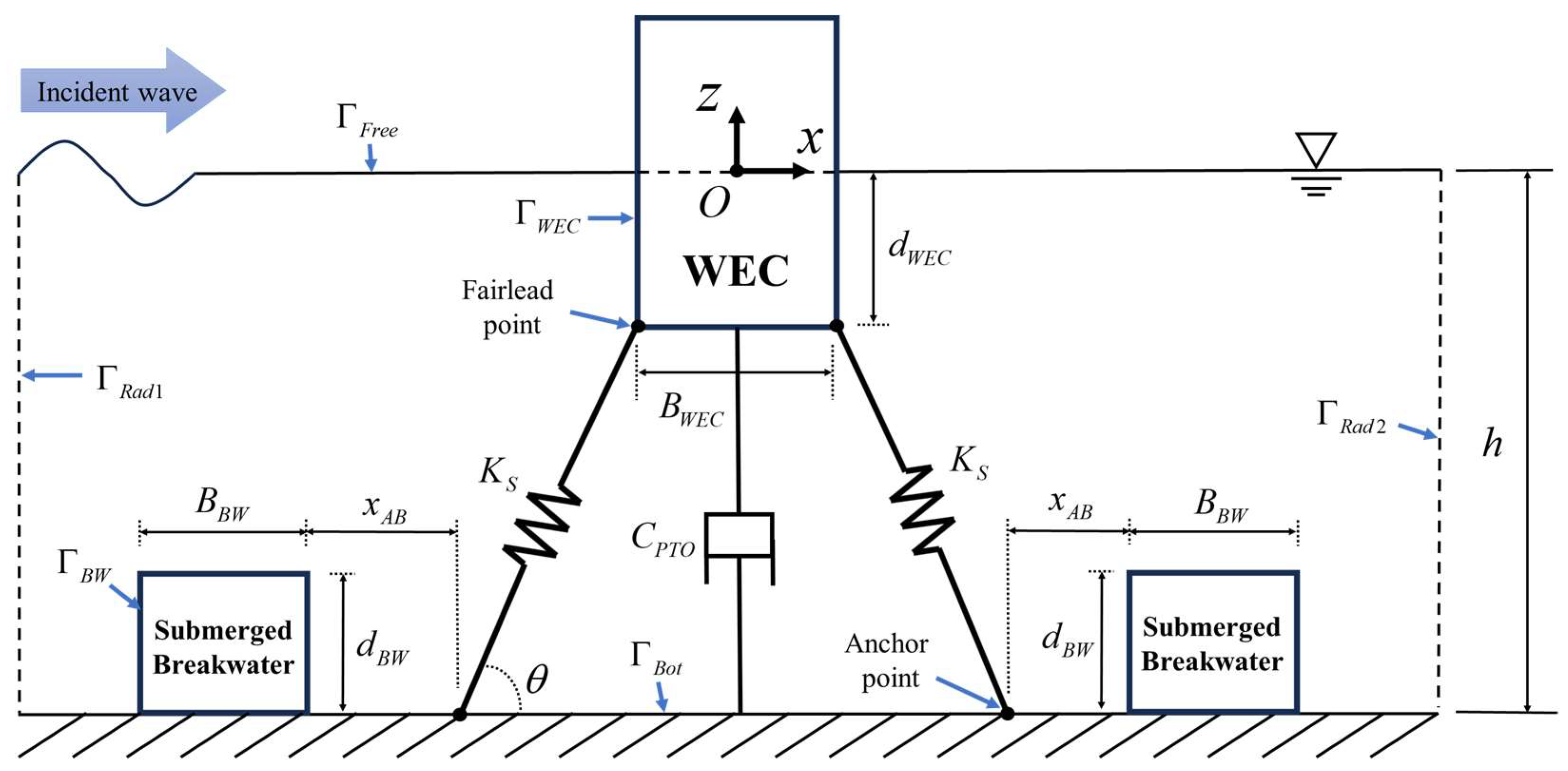
2. Analysis Methods
2.1. FD-BEM
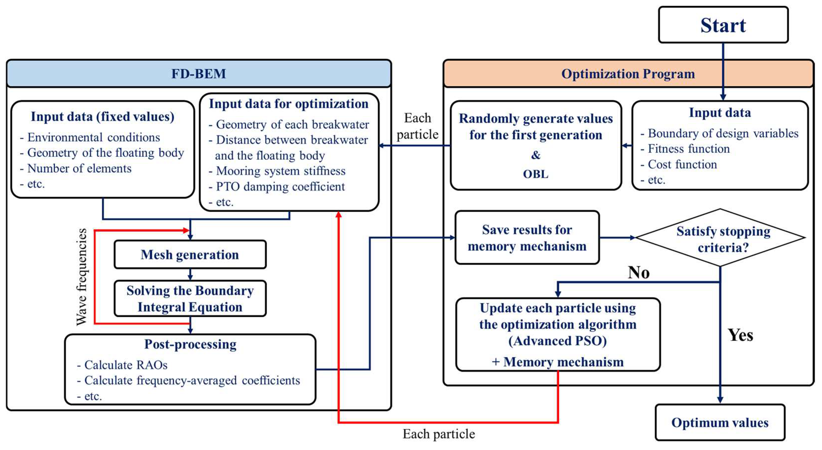
2.2. Metaheuristic Algorithm
3. Numerical Results
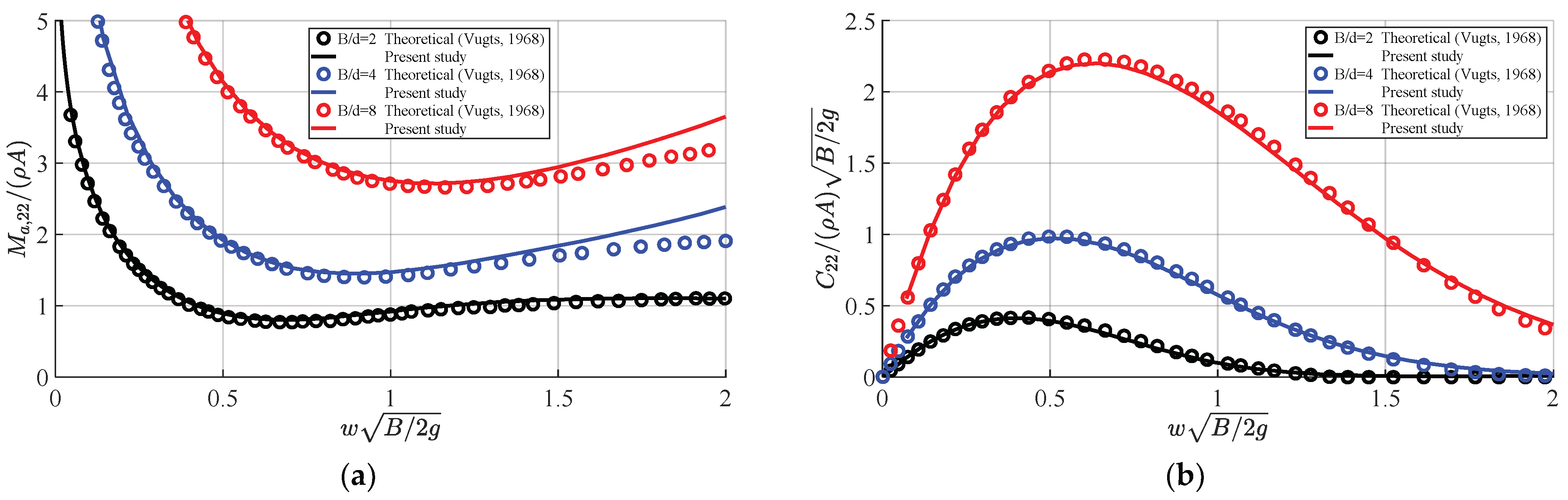
3.1. Validation of the FD-BEM
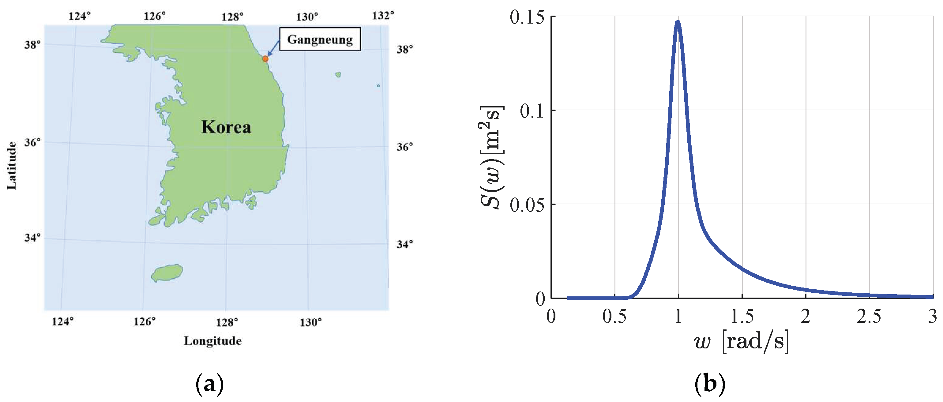
3.2. Irregular Wave Conditions
3.3. Optimization Analysis
4. Conclusions
- Design variables: The study exclusively utilized rectangular shapes for the WEC and submerged breakwaters. Future optimization analyses should consider a variety of shapes to identify more efficient structural configurations.
- Nonlinearity: This study was conducted in a frequency domain based on the linear potential flow theory. Future research should include nonlinear analyses in the time domain to account for nonlinear boundary conditions and external forces.
- Stability of the breakwater: Stability criteria, including considerations of self-weight, buoyancy, and overturning moments acting on the submerged breakwater, should be integrated as constraints in the optimization analysis.
- Applications: This study focused solely on the power production of a WEC. For practical applications, an analysis of the levelized cost of energy (LCOE) should be conducted, taking into account the manufacturing, installation, operation, and maintenance costs of the WEC.
Author Contributions
Funding
Institutional Review Board Statement
Informed Consent Statement
Data Availability Statement
Conflicts of Interest
References
- Jacobson, M.Z.; Delucchi, M.A.; Bauer, Z.A.F.; Goodman, S.C.; Chapman, W.E.; Cameron, M.A.; Bozonnat, C.; Chobadi, L.; Clonts, H.A.; Enevoldsen, P.; et al. 100% Clean and Renewable Wind, Water, and Sunlight All-Sector Energy Roadmaps for 139 Countries of the World. Joule 2017, 1, 108–121. [Google Scholar] [CrossRef]
- Clément, A.; McCullen, P.; Falcão, A.; Fiorentino, A.; Gardner, F.; Hammarlund, K.; Lemonis, G.; Lewis, T.; Nielsen, K.; Petroncini, S.; et al. Wave energy in Europe: Current status and perspectives. Renew. Sustain. Energy Rev. 2002, 6, 405–431. [Google Scholar] [CrossRef]
- Ahamed, R.; McKee, K.; Howard, I. Advancements of Wave Energy Converters Based on Power Take Off (PTO) Systems: A Review. Ocean Eng. 2020, 204, 107248. [Google Scholar] [CrossRef]
- Gaspar, J.F.; Calvário, M.; Kamarlouei, M.; Soares, C.G. Power Take-off Concept for Wave Energy Converters Based on Oil-hydraulic Transformer Units. Renew. Energy 2016, 86, 1232–1246. [Google Scholar] [CrossRef]
- Falcão, A. Wave energy utilization: A review of the technologies. Renew. Sustain. Energy Rev. 2010, 14, 899–918. [Google Scholar] [CrossRef]
- IRENA. Innovation Outlook: Ocean Energy Technologies; International Renewable Energy Agency: Abu Dhabi, United Arab Emirates, 2020. [Google Scholar]
- Guo, B.; Ringwood, J.V. Geometric Optimisation of Wave Energy Conversion Devices: A Survey. Appl. Energy 2021, 297, 117100. [Google Scholar] [CrossRef]
- Guo, B.; Wang, T.; Jin, S.; Duan, S.; Yang, K.; Zhao, Y. A Review of Point Absorber Wave Energy Converters. J. Mar. Sci. Eng. 2022, 10, 1534. [Google Scholar] [CrossRef]
- Ringwood, J.V.; Bacelli, G.; Fusco, F. Energy-maximizing Control of Wave-energy Converters: The Development of Control System Technology to Optimize Their Operation. IEEE Control Syst. Mag. 2014, 34, 30–55. [Google Scholar]
- Mustapa, M.A.; Yaakob, O.B.; Ahmed, Y.M.; Rheem, C.K.; Koh, K.K.; Adnan, F.A. Wave Energy Device and Breakwater Integration: A Review. Renew. Sustain. Energy Rev. 2017, 77, 43–58. [Google Scholar] [CrossRef]
- Kim, T.; Lee, W.D.; Kwon, Y.; Kim, J.; Kang, B.; Kwon, S. Prediction of Wave Transmission Characteristics of Low Crested Structures Using Artificial Neural Network. J. Ocean Eng. Technol. 2022, 36, 313–325. [Google Scholar] [CrossRef]
- Hwang, Y.; Do, K.; Kim, I.; Chang, S. Field observation and Quasi-3D numerical modeling of coastal hydrodynamic response to submerged structures. J. Ocean Eng. Technol. 2023, 37, 68–79. [Google Scholar] [CrossRef]
- Falnes, J. A Review of Wave-energy Extraction. Mar. Struct. 2007, 20, 185–201. [Google Scholar] [CrossRef]
- Zhang, H.; Zhou, B.; Vogel, C.; Willden, R.; Zang, J.; Zhang, L. Hydrodynamic Performance of a Floating Breakwater as an Oscillating-buoy Type Wave Energy Converter. Appl. Energy 2020, 257, 113996. [Google Scholar] [CrossRef]
- Ning, D.; Zhao, X.; Göteman, M.; Kang, H. Hydrodynamic Performance of a Pile-Restrained WEC-Type Floating Breakwater: An Experimental Study. Renew. Energy 2016, 95, 531–541. [Google Scholar] [CrossRef]
- Zhao, X.; Ning, D.; Zhang, C.; Kang, H. Hydrodynamic Investigation of an Oscillating Buoy Wave Energy Converter Integrated into a Pile-restrained Floating Breakwater. Energies 2017, 10, 712. [Google Scholar] [CrossRef]
- Shadman, M.; Estefen, S.F.; Rodriguez, C.A.; Nogueira, I.C. A Geometrical Optimization Method Applied to a Heaving Point Absorber Wave Energy Converter. Renew. Energy 2018, 115, 533–546. [Google Scholar] [CrossRef]
- Reabroy, R.; Zheng, X.; Zhang, L.; Zang, J.; Yuan, Z.; Liu, M.; Sun, K.; Tiaple, Y. Hydrodynamic Response and Power Efficiency Analysis of Heaving Wave Energy Converter Integrated with Breakwater. Energy Convers. Manag. 2019, 195, 1174–1186. [Google Scholar] [CrossRef]
- Zhang, Y.; Li, M.; Zhao, X.; Chen, L. The Effect of the Coastal Reflection on the Performance of a Floating Breakwater-WEC System. Appl. Ocean Res. 2020, 100, 102117. [Google Scholar] [CrossRef]
- Ahmed, A.; Wang, Y.; Azam, A.; Zhang, Z. Design and Analysis of the Bulbous-Bottomed Oscillating Resonant Buoys for an Optimal Point Absorber Wave Energy Converter. Ocean Eng. 2022, 263, 112443. [Google Scholar] [CrossRef]
- He, Z.; Ning, D.; Gou, Y.; Zhou, Z. Wave Energy Converter Optimization Based on Differential Evolution Algorithm. Energy 2022, 246, 123433. [Google Scholar] [CrossRef]
- Nguyen, T.T.D.; Park, J.W.; Yoon, H.K.; Jung, J.C.; Lee, M.M.S. Experimental Study on Application of an Optical Sensor to Measure Mooring-Line Tension in Waves. J. Ocean Eng. Technol. 2022, 36, 153–160. [Google Scholar] [CrossRef]
- Rossell, W.; Ozeren, Y.; Wren, D. Experimental Investigation of a Moored, Circular Pipe Breakwater. J. Waterw. Port Coast. Ocean Eng. 2021, 147, 04021019. [Google Scholar] [CrossRef]
- Guo, W.; Zou, J.; He, M.; Mao, H.; Liu, Y. Comparison of Hydrodynamic Performance of Floating Breakwater with Taut, Slack, and Hybrid Mooring Systems: An SPH-Based Preliminary Investigation. Ocean Eng. 2022, 258, 111818. [Google Scholar] [CrossRef]
- Xu, S.; Wang, S.; Soares, C.G. Review of Mooring Design for Floating Wave Energy Converters. Renew. Sustain. Energy Rev. 2019, 111, 595–621. [Google Scholar] [CrossRef]
- Qiao, D.; Haider, R.; Yan, J.; Ning, D.; Li, B. Review of Wave Energy Converter and Design of Mooring System. Sustainability 2020, 12, 8251. [Google Scholar] [CrossRef]
- Manisha; Kaligatla, R.B.; Sahoo, T. Effect of Bottom Undulation for Mitigating Wave-Induced Forces on a Floating Bridge. Wave Motion 2019, 89, 166–184. [Google Scholar] [CrossRef]
- Vijay, K.G.; Venkateswarlu, V.; Sahoo, T. Bragg Scattering of Surface Gravity Waves by an Array of Submerged Breakwaters and a Floating Dock. Wave Motion 2021, 106, 102807. [Google Scholar] [CrossRef]
- Jiang, L.; Zhang, J.; Tong, L.; Guo, Y.; He, R.; Sun, K. Wave Motion and Seabed Response around a Vertical Structure Sheltered by Submerged Breakwaters with Fabry–Pérot Resonance. J. Mar. Sci. Eng. 2022, 10, 1797. [Google Scholar] [CrossRef]
- Heo, S.; Koo, W.; Kim, M. Optimization Analysis of the Shape and Position of a Submerged Breakwater for Improving Floating Body Stability. J. Ocean Eng. Technol. 2024, 38, 53–63. [Google Scholar] [CrossRef]
- Chen, K.; Zhou, F.; Yin, L.; Wang, S.; Wang, Y.; Wan, F. A Hybrid Particle Swarm Optimizer with Sine Cosine Acceleration Coefficients. Inf. Sci. 2018, 422, 218–241. [Google Scholar] [CrossRef]
- Jeong, H.J.; Koo, W. Analysis of Various Algorithms for Optimizing the Wave Energy Converters Associated with a Sloped Wall-Type Breakwater. Ocean Eng. 2023, 276, 114199. [Google Scholar] [CrossRef]
- Kim, M.H.; Koo, W.C.; Hong, S.Y. Wave interactions with 2D structures on/inside porous seabed by a two-domain boundary element method. Appl. Ocean Res. 2000, 22, 255–266. [Google Scholar] [CrossRef]
- Nakos, D.E. Ship Wave Patterns and Motions by a Three-Dimensional Rankine Panel Method. Ph.D. Thesis, Massachusetts Institute of Technology, Cambridge, MA, USA, 1990. [Google Scholar]
- Lee, C.H. WAMIT Theory Manual. Report No. 95-2; Department of Ocean Engineering, Massachusetts Institute of Technology: Cambridge, MA, USA, 1995. [Google Scholar]
- Folley, M. (Ed.) Numerical Modelling of Wave Energy Converters: State-of-the-Art Techniques for Single Devices and Arrays; Academic Press: Cambridge, MA, USA, 2016. [Google Scholar]
- Koh, H.J.; Ruy, W.S.; Cho, I.H.; Kweon, H.M. Multi-Objective Optimum Design of a Buoy for the Resonant-Type Wave Energy Converter. J. Mar. Sci. Technol. 2015, 20, 53–63. [Google Scholar] [CrossRef]
- Tom, N.M.; Lawson, M.J.; Yu, Y.H.; Wright, A.D. Development of a Nearshore Oscillating Surge Wave Energy Converter with Variable Geometry. Renew. Energy 2016, 96, 410–424. [Google Scholar] [CrossRef]
- Koley, S.; Panduranga, K.; Almashan, N.; Neelamani, S.; Al-Ragum, A. Numerical and Experimental Modeling of Water Wave Interaction with Rubble Mound Offshore Porous Breakwaters. Ocean Eng. 2020, 218, 108218. [Google Scholar] [CrossRef]
- He, F.; Huang, Z. Hydrodynamic Performance of Pile-Supported OWC-Type Structures as Breakwaters: An Experimental Study. Ocean Eng. 2014, 88, 618–626. [Google Scholar] [CrossRef]
- Goda, Y. A Comparative Review on the Functional Forms of Directional Wave Spectrum. Coast. Eng. J. 1999, 41, 1–20. [Google Scholar] [CrossRef]
- Pastor, J.; Liu, Y. Power Absorption Modeling and Optimization of a Point Absorbing Wave Energy Converter Using Numerical Method. J. Energy Resour. Technol. 2014, 136, 021207. [Google Scholar] [CrossRef]
- Goda, Y. Random Seas and Design of Maritime Structures, 3rd ed.; World Scientific Co Pte. Ltd.: Tokyo, Japan, 2010. [Google Scholar]
- Eberhart, R.; Kennedy, J. A New Optimizer Using Particle Swarm Theory. In MHS’95. Proceedings of the Sixth International Symposium on Micro Machine and Human Science, Nagoya, Japan, 4–6 October 1995; pp. 39–43. [Google Scholar]
- Shami, T.M.; El-Saleh, A.A.; Alswaitti, M.; Al-Tashi, Q.; Summakieh, M.A.; Mirjalili, S. Particle swarm optimization: A comprehensive survey. IEEE Access 2022, 10, 10031–10061. [Google Scholar] [CrossRef]
- Shi, Y.; Eberhart, R.C. Parameter Selection in Particle Swarm Optimization. In Proceedings of the Evolutionary Programming VII: 7th International Conference, EP98, San Diego, CA, USA, 25–27 March 1998; Springer: Berlin/Heidelberg, Germany, 1998; pp. 591–600. [Google Scholar]
- Ahandani, M.A. Opposition-Based Learning in the Shuffled Bidirectional Differential Evolution Algorithm. Swarm Evol. Comput. 2016, 26, 64–85. [Google Scholar] [CrossRef]
- Cao, F.; Han, M.; Shi, H.; Li, M.; Liu, Z. Comparative Study on Metaheuristic Algorithms for Optimising Wave Energy Converters. Ocean Eng. 2022, 247, 110461. [Google Scholar] [CrossRef]
- Vugts, J.H. The hydrodynamic coefficients for swaying, heaving, and rolling cylinders in a free surface. Int. Shipbuild. Prog. 1968, 15, 251–276. [Google Scholar] [CrossRef]
- Jeong, W.M.; Oh, S.H.; Ryu, K.H.; Back, J.D.; Choi, I.H. Establishment of Wave Information Network of Korea (WINK). J. Korean Soc. Coast. Ocean Eng. 2018, 30, 326–336. [Google Scholar] [CrossRef]
- WINK. Wave Information Network of Korea (WINK). Available online: http://wink.go.kr/map/map.do (accessed on 4 March 2024).
- Guth, S.; Katsidoniotaki, E.; Sapsis, T.P. Statistical Modeling of Fully Nonlinear Hydrodynamic Loads on Offshore Wind Turbine Monopile Foundations Using Wave Episodes and Targeted CFD Simulations through Active Sampling. Wind. Energy 2024, 27, 75–100. [Google Scholar] [CrossRef]
- Falnes, J.; Lillebekken, P.M. Budal’s latching-controlled-buoy type wave-power plant. In Proceedings of the Fifth European Wave Energy Conference, Cork, Ireland, 17–20 September 2003; pp. 233–244. [Google Scholar]
- Katsidoniotaki, E.; Göteman, M. Numerical Modeling of Extreme Wave Interaction with Point-Absorber Using OpenFOAM. Ocean Eng. 2022, 245, 110268. [Google Scholar] [CrossRef]
- Liu, Y.; Yue, D.K. On Generalized Bragg Scattering of Surface Waves by Bottom Ripples. J. Fluid Mech. 1998, 356, 297–326. [Google Scholar] [CrossRef]


| Description | Value |
|---|---|
| Width (BWEC) | 5.1 m |
| Draft (dWEC) | 10.2 m |
| Overall length | 20.4 m |
| Submerged area (AWEC) | 52.02 m2 |
| Center of gravity | (0, 0) |
| Mass | 53,320.5 kg |
| Moment of inertia | 1,964,727 kg·m2 |
| Heave stiffness (K22) | 51,260.9 N/m |
| Fairlead points | (±2.55, −10.2) m |
| Anchor points | (±7.65, −34) m |
| Design Variables | Lower Limit | Upper Limit | Step Size |
|---|---|---|---|
| [Ns/m] | 100 | 30,000 | 100 |
| [N/m] | 100 | 15,000 | 100 |
| 0.0 | 20.0 | 0.1 | |
| 1.0 | 15.0 | 0.1 | |
| 0.3 | 0.8 | 0.01 |
| Components | Description |
|---|---|
| CPU | Intel (R) Xeon (R) Platinum 8260 (2.40 GHz) |
| Cores of CPU | 48 |
| RAM | 192 GB |
| OS | Windows 10 |
| Compiler | Intel® Fortran Compiler Classic 2021.8.0 [Intel(R) 64] |
| Cases | Total Simulation Time [h] | Converged Iteration | Total Number of Simulations |
|---|---|---|---|
| Case 1 | 3.37 | 152 | 3354 |
| Case 2 | 40.29 | 197 | 36,939 |
| Case 3 | 30.46 | 213 | 26,504 |
| Case 4 | 33.65 | 242 | 26,938 |
| Parameters | Case 1 | Case 2 | Case 3 | Case 4 | |
|---|---|---|---|---|---|
| Optimized design variables | CPTO [Ns/m] | 5700 | 6200 | 7600 | 13,700 |
| KS [N/m] | 7500 | 7700 | 8800 | 12,400 | |
| xab/BWEC | - | 1.7 | 0.0 | 0.0 | |
| ARatio(=ABW/AWEC) | - | 2.5 | 11.6 | 12.3 | |
| dBW/h | - | 0.8 | 0.8 | 0.8 | |
| Corresponding parameters | BBW(=ABW/dBW) [m] | - | 4.78 | 22.19 | 20.85 |
| CPTO,opt(ωP) [Ns/m] | 2825 | 2796 | 4241 | 11,178 | |
| Cases | CWR | ||
|---|---|---|---|
| Case 1 | 2.95 × 10⁻² (1.00) | 0.484 (1.000) | 0.791 (1.000) |
| Case 2 | 3.54 × 10⁻² (1.20) | 0.487 (1.006) | 0.772 (0.975) |
| Case 3 | 5.30 × 10⁻² (1.80) | 0.461 (0.953) | 0.734 (0.928) |
| Case 4 | 5.88 × 10⁻² (1.99) | 0.499 (1.030) | 0.687 (0.868) |
Disclaimer/Publisher’s Note: The statements, opinions and data contained in all publications are solely those of the individual author(s) and contributor(s) and not of MDPI and/or the editor(s). MDPI and/or the editor(s) disclaim responsibility for any injury to people or property resulting from any ideas, methods, instructions or products referred to in the content. |
© 2024 by the authors. Licensee MDPI, Basel, Switzerland. This article is an open access article distributed under the terms and conditions of the Creative Commons Attribution (CC BY) license (https://creativecommons.org/licenses/by/4.0/).
Share and Cite
Heo, S.; Koo, W. Optimization of Submerged Breakwaters for Maximum Power of a Point-Absorber Wave Energy Converter Using Bragg Resonance. J. Mar. Sci. Eng. 2024, 12, 1107. https://doi.org/10.3390/jmse12071107
Heo S, Koo W. Optimization of Submerged Breakwaters for Maximum Power of a Point-Absorber Wave Energy Converter Using Bragg Resonance. Journal of Marine Science and Engineering. 2024; 12(7):1107. https://doi.org/10.3390/jmse12071107
Chicago/Turabian StyleHeo, Sanghwan, and Weoncheol Koo. 2024. "Optimization of Submerged Breakwaters for Maximum Power of a Point-Absorber Wave Energy Converter Using Bragg Resonance" Journal of Marine Science and Engineering 12, no. 7: 1107. https://doi.org/10.3390/jmse12071107