Seasonal Variation of Submesoscale Ageostrophic Motion and Geostrophic Energy Cascade in the Kuroshio

Abstract

The study of submesoscale ageostrophic motion is crucial for enhancing our comprehension of ocean dynamics. This paper employs global sea surface velocity reanalysis data and mixed layer depth data to examine the factors influencing submesoscale ageostrophic energy in the Kuroshio region as well as the energy transition between ageostrophic and geostrophic energy. The findings indicate that submesoscale ageostrophic kinetic energy in the Kuroshio region peaks during winter and spring. Mixed layer depth and geostrophic strain significantly boost ageostrophic kinetic energy, especially in strong current area. Analysis of kinetic energy spectral density reveals how energy distribution and transition scale vary across strong and slow current zones during different seasons, highlighting that submesoscale kinetic energy is susceptible to seasonal variations. In summer and autumn, the transition scale of kinetic energy is generally larger compared to those in spring and winter. Submesoscale ageostrophic motion predominantly gains kinetic energy from the release of available potential energy (APE) and horizontal shear production (HSP) while losing a small portion of its kinetic energy through vertical shear production (VSP) in the Kuroshio.

1. Introduction

The approximate scale range of submesoscale flow is 1–50 km horizontally and 1–10 days in time [1]. This occurs when the geostrophic equilibrium is not maintained, leading to significant ageostrophic motion and positive energy cascades to smaller scales. Submesoscale ageostrophic motions encompass a wide range of dynamic processes, including Ekman advection, tides, inertial motion, current straining, and frontogenesis [2,3,4,5]. Submesoscale motion is found to enhance water exchange between the mixed layer and the ocean interior, playing a vital role in nutrient transport, phytoplankton growth, and heat balance [6,7,8,9,10,11,12,13,14]. Moreover, submesoscale processes also interact with small-scale turbulence, influencing the distribution and transport of ocean energy through energy transfer and dissipation processes [15,16,17,18,19,20,21].

Bo Qiu et al. explored the scale interaction in the ocean, evaluated the length scale (LS) between inverse and forward cascades in various ocean regions, and analyzed Acoustic Doppler Current Profiler (ADCP) survey data conducted by the Japan Meteorological Agency along the 165° E meridian, shedding light on the processes leading to different LS values. Their findings suggest that LS varies across different ocean regions and is influenced by the characteristics of the background circulation and eddy variability [22]. Zhang Z et al. investigated the impact of geostrophic strain on ageostrophic motions and surface chlorophyll concentrations and highlighted the significant influence of geostrophic strain and submesoscale ageostrophic processes on near-surface chlorophyll variations in the ocean. This underscores the importance of these processes in understanding variations in oceanic chlorophyll and their implications for the carbon cycle and ecosystem dynamics. Furthermore, Zhang Z et al. found that the evolution of submesoscale ageostrophic motions is closely linked to the life cycle of oceanic mesoscale eddies. They observed that the strain rate, a measure of deformation, is high during the formation and decay phases of the eddies and low during the mature phase [23]. However, there has been little quantitative analysis of submesoscale ageostrophic energy cascades in the Kuroshio region by previous researchers.

In this study, we conducted a quantitative analysis of the correlation between submesoscale ageostrophic motion and geostrophic strain, the mixed layer in the Kuroshio region, utilizing satellite altimeter data, and delved into seasonal variations in kinetic energy spectral density and the transitional scale between geostrophic and submesoscale ageostrophic flows. Moreover, we researched the kinetic energy transfer rate between geostrophic and submesoscale ageostrophic flows in the Kuroshio region.

2. Materials and Methods

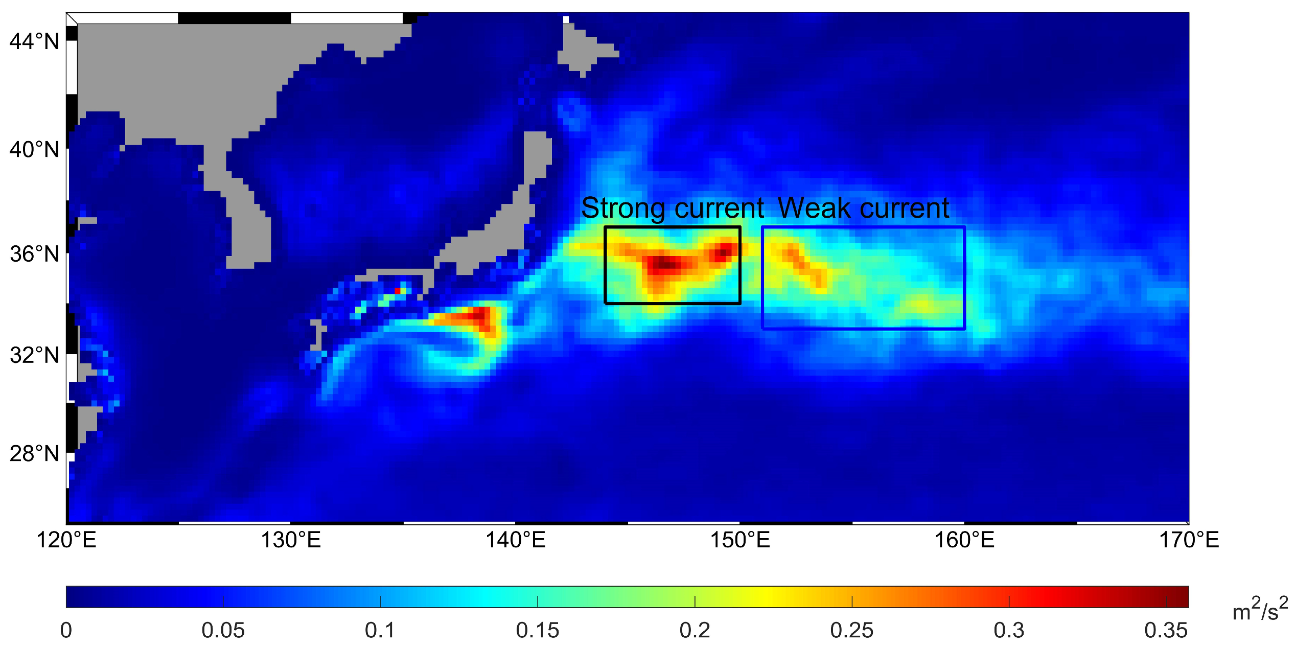
2.1. Study Area

Figure 1 illustrates the distribution of mesoscale geostrophic energy in the Kuroshio region (20–60° N, 120–180° E), which is categorized into areas of strong and weak currents based on kinetic energy levels. The Kuroshio, also known as the Japan Current, is a significant and stable warm current in the western Pacific. It is distinguished not only by its unique geographical features but also by its critical role in the global ocean circulation system [24]. Originating in the Philippine Sea, it travels along the eastern coasts of the Philippines, Taiwan, and Japan before merging into the vast Pacific Ocean. The warm current moderates the climate of the coastal countries and profoundly influences their local marine ecosystems.

The warm current properties of the Kuroshio significantly influence the climate along the East Asian coast, particularly by providing relatively warm winters and cool summers in Japan. The heat and salt transports of the Kuroshio play a critical role in the global climate system by facilitating the redistribution of Earth’s heat and salt [25]. The ecological significance of the Kuroshio is equally noteworthy. It furnishes rich food sources and suitable habitats for marine life, offering nutrient-rich waters that sustain numerous fish species and other marine organisms [26,27,28]. Due to its transportation of warm waters from the tropics, the Kuroshio current supports diverse and unique biological communities, essential for maintaining and enhancing biodiversity [29,30,31]. Through extensive observation and research, scientists have acquired a deep understanding of the Kuroshio’s dynamic characteristics and its transport of heat, salt, and nutrients [32]. In Earth system science, studying how the Kuroshio current interacts with other ocean currents, particularly its effects on the balance of global marine ecosystems, is a vital research domain [33,34,35]. Variations in the physical properties of the Kuroshio influence not only the surface ocean but also extend deep into the ocean, contributing to the formation of deep water and global deep-sea circulation [36,37,38]. Given the current global climate change, researching the Kuroshio has become increasingly imperative. As Earth’s surface temperatures rise, the Kuroshio’s strength, path, and water properties might be altered, potentially impacting global climate [39,40,41]. These changes could alter precipitation patterns, affect the intensity and frequency of storms, and modify the dynamics of global marine ecosystems [42]. Hence, the Kuroshio serves not merely as a sea current but also as a crucial regulator within the Earth system.

2.2. Data and Methods

2.2.1. Velocity Data

The geostrophic current anomaly velocities and the total current velocity from 2012 to 2020 were retrieved from the Copernicus Marine Environment Monitoring Service (CMEMS) website. These datasets are merged products originating from various altimeter missions including Topography Experiment (TOPEX) Poseidon (T/P), Jason-1/2 (French–US altimeter satellites), ERS-1/2 (European Remote Sensing satellites), and Envisat (European Remote Sensing satellite). The gridded data have undergone geophysical and meteorological corrections and have been interpolated onto Mercator grids with a (1/12)° horizontal resolution, covering global oceans except for high latitude regions. The data have a temporal resolution of one day, covering the period from 1 January 1993 to 26 March 2024. These data are employed to calculate geostrophic energy, the kinetic energy of submesoscale and geostrophic strain.

The MITgcm model LLC4320 data from 10 September 2011 to 15 November 2012 are used in this study, driven by wind fields from the European Centre for Medium-Range Weather Forecasts (ECMWF) every 6 h. The model can effectively simulate multi-scale dynamical processes such as mesoscale eddies, submesoscale processes, near-inertial motions, and internal tides. The model outputs physical quantities including sea surface height (SSH), horizontal (u, v) and vertical velocities (w), wind stress, temperature, and salinity. The data have a horizontal resolution of 1/48° (approximately 2 km), a vertical division into 90 layers, and a temporal resolution of 1 h, which are used to calculate kinetic energy spectrum and kinetic energy transfer rate.

2.2.2. Mixed Layer Depth Data

The mixed layer depth (MLD) data, provided as grid data by the Copernicus Marine Environment Monitoring Service, feature a spatial resolution of 0.25° and a temporal resolution of one day.

2.2.3. Calculation of Geostrophic and Ageostrophic Energy

The total velocity $\mathrm{U}$ includes all velocity components caused by various dynamic processes. Here, we decompose the total velocity at each grid $\mathrm{U}$ into two components:

$${\mathrm{U}}_{age}\left(\mathrm{i},\mathrm{j},\mathrm{t}\right)=\mathrm{U}\left(\mathrm{i},\mathrm{j},\mathrm{t}\right)-{\mathrm{U}}_{ge}\left(i,j,t\right)$$

(1)

where $\mathrm{i},\mathrm{j}$ are the zonal and meridional grids, respectively, and $\mathrm{t}$ is the time. Considering that submesoscale processes contain significant ageostrophic kinetic energy, the geostrophic velocity ${\mathrm{U}}_{ge}$ is calculated using a 15-day low-pass filter on the original velocity. Since the typical time scale of oceanic submesoscale processes is about 1–10 days, we set the cutoff period of our high-pass filter to 7 days. This period is longer than most unbalanced submesoscale ageostrophic motions but significantly shorter than the typical evolution time scale of mesoscale eddies. By applying the high-pass filter, we use a 2–7 day band-pass filter for ${\mathrm{U}}_{age}$ and define the 2–7 day ageostrophic velocity ${\mathrm{U}}_{age}$ as submesoscale ageostrophic velocity in the analysis that follows [1]. The geostrophic kinetic energy ${\mathrm{E}}_{\mathrm{ga}}$ and ageostrophic kinetic energy ${\mathrm{E}}_{\mathrm{age}}$ calculation is as follows [43]:

$${\mathrm{E}}_{\mathrm{ga}}=\frac{{\left|U_{ge}\left(i,j,t\right)\right|}^2}{2}$$

(2)

$${\mathrm{E}}_{\mathrm{age}}=\frac{{\left|U_{age}\left(i,j,t\right)\right|}^2}{2}$$

(3)

2.2.4. Geostrophic Strain

The data employed to calculate the geostrophic strain originate from the geostrophic current anomaly provided by the satellite altimeter (AVISO). The formula used for this calculation is as follows [44]:

$$\mathrm{MSR}={\left({\left({\mathrm{u}}_{\mathrm{x}}-{\mathrm{v}}_{\mathrm{y}}\right)}^2+{\left({\mathrm{v}}_{\mathrm{x}}+{\mathrm{u}}_{\mathrm{y}}\right)}^2\right)}^{1/2}$$

(4)

MSR denotes geostrophic strain rate and $\mathrm{u}$ and $\mathrm{v}$ represent geostrophic velocity anomalies.

2.2.5. Kinetic Energy Spectral Density

To calculate the kinetic energy spectral density, the study area was initially divided into 10 overlapping subregions, each measuring 8° × 8° and comprising 128 × 128 grids. The daily current velocity data for each subregion are first detrended by subtracting a linear plane fitted using the least squares method and then smoothed using the Hanning window in preparation for the Discrete Fourier Transform (DFT). The kinetic energy spectral density is subsequently calculated using the formula provided below [22].

$$\mathrm{E}\left({\mathrm{k}}_{\mathrm{x}},{\mathrm{k}}_{\mathrm{y}},\mathrm{t}\right)=\frac{1}{2}\left(\hat{\mathrm{u}}{\hat{\mathrm{u}}}^{*}+\hat{\mathrm{v}}{\hat{\mathrm{v}}}^{*}\right)/{\mathsf{\Delta }\mathrm{k}}^2$$

(5)

$\mathsf{\Delta }\mathrm{k}=1/\left(\mathrm{N}\mathsf{\Delta }\mathrm{x}\right)$, with the unit of weeks/km, where $\mathsf{\Delta }\mathrm{x}$ represents the grid length, N = 32 denotes the number of grid points in each direction, and $\hat{\mathrm{u}}, \hat{\mathrm{v}},$ respectively, are the Fourier transforms of ${\mathrm{u}}_{\mathrm{g}}$, ${\mathrm{v}}_{\mathrm{g}}$. The complex conjugates are denoted as ${\hat{\mathrm{u}}}^{*}, {\hat{\mathrm{v}}}^{*}$. The zonal and meridional wave number $\left({\mathrm{k}}_{\mathrm{x}},{\mathrm{k}}_{\mathrm{y}}\right)=2\pi \left(\mathrm{m}/{\mathrm{L}}_{\mathrm{x}},\mathrm{n}/{\mathrm{L}}_{\mathrm{y}}\right)$, where m and n range from [−16, 16].

2.2.6. Kinetic Energy Transfer Rate

In conditions where there is no wind forcing on the sea surface, horizontal shear production (HSP) and vertical shear production (VSP) and baroclinic conversion (BC) serve as potential energy sources for the vortex [45,46]. The formula for this calculation is as follows:

$$\mathrm{HSP}=-\left(\overline{{\mathrm{u}}^{\prime }{\mathrm{v}}^{\prime }}\frac{\partial \stackrel{-}{\mathrm{U}}}{\partial \mathrm{y}}+\overline{{\mathrm{u}}^{\prime }{\mathrm{u}}^{\prime }}\frac{\partial \stackrel{-}{\mathrm{U}}}{\partial \mathrm{x}}+\overline{{\mathrm{u}}^{\prime }{\mathrm{v}}^{\prime }}\frac{\partial \stackrel{-}{\mathrm{V}}}{\partial \mathrm{x}}+\overline{{\mathrm{v}}^{\prime }{\mathrm{v}}^{\prime }}\frac{\partial \stackrel{-}{\mathrm{V}}}{\partial \mathrm{y}}\right)$$

(6)

$$\mathrm{VSP}=-\left(\overline{{\mathrm{u}}^{\prime }{\mathrm{w}}^{\prime }}\frac{\partial \stackrel{-}{\mathrm{V}}}{\partial \mathrm{Z}}+\overline{{\mathrm{v}}^{\prime }{\mathrm{w}}^{\prime }}\frac{\partial \stackrel{-}{\mathrm{U}}}{\partial \mathrm{Z}}\right)$$

(7)

The submesoscale ageostrophic velocities ${\mathrm{u}}^{\prime }$, ${\mathrm{v}}^{\prime },$ and ${\mathrm{w}}^{\prime }$ are derived using a 2–7-day band-pass filter. $\stackrel{-}{\mathrm{U}}$ and $\stackrel{-}{\mathrm{V}}$ represent the geostrophic velocities. If the kinetic energy transfer rate is positive, it indicates that kinetic energy is being transferred from ocean geostrophic motion to ocean submesoscale ageostrophic motion through shear. Conversely, if the kinetic energy transfer rate is negative, it signifies an inverse cascade of kinetic energy transfer from ageostrophic motion to geostrophic motion through shear.

$$BC=-\frac{g}{{\rho }_0}\overline{w^{\prime }{\rho }^{\prime }}$$

(8)

where $g=9.8\mathrm{m}/{\mathrm{s}}^2$ represents the gravitational acceleration, ${\rho }_0=1030\mathrm{kg}/{\mathrm{m}}^3$ is the reference density, and $w^{\prime }$ and ${\rho }^{\prime }$ denote the submesoscale vertical velocity and potential density anomalies, respectively, which are calculated using a 2–7 day band-pass filter. Dynamically, the BC term corresponds to the submesoscale vertical buoyancy flux [47,48]. A positive $\mathrm{BC}$ value indicates the rate at which available potential energy (APE) is converted to submesoscale kinetic energy (KE) due to baroclinic instability.

3. Results and Discussion

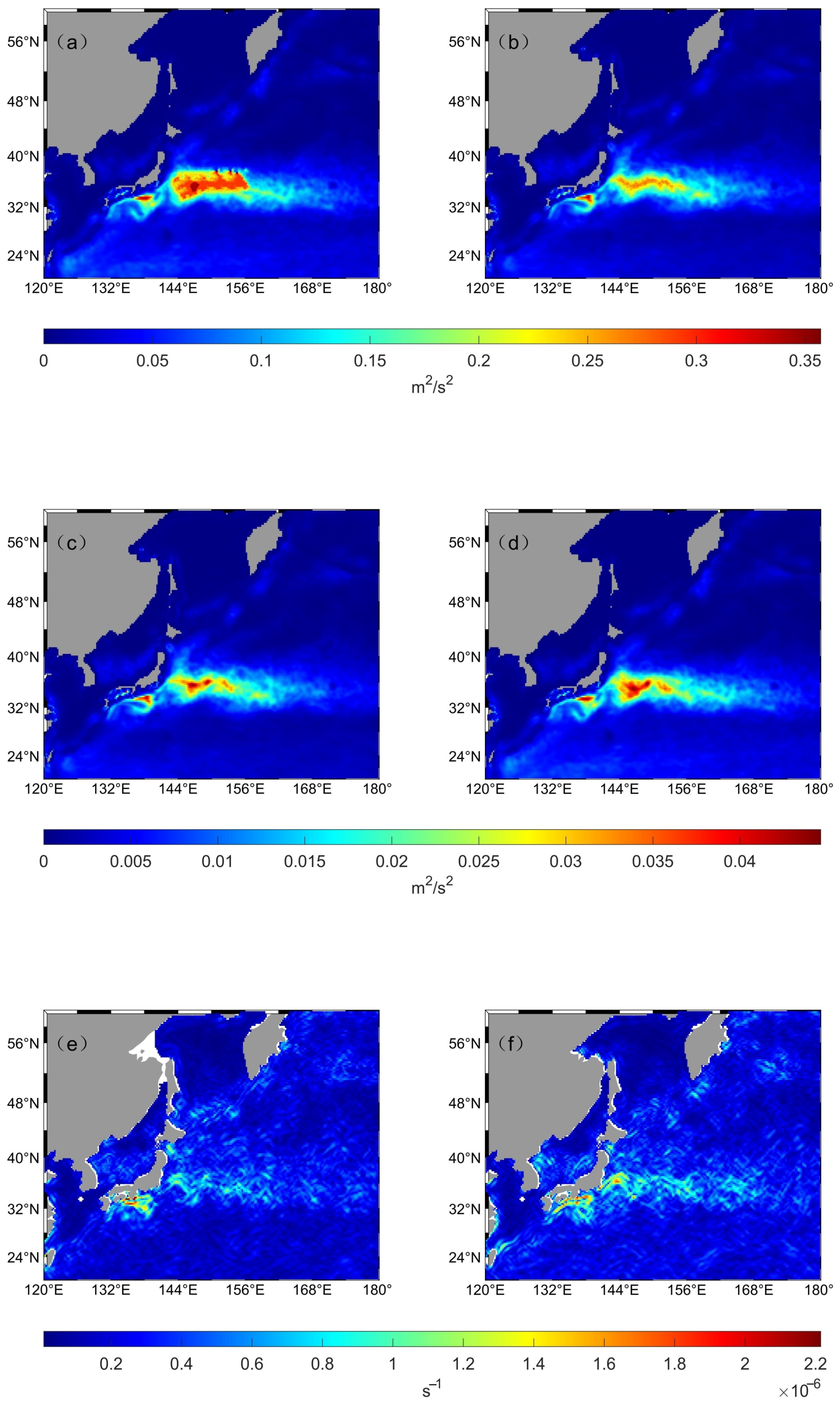
3.1. Analysis of Seasonal Variation of Ocean Submesoscale Ageostrophic Motion

Figure 2 illustrates the distribution of geostrophic kinetic energy, submesoscale ageostrophic kinetic energy, and geostrophic strain in the Kuroshio region (20–60° N, 120–180° E) during summer and autumn (Figure 2a,c,e) and winter and spring (Figure 2b,d,f). According to Figure 3c,d, submesoscale ageostrophic kinetic energy is higher in winter and spring than in summer and autumn. Conversely, geostrophic kinetic energy in the Kuroshio is stronger in summer and autumn and weaker in winter and spring (Figure 2a,b). Although the energies display different trends, they both show that areas of high submesoscale ageostrophic motion correspond to areas of high geostrophic energy, which suggests that the formation of submesoscale ageostrophic motion in the ocean is closely linked to the presence of strong currents and mesoscale vortices. The geostrophic strain variability exhibits seasonal differences in the Kuroshio (Figure 2e,f). During winter and spring, increased geostrophic strain, driven by strong winds and vortices, leads to enhanced vertical mixing and upward nutrient transport. In contrast, the lower geostrophic strain in summer and autumn aligns with a more stable state of the surface ocean. Overall, the patterns in winter and spring are stronger than those in summer and autumn. The distribution of high-value regions also aligns with ageostrophic energy, further indicating a strong correlation between submesoscale ageostrophic kinetic energy and frontogenesis, which aligns with Schubert et al.’s observations of a kinetic energy cascade towards larger scales during these seasons [16].

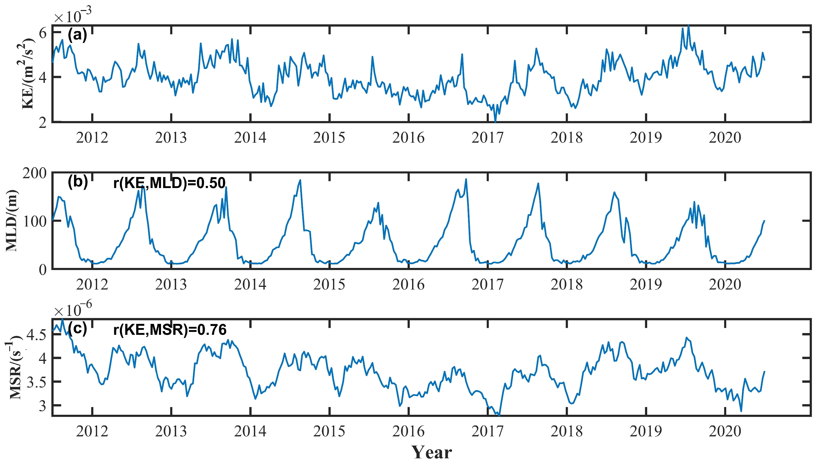
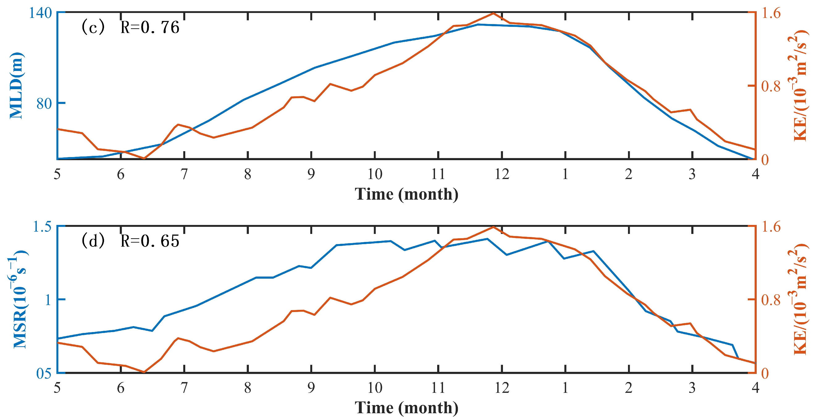
3.2. Relationship between Ageostrophic Submesoscale Motions, Geostrophic Strain, and Mixed Layer Depth

Previous studies have demonstrated that mixed layer instability is a significant factor influencing submesoscale ageostrophic motion, with its impact largely dependent on MLD [47,48]. This study quantitatively examines the relationship between submesoscale ageostrophic kinetic energy (KE), geostrophic strain (MSR), and MLD. The findings reveal that the mixed layer typically deepens in winter due to increased vertical mixing, prompted by lower temperatures and stronger winds. Conversely, it becomes shallower in summer, resulting from stratification due to rising ocean surface temperatures. Submesoscale KE shows a strong correlation with MSR (Figure 3c), evidenced by a correlation coefficient (R) of 0.76 (95% confidence interval), which is significantly higher than its correlation with MLD (Figure 3b, R = 0.50, 95% confidence interval). Schubert et al.’s findings also support the notion that enhanced vertical mixing and the absorption of mixed-layer eddies by mesoscale eddies are key processes driving these seasonal trends [49].

Figure 3. Time series of average submesoscale KE (a), mixed layer depth MLD (b), and geostrophic strain MSR (c) above 150 m.

Figure 3. Time series of average submesoscale KE (a), mixed layer depth MLD (b), and geostrophic strain MSR (c) above 150 m.

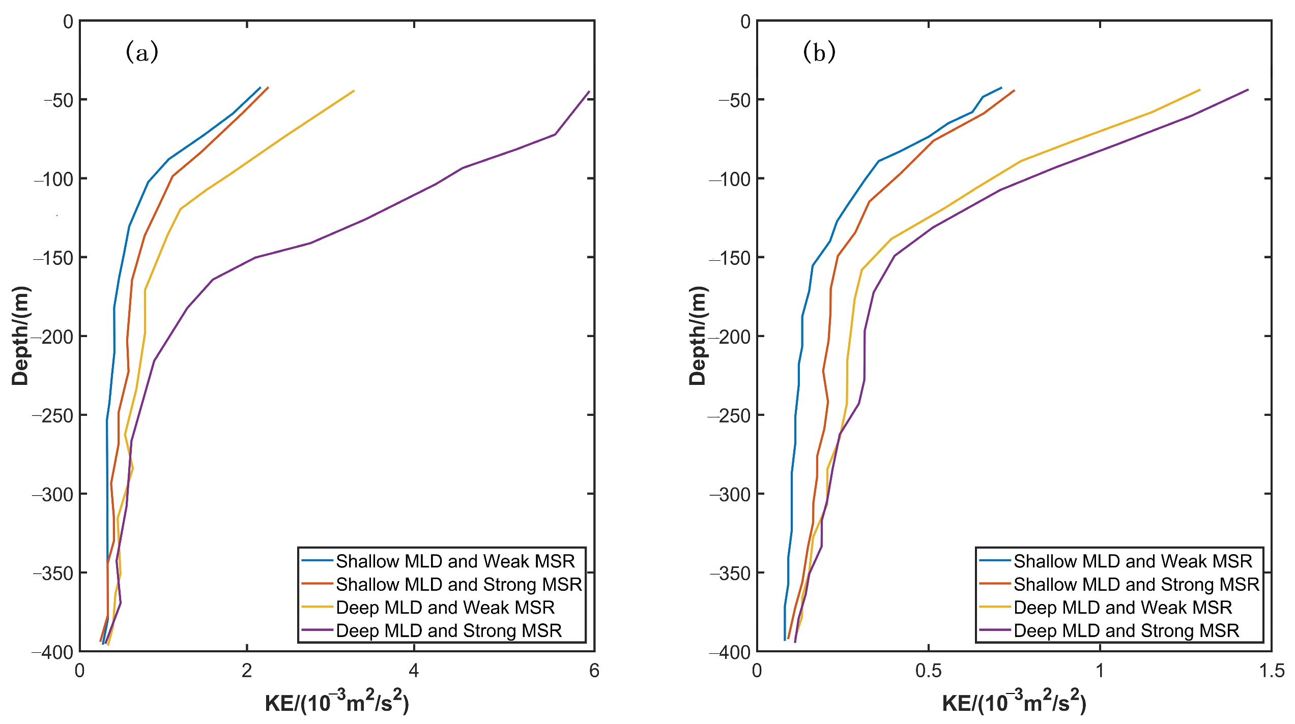
3.3. Vertical Changes in Submesoscale KE under Different Conditions

To compare the effects of MLD and MSR on submesoscale ageostrophic energy, the study analyzed energy curves from four distinct scenarios within the Kuroshio region (Figure 4): (1) shallow MLD and weak MSR, (2) shallow MLD and strong MSR, (3) deep MLD and weak MSR, (4) deep MLD and strong MSR. Strong and weak MSR and deep and shallow MLD are quantified as values 20% greater or less than the average, respectively [44]. Notably, the depths categorized as deep and shallow MLD typically occur in spring and winter, and summer and autumn, respectively. In contrast, the seasonal variations corresponding to strong and weak MSR are less pronounced.

Submesoscale ageostrophic energy is lowest when the MLD is shallow and the MSR is weak, with slightly higher levels observed when the MLD is shallow and MSR is strong. In regions with strong currents, submesoscale ageostrophic energy demonstrates greater sensitivity to MLD compared to MSR. Under varying conditions of geostrophic strain and mixed layer depths, the lowest ageostrophic energy levels consistently occur with shallow MLD and weak MSR. In areas of slow current, the impact of changes in MSR on submesoscale ageostrophic energy is more constrained due to inherently lower kinetic energy, making the energy increases driven by MSR less pronounced compared to those in strong current areas. Comparison of Figure 4a,b shows that ageostrophic energy induced by MSR in areas with strong currents is significantly higher than in areas with slow currents. Moreover, an increase in MSR, particularly in shallow mixed layers, markedly enhances peak ageostrophic energy. These findings suggest that a deeper mixing layer in the Kuroshio is essential for generating significant submesoscale ageostrophic energy and that mixing layer instability has a more substantial influence than geostrophic strain.

Figure 5 displays the average time series of submesoscale ageostrophic energy correlated with MLD and MSR for ocean depths above 150 m. There is a strong correlation between the seasonal variations of submesoscale ageostrophic energy in the Kuroshio’s strong and slow current regions with MLD and MSR, achieving correlation coefficients (R) of 0.85, 0.71 and 0.76, 0.65 (95% confidence level), respectively. In the strong current regions of the Kuroshio (Figure 5a), submesoscale ageostrophic energy and MLD exhibit similar seasonal patterns, and the correlation between submesoscale ageostrophic KE and MSR is particularly high from December to March, while it diminishes during other months (Figure 5b), and the peak of MSR corresponds to the peak of KE (Figure 5a,b). In the slow current areas (Figure 5c,d), although the correlation between submesoscale ageostrophic energy, MLD, and MSR is somewhat lower than in the strong current areas, it still displays significant seasonal trends and maintains a robust correlation. Overall, it can be concluded that the general seasonal patterns of submesoscale ageostrophic energy in the Kuroshio are primarily governed by MLD, while its maximal peaks are modulated by MSR.

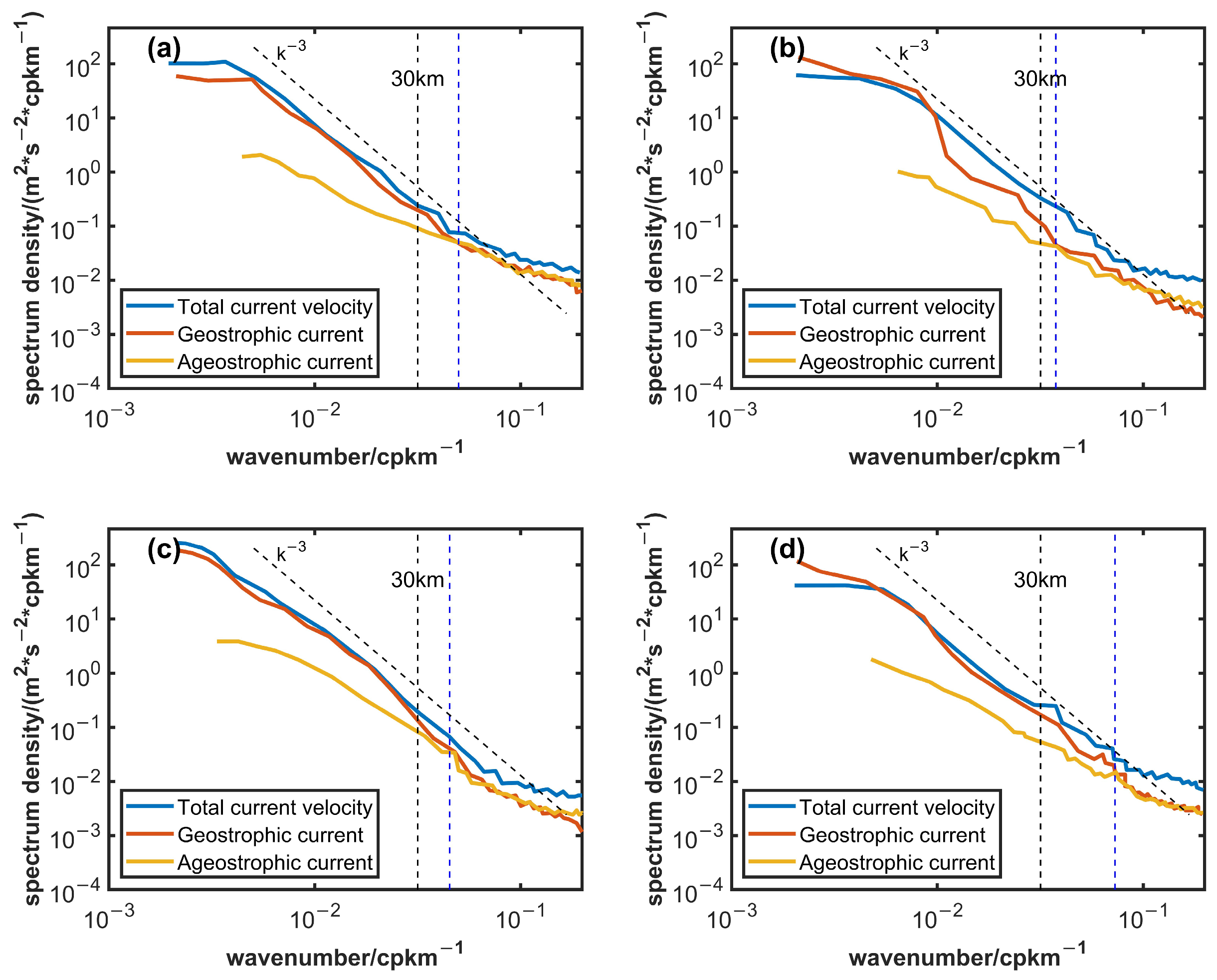
3.4. Distribution of Kinetic Energy Spectrum in the Kuroshio

The calculation results of wave number spectrum at a horizontal scale smaller than 10 km are greatly affected by the resolution of the observation data [16]. To ensure the reliability of the analysis, only results pertaining to horizontal scales larger than 10 km are discussed. The first baroclinic Rossby deformation radius of the Kuroshio is approximately 30 to 40 km, thereby defining the 10 to 30 km range as the submesoscale region for this study [15].

In the strong current region (Figure 6), the kinetic energy spectrum of the ageostrophic component is significantly smaller than that of the geostrophic component. The slope of the total kinetic energy spectrum remains around −3 and slightly exceeds −3 in the mesoscale range above 30 km. Additionally, the transition scale in summer and autumn is marginally larger than in spring and winter, generally remaining within the 10–30 km range. While the kinetic energy spectrum density of ageostrophic flow at the mesoscale is low, its activity on a smaller scale varies notably with the seasons, particularly in periods of strong wind fields and enhanced ocean mixing, such as spring and winter, where the contribution of ageostrophic effects is more substantial [50].

The slope of the total kinetic energy spectrum in the slow current area is approximately −3 for horizontal scales ranging from 30 to 200 km (Figure 7). The seasonal variation in the transition scale is significant, with summer (~28 km) much larger than winter (~13 km). In summer, the total kinetic energy spectrum generally follows a slope of −3 for wavelengths greater than the transition scale. Moreover, the kinetic energy in the slow current area for scales smaller than 30 km is notably higher in spring and winter compared to summer and autumn. The baroclinic instability of the mixed layer effectively stimulates submesoscale motion, and the deeper the mixed layer, the more effective the release of potential energy from front instability caused by secondary circulation [47,48]. The buoyancy anomalies and geostrophic flow along the front lead to a pattern where lighter fluid rises and heavier fluid sinks, enhancing vertical stratification and converting potential energy into kinetic energy, thus enhancing the contribution of ageostrophic motion to the total kinetic energy in spring and winter.

In summary, the kinetic energy across the mesoscale range (30–200 km) remains relatively stable throughout the four seasons. Within the submesoscale range (10–30 km), kinetic energy is higher in spring and winter than in summer and autumn, highlighting the significant impact of seasonal variations on kinetic energy at this scale. The observed seasonal differences in the transition scale between the strong and slow current areas of the Kuroshio suggest that the transition scale may be influenced by the instability of the mixed layer [16]. During spring and winter, stratification is typically weak, and surface layer density increases due to cooler temperatures, leading to more vigorous vertical mixing. Consequently, the transition scale is smaller in these seasons compared to summer and autumn.

3.5. Distribution of Kinetic Energy Transfer Rate in the Kuroshio

Figure 8 examines the spatio-temporal distribution of the kinetic energy transfer rate (HSP, VSP, and BC) in the Kuroshio. During summer (Figure 8a), particularly in the strong current area near the coast of Japan where the main axis of the Kuroshio is located, HSP demonstrates a significant positive value, indicating kinetic energy generation through horizontal shear, transferring energy from geostrophic flow to submesoscale flows. East of the Kuroshio’s main axis and in areas with slower currents, HSP values exhibit an alternating pattern of positive and negative values. In winter (Figure 8b), the distribution of HSP within the Kuroshio becomes more dispersed, suggesting a more complex kinetic energy transfer process. Although ocean stratification is reduced in winter compared to summer, horizontal energy transfer intensifies due to increased vertical mixing, particularly in the strong current region.

The distribution pattern of VSP (Figure 8c,d) is similar that of HSP, with the negative regions predominantly located in the strong current area near the coast of Japan along the main axis of the Kuroshio. This indicates that kinetic energy is being dissipated or reduced through vertical shear, transferring energy from submesoscale flow to mesoscale flow. Additionally, in the eastern region of the main Kuroshio axis and in areas with slower currents, VSP values show an alternating pattern of positive and negative values.

And the BC has strong positive values in the Kuroshio (Figure 8e,f), whose magnitude is much larger than the VSP and HSP in the same regions. This indicates that submesoscales predominantly obtain their KE through the release of APE. Although BC is greater than HSP and VSP, their magnitudes are comparable. The horizontal and vertical shear instability of the background currents during their interactions with the topography is also significant and cannot be ignored.

Figure 9 presents the time series of changes in horizontal shear production (HSP), vertical shear production (VSP), and baroclinic instability (BC) in the Kuroshio’s strong and slow current areas. In the strong current area, HSP and BC remain positive throughout the year, while VSP consistently shows negative values. The results indicate that seasonal variations of HSP and VSP are not significant in both winter and summer seasons. However, BC is much stronger in winter, with average values of HSP at 5.0 × 10⁻⁶ m² s⁻³, VSP at −4.2 × 10⁻⁶ m² s⁻³, and BC at 10.9 × 10⁻⁶ m² s⁻³. Notably, BC is significantly greater than both HSP and VSP. In contrast, in the slow current area, HSP and VSP, though smaller than in the strong current area, display significant fluctuations over the year, with BC also showing higher values in winter. The average values are 1.6 × 10⁻⁷ m² s⁻³ for HSP, −3.5 × 10⁻⁷ m² s⁻³ for VSP, and 7.8 × 10⁻⁷ m² s⁻³ for BC. From the averages of HSP and VSP in Figure 9a and b, we observe that although there is an alternation between positive and negative values, HSP typically exceeds VSP in the strong current area. This suggests that mesoscales tend to transfer part of their kinetic energy to submesoscale eddies. Conversely, in the slow current area, VSP typically exceeds HSP, suggesting that submesoscale motions transfer part of their KE inversely to mesoscale motions. In general, submesoscales obtain their KE through BC and HSP while losing a small portion of their KE through VSP in the Kuroshio area.

4. Conclusions

Submesoscale ageostrophic energy is larger in winter and spring than in summer and autumn, while geostrophic energy peaks during summer and autumn. There is a significant correlation between geostrophic strain, mixed layer depth, and ageostrophic energy. Notably, enhancements in geostrophic strain and changes in mixed layer depth greatly influence submesoscale ageostrophic energy, particularly in areas of strong current. With the submesoscale kinetic energy being particularly sensitive to seasonal variation, the transition scale of kinetic energy in summer and autumn is generally larger compared to those in spring and winter. Furthermore, the transition scale of kinetic energy during summer and autumn is typically larger than in spring and winter. The HSP remains positive and VSP negative throughout the year in the strong current area, with HSP generally exceeding VSP, kinetic energy cascades forward from geostrophic motion to ageostrophic motion through horizontal shear. In contrast, changes in HSP and VSP in the slow current area are more complex, with VSP generally greater than HSP, the kinetic energy inverse cascades forward from ageostrophic motion to geostrophic motion through vertical shear. The BC is greater than the VSP and HSP in the Kuroshio regions. Submesoscale ageostrophic motion predominantly obtains its kinetic energy through the release of available potential energy (APE). Submesoscale ageostrophic motion also gains KE through baroclinic instability (BC) and horizontal shear production (HSP) while losing a small portion of its KE through vertical shear production (VSP) in the Kuroshio area.

References

1. Chunhua, Q.; Zihao, Y.; Dongxiao, W.; Ming, F.; Jingzhi, S. The Enhancement of Submesoscale Ageostrophic Motion on the Mesoscale Eddies in the South China Sea. J. Geophys. Res. Ocean. 2022, 127, e2022JC018736. [Google Scholar] [CrossRef]
2. McWilliams, J.C. Submesoscale surface fronts and filaments: Secondary circulation, buoyancy flux, and frontogenesis. J. Fluid Mech. 2017, 823, 391–432. [Google Scholar] [CrossRef]
3. D’asaro, E.; Lee, C.; Rainville, L.; Harcourt, R.; Thomas, L. Enhanced turbulence and energy dissipation at ocean fronts. Science 2011, 332, 318–322. [Google Scholar] [CrossRef] [PubMed]
4. Flagg, C.N.; Dunn, M.; Wang, D.P.; Rossby, H.T.; Benway, R.L. A study of the currents of the outer shelf and upper slope from a decade of shipboard ADCP observations in the Middle Atlantic Bight. J. Geophys. Res. Ocean. 2006, 111. [Google Scholar] [CrossRef]
5. Nagai, T.; Tandon, A.; Rudnick, D.L. Two-dimensional ageostrophic secondary circulation at ocean fronts due to vertical mixing and large-scale deformation. J. Geophys. Res. Ocean. 2006, 111. [Google Scholar] [CrossRef]
6. Zhang, Z.; Qiu, B.; Klein, P.; Travis, S. The influence of geostrophic strain on oceanic ageostrophic motion and surface chlorophyll. Nat. Commun. 2019, 10, 2838. [Google Scholar] [CrossRef] [PubMed]
7. Qiu, B.; Kelly, K.A.; Joyce, T.M. Mean flow and variability in the Kuroshio Extension from Geosat altimetry data. J. Geophys. Res. Ocean. 1991, 96, 18491–18507. [Google Scholar] [CrossRef]
8. Cao, H.; Fox-Kemper, B.; Jing, Z. Submesoscale eddies in the upper ocean of the Kuroshio Extension from high-resolution simulation: Energy budget. J. Phys. Oceanogr. 2021, 51, 2181–2201. [Google Scholar] [CrossRef]
9. Morrow, R.; Fu, L.-L. Observing mesoscale to submesoscale dynamics today, and in the future with SWOT. In Proceedings of the 2011 IEEE International Geoscience and Remote Sensing Symposium, Vancouver, BC, Canada, 24–29 July 2011; pp. 2689–2691. [Google Scholar] [CrossRef]
10. Nagai, T.; Tandon, A.; Gruber, N.; McWilliams, J.C. Biological and physical impacts of ageostrophic frontal circulations driven by confluent flow and vertical mixing. Dyn. Atmos. Ocean. 2008, 45, 229–251. [Google Scholar] [CrossRef]
11. Zhang, Z.; Zhao, W.; Qiu, B.; Tian, J. Anticyclonic eddy sheddings from Kuroshio loop and the accompanying cyclonic eddy in the northeastern South China Sea. J. Phys. Oceanogr. 2017, 47, 1243–1259. [Google Scholar] [CrossRef]
12. Hoskins, B.J.; Bretherton, F.P. Atmospheric frontogenesis models: Mathematical formulation and solution. J. Atmos. Sci. 1972, 29, 11–37. [Google Scholar] [CrossRef]
13. Qiu, B.; Nakano, T.; Chen, S.; Klein, P. Bi-directional energy cascades in the Pacific Ocean from equator to subarctic gyre. Geophys. Res. Lett. 2022, 49, e2022GL097713. [Google Scholar] [CrossRef]
14. Siegelman, L.; Klein, P.; Rivière, P.; Thompson, A.F.; Torres, H.S.; Flexas, M.; Menemenlis, D. Enhanced upward heat transport at deep submesoscale ocean fronts. Nat. Geosci. 2020, 13, 50–55. [Google Scholar] [CrossRef]
15. Zhang, Y.; Zhang, S.; Afanasyev, Y.D. Energy cascades in surface semi-geostrophic turbulence. Authorea Prepr. 2024. [Google Scholar] [CrossRef]
16. Lin, R.Q.; Chubb, S. Energy cascades in the upper ocean. Chin. J. Oceanol. Limnol. 2006, 24, 225–235. [Google Scholar] [CrossRef]
17. Sasaki, H.; Klein, P.; Qiu, B.; Sasai, Y. Impact of oceanic-scale interactions on the seasonal modulation of ocean dynamics by the atmosphere. Nat. Commun. 2014, 5, 5636. [Google Scholar] [CrossRef]
18. Bos, W.; Kadoch, B.; Schneider, K.; Bertoglio, J. Inertial range scaling of the scalar flux spectrum in two-dimensional turbulence. Phys. Fluids 2009, 21, 115105:115101–115105:115108. [Google Scholar] [CrossRef]
19. Colas, F.; Capet, X.; McWilliams, J.C.; Li, Z. Mesoscale eddy buoyancy flux and eddy-induced circulation in Eastern Boundary Currents. J. Phys. Oceanogr. 2013, 43, 1073–1095. [Google Scholar] [CrossRef]
20. Li, S.; Zhong, Y.; Zhou, M.; Wu, H.; Gao, Y.; Zhou, P.; Wang, Y.; Zhang, Z.; Zhang, H. The Summer Kuroshio Intrusion Into the East China Sea Revealed by a New Mixed-Layer Water Mass Analysis. J. Geophys. Res. Ocean. 2024, 129, e2023JC020827. [Google Scholar] [CrossRef]
21. Jiang, Y.X.; Sun, J.X.; Wu, X.H.; Wang, H. Impacts of the Kuroshio Extension Stability on the Storm-track over the North Pacific. J. Phys. Conf. Ser. 2024, 2718, 012039. [Google Scholar] [CrossRef]
22. Qiu, B.; Scott, R.B.; Chen, S. Length scales of eddy generation and nonlinear evolution of the seasonally modulated South Pacific Subtropical Countercurrent. J. Phys. Oceanogr. 2008, 38, 1515–1528. [Google Scholar] [CrossRef]
23. Zhang, Z.; Qiu, B. Evolution of submesoscale ageostrophic motions through the life cycle of oceanic mesoscale eddies. Geophys. Res. Lett. 2018, 45, 11847–11855. [Google Scholar] [CrossRef]
24. Kuo, Y.-C.; Tseng, Y.-H. Influence of anomalous low-level circulation on the Kuroshio in the Luzon Strait during ENSO. Ocean Model. 2021, 159, 101759. [Google Scholar] [CrossRef]
25. Yang, P.; Jing, Z.; Sun, B.; Wu, L.; Qiu, B.; Chang, P.; Ramachandran, S.; Yuan, C. On the Upper-Ocean Vertical Eddy Heat Transport in the Kuroshio Extension. Part II: Effects of Air–Sea Interactions. J. Phys. Oceanogr. 2021, 51, 3297–3312. [Google Scholar] [CrossRef]
26. Motomura, H.; Matsunuma, M. Fish diversity along the Kuroshio Current. In Fish Diversity of Japan: Evolution, Zoogeography, and Conservation; Springer: Berlin/Heidelberg, Germany, 2022; pp. 63–78. [Google Scholar] [CrossRef]
27. Tozuka, T.; Sasai, Y.; Yasunaka, S.; Sasaki, H.; Nonaka, M. Simulated decadal variations of surface and subsurface phytoplankton in the upstream Kuroshio Extension region. Prog. Earth Planet. Sci. 2022, 9, 70. [Google Scholar] [CrossRef]
28. Masaaki, S.; Yohei, N.; Masakazu, H. Potential stocks of reef fish-based ecosystem services in the Kuroshio Current region: Their relationship with latitude and biodiversity. Popul. Ecol. 2020, 63, 75–91. [Google Scholar] [CrossRef]
29. Shuyang, M.; Yongjun, T.; Jianchao, L.; Peilong, J.; Peng, S.; Zhenjiang, Y.; Yang, L.; Yoshiro, W. Incorporating thermal niche to benefit understanding climate-induced biological variability in small pelagic fishes in the Kuroshio ecosystem. Fish. Oceanogr. 2022, 31, 172–190. [Google Scholar] [CrossRef]
30. Li, Q.P.; Wang, Y.; Dong, Y.; Gan, J. Modeling long-term change of planktonic ecosystems in the northern S outh C hina S ea and the upstream K uroshio C urrent. J. Geophys. Res. Ocean 2015, 120, 3913–3936. [Google Scholar] [CrossRef]
31. Yatsu, A.; Chiba, S.; Yamanaka, Y.; Ito, S.I.; Shimizu, Y.; Kaeriyama, M.; Watanabe, Y. Climate forcing and the Kuroshio/Oyashio ecosystem. ICES J. Mar. Sci. 2013, 70, 922–933. [Google Scholar] [CrossRef]
32. Chiba, S.; Lorenzo, E.D.; Davis, A.; Keister, J.E.; Taguchi, B.; Sasai, Y.; Sugisaki, H. Large-scale climate control of zooplankton transport and biogeography in the Kuroshio-Oyashio Extension region. Geophys. Res. Lett. 2013, 40, 5182–5187. [Google Scholar] [CrossRef]
33. Zhang, J.; Li, C.; Luo, X. Response of Sea Surface Heat Flux to the Kuroshio Extension Ocean Front for Different Background Wind Fields. J. Coast. Res. 2020, 99, 332–339. [Google Scholar] [CrossRef]
34. Shan, X.; Jing, Z.; Gan, B.; Wu, L.; Chang, P.; Ma, X.; Wang, S.; Chen, Z.; Yang, H. Surface Heat Flux Induced by Mesoscale Eddies Cools the Kuroshio-Oyashio Extension Region. Geophys. Res. Lett. 2020, 47, e2019GL086050. [Google Scholar] [CrossRef]
35. Tozuka, T.; Cronin, M.F.; Tomita, H. Surface frontogenesis by surface heat fluxes in the upstream Kuroshio Extension region. Sci. Rep. 2017, 7, 10258. [Google Scholar] [CrossRef]
36. Taguchi, B.; Qiu, B.; Nonaka, M.; Sasaki, H.; Xie, S.-P.; Schneider, N. Decadal variability of the Kuroshio Extension: Mesoscale eddies and recirculations. Ocean Dyn. 2010, 60, 673–691. [Google Scholar] [CrossRef]
37. Chang, Y.L.K.; Miyazawa, Y.; Miller, M.J.; Tsukamoto, K. Influence of ocean circulation and the Kuroshio large meander on the 2018 Japanese eel recruitment season. PLoS ONE 2019, 14, e0223262. [Google Scholar] [CrossRef] [PubMed]
38. Chen, L.; Jia, Y.; Liu, Q. Oceanic eddy-driven atmospheric secondary circulation in the winter Kuroshio Extension region. J. Oceanogr. 2017, 73, 295–307. [Google Scholar] [CrossRef]
39. Qiu, B.; Chen, S. Variability of the Kuroshio Extension jet, recirculation gyre, and mesoscale eddies on decadal time scales. J. Phys. Oceanogr. 2005, 35, 2090–2103. [Google Scholar] [CrossRef]
40. Joh, Y.; Delworth, T.L.; Wittenberg, A.T.; Cooke, W.F.; Rosati, A.J.; Zhang, L. Stronger decadal variability of the Kuroshio Extension under simulated future climate change. NPJ Clim. Atmos. Sci. 2022, 5, 63. [Google Scholar] [CrossRef]
41. Geng, Y.; Ren, H.-L.; Ma, X.; Zhao, S.; Nie, Y. Responses of East Asian Climate to SST Anomalies in the Kuroshio Extension Region during Boreal Autumn. J. Clim. 2022, 35, 7007–7023. [Google Scholar] [CrossRef]
42. Ji, J.; Dong, C.; Zhang, B.; Liu, Y.; Zou, B.; King, G.P.; Xu, G.; Chen, D. Oceanic eddy characteristics and generation mechanisms in the Kuroshio Extension region. J. Geophys. Res. Ocean. 2018, 123, 8548–8567. [Google Scholar] [CrossRef]
43. Zhang, Z.; Xie, L.; Zheng, Q.; Li, M.; Li, J.; Li, M. Coherence of Eddy Kinetic Energy Variation during Eddy Life Span to Low-Frequency Ageostrophic Energy. Remote Sens. 2022, 14, 3793. [Google Scholar] [CrossRef]
44. Zhang, J.; Zhang, Z.; Qiu, B.; Zhang, X.; Sasaki, H.; Zhao, W.; Tian, J. Seasonal modulation of submesoscale kinetic energy in the upper ocean of the northeastern South China Sea. J. Geophys. Res. Ocean. 2021, 126, e2021JC017695. [Google Scholar] [CrossRef]
45. Gula, J.; Molemaker, M.J.; McWilliams, J.C. Topographic vorticity generation, submesoscale instability and vortex street formation in the Gulf Stream. Geophys. Res. Lett. 2015, 42, 4054–4062. [Google Scholar] [CrossRef]
46. Srinivasan, K.; McWilliams, J.C.; Renault, L.; Hristova, H.G.; Molemaker, J.; Kessler, W.S. Topographic and mixed layer submesoscale currents in the near-surface southwestern tropical Pacific. J. Phys. Oceanogr. 2017, 47, 1221–1242. [Google Scholar] [CrossRef]
47. Boccaletti, G.; Ferrari, R.; Fox-Kemper, B. Mixed layer instabilities and restratification. J. Phys. Oceanogr. 2007, 37, 2228–2250. [Google Scholar] [CrossRef]
48. Fox-Kemper, B.; Ferrari, R.; Hallberg, R. Parameterization of mixed layer eddies. Part I: Theory and diagnosis. J. Phys. Oceanogr. 2008, 38, 1145–1165. [Google Scholar] [CrossRef]
49. Schubert, R.; Vergara, O.; Gula, J. The open ocean kinetic energy cascade is strongest in late winter and spring. Commun. Earth Environ. 2023, 4, 450. [Google Scholar] [CrossRef]
50. Evans, D.G.; Frajka-Williams, E.; Naveira Garabato, A.C. Dissipation of mesoscale eddies at a western boundary via a direct energy cascade. Sci. Rep. 2022, 12, 887. [Google Scholar] [CrossRef]
Figure 1. The multi-year average distribution of EKE (eddy kinetic energy of the mesoscale eddies) in the Kuroshio region (20–60° N, 120–180° E).
Jmse 12 01121 g001
Figure 2. Ocean surface geostrophic kinetic energy (a,b), submesoscale ageostrophic kinetic energy (c,d), and geostrophic strain (e,f) during summer and autumn (a,c,e) and winter and spring (b,d,f).
Jmse 12 01121 g002
Figure 4. Vertical changes in submesoscale KE under four different conditions in strong current area (a) and slow current area (b). Weak MSR with shallow MLD, strong MSR with shallow MLD, weak MSR with deep MLD, and strong MSR with deep MLD are represented by blue, red, yellow, and purple lines, respectively.
Jmse 12 01121 g004
Figure 5. Correlation between MLD (a,c), MSR (b,d), and average submesoscale KE above 150 m in the strong current area (a,b) and slow current area (c,d).
Jmse 12 01121 g005aJmse 12 01121 g005b
Figure 6. Kuroshio strong current area ((a) spring, (b) summer, (c) autumn, (d) winter), the blue line represents the total current velocity kinetic energy spectrum density, the red line represents the geostrophic kinetic energy spectrum density, the yellow line represents the submesoscale ageostrophic kinetic energy spectrum density line, the black dotted line represents the 30 km scale position, and the blue dotted line represents the transition scale position of geostrophic current and submesoscale ageostrophic current.
Jmse 12 01121 g006
Figure 7. Kuroshio slow current area ((a) spring, (b) summer, (c) autumn, (d) winter), the blue line represents the total current velocity kinetic energy spectrum density, the red line represents the geostrophic kinetic energy spectrum density, the yellow line represents the submesoscale ageostrophic energy spectrum density line, the black dotted line represents the 30 km scale position, and the blue dotted line represents the transition scale position of geostrophic currents and submesoscale ageostrophic currents.
Jmse 12 01121 g007
Figure 8. Spatial distribution of horizontal shear production (summer (a), winter, (b)), vertical shear production (summer (c), winter (d)), and baroclinic instability (summer (e), winter (f)) of geostrophic and submesoscale ageostrophic motions.
Jmse 12 01121 g008
Figure 9. Time series of horizontal shear production, vertical shear production, and BC in the Kuroshio strong current area (a) and slow current area (b). The blue line represents the BC, the black line represents the HSP, the red line represents the VSP, and the dotted line represents the average value.
Jmse 12 01121 g009
Disclaimer/Publisher’s Note: The statements, opinions and data contained in all publications are solely those of the individual author(s) and contributor(s) and not of MDPI and/or the editor(s). MDPI and/or the editor(s) disclaim responsibility for any injury to people or property resulting from any ideas, methods, instructions or products referred to in the content.