Article

A Wind Power Combination Forecasting Method Based on GASF Image Representation and UniFormer

1
School of Naval Architecture, Ocean and Energy Power Engineering, Wuhan University of Technology, Wuhan 430063, China
2
State Key Laboratory of Maritime Technology and Safety, Wuhan University of Technology, Wuhan 430063, China
*
Author to whom correspondence should be addressed.
J. Mar. Sci. Eng. 2024, 12(7), 1173; https://doi.org/10.3390/jmse12071173
Submission received: 28 May 2024 / Revised: 28 June 2024 / Accepted: 10 July 2024 / Published: 13 July 2024

Abstract

:
In the field of wind power prediction, traditional methods typically rely on one-dimensional time-series data for feature extraction and prediction. In this study, we propose an innovative short-term wind power forecasting approach using a “visual” 2D image prediction method that effectively utilizes spatial pattern information in time-series data by combining wind power series and related environmental features into a 2D GASF image. Firstly, the wind power data are decomposed using the ICEEMDAN algorithm optimized by the BWO (Beluga Whale Optimization) algorithm, extracting the submodal IMF (Intrinsic Mode Function) components with different frequencies. Then, modal reconstruction is performed on the basis of the permutation entropy value of the IMF components, selecting meteorological features highly correlated with reconstructed components through Spearman correlation analysis for data splicing and superposition before converting them into GASF images. Finally, the GASF images are input into the UniFormer model for wind power sequence prediction. By leveraging wind power data predictions from a coastal wind farm in East China and Sotavento in Spain, this study demonstrates the significant benefits and potential applications of this methodology for precise wind power forecasting. This research combines the advantages of image feature extraction and time-series prediction to offer novel perspectives and tools for predicting renewable energy sources such as wind power.

1. Introduction

With the continuous advancement in renewable energy and the optimization of power infrastructure, wind power has emerged as a pivotal element in the global transition toward sustainable energy [1]. However, wind power is susceptible to meteorological factors such as wind speed and direction, presenting significant challenges for efficient grid integration and energy scheduling due to its intermittent nature and variability [2]. Accurate short-term forecasting of wind power is imperative for mitigating these challenges, effectively managing energy resources, and enhancing grid stability. Despite the multidimensional features present in wind power and meteorological sensor data, conventional time-series forecasting methods often treat these features as independent one-dimensional sequences to extract dominant characteristics, such as the mean, variance, and skewness. This approach fails to deeply mine the relationships among the data, thereby limiting its ability to handle the complex, nonlinear, and nonstationary nature of wind power dynamics [3]. Moreover, it may not fully exploit potential correlations between wind power generation and related environmental variables (e.g., wind speed, temperature, and atmospheric pressure). Consequently, their prediction accuracy is frequently constrained by the inherent limitations of representing one-dimensional data and employing models.
To tackle these challenges, this study introduces an innovative approach named BIGU (BWO-ICEEMDAN-GASF-UniFormer), which combines the benefits of image-based analysis and advanced deep learning techniques. It integrates multiple stages of data processing and feature selection to enhance the predictive performance of wind power forecasting. By transforming wind power time series and associated environmental features into two-dimensional images, such as GASFs (Gramian Angular Summation Fields), the problem shifts from traditional one-dimensional time-series analysis to a “visual” pattern recognition task. This approach encodes multidimensional information, including phase information, periodic features, and local changes in the time series, as spatial features in the image. Consequently, it enables the visualization of more intricate patterns in a two-dimensional space and enhances the model’s capacity to effectively recognize and extract these complex multiscale features. This transformation facilitates capturing both the spatial patterns and temporal dependencies present in the data.
By integrating the benefits of image-based feature extraction and time-series prediction, our research endeavors to bridge the gap between conventional forecasting methods and emerging requirements in the renewable energy sector, thereby offering novel insights and tools for efficient energy management.

1.1. Literature Survey

The current methods for wind power prediction can be broadly categorized into the following three groups: physical models, statistical approaches, and artificial intelligence techniques [4]. Among these, the establishment process of a physical model is more intricate and requires extensive calculations to predict wind power through functional relationship modeling, making it impractical for wind power prediction [5]. Statistical methods employ learning algorithms to identify patterns in features by combining power data with weather data to forecast future wind power. However, statistical methods rely on the smoothness of the time series and have limited capacity to fit complex curves [6]. Traditional statistical approaches struggle with extracting mapping relationships due to the high randomness and volatility inherent in wind power sequences, resulting in challenges achieving the desired prediction accuracy.
Artificial intelligence methods utilize a substantial amount of historical wind power data to train neural network models, enabling them to effectively capture the temporal trends in time-series modeling compared to previous approaches such as Support Vector Machines [7], Artificial Neural Networks [8], and deep learning algorithms. Deep learning models, specifically Convolutional Neural Networks (CNNs) and Long Short-Term Memory (LSTM), are increasingly employed in wind power prediction research. However, because of the multifaceted nature of wind power generation influenced by various factors, individual neural network prediction models often struggle to fully capture sequential features. To address this limitation, combined prediction methods leverage the strengths of each model or method for enhanced accuracy. In a recent study [9], the MIC-PBT DWTimesNet model was proposed for the multistep prediction of wind power generation. By replacing the original convolutional structure with dilated convolution and Weight Normalization (WN), the prediction error of the TimesNet model can be improved. Additionally, a Population-Based Training (PBT) algorithm was introduced to optimize the model, while feature selection using the Maximal Information Coefficient (MIC) method effectively reduced the computational workload and improved the prediction accuracy. Another study [10] combined a Graph Convolutional Neural Network (GCN) with a Gated Recurrent Unit (GRU) to predict simulated and actual wind speeds, as well as wind power datasets. The long-term prediction results demonstrate the performance capabilities of the GCN. In the literature [11], a dual-layer Shared Weight Long Short-Term Memory Network (SWLSTM) prediction model based on streaming learning is proposed, which incorporates the influence of meteorological environmental factors, wind turbine parameters, historical wind power, and prediction errors. This model constructs a two-layer SWLSTM prediction framework.
Another study [12] employed machine learning techniques to develop wind speed prediction models and introduced a real-time evaluation method for wind power generation using LSTM, GRUs, superimposed RNNs, and LSTM unit neural networks. The wind speed prediction models were categorized into yearly and seasonal modes based on seasonal characteristics to forecast wind speeds for the next 1 to 12 h and evaluate their performance. In the study in [13], the MTTFA (Multi-Task Temporal Feature Attention)-LSTM model was proposed for multivariate/multistep wind power prediction based on historical power and meteorological data. It incorporates task-sharing layers and task-specifying layers to facilitate cofeature extraction and discriminate task-specific features, respectively. Furthermore, an attention mechanism was employed to dynamically adjust the weights of the temporal features. The simulation results demonstrate that the proposed model effectively captures the intricate nonlinear interdependencies among multidimensional data. In the absence of sufficient historical data, this study [14] proposes a novel prediction model that combines Secondary Evolutionary Generative Adversarial Networks (SEGANs) and a Dual-Dimension Attention Mechanism (DDAM) with a Bidirectional Gated Recurrent Unit (BiGRU), aiming to address the issue of few-shot learning in wind power prediction for new wind farms. The experimental results demonstrate a promising performance in short-term prediction for newly established wind farms.
The application of deep learning methods has significantly enhanced the accuracy of wind power prediction; however, the output of wind turbines is influenced by multiple factors characterized by strong nonlinearity and instability. Signal decomposition techniques can effectively decompose the original signal into Intrinsic Mode Functions (IMFs), thereby revealing its multiscale laws. The decomposed signal exhibits smoother characteristics, enabling neural networks to better capture its dynamic variations. Moreover, through prediction and superposition reconstruction of subsequence components, the combined prediction method based on signal decomposition can effectively improve the accuracy of wind power forecasting. This approach is widely employed in current research endeavors. A novel approach for wind speed prediction based on its characteristics was proposed in a recent study [15]. Initially, the wind speed was decomposed into three components—nonlinear, linear, and noise parts—using VMD (Variational Modal Decomposition). These components were then combined to construct a VMD-PRBF-ARMA-E model for offline deterministic and uncertainty predictions, which demonstrated the superiority of this model. Another study [16] introduced a soft sensor model based on an LSTM network and highlighted the improved prediction accuracy achieved by combining an LSTM network with the VMD method. Reference [17] proposed an integrated prediction model that combines LSTM, EEMD (Ensemble Empirical Mode Decomposition), and PSO (Particle Swarm Optimization). EEMD is utilized to mitigate the impact of nonsmoothness in sequences on prediction accuracy, while PSO optimizes the hyperparameter values of the LSTM. The final prediction results were obtained by aggregating the predicted values from each subsequence. In the study in [18], data were decomposed twice using OVMD-ICEEMDAN-PE, and a prediction model for each component was constructed on the basis of the decomposed data. Improved state transition algorithms were introduced to optimize the CNN-BiLSTM (Bidirectional Long Short-Term Memory), Temporal Convolutional Network (TCN), and GRU hyperparameters. Linear weights were combined with optimal hyperparameters solved for each model to achieve accurate predictions.
The majority of the aforementioned studies employed conventional forecasting methods that rely on one-dimensional time-series data. Currently, there is limited research investigating the integration of computer vision with time-series analysis, particularly within the domain of wind power forecasting. Reference [3] introduces an innovative “Image-feature-stacking prediction model” for univariate time-series data prediction by converting it into corresponding images and utilizing an optimized Inception-v1 network to extract hidden features from these images as input variables for predicting the daily PM2.5 concentration. In Reference [19], a combination of a Generative Adversarial Network (GAN) and an LSTM based on a Global Recurrence Plot (GRP) was proposed for forecasting rotary kiln temperatures. The use of a GRP transforms a one-dimensional time series into a two-dimensional image, enabling the exploitation of both global and local information within the time series. In the study in [20], time-series imaging techniques, including Gramian Angular Summation/Difference Field (GASF/GADF), Markov Transition Field (MTF), and Recurrent Plot (RP), were employed to encode the Standard Precipitation Evaporation Index (SPEI) sequences into images for feature extraction. The extracted features were then utilized in conjunction with imaging datasets and CNNs to train a feature extraction network. Subsequently, four regression models, namely, Random Forest (RF), LSTM, Wavelet Neural Network (WNN), and Support Vector Regression (SVR), were employed for modeling and drought prediction.

1.2. Main Contributions

This paper presents a novel approach for short-term wind power prediction based on deep learning, incorporating signal decomposition and image processing techniques. The key contributions of this study are as follows:
(1)
Introducing the BIGU framework, which combines ICEEMDAN, optimized by the BWO algorithm, for signal decomposition and GASF for transforming time-series data into 2D images to capture intricate temporal patterns and spatial relationships, thereby enhancing the feature set for UniFormer models used in accurate wind power prediction.
(2)
Employing permutation entropy to reconstruct the IMF into high-frequency, low-frequency, and trend components, followed by Spearman correlation analysis for feature selection to intelligently integrate meteorological variables. This process ensures that the most relevant features are incorporated into the GASF image, enriching the input data for predictive modeling.
(3)
The efficacy of the BIGU method is substantiated through diverse case studies, emphasizing its practical advantages and potential applications.

1.3. Organization of the Paper

The subsequent sections of the paper are organized as follows: Section 2 provides an overview of the relevant methodologies and model principles employed in this study. Section 3 presents the structure of the predictive model and evaluation metrics used. Section 4 and Section 5 demonstrate the effectiveness of the proposed approach through two case tests. Finally, Section 6 offers a comprehensive conclusion along with future suggestions.

2. Research Methods

2.1. BWO-ICEEMDAN

2.1.1. ICEEMDAN Decomposition Principle

Because of the intermittent nature of the original signal, the classical Empirical Mode Decomposition (EMD) algorithm suffers from modal aliasing. The EEMD algorithm addresses this issue by introducing Gaussian white noise to eliminate signal intermittency. However, this approach introduces difficult-to-eliminate white noise and increases reconstruction errors. To overcome these limitations, the Complete Ensemble EMD with Adaptive Noise (CEEMDAN) algorithm adds positively and negatively complementary white noise at each stage of modal decomposition to eliminate residual interference caused by white noise. Nevertheless, pseudo-modal components still pose a challenge in CEEMDAN. In order to further mitigate interference and aliasing resulting from adding white noise during EMD decomposition, the ICEEMDAN algorithm has been proposed. ICEEMDAN eliminates such issues by incorporating modal components obtained from decomposing the added white noise using EMD. The decomposition steps of ICEEMDAN are as follows [21]:
(1)
Incorporate i sets of modal components of white noise into the original signal sequence, x , to generate the noise-added signal sequence, X 1 ( i ) , as follows:
X 1 ( i ) = x + B 1 E 1 w i .
The k th signal-to-noise ratio is denoted as B k , the white noise signal is represented by w ( i ) , and E k ( ) refers to the k th modal component of the EMD decomposition.
(2)
Use EMD to perform N repeated decompositions on the additive noise signal, subtract it from the noisy signal, and calculate the average value to obtain the first residual signal, R 1 , and its corresponding intrinsic mode function, I m f 1 , as follows:
  R 1 = X 1 ( i ) E 1 ( X 1 ( i ) ) ,
  I m f 1 = x R 1 ,
where ⟨ ⟩ denotes the process of averaging.
(3)
Incorporate multiple white noise components into R 1 , followed by calculating the mean to obtain X 2 ( i ) = R 1 + B 2 E 2 ( w ( i ) ) . Then, perform a subtraction operation with R 1 to derive the second modal component, I m f 2 , as follows:
R 2 = X 2 i E 2 X 2 i ,
  I m f 2 = R 1 R 2 .
(4)
Repeat step (3) iteratively until the residual signal can no longer be decomposed and the decomposition termination condition is met, thereby obtaining all modal components.

2.1.2. BWO Algorithm

The decomposition effect of the ICEEMDAN method relies on the N s t d   (white noise amplitude weight) and N E (noise addition times). However, because of the strong nonlinearity and volatility exhibited by wind power sequences, empirically determined methods are highly stochastic and lack a theoretical foundation. Therefore, it is essential to select optimization methods applicable to wind power sequence prediction in order to guide the selection of decomposition parameters. Metaheuristic algorithms employ multiple candidate solutions that optimize each other, thereby avoiding local optimality and providing enhanced global search capabilities. Comparative studies have demonstrated that the BWO algorithm outperforms classical metaheuristic optimization algorithms in terms of both global search capability and efficient convergence.
The BWO algorithm, proposed by Zhong et al., in 2022 [22], draws inspiration from the behavioral patterns exhibited by beluga whales, including swimming, feeding, and whale falling. A schematic representation of the various stages of beluga whale behavior is depicted in Figure 1.
The theories outlining the stages of behavior are succinctly delineated below.
The beluga behavioral phase comprises the following three primary computational processes: exploration, exploitation, and whale fall. The positioning of the search agent during the exploration phase is determined by the synchronized swims of beluga whales. In the exploitation phase, a Levy flight strategy is introduced to enhance algorithm convergence, assuming that beluga whales employ this flight strategy for food capture. The whale fall phase simulates the behavior of a whale fall in each iteration, with subjective assumptions selecting probabilities for individual whale falls to simulate minor population changes. Adaptive whale fall probabilities and balance factors play a crucial role in controlling the exploration and exploitation capabilities within the algorithm. As the BWO algorithm operates via a population-based mechanism, beluga whales are considered search agents, whereby each one acts as a candidate solution continuously updated throughout optimization process. The position matrix model of the search agent is presented as follows:
X = x 1,1 x 1,2 x 1 , d x 2,1 x 2,2 x 2 , d x n , 1 x n , 2 x n , d ,
where n represents the population size of beluga whales, and d denotes the dimensionality of the design variable.
The fitness values for all belugas are stored accordingly:
F X = f ( x 1,1 , x 1,2 , , x 1 , d ) f ( x 2,1 , x 2,2 , , x 2 , d ) f ( x n , 1 , x n , 2 , , x n , d ) .
The BWO algorithm implements the transition of the population from exploration to exploitation based on the balance factor, B f , which is calculated as follows:
B f = B 0 × 1 t 2 T ,
where t represents the current iteration number, T denotes the total number of iterations, and B 0 is a randomly generated value ranging from 0 to 1 that varies with each iteration. A balance factor B f > 0.5 signifies the exploration phase, while B f 0.5 indicates the exploitation phase.

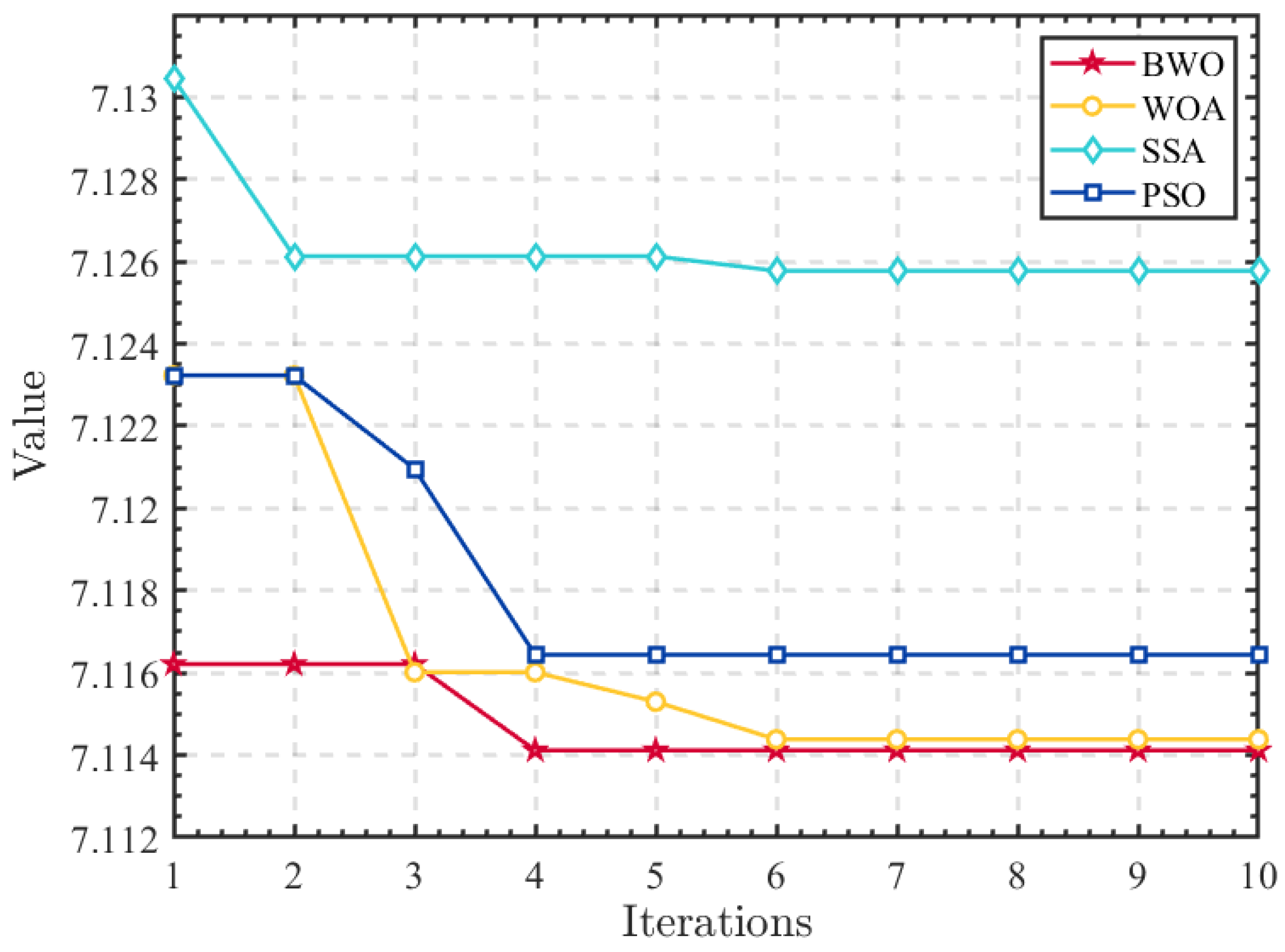
2.1.3. Parameter Optimization Process

The present study introduces an advanced swarm-based metaheuristic algorithm, namely, BWO, for optimizing the two parameters of ICEEMDAN using envelope entropy as the fitness function. Envelope entropy serves as a measure of sparsity in the original signal, whereby higher values indicate more noise and fewer informative features in the IMF, while lower values represent better decomposition.
For the IMF signal u with length m , the envelope entropy formula is as follows:
  E p = i = 1 m p i l o g 2 p i p i = a ( i ) / i = 1 m a ( i ) a ( i ) = u ( i ) 2 + H u ( i ) 2 ,
where E p is the envelope entropy of u , m is the length of u , p is the signal probability distribution, a is the envelope signal sequence obtained by the Hilbert demodulation of IMF signal u , and H · represents the Hilbert transform. The entropy value of the probability distribution sequence, p i , is referred to as envelope entropy, E P .
The optimization procedures are succinctly delineated below:
(1)
Initialize the population of the BWO algorithm; set the total number of iterations, T , and the population size, n ; and define the range of decision variables. Each individual consists of the following two decision variables: N s t d and N E . The initial solutions for n individuals are generated randomly.
(2)
Apply ICEEMDAN to decompose the wind power signal into its IMF components. Calculate the envelope entropy for each component and select the minimum value as the fitness function.
(3)
Determine whether the optimization has reached the termination condition of the algorithm. If it has, proceed to the next step; if not, update the population’s position based on the formula and parameters of the BWO algorithm and return to step (2).
(4)
Employ a greedy selection strategy based on fitness values to save the optimal combinations of ICEEMDAN parameters. Substitute these parameter values into the ICEEMDAN algorithm by replacing N s t d and N E with those from the best solution.
(5)
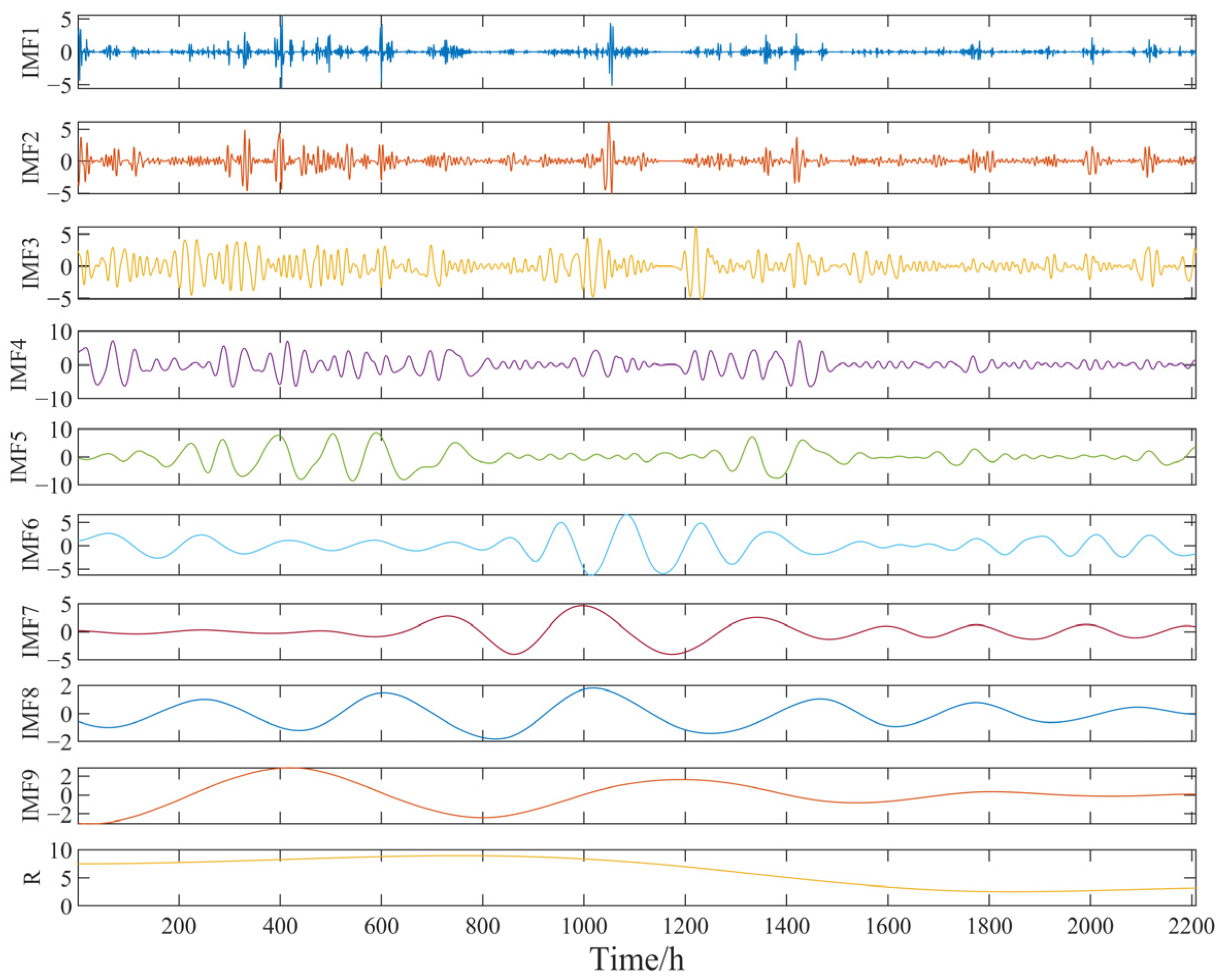
Use the optimized parameter combination to perform ICEEMDAN decomposition on the corresponding wind power sequence and obtain the optimal IMF components.

2.2. Permutation Entropy

The ICEEMDAN decomposition yields a substantial number of IMF components, each exhibiting distinct periodic characteristics. If the UniFormer model is employed to predict each IMF component separately, individual prediction models will inevitably introduce prediction errors, leading to cumulative effects and significantly increasing both the runtime and complexity of the model. Therefore, this study employs PE (Permutation Entropy) values as an assessment metric for modal complexity during modal reconstruction.
The PE algorithm, proposed by Bandt [23] et al., in 2002, is a method for detecting the randomness of time series by effectively amplifying subtle changes within the data. It possesses several advantages including its simplicity, strong resistance to interference, and robustness [24]. The principle of PE can be briefly described as follows:
Phase space reconstruction is performed for a one-dimensional time series X i , i = 1,2 , , N , as follows:
  x ( 1 ) x ( 1 + τ ) x ( 1 + ( m 1 ) τ ) x ( j ) x ( j + τ ) x ( j + ( m 1 ) τ ) x ( K ) x ( K + τ ) x ( K + ( m 1 ) τ ) .
In Equation (10), j = 1 ,   2 ,   ,   K , where K represents the total number of reconstructed vectors, K = N ( m 1 ) τ . N is the length of the time series, m denotes the embedding dimension, and τ signifies the delay time. Each row in the matrix { x ( j ) , x ( j + τ ) , , x ( j + ( m 1 ) τ ) } represents a reconstruction component. The elements of each reconstruction component are sorted in ascending order based on their numerical values, with j 1 , j 2 , , j m representing the columns where these elements are located.
  x i + j 1 1 τ x i + j m 1 τ .
The symbol sequences for each row of the resulting matrix can be obtained in order to reconstruct any time series, X i , as follows:
  S l = j 1 , j 2 , , j m .
The m -dimensional phase space maps a variety of symbol sequences j 1 , j 2 , , j m with a total of m ! permutations, whereby l = 1 ,   2 , , k and k m ! . Each symbol sequence, S ( l ) , corresponds to one permutation. If the probabilities of occurrence for the k different symbol sequences are P 1 ,     P 2 , ,   P k , respectively, the permutation entropy can be expressed as follows:
H P E m = j = 1 k P j ln P j .
Then, it is normalized as follows:
0 ( h P E = H P E / l n ( m ! ) ) 1 ,
where h P E is the normalized permutation entropy value.

2.3. Spearman Feature Selection
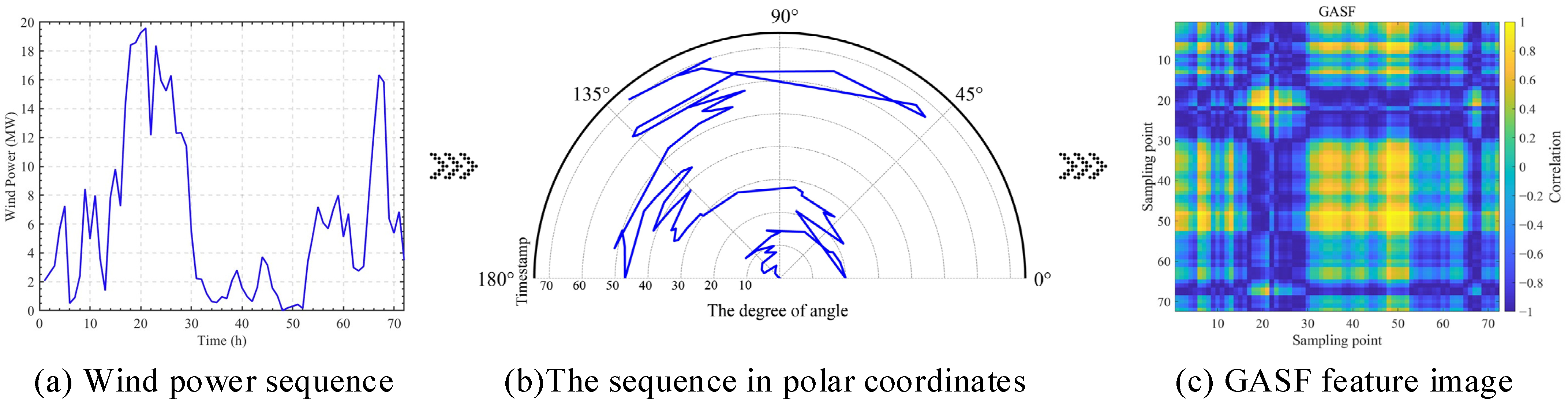
The output power of wind turbines is influenced by various meteorological factors, and utilizing meteorological data as inputs for prediction can effectively enhance the generalization and accuracy of the prediction model. However, not all weather features in the raw data necessarily exert a significant impact on wind power. Including redundant input variables not only increases the training runtime of the model but also potentially diminishes its prediction accuracy. Therefore, in this study, conducting correlation analysis between input feature quantities and reconstructed modal sequences becomes crucial for improving the accuracy of submodal prediction results.
Compared to other methods of calculating correlation, the Spearman correlation coefficient method is unaffected by the overall distributions of data and sample sizes, making it more suitable for analyzing correlations between time-series data of equal length and non-normally distributed nature [25]. Therefore, in this study, we employed the Spearman correlation coefficient to determine the relationship between modal components of wind power series and meteorological characteristic variables [26], as follows:
ρ X Y = i = 1 n ( x i x ¯ ) ( y i y ¯ ) i = 1 n x i x ¯ 2 i = 1 n y i y ¯ 2 ,
where the variable n represents the length of the sequence. In addition, x ¯ and y ¯ indicate the average values of the original sequence X and Y converted into the rank sequence x and y , respectively. The absolute value of ρ X Y can be utilized to assess the strength of correlation among these variables, with larger values indicating a stronger correlation.

2.4. GASF

Time-domain analysis provides a comprehensive representation of the signal, but the conventional approach of converting one-dimensional signals into two-dimensional images fails to fully capture their temporal correlation. In contrast, the GASF method transforms wind power signals into two-dimensional color images, enabling machine vision techniques to explore short time-series features and correlation patterns at different time points. This image-based representation effectively preserves the temporal dependence [3].
A GASF encodes one-dimensional time-series signals into two-dimensional matrices by transforming them in polar coordinates, resulting in images. For a time series X = { x 1 , x 2 , , x n } with n points, the transformation process of a GASF for sequence X is as follows [20].
(1)
Firstly, the time series X values are normalized to the interval [−1, 1] using Equation (16), as follows:
  x ~ i = [ x i m a x ( X ) ] + [ x i m i n ( X ) ] m a x ( X ) m i n ( X ) ,
where x i is the i th ( i = 1,2 , , n ) sampled signal, and x ~ i is the normalized value of x i .
(2)
The normalized time series X ~ = { x ~ 1 , x ~ 2 , , x ~ n } values are transformed in polar coordinates by Equation (17), as follows:
  θ i = a r c c o s x ~ i r i = t i / N ,
where θ i is the angular cosine of the polar coordinates; r i is the radius; t i is the timestamp; and N is a constant factor of the span of the regularized polar coordinate system.
(3)
In the polar coordinate system ϕ, the cosine and angle values are calculated for each polar coordinate, and the encoded results are input into a matrix using Equation (18), as follows:
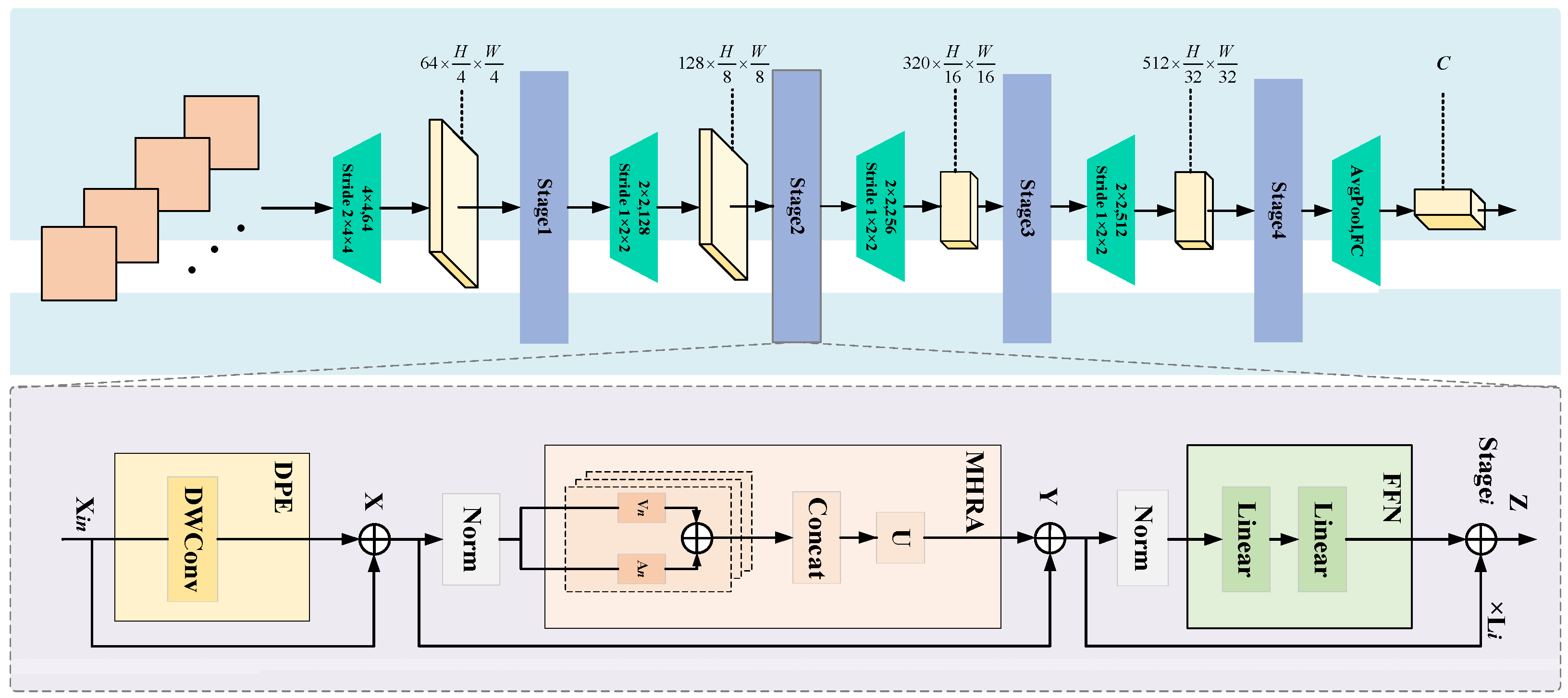
  G A S F = c o s ( ϕ 1 + ϕ 1 ) c o s ( ϕ 1 + ϕ n ) c o s ( ϕ n + ϕ 1 ) c o s ( ϕ n + ϕ n ) .
The matrix operation is performed in the form of an inner product, and the main diagonal of the matrix includes the original direction and angle information of the time-domain mapped signal. Then, transform the GASF matrix into a two-dimensional GASF image and establish its absolute temporal relationship in polar coordinates.
Figure 2 illustrates the conversion of one-dimensional signals into GASF process. Figure 2a displays the random wind power time-series signals with a sampling interval of 1 h and a total of 72 sampling points over three days; Figure 2b shows the time-series signals transformed into polar coordinates using the Equation (17); and Figure 2c presents the two-dimensional GASF image generated from the original signals through the image coding method, whereby different features, such as colors, dots, and lines, in corresponding positions can fully capture information related to the time-series signal.

2.5. UniFormer

Visual data recognition processing, such as images and videos, is plagued by inefficiencies in computation due to local redundancy and ineffective learning caused by distant global dependencies. Current mainstream visual recognition algorithms, including CNNs and Visual Transformers (ViTs), often struggle to address these challenges simultaneously. The limited acceptance field of CNNs makes it difficult for them to learn global dependencies through convolution, while the redundant attention approach of ViTs imposes an unnecessary computational burden. Building upon this foundation, the study in [27] proposed a novel UniFormer model that effectively combines convolution and self-attention in a concise transformer format. This model successfully resolves issues related to local redundancy and global dependency problems while adopting an hourglass-style design for lightweight effectiveness in visual tasks. Extensive experiments demonstrate that UniFormer exhibits robust performance on visual tasks with throughput 2–4 times higher than recent lightweight models.
Specifically, the UniFormer model comprises three essential modules: Dynamic Position Embedding (DPE), Multi-Head Relation Aggregator (MHRA), and Feed-Forward Network (FFN). The distinctive design of the relation aggregator serves as a fundamental divergence between UniFormer and conventional CNNs and ViTs. In the shallow layer, the relational aggregator captures local token affinities using a small matrix of learnable parameters, inheriting a convolutional style that effectively reduces computational redundancy through contextual aggregation of neighboring regions. At deeper levels, the relational aggregator learns global token affinities by means of token similarity comparisons, adopting self-attention mechanisms to adaptively construct long-range dependencies from distant regions or frames. Representation learning is facilitated by hierarchically overlaying local and global UniFormer blocks while flexibly integrating their collaborative capabilities. Figure 3 illustrates the schematic structure of UniFormer.
As shown in Figure 3, the UniFormer module consists of the following three key modules of DPE, MHRA and FFN, as follows:
X = D P E X i n + X i n ,  
Y = M H R A N o r m X + X ,
Z = F F N N o r m Y + Y ,
where X , Y , and Z represent the generated tensors of each layer, respectively.
Considering the input token tensor X i n R C × T × H × W (for image input T = 1), DPE is first introduced to dynamically integrate the location information into all the tokens (Equation (19)). The DPE does not require the input resolution and makes good use of the token ordering for better visual recognition. MHRA is then utilized to augment each token based on its contextual tokens through relational learning (Equation (20)). By flexibly designing token affinity at shallow and deep layers, MHRA can cleverly unify convolution and self-attention to reduce local redundancy and learn global dependencies. Finally, an FFN is added, like traditional ViTs, which consists of two linear layers and a nonlinear function GELU (Equation (21)). The number of channels is first expanded by the ratio of 4 and then recovered so that each token will be individually enhanced.
The UniFormer model integrates convolution and self-attention in a transformer architecture to address computational redundancy, capture intricate dependencies, efficiently learn local and global token relationships, and enable improved accuracy–computational trade-offs across various vision tasks spanning image to video domains.

3. Model Structure and Evaluation Metrics

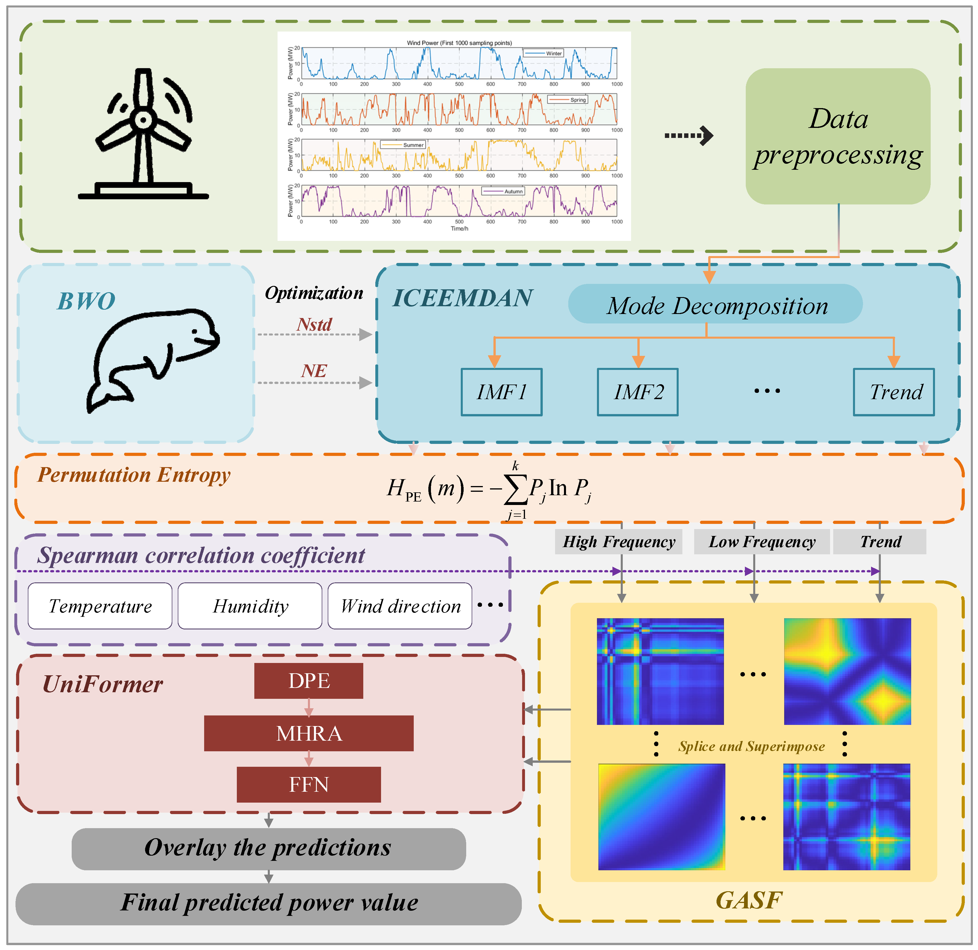
3.1. Model Structure

The BIGU prediction process is illustrated in Figure 4.
(1)
Initially, the BWO algorithm is employed to optimize the N s t d and N E parameters of the ICEEMDAN decomposition algorithm, with the minimal value of the envelope entropy of wind power sequences in different seasons serving as the fitness function. Subsequently, wind power data undergo ICEEMDAN decomposition for each season to obtain multiple submodal IMF components.
(2)
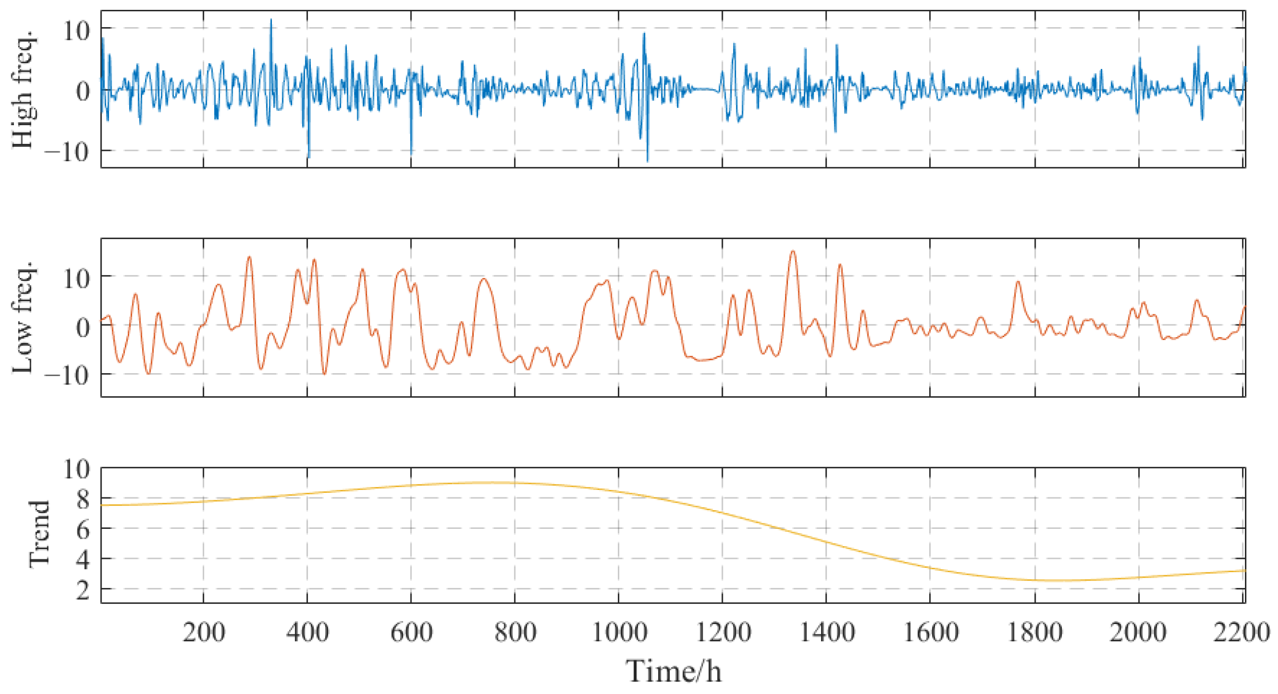
The permutation entropy value of each decomposed IMF component is calculated and used to reconstruct them into a high-frequency term, low-frequency term, and trend term (i.e., residual term).
(3)
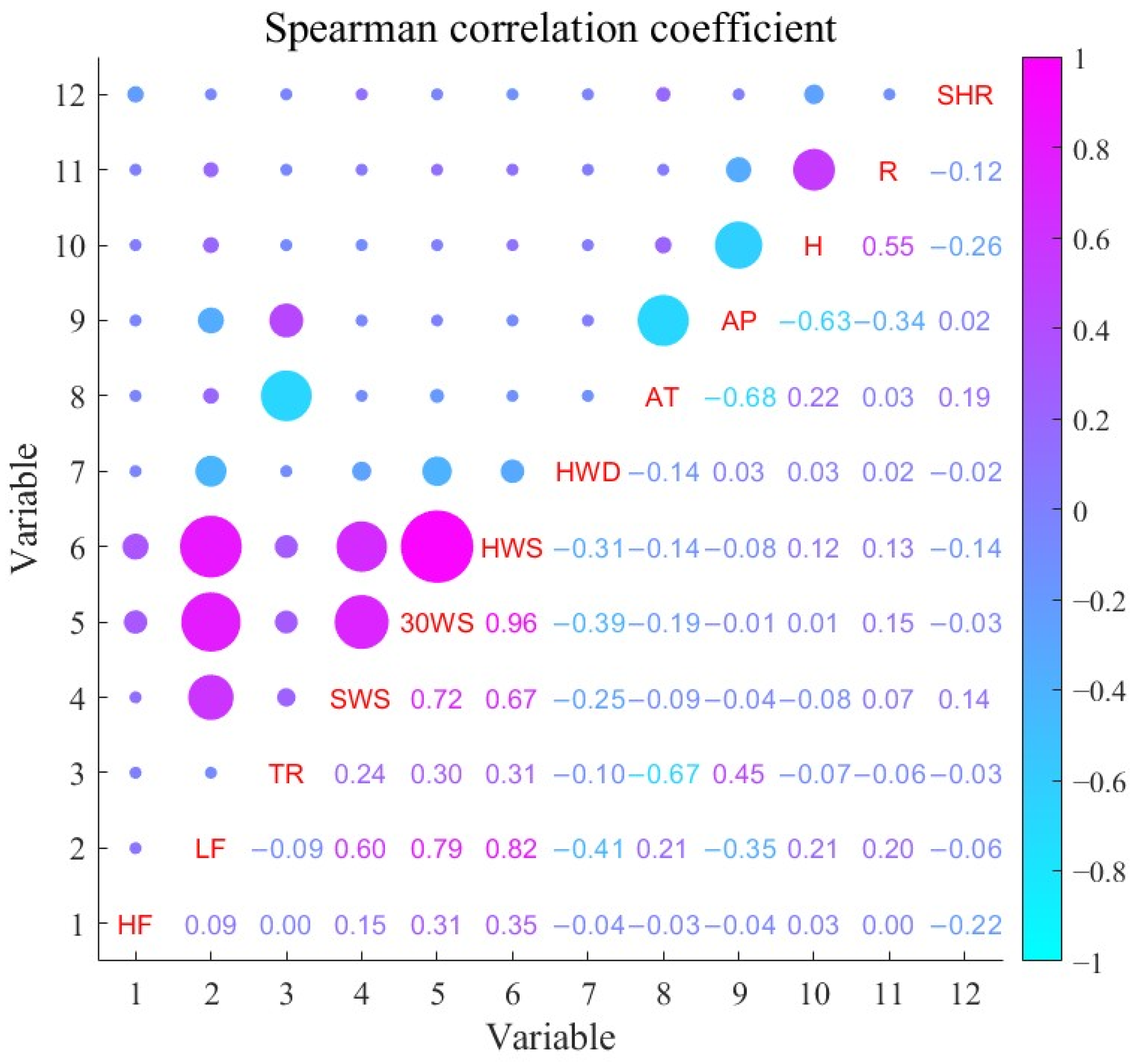
Spearman’s feature selection algorithm is utilized to correlate the reconstructed IMF components with corresponding weather features, selecting high-scoring meteorological feature vectors which are then transformed into 2D GASF images after splicing and superimposing them with their respective modal components.
(4)
The GASF feature image is inputted into the UniFormer prediction model for predicting high-frequency terms, low-frequency terms, and trend terms separately before combining all prediction results.

3.2. Evaluation Metrics

In order to provide a more comprehensive assessment of the model’s predictive accuracy, we employed the Mean Absolute Error (MAE), Root Mean Square Error (RMSE), and R (Correlation Coefficient) as evaluation metrics. The corresponding calculation formulas are presented below:
M A E = 1 n i = 1 n | y p y r | ,
R M S E = 1 n i = 1 n ( y p y r ) 2 ,
R = i = 1 n ( y p y p ¯ ) ( y r y r ¯ ) i = 1 n ( y p y p ¯ ) 2 × i = 1 n ( y r y r ¯ ) 2 ,
where n is the number of predicted samples, y p is the predicted value of the model, y r is the true value, y p ¯ is the mean value of the true data, and y r ¯ is the mean value of the predicted data. MAE and RMSE are mainly used to measure the deviation between the predicted value and the actual value, and the smaller the value, the higher the accuracy of the model’s prediction; the correlation coefficient, R, measures the linear correlation between the predicted value and true value. The closer the value of R is to 1, the better the prediction effect.

4. Case Study I

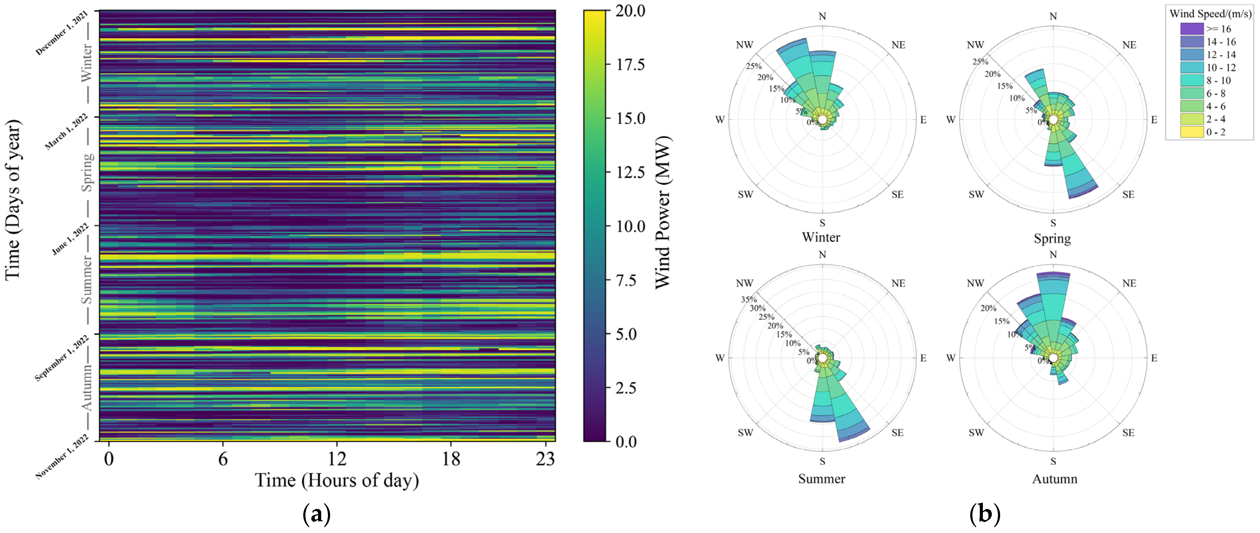
4.1. Data Description

In order to validate the proposed model in this paper, wind power data from a coastal wind farm in East China spanning from 1 December 2021 to 30 November 2022, along with measured meteorological data from local meteorological stations, were utilized as experimental samples for analysis. The wind turbine’s hub height at the wind farm was set at 110 m with a total installed capacity of 20 MW. The data sampling interval was set at every hour, resulting in a total of 8760 data points over the course of one year. Table 1 presents the units and abbreviations used for the meteorological data.
The heat map in Figure 5a illustrates the spatial distribution of the wind power throughout the year. The wind farm is situated in a region characterized by four distinct seasons, namely, spring (March–May), summer (June–August), autumn (September–November), and winter (December–February). Figure 5b presents a rose diagram showcasing the variations in wind direction across these four seasons. It is evident from Figure 5b that both the wind speed and direction exhibited diverse trends and patterns across different seasons. Considering that the correlation between the decomposed modal components of wind power and meteorological factors such as wind direction varies with each season, it becomes convenient to visually compare datasets divided into these four seasons for validating the prediction efficacy of the BIGU model and comprehensively evaluating its performance on predicting seasonal variations in wind power datasets. To achieve this, we divided our prediction dataset into a training set, validation set, and test set using an 8:1:1 ratio.
The coefficient of variation, c v , is defined to quantify the distribution pattern and relative degree of fluctuation in wind speed series across different seasons [28], as wind speed exhibits distinct seasonal variations. A larger c v indicates a greater magnitude of dataset fluctuations. The formula for calculating c v is as follows:
  c v = σ μ μ = 1 n i = 1 n x i σ = 1 n i = 1 n ( x i μ ) 2 ,
where n is the number of sequences, x i is the i th sequence value, μ is the sequence mean, and σ is the sequence standard deviation.
The wind speed characteristics of the turbine hub height in different seasons are shown in Table 2.
The dataset exhibits minimal variation in winter, summer, and autumn based on the mean value, while spring demonstrates the largest coefficient of variation with significant fluctuations in wind speed. Therefore, this study selects spring as an exemplar due to its pronounced degree of fluctuation within the series for validating the predictive efficacy of our model.

4.2. Model Parameter Settings

The optimal main structure and parameter settings for achieving the best performance of the BIGU, as determined through repeated optimization testing, are presented in Table 3.
In order to verify the effectiveness of the proposed model, two-dimensional image timing prediction models, a CNN [29] and ViT [30] (based on the same GASF training image as the proposed model), were selected. The classic machine learning model ARIMA (Autoregressive Integrated Moving Average Model) [31] and deep learning prediction models LSTM [32] and GRU [33] served as baseline prediction models. Table 4 shows descriptions of the baseline model’s principles and properties. The predicted results are the average values of ten experimental runs.
The experiments in this study were conducted on an Intel(R) Core(TM) i7-13620H (4.9 GHz) processor with 32 GB RAM (Intel, Santa Clara, CA, USA), running a 64-bit Windows operating system (Microsoft, Redmond, DC, USA). The proposed main algorithmic model was implemented using frameworks, such as Tensorflow and Keras, and coded in Python.

4.3. Prediction Process

4.3.1. Modal Decomposition

The effectiveness of the BWO algorithm in ICEEMDAN optimization was verified by comparing it with the following three classical swarm intelligence optimization algorithms: whale optimization algorithm (WOA), sparrow search algorithm (SSA), and PSO. Each algorithm had a population size and iteration times set to 8 and 10, respectively, with the minimum envelope entropy serving as the fitness function. The optimization range of N s t d was from 0.15 to 0.6, while the optimization range of N E was from 50 to 600. The optimization iteration curves for all four algorithms are presented in Figure 6.
The fitness value of BWO reached its optimum after three iterations, as shown in Figure 6. Furthermore, the optimal solution (7.1141) obtained by BWO outperformed the solutions generated by the other three algorithms, thereby demonstrating the efficiency and effectiveness of BWO in optimizing ICEEMDAN parameter selection.
After the optimization of ICEEMDAN by BWO, the values of N s t d and N E were determined as 0.15 and 158, respectively. As depicted in Figure 7, the spring wind power data were decomposed into nine IMF components and one residual component (representing the trend term) with distinct frequencies using the BWO-ICEEMDAN algorithm. These submodalities exhibited a sequential decrease in their frequencies, thereby effectively decomposing the originally volatile wind power data into submodal signals exhibiting certain regularity.

4.3.2. Modal Reconstruction

According to the ICEEMDAN decomposition results, the complexity of each modality is calculated and merged using PE theory, thereby circumventing the need for the individual prediction of each modality and mitigating the accumulation of errors in final predictions, which could potentially lead to increased error magnitudes. The PE embedding dimension m   is set at three with a delay time τ of 1 s. Table 5 presents the outcomes of the permutation entropy’s computation for each component.
According to the results of the permutation entropy analysis for each sequence, IMF1–IMF3 exhibited PE values exceeding 0.6 and were subsequently reconstructed as high-frequency (HF) terms. Conversely, IMF4–IMF9 demonstrated entropy values below 0.6 and were reconstructed as low-frequency (LF) terms. Additionally, residual represents a trend term (TR) that remained unaltered during reconstruction. The resulting reconstructed sequence is illustrated in Figure 8.

4.3.3. Feature Selection

The reconstructed IMF components underwent feature selection to enhance the model’s simplicity and prediction efficiency. The features that exhibited a relatively high Spearman correlation coefficient with the meteorological variables were chosen for inclusion. The outcomes of the feature selection process are illustrated in Figure 9.
Considering the computational speed and precision, we selected weather feature values with an absolute value of the modal correlation coefficient greater than 0.3 as inputs. The outcomes of the feature selection process are presented in Table 6.

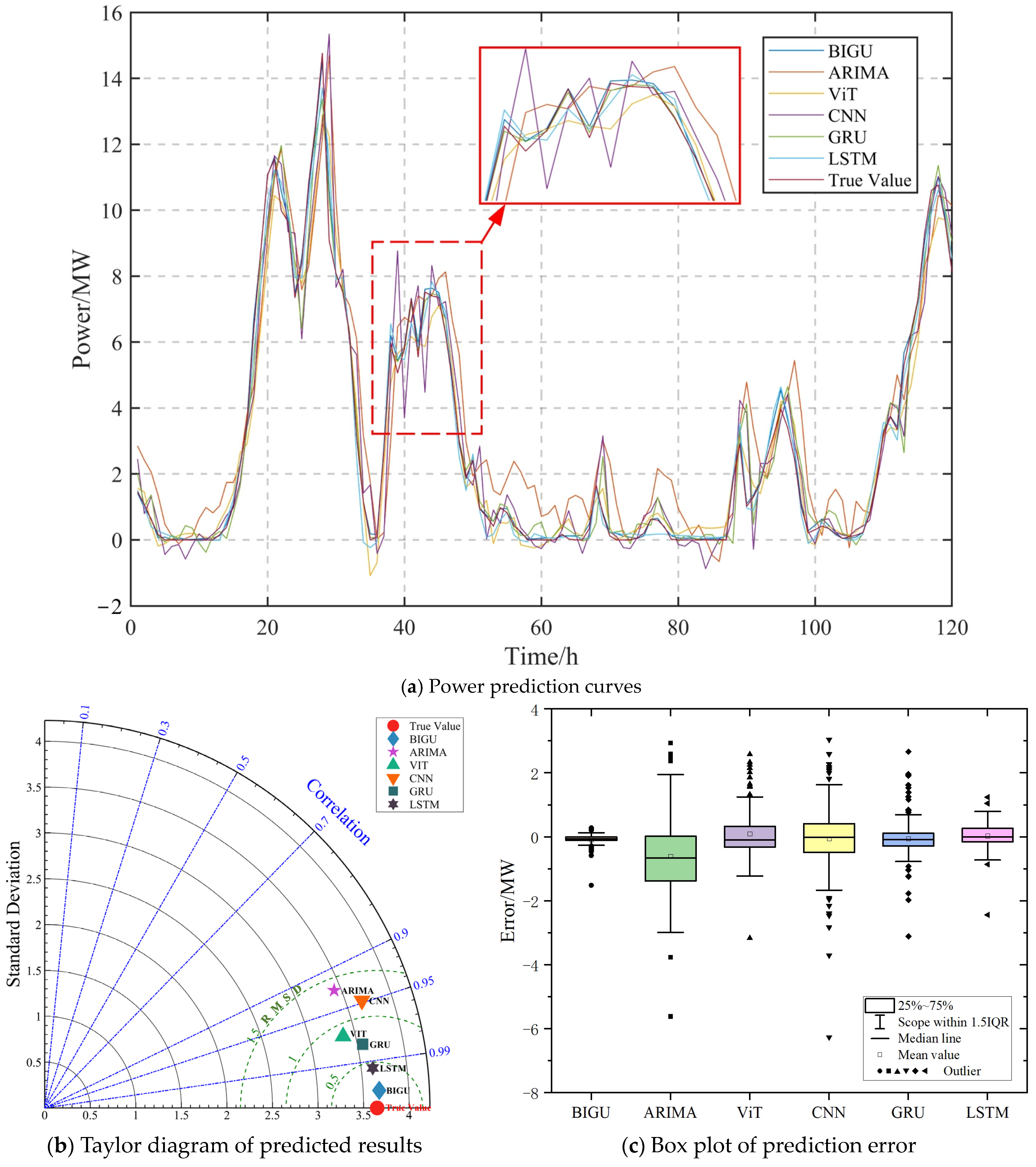
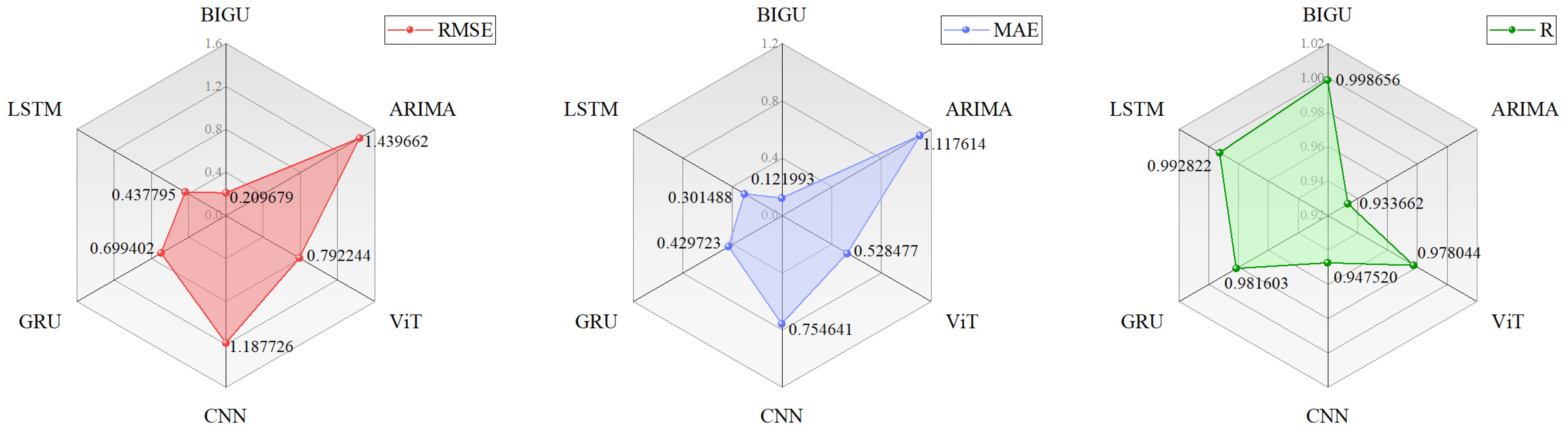
4.3.4. Predicted Results

The results of each model’s prediction for spring wind power during the last 5 days of the selected dataset are illustrated in Figure 10.
From Figure 10a, it is evident that the BIGU model proposed in this study more accurately captures the variations in peaks and troughs compared to other models, providing a better fit to the fluctuations observed in the actual wind power curve. Figure 10b presents the Taylor diagram illustrating the model prediction results, including standard deviation, correlation coefficient R, and centralized root mean squared difference (RMSD). The true value point serves as a reference for the actual wind power series. From Figure 10b, it can be observed that the BIGU model’s prediction results align closely with the radial line of R value at the reference point, indicating a high correlation between predicted values and real values. Furthermore, when considering the distance distribution of standard deviations from actual wind power data for each model, it becomes apparent that the standard deviation of the BIGU model’s predictions is closest to the reference point. This suggests that the mathematical distribution of the predicted values by our proposed model closely resembled that of the real data. The RMSD value was less influenced by outliers in the data, making it a more objective measure of the average deviation between the predicted and actual values. From the results, it is evident that BIGU exhibited lower absolute deviations and overall better prediction accuracy compared to the other models. Among these comparative models, the LSTM demonstrated superior predictive performance, highlighting its ability to effectively handle nonlinear wind power generation data across various time scales. While the GRU also achieved relatively accurate predictions compared to the LSTM, its slightly less robust architecture limits its performance. The transformer-based ViT model exceled at capturing global correlations and complex patterns but may not be as effective as an LSTM or GRU in capturing temporal correlations inherent in time-series data like wind power fluctuations. In comparison to the ViT models, the CNNs demonstrated effectiveness in identifying local patterns and short-term dependencies within the data; however, they lack inherent capability in modeling long-term dependencies in time-series data, thereby limiting their efficacy in capturing comprehensive temporal dynamics of wind power generation. Lastly, ARIMA’s reliance on linear relationships restricts its capability to model nonlinear and intricate patterns commonly observed in wind power data; thus resulting in mediocre predictive performance relative to more sophisticated neural network models. However, despite these limitations, ARIMA’s simplicity and interpretability can offer advantages under certain circumstances.
The errors between the predicted and true values of the model are depicted in Figure 10c. The boxplot reveals a consistent median BIGU prediction error of around 0, with minimal dispersion indicated by the small range between upper and lower limits. Moreover, there are fewer outliers observed in the data, indicating less deviation between the predicted and true values.
The radar chart in Figure 11 shows the evaluation metrics for wind power prediction in spring, which includes calculating the RMSE, MAE, and R values to assess the performance of different models. From the chart, it can be observed that the BIGU model provides the smallest RMSE for predicting spring wind power, with a value of 0.209679. This is 85.44% lower than the ARIMA model, 73.53% lower than the ViT model, 82.35% lower than the CNN model, 70.02% lower than the GRU model, and 52.11% lower than the LSTM model. Similarly, the BIGU model also has the lowest MAE value of 0.121993 compared to ARIMA (89.08% reduction), ViT (76.91%), CNN (83.83%), GRU (71.61%), and LSTM (59.54%) predictions. It is worth noting that BIGU also achieves a maximum R value of 0.998656 among all models evaluated for wind power prediction in spring. The overall evaluation of the predictions on this dataset indicates that BIGU demonstrated superior predictive performance.

4.4. Comprehensive Assessment

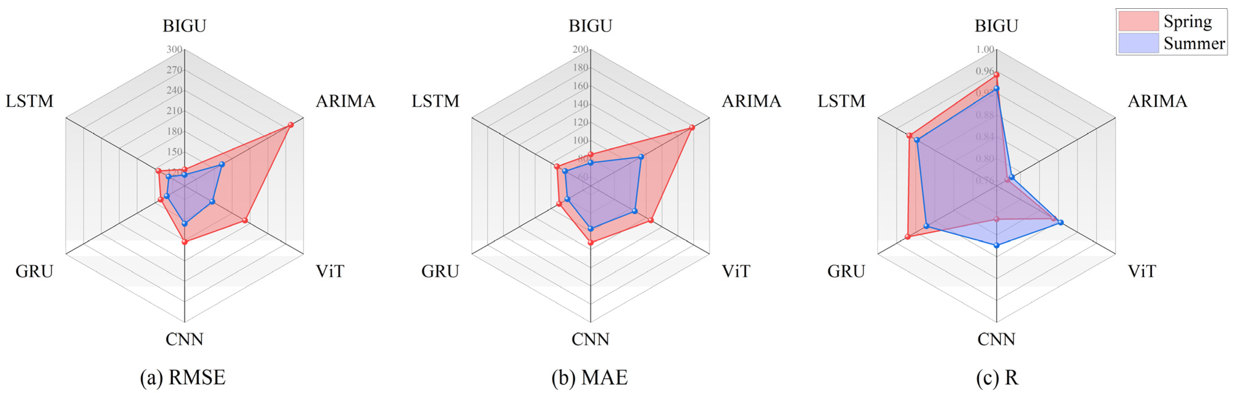
4.4.1. Summer, Autumn, and Winter Comparison

The evaluation metrics for wind power prediction in summer, autumn, and winter are presented in Table 7. From the table, it is evident that the proposed BIGU model consistently achieved optimal prediction results across all seasons. The RMSE of the BIGU prediction exhibits the smallest error among the six models, measuring 0.375476, 0.397771, and 0.336125 for summer, autumn, and winter, respectively; concurrently, the predicted MAE also demonstrates minimal values at 0.264877, 0.312885, and 0.214817, respectively. The results indicate that the BIGU model accurately captures the fluctuation characteristics of wind power, resulting in a smaller discrepancy between the predicted and original power values. The correlation coefficients (R) for summer, autumn, and winter forecasts are 0.998891, 0.998520, and 0.998922, respectively, demonstrating that compared to the comparison models, BIGU provides more precise predictions of wind power across different seasons.
The results presented above demonstrate that the BIGU model consistently outperformed other models in terms of achieving the lowest RMSE and MAE values, as well as exhibiting the highest correlation R value, for summer, autumn, and winter forecasts. This further substantiates its superiority in accurately predicting wind power and highlights its potential to effectively support applications such as power system scheduling and supply/demand balance.

4.4.2. Ablation Experiments

To validate the efficacy of ICEEMDAN decomposition and modal reconstruction in the BIGU model, ablation experiments were conducted using spring wind power as a case study, comparing the BIGU model with BIGU* (without modal reconstruction) and BIGU** (direct prediction without ICEEMDAN decomposition). This approach aims to demonstrate the significance of ICEEMDAN decomposition and subsequent modal reconstruction in enhancing wind power prediction accuracy.
In the ablation experiment, wind power prediction was conducted separately for the three models, and the corresponding prediction curves were plotted as depicted in Figure 12. From Figure 13, it is evident that the proposed BIGU model outperformed the models of BIGU* and BIGU** in terms of the evaluation metrics. BIGU achieved lower values of RMSE and MAE compared to BIGU* and BIGU**, while also demonstrating a higher correlation coefficient (R), indicating its enhanced accuracy in wind power prediction. Moreover, BIGU* clearly surpassed the model BIGU**, suggesting that although ICEEMDAN decomposition contributes to enhanced prediction accuracy, cumulative errors generated by predicting each IMF component along with model complexity still limit its effectiveness. Comparatively, the decomposed predicted model of BIGU* showed a reduction of 16.96% in RMSE, a 23.47% decrease in MAE, and an increase of 0.16% in R when compared to BIGU**. Furthermore, when compared to BIGU*, the proposed BIGU model predicted a substantial decrease of 34.70% in RMSE and 39.45% reduction in MAE alongside an increase of 0.21% in R, thus emphasizing the crucial roles played by modal decomposition and reconstruction within our proposed methodology.

5. Case Study II

5.1. Data Description

In order to further validate the effectiveness and applicability of the proposed model in wind power prediction, we selected wind power generation data from the Sotavento wind farm [34] during spring (March to May) and summer (June to August) of 2016 for analysis. The renowned Sotavento wind farm is situated in the Galicia region of northwestern Spain at the coordinates of north latitude 43.3543 and west longitude 7.8812 [14]. The original dataset comprises measurements of wind speed, wind direction, and power generation at the wheel hub of the wind farm, with a sampling interval of 10 min. The rated installed capacity during this period was 2500 kW. Missing data were corrected using an average interpolation method. Meteorological data sourced from the European Centre for Medium-Range Weather Forecasts (ECMWF), collected at hourly intervals, included various environmental variables, such as temperature, humidity, barometric pressure, and wind speed. To ensure the comparability of the experiments, the original wind power data was resampled at 1-hour intervals, and all model settings and operating environments were consistent with Case Study I. In addition, we divided the training set, validation set, and test set in an 8:1:1 ratio.

5.2. Predicted Results

Because of space constraints, the detailed forecasting process was not repeated. Table 8 presents the best BWO fitness values for the spring and summer wind power sequence decomposition, N s t d and N E values for the lowest envelope entropy, component selection during modal reconstruction, and meteorological variables for correlation selection.
It is worth mentioning that, in comparison with the other three optimization algorithms, the BWO algorithm exhibits superior convergence speed and minimal envelope entropy in both the spring and summer datasets, measuring 7.3190 and 7.2384, respectively. The N s t d and N E values for the ICEEMDAN decomposition for the spring and summer wind power sequences were 0.31 and 0.49, respectively, and 163 and 353. The PE value was used for the modal reconstruction, and meteorological variables with high correlation were selected according to the Spearman correlation coefficient method, converted into two-dimensional GASF images, and input into the BIGU model for prediction.
The evaluation indicators for the prediction results for the spring and summer datasets are presented in Figure 14. In spring, the predicted RMSE value of the BIGU model (124.150340) was 55.429892% lower than that of ARIMA with the worst performance and 11.474655% lower than that of GRU with the best performance in the comparison model. Similarly, the MAE value for the BIGU model was 84.583375, indicating minimal deviation between its predicted values and actual values. Moreover, compared to ARIMA (0.772593), ViT (0.869962), CNN (0.811128), GRU (0.936992), and LSTM (0.933531), the BIGU model achieved a higher R value (0.952931), demonstrating a superior fitting accuracy. The predicted RMSE value for the BIGU model in summer was 116.104253, which exhibits a reduction of 28.700508% compared to the ARIMA model, a decrease of 20.733483% relative to the ViT, a decline of 25.351962% when compared to the CNN, a drop of 10.679939% in comparison with the GRU, and an improvement of 8.392791% over the LSTM. Meanwhile, the MAE value (75.323717) and R value (0.928080) predicted by BIGU were both the best. Compared with other models, it is evident that BIGU still maintains the highest prediction accuracy on the spring and summer wind power dataset of Sotavento wind farm in 2016. Through meticulous experimental verification, our proposed model consistently showcased exceptional predictive accuracy on this secondary wind power dataset as well, thereby further validating its robustness and high-precision forecasting capability across diverse data environments.

6. Conclusions and Suggestions

6.1. Conclusions

The present study proposes a novel short-term wind power prediction model based on 2D pictorialization, effectively capturing the spatial pattern information of time-series data by transforming the wind power time series and its associated meteorological features into GASF images. Furthermore, feature decomposition and reconstruction were performed using the BWO-optimized ICEEMDAN algorithm. Building upon this foundation, the UniFormer model was introduced to achieve deep extraction and time-series prediction of image features. The novelty of our proposed model lies in its innovative conversion of univariate time series into images, fully leveraging the advantages of pictorial data representation.
Through experimental verification of wind power prediction using two cases, combined with comprehensive evaluation results, it is evident that the proposed BIGU prediction model exhibits significant accuracy and stability compared to traditional time-series forecasting models and classical two-dimensional image data regression models. This not only affirms the efficacy of the image-based approach in capturing and leveraging intricate patterns within time-series data but also presents novel insights and tools for future wind power forecasting.

6.2. Limitations and Future Suggestions

The method presented in this paper also exhibits certain limitations. Firstly, the introduction of GASF image transformation adds computational complexity, particularly when dealing with large-scale data. In terms of computational efficiency, computer vision prediction methods do not possess an advantage over the prediction methods for one-dimensional time-series data due to inherent model characteristics. Secondly, while the UniFormer model efficiently handles pictorial time-series data, further investigation is required to fine-tune and optimize its parameters for different prediction scenarios. Future research could explore more efficient image transformation methods, as well as more flexible model structures. Lastly, there is potential for combining the proposed method with existing models to achieve comprehensive advancements in wind power prediction.

Author Contributions

Data curation, D.Z. (Danyang Zhao); methodology, W.G.; formal analysis, W.G.; resources, D.Z. (Danyang Zhao) and L.X.; software, W.G.; validation, D.Z. (Dianqiang Zhou); writing—original draft, W.G.; writing—reviewand editing, W.G. and D.Z. (Danyang Zhao); supervision, X.T. and L.X.; visualization, W.G., T.W. and X.T. All authors have read and agreed to the published version of the manuscript.

Funding

This research study was funded by the Subproject IV of the National Key Research and Development Program of China, “Integrated Technology and Application of Multi-Energy Fusion for Water Transportation Ports and Ships (Demonstration Application)” (Project No.: SQ2021YFB2600063).

Institutional Review Board Statement

Not applicable.

Informed Consent Statement

Not applicable.

Data Availability Statement

Due to privacy requirements, the dataset from Case Study I cannot be made public. The dataset required for Case Study II can be obtained for free from https://data.mendeley.com/datasets/vtsgxnwswn/1 (accessed on 11 June 2024).

Acknowledgments

The authors would like to thank the editors and the anonymous reviewers for their insightful comments and suggestions. At the same time, the authors thank macrovector/Freepik for the design of the materials in the drawings in this article. Finally, the authors thank the Sotavento Wind Farm in Spain, Mendeley Data and ECMWF for the data support.

Conflicts of Interest

The authors declare no conflicts of interest.

References

  1. Yin, L.; Zhao, M. Inception-embedded attention memory fully-connected network for short-term wind power prediction. Appl. Soft Comput. 2023, 141, 110279. [Google Scholar] [CrossRef]
  2. Zhang, Z.; Wang, J.; Wei, D.; Luo, T.; Xia, Y. A novel ensemble system for short-term wind speed forecasting based on Two-stage Attention-Based Recurrent Neural Network. Renew. Energy 2023, 204, 11–23. [Google Scholar] [CrossRef]
  3. Wang, H.; Wang, G. The prediction model for haze pollution based on stacking framework and feature extraction of time series images. Sci. Total Environ. 2022, 839, 156003. [Google Scholar] [CrossRef] [PubMed]
  4. Niu, Y.; Wang, J.; Zhang, Z.; Yu, Y.; Liu, J. A combined interval prediction system based on fuzzy strategy and neural network for wind speed. Appl. Soft Comput. 2024, 155, 111408. [Google Scholar] [CrossRef]
  5. Zhang, Y.-M.; Wang, H. Multi-head attention-based probabilistic CNN-BiLSTM for day-ahead wind speed forecasting. Energy 2023, 278, 127865. [Google Scholar] [CrossRef]
  6. Sheng, Y.; Wang, H.; Yan, J.; Liu, Y.; Han, S. Short-term wind power prediction method based on deep clustering-improved Temporal Convolutional Network. Energy Rep. 2023, 9, 2118–2129. [Google Scholar] [CrossRef]
  7. Liu, Y.; Li, L.; Liu, J. Short-term wind power output prediction using hybrid-enhanced seagull optimization algorithm and support vector machine: A high-precision method. Int. J. Green Energy 2024, 1–14. [Google Scholar] [CrossRef]
  8. Al-qaness, M.A.A.; Ewees, A.A.; Fan, H.; Abualigah, L.; Elsheikh, A.H.; Abd Elaziz, M. Wind power prediction using random vector functional link network with capuchin search algorithm. Ain Shams Eng. J. 2023, 14, 102095. [Google Scholar] [CrossRef]
  9. Zhang, C.; Wang, Y.; Fu, Y.; Qiao, X.; Nazir, S.; Peng, T. A novel DWTimesNet-based short-term multi-step wind power forecasting model using feature selection and auto-tuning methods. Energy Convers. Manag. 2024, 301, 118045. [Google Scholar] [CrossRef]
  10. Liu, Z.; Ware, T. Capturing Spatial Influence in Wind Prediction with a Graph Convolutional Neural Network. Front. Environ. Sci. 2022, 10, 836050. [Google Scholar] [CrossRef]
  11. Wang, C.; He, Y.; Zhang, H.-L.; Ma, P. Wind power forecasting based on manifold learning and a double-layer SWLSTM model. Energy 2024, 290, 130076. [Google Scholar] [CrossRef]
  12. Wei, C.-C.; Chiang, C.-S. Assessment of Offshore Wind Power Potential and Wind Energy Prediction Using Recurrent Neural Networks. J. Mar. Sci. Eng. 2024, 12, 283. [Google Scholar] [CrossRef]
  13. Liu, X.; Zhou, J. Short-term wind power forecasting based on multivariate/multi-step LSTM with temporal feature attention mechanism. Appl. Soft Comput. 2024, 150, 111050. [Google Scholar] [CrossRef]
  14. Meng, A.; Chen, S.; Ou, Z.; Xiao, J.; Zhang, J.; Chen, S.; Zhang, Z.; Liang, R.; Zhang, Z.; Xian, Z.; et al. A novel few-shot learning approach for wind power prediction applying secondary evolutionary generative adversarial network. Energy 2022, 261, 125276. [Google Scholar] [CrossRef]
  15. Zhang, Y.; Zhao, Y.; Kong, C.; Chen, B. A new prediction method based on VMD-PRBF-ARMA-E model considering wind speed characteristic. Energy Convers. Manag. 2020, 203, 112254. [Google Scholar] [CrossRef]
  16. Lei, P.; Ma, F.; Zhu, C.; Li, T. LSTM Short-Term Wind Power Prediction Method Based on Data Preprocessing and Variational Modal Decomposition for Soft Sensors. Sensors 2024, 24, 2521. [Google Scholar] [CrossRef]
  17. Jiang, T.; Liu, Y. A short-term wind power prediction approach based on ensemble empirical mode decomposition and improved long short-term memory. Comput. Electr. Eng. 2023, 110, 108830. [Google Scholar] [CrossRef]
  18. Ai, C.; He, S.; Hu, H.; Fan, X.; Wang, W. Chaotic time series wind power interval prediction based on quadratic decomposition and intelligent optimization algorithm. Chaos Solitons Fractals 2023, 177, 114222. [Google Scholar] [CrossRef]
  19. Hu, W.; Mao, Z. Forecasting for Chaotic Time Series Based on GRP-lstm GAN Model: Application to Temperature Series of Rotary Kiln. Entropy 2022, 25, 52. [Google Scholar] [CrossRef]
  20. Tian, W.; Wu, J.; Cui, H.; Hu, T. Drought Prediction Based on Feature-Based Transfer Learning and Time Series Imaging. IEEE Access 2021, 9, 101454–101468. [Google Scholar] [CrossRef]
  21. Liu, B.; Cen, W.; Zheng, C.; Li, D.; Wang, L. A combined optimization prediction model for earth-rock dam seepage pressure using multi-machine learning fusion with decomposition data-driven. Expert Syst. Appl. 2024, 242, 122798. [Google Scholar] [CrossRef]
  22. Zhong, C.; Li, G.; Meng, Z. Beluga whale optimization: A novel nature-inspired metaheuristic algorithm. Knowl.-Based Syst. 2022, 251, 109215. [Google Scholar] [CrossRef]
  23. Bandt, C.; Pompe, B. Permutation entropy: A natural complexity measure for time series. Phys. Rev. Lett. 2002, 88, 174102. [Google Scholar] [CrossRef] [PubMed]
  24. Sun, J.; Zhao, P.; Sun, S. A new secondary decomposition-reconstruction-ensemble approach for crude oil price forecasting. Resour. Policy 2022, 77, 102762. [Google Scholar] [CrossRef]
  25. Peng, Y.; Song, D.; Qiu, L.; Wang, H.; He, X.; Liu, Q. Combined Prediction Model of Gas Concentration Based on Indicators Dynamic Optimization and Bi-LSTMs. Sensors 2023, 23, 2883. [Google Scholar] [CrossRef] [PubMed]
  26. Wang, C.; Lin, H.; Hu, H.; Yang, M.; Ma, L. A hybrid model with combined feature selection based on optimized VMD and improved multi-objective coati optimization algorithm for short-term wind power prediction. Energy 2024, 293, 30684. [Google Scholar] [CrossRef]
  27. Li, K.; Wang, Y.; Zhang, J.; Gao, P.; Song, G.; Liu, Y.; Li, H.; Qiao, Y. UniFormer: Unifying Convolution and Self-Attention for Visual Recognition. IEEE Trans. Pattern Anal. Mach. Intell. 2023, 45, 12581–12600. [Google Scholar] [CrossRef]
  28. Chaudhari, K.; Thakkar, A. Neural network systems with an integrated coefficient of variation-based feature selection for stock price and trend prediction. Expert Syst. Appl. 2023, 219, 119527. [Google Scholar] [CrossRef]
  29. Xu, M.; Mao, Y.; Yan, Z.; Zhang, M.; Xiao, D. Coal and Gangue Classification Based on Laser-Induced Breakdown Spectroscopy and Deep Learning. ACS Omega 2023, 8, 47646–47657. [Google Scholar] [CrossRef]
  30. Zhang, Z.; Li, J.; Cai, C.; Ren, J.; Xue, Y. Bearing Fault Diagnosis Based on Image Information Fusion and Vision Transformer Transfer Learning Model. Appl. Sci. 2024, 14, 2706. [Google Scholar] [CrossRef]
  31. Yu, E.; Xu, G.; Han, Y.; Li, Y. An efficient short-term wind speed prediction model based on cross-channel data integration and attention mechanisms. Energy 2022, 256, 124569. [Google Scholar] [CrossRef]
  32. Yan, Y.; Wang, X.; Ren, F.; Shao, Z.; Tian, C. Wind speed prediction using a hybrid model of EEMD and LSTM considering seasonal features. Energy Rep. 2022, 8, 8965–8980. [Google Scholar] [CrossRef]
  33. Huang, X.; Zhang, Y.; Liu, J.; Zhang, X.; Liu, S. A Short-Term Wind Power Forecasting Model Based on 3D Convolutional Neural Network–Gated Recurrent Unit. Sustainability 2023, 15, 14171. [Google Scholar] [CrossRef]
  34. Li, Y. Data for: Short-term wind power forecasting approach based on clustering algorithm and Seq2Seq model using NWP data. Mendeley Data 2021, 1. [Google Scholar] [CrossRef]
Figure 1. Behavioral stages of beluga whales.
Jmse 12 01173 g001
Figure 2. Conversion of a 1D timing signal into GASF.
Jmse 12 01173 g002
Figure 3. UniFormer’s structure.
Jmse 12 01173 g003
Figure 4. The procedure of BIGU’s wind power prediction.
Jmse 12 01173 g004
Figure 5. (a) Thermogram of wind power; (b) rose diagram of wind direction at hubs.
Jmse 12 01173 g005
Figure 6. Iterative curves of fitness for the 4 algorithms.
Jmse 12 01173 g006
Figure 7. Modal decomposition results.
Jmse 12 01173 g007
Figure 8. Modal reconstruction results.
Jmse 12 01173 g008
Figure 9. Spearman’s correlation coefficient between reconstructed modes and meteorological features.
Jmse 12 01173 g009
Figure 10. Spring wind power prediction results.
Jmse 12 01173 g010
Figure 11. Radar chart of spring wind power prediction and evaluation metrics.
Jmse 12 01173 g011
Figure 12. Prediction curves.
Jmse 12 01173 g012
Figure 13. Radar chart of ablation experimental prediction and evaluation metrics.
Jmse 12 01173 g013
Figure 14. Radar chart of spring and summer wind power prediction and evaluation metrics.
Jmse 12 01173 g014
Table 1. Meteorological variables and abbreviations for the dataset.
Meteorological VariableUnitAbbreviation
Surface horizontal wind speedm/sSWS
Horizontal wind speed at a height of 30 mm/s30 WS
Wind turbine hub wind speedm/sHWS
Wind turbine hub wind direction°HWD
Air temperature°CAT
Air pressurehPaAP
Humidity%H
Rainfallmm/hR
Surface horizontal radiationW/m2SHR
Table 2. Characteristic indicators of wind speed at hub height in different seasons.
Fluctuation IndicatorWinterSpringSummerAutumn
μ 7.0300206.5455976.9220307.416649
σ 2.9705273.1596413.2066903.388796
c v 0.4225490.4827120.4632590.456917
Table 3. Main parameter settings of BIGU.
StructureParameters
BWOPopulation size: 8
Maximum number of iterations: 10
N s t d optimization range: 0.15–0.6
N E optimization range: 50–600
GASFSampling interval: 48
UniFormerDepth = [3, 4, 8, 3]
Embedding dimension = [64, 128, 320, 512]
Head dimension = 64
Mlp ratio = 4
Loss functionMSE
OptimizerAdam
Learning rate0.0001
Time window48
Batch size32
Table 4. Baseline predictive models.
ModelDescription
CNNCNN is a deep learning model for processing grid-like topology data with powerful feature extraction capabilities, especially good at processing image data.
ViTViT splits the image into fixed-size patches and uses a self-attention mechanism to capture the relationships between the patches, which is very effective in capturing long-distance dependencies.
ARIMAARIMA is suitable for modeling and forecasting stationary time-series data through differential and autoregressive methods.
LSTMLSTM is an improved recurrent neural network (RNN), which controls information flow by introducing memory cells and gates to retain dependent information for a long time.
GRUGRU includes an update gate and reset gate, which simplifies the gating mechanism of LSTM and makes the computation more efficient.
Table 5. IMF component PE values.
ModalPE ValueModalPE Value
IMF10.9980IMF60.4369
IMF20.8440IMF70.4162
IMF30.6638IMF80.4074
IMF40.5457IMF90.3985
IMF50.4796R0.3909
Table 6. Feature selection results.
Modal ComponentSelection of Features
HF30 WS, HWS
LFSWS, 30 WS, HWS, HWD, AP
TRHWS, AT, AP
Table 7. Prediction evaluation metrics.
SeasonsModelsRMSEMAER
SummerBIGU0.3754760.2648770.998891
ARIMA1.0540930.7842700.947841
ViT0.6754430.4801760.989460
CNN0.8906680.6316270.959301
GRU0.4666590.3118910.988728
LSTM0.4451840.3096030.996183
AutumnBIGU0.3977710.3128850.998520
ARIMA1.7515701.0972570.974751
ViT1.4878741.0811970.983571
CNN1.6577941.1268660.976416
GRU1.5203181.1042900.981943
LSTM0.7276260.5006390.995559
WinterBIGU0.3361250.2148170.998922
ARIMA1.2615960.894050.980482
ViT0.9391610.6326820.988128
CNN0.9666940.6696160.98682
GRU0.5492510.3839410.996163
LSTM0.5713660.3998870.996554
Table 8. Key parameters of the modal decomposition and reconstruction.
SpringBWO Optimum Fitness Value: 7.3190
N s t d : 0.31, N E : 163
High-frequency termsReconstruction mode: IMF1–IMF3
Meteorological variables selection: HWS
Low-frequency termsReconstruction mode: IMF4–IMF9
Meteorological variables selection: HWS, SWS
Trend termMeteorological variable selection: AT
SummerBWO Optimum fitness value: 7.2384
N s t d : 0.49, N E : 353
High-frequency termsReconstruction mode: IMF1–IMF3
Meteorological variable selection: HWS
Low-frequency termsReconstruction mode: IMF4–IMF10
Meteorological variables selection: HWS, SWS
Trend termMeteorological variable selection: AT
Disclaimer/Publisher’s Note: The statements, opinions and data contained in all publications are solely those of the individual author(s) and contributor(s) and not of MDPI and/or the editor(s). MDPI and/or the editor(s) disclaim responsibility for any injury to people or property resulting from any ideas, methods, instructions or products referred to in the content.

