An Invariant Filtering Method Based on Frame Transformed for Underwater INS/DVL/PS Navigation

Abstract

Underwater vehicles heavily depend on the integration of inertial navigation with Doppler Velocity Log (DVL) for fusion-based localization. Given the constraints imposed by sensor costs, ensuring the optimization ability and robustness of fusion algorithms is of paramount importance. While filtering-based techniques such as Extended Kalman Filter (EKF) offer mature solutions to nonlinear problems, their reliance on linearization approximation may compromise final accuracy. Recently, Invariant EKF (IEKF) methods based on the concept of smooth manifolds have emerged to address this limitation. However, the optimization by matrix Lie groups must satisfy the “group affine” property to ensure state independence, which constrains the applicability of IEKF to high-precision positioning of underwater multi-sensor fusion. In this study, an alternative state-independent underwater fusion invariant filtering approach based on a two-frame group utilizing DVL, Inertial Measurement Unit (IMU), and Earth-Centered Earth-Fixed (ECEF) configuration is proposed. This methodology circumvents the necessity for group affine in the presence of biases. We account for inertial biases and DVL pole-arm effects, achieving convergence in an imperfect IEKF by either fixed observation or body observation information. Through simulations and real datasets that are time-synchronized, we demonstrate the effectiveness and robustness of the proposed algorithm.

1. Introduction

Autonomous Underwater Vehicles (AUVs) employ a diverse array of methods to determine their geographic location. This includes the use of inertial components, a Global Navigation Satellite System (GNSS) for satellite-based multipoint positioning, environmental perception through cameras and Doppler Velocity Logs (DVLs), acoustic ranging techniques for distance estimation, and pressure sensors for depth measurements. Given the limitations of electromagnetic wave propagation in the underwater environment, particularly about GNSS-based positioning and acousto-optic ranging, various fusion techniques utilizing an Inertial Navigation System (INS)/DVL have been utilized to improve the accuracy of positioning [1,2]. To overcome the nonlinear optimization challenges related to the fusion of multiple sensor sources, state estimation can be achieved using optimization methods such as the Extended Kalman Filter (EKF) or least squares techniques [3,4]. In a more complex manner, SLAM localization is achieved through data correlation and loopback detection, which can be accomplished by image sonar or underwater vision [5,6].

Nevertheless, conventional filtering techniques, which depend on the linearization of nonlinear problems, result in error accumulation, particularly noticeable in long-duration positioning tasks [7]. The property of Lie groups to maintain smooth structures on manifolds enables the effective description of robot positioning characteristics [8,9]. The Invariant Extended Kalman filter (IEKF) algorithm gives a novel solution [10,11], with applications extending to legged robots and beyond [12]. Unfortunately, for IEKF to attain trajectory-independent error with left–right invariance, the state must adhere to a group affine property. In the optimization problem of Earth frame-based navigation, researchers often introduce an auxiliary velocity vector, which leads to increased computational complexity [13,14,15,16].

Hence, drawing inspiration from [17], we propose a new method for representing observations in different coordinate systems using two frames, which enables the optimization of invariant filtering. This approach eliminates the need for auxiliary vectors and improves localization accuracy. Overall, the contributions of this paper can be delineated as follows:

• Utilizing a novel two-frame group filtering approach, along with a comprehensive formulation and validation, encompassing both fixed and body observations.
• Leveraging DVL and depth sensor data as primary observations, the methodology facilitates underwater navigation filtering, obviating the necessity for intricate transformations to satisfy group affine requirements.
• Algorithmic validation is conducted using simulated datasets and proprietary real-world underwater data, ensuring robustness and efficacy.

In the subsequent sections of this paper, we delve into specific aspects of our research. Section 2 provides an overview of recent advancements and limitations in underwater navigation optimization and the application of Lie group optimization. Section 3 presents the Lie group theory with a specific emphasis on the two-frame group theory, detailing its enhancements and application in underwater navigation. Section 4 outlines the validation process of both simulation and experimental data, followed by a comprehensive analysis and evaluation of the results in Section 5. Finally, Section 6 summarizes the whole paper and gives future research directions.

2. Related Works

2.1. Underwater Navigation Methods

With the advancement of marine science and technology, underwater navigation methods have diversified, ranging from traditional inertial navigation to acoustic localization, multi-sensor fusion navigation, and sense-calibrated navigation. For attitude estimation, Shi et al. achieved high accuracy for an INS on an underwater dynamic base using Mahalanobis distance-based outlier suppression and real-time measurement noise covariance estimation via variational Bayesian approximation [18]. Jorgensen et al. introduced a novel exogenous Kalman filter-based observer structure for attitude estimation utilizing Time Difference of Arrival (TDOA) measurements [19]. Subsequent research has focused on optimizing underwater multi-sensor fusion errors. Li et al. integrated robust navigation algorithms based on the maximum correlation entropy criterion and factor graph optimization [20]. Huang et al. used the SRAKF algorithm to compute the exact solution for the prediction error covariance matrix and measurement noise matrix, leveraging the traceless transform [21]. OuYang et al. posited an affine transformation correlation between the matched and real trajectories, estimating optimal positions using the Particle Swarm Optimization (PSO) algorithm [22]. Jin et al. formulated a mathematical model for precise alignment by utilizing the SQP algorithm to determine direction vectors and leading to rapid convergence to high-precision attitude estimation [23]. Russo et al. employed an expanded 1D convolutional layer to compress the input signal into a set of high-level features and utilized jump joins to enhance model capture [24]. This methodology facilitated attitude denoising that supports diverse filters and notably diminishes the Root Mean Square Error (RMSE).

Recently, underwater navigation has advanced to calibrate positioning errors using sensory information. Zhang et al. proposed an MBES subgraph construction method, solving error loopback issues with Frechet distance for effective SLAM data correlation [25]. Rahman et al. used a bag-of-words location recognition module for global relocation via geometric validation with PnP RANSAC [26]. Advanced deep learning methods have also been employed to adaptively learn time-varying parameters in underwater navigation. Ma et al. used deep learning to generate low-frequency position data and employed VB-based adaptive filters for navigation estimation [27]. He et al. designed a purely inertial deep learning navigation system using Convolutional Neural Network (CNN) and transformer networks for AUV motion states [28]. Li et al. achieved robust navigation during DVL failures using a NARX model [29]. Zhao et al. used a Long Short-Term Memory Network (LSTM) to process time series data, combining the accuracy of EKF with the real-time performance of federated learning (FL) to optimize underwater localization [30]. Qin et al. found that geometry-based methods typically outperform deep learning-based methods in positioning accuracy through experiments on the public underwater dataset AQUALOC [31]. Kim et al. improved INS fault diagnosis using the Nomoto model with enhanced preprocessing and input features [32].

In underwater navigation, filtering or optimization methods are employed for achieving optimal state estimation based on sensor measurements and a kinematics model. The current challenge in achieving high-precision underwater navigation is not merely selecting an optimization method and enhancing the filter’s performance sensor characteristics. Costanzi et al. proposed a method for detecting and rejecting affected measurements based on single-axis fiber optic gyro (FOG) signals, utilizing complementary filters to address magnetic perturbations from locally indistinguishable sources [33]. Ngatini et al. developed an AUV position estimation approach employing an integrated Kalman filter and a fuzzy Kalman filter (FKF) [34]. Shariati et al. tackled nonlinear state and parameter estimation by proposing a method to identify the nonlinear dynamic model of an AUV, particularly in the presence of unmeasured states [35]. Pei et al. redefined the process model using the Lie group of the constant attitude matrix between two inertial systems as states and designed a state-dependent Lie group filter [36]. Xu et al. applied the conditional adaptive gain expansion Kalman filter (CAEKF) to various sensor noise models and introduced a confidence assessment method to smooth the positioning trajectory of the AUV [37]. Fossen employed a discrete-time, unit-quaternion error-state Kalman filter to determine the position of an AUV using range measurements from a hydroacoustic network, along with improved time-delay estimation and compensation methods [38]. Comparison and conclusion of different algorithms are shown in

Table 1. Comparison of related filtering/optimization algorithms.

Author	Methodology	Conclusion
Shi et al. [18]	Variational Bayesian Robust Adaptive Kalman Filter (VBRAKF)	Error of 95.61% of KF
Huang et al. [21]	Statistical Regression Adaptive Kalman Filter (SRAKF)	93.83% improvement over UKF
Ngatini et al. [34]	Integrated Kalman Filter and Fuzzy Kalman Filter	Position error is 92% of FKF; angle error is 93% of FKF
Pei et al. [36]	State-Dependent Lie Group-based Filter	Accuracy is 70% improved over Quaternion KF
Xu et al. [37]	Conditional Adaptive gain Expansion Kalman Filter (CAEKF)	83% improvement over EKF
Proposed	Underwater Two-Frame Group IEKF	77% improvement over IEKF

.

2.2. Li Group Optimization and Application to Underwater Navigation

Utilizing non-Euclidean geometric structures to model rotation and attitude spaces, Lie groups offer a more precise characterization of kinematic constraints and attitude changes. The logarithmic mapping of Lie groups transforms elements into vectors within their tangent spaces. This mapping facilitates the conversion of group multiplication operations into vector addition operations, thereby simplifying the derivation process. Barrau, in his Ph.D. thesis, introduced the theory of detached invariant observers on Lie groups and proposed a framework that enables the optimization of nonlinear error variables controlled by linear differential equations. He further implemented local stability verification [10]. Subsequently, he proposed the invariant Kalman filtering framework [39] and demonstrated the log-linear characterization of the Inertial Measurement Unit (IMU) equation in discrete time. Additionally, he proposed a pre-integration formula based on the Lie exponential coordinates concerning noise and bias [14]. Chang et al. utilized the analytical and concrete form of manifold to derive log-linear differential equations in continuous time without any approximation and provide left-invariant and right-invariant errors within the matrix Lie group [40]. Li et al. used exponential formulas to correct the base and fuselage attitudes and linear formulas to correct the inertial navigation coefficient errors [41].

With advancements in Lie group theory in machine learning and optimization, it has become a powerful tool for optimizing inertial and fusion navigation systems. Barfoot applied Special Euclidean (SE) groups and Baker–Campbell–Hausdorff (BCH) formulations to link uncertainty with the transformation matrix, improving the description of noise-variable perturbations [42]. Brossard et al. related uncertainty to a matrix of five extended poses, providing detailed uncertainty propagation for IMU states and deriving accurate pre-integration formulas considering Earth’s rotation [15]. Pardos used Sagittal Kinematics Dividing (SKD) analysis to model humanoid robots and employed Lie groups to solve the inverse kinematic problem [8]. Roux combined an incomplete RIEKF with a CNN to dynamically optimize the measurement noise covariance matrix, enhancing the estimation of the position, velocity, and direction of a projectile [43]. Hartley derived a continuous-time right-invariant EKF (RIEKF) for the IMU/contact process model, successfully applying it to the Cassie bipedal robots [12]. Chang developed right-vector and left-vector error state models that account for Earth’s rotation and Coriolis effect, suited for arbitrarily unaligned attitude initialization, and applied them for pre-integration on the manifold [44].

Li group optimization theory has been widely applied to the initial error alignment and multi-sensor fusion problems of underwater sensor systems. Xu et al. introduced the $SO\left(3\right)$ group state-space model, utilizing the degree of variation of auxiliary parameters to detect outliers and proposed a DVL calibration method based on the $SO\left(3\right)$ [45]. Luo et al. devised a closed-loop scheme based on a linear state-space model to mitigate the effects of IMU bias, DVL lever arm, and mounting misalignment angle between the IMU and the DVL [46]. This scheme concurrently estimates and compensates for parameter errors and a body attitude matrix using Davenport’s q method, thereby enhancing vector observation accuracy. Qian et al. developed an integrated navigation Lie group error model based on Euler angles utilizing the Proper Weighting and Conditioning Strategy (PWCS) matrix of the Lie group model [47]. Additionally, Potokar et al. extended the conventional invariant measurement model to accommodate measurements that capture only a subset of the 3D state. They incorporated additional information, such as underwater depth measurements, into the IEKF framework [48].

In this work, pre-integration-based synchronization is conducted on INS, DVL, and PS data, followed by the application of the TFG method for invariant filtering. We address the limitations associated with group affine in underwater navigation filtering by employing a novel approach that preserves positioning accuracy.

3. Methodology

3.1. Lie Group Theory

The concept of Lie group encompasses the notions of both group and smooth manifold and unifies them within a mathematical framework. In the process of robot state estimation, Lie groups, mainly the special orthogonal group $SO\left(3\right)$ and the special Euclidean group $SE\left(3\right)$, are employed to represent rotational and attitude transformations, respectively.

The orientation R of a rigid body in space is typically modeled as

$$\mathrm{SO}\left(3\right)\{\mathbf{R}\in {\mathbb{R}}^{3\times 3}\mid {\mathbf{R}}^{\mathrm{T}}\mathbf{R}={\mathbf{I}}_3,det\left(\mathbf{R}\right)=1\}$$

(1)

where ${\mathbb{R}}^{3\times 3}$ denotes the set of $3\times 3$ vectors.

For the transformation matrix, which contains the rotation matrix R and the translation vector t, it is denoted by [49]

$$SE\left(3\right)=\left\{\mathit{T}=\left[\begin{array}{cc}\mathit{R}& t\\ 0& 1\end{array}\right]\in {\mathbb{R}}^{4\times 4}|\mathit{R}\in SO\left(3\right),t\in {\mathbb{R}}^3\right\}$$

(2)

For the extended pose containing position P, velocity V, and direction R, it is expressed by

$$S{E}_2\left(3\right)\left\{\left.\mathit{T}=\left(\begin{array}{ccc}\mathit{R}& \mathit{V}& \mathit{P}\\ 0_{1,3}& 1& 0\\ 0_{1,3}& 0& 1\end{array}\right)\right|(\mathit{R},\mathit{V},\mathit{P})\in SO\left(3\right)\times {\mathbb{R}}^3\right\}$$

(3)

where $S{E}_2\left(3\right)$ is called the “double direct isometric group” [50]. Matrix multiplication provides the group composition of two elements of $S{E}_2\left(3\right)$.

A Lie algebra resides within a vector space and corresponds to a Lie group structure. The Lie algebras $so\left(3\right)$ and $se\left(3\right)$ corresponding to $SO\left(3\right)$ and $SE\left(3\right)$ are, respectively,

$$so\left(3\right)=\{\varphi \in {\mathbb{R}}^3,\left({\varphi }_{\times }\right)\in {\mathbb{R}}^{3\times 3}\}$$

(4)

$$\left.se\left(3\right)=\left\{\xi =\left[\begin{array}{c}\varphi \\ \rho \end{array}\right]\right.\in {\mathbb{R}}^6,\varphi \in so\left(3\right),\rho \in {\mathbb{R}}^3,{\xi }^{\wedge }=\left[\begin{array}{cc}\left({\varphi }_{\times }\right)& \rho \\ 0^T& 0\end{array}\right]\in {\mathbb{R}}^{4\times 4}\right\}$$

(5)

where $\varphi$ represents a three-dimensional rotation vector, × denotes the antisymmetric matrix operation applied to a three-dimensional rotation vector, and $\rho$ is a three-dimensional translation vector. It is noteworthy that, in $se\left(3\right)$, the symbol ∧ is extended to convert a six-dimensional vector to a four-dimensional matrix. Conversely, in $so\left(3\right)$, the antisymmetric matrix is commonly denoted by either ∧ or ×.

As in classical Lie group theory, small perturbations of extended posets can be described in terms of elements of the Lie algebra $S{E}_2\left(3\right)$. The operator ∧ similarly represents a linear mapping operation that transforms the elements $\xi {({\varphi }^T,{\mathbf{v}}^T,{\rho }^T)}^T\in {\mathbb{R}}^9$ into elements of the Lie algebra, as follows:

$${\xi }^{\wedge }{\left(\begin{array}{c}\varphi \\ v\\ \rho \end{array}\right)}^{\wedge }=\left(\begin{array}{ccc}\left({\varphi }_{\times }\right)& v& \rho \\ {\mathbf{0}}_{1\times 3}& 0& 0\\ {\mathbf{0}}_{1\times 3}& 0& 0\end{array}\right)$$

(6)

The exponential mapping conveniently maps small perturbations encoded in $R^9$ to $S{E}_2\left(3\right)$. For the matrix Lie group, it is defined as $exp\left(\xi \right):=ex{p}_m\left({\xi }^{\wedge }\right)$, where $ex{p}_m(·)$ denotes the classical matrix exponential mapping.

The Lie algebra space of $S{E}_2\left(3\right)$ is equivalent to the nine-dimensional Euclidean space represented as an operation. Its Lie algebra and Lie group can be expressed by the exponential map $exp(·)$ and the logarithmic map $log(·)$ as follows:

$$\chi =ex{p}_m\left({\xi }^{\wedge }\right)=\left[\begin{array}{ccc}{exp}_m\left({\varphi }_{\times }\right)& J_{l}v& J_l\rho \\ 0_{1\times 3}& 1& 0\\ 0_{1\times 3}& 0& 1\end{array}\right]$$

(7)

$$\xi =log\left(\chi \right)=\left[\begin{array}{c}\theta a\\ J_l^{-1}v\\ J_l^{-1}\rho \end{array}\right]$$

(8)

When $\theta$ is a small angle, ${exp}_m\left({\varphi }_{\times }\right)\approx {\mathrm{I}}_3+\left({\varphi }_{\times }\right)$. $j_l$ and $j_l^{-1}$ are given by the following equation:

$$J_l=\frac{sin\theta }{\theta }{I}_3+\left(1-\frac{sin\theta }{\theta }\right)a{a}^T+\left(\frac{1-cos\theta }{\theta }\right)\left(a_{\times }\right)$$

(9)

$$J_l^{-1}=\frac{\theta }{2}\frac{cot\theta }{2}{I}_3+\left(1-\frac{\theta }{2}\frac{cot\theta }{2}\right)a{a}^T-\frac{\theta }{2\left(a_{\times }\right)}$$

(10)

The BCH formula shows that, for ${\xi }_1,{\xi }_2\in {\mathbb{R}}^9$, there is $exp\left({\xi }_1\right)exp\left({\xi }_2\right)\approx exp({\xi }_1+{\xi }_2)$. The so-called concomitant operator is defined by analogy with SE (3) as

$$A{d}_T=\left(\begin{array}{ccc}R& 0_{3,3}& 0_{3,3}\\ {\left(V\right)}_{\times }R& R& 0_{3,3}\\ {\left(P\right)}_{\times }R& 0_{3,3}& R\end{array}\right)\in {\mathbb{R}}^{9\times 9}$$

(11)

The system demonstrates a property known as group affine, as the deterministic dynamical model adheres to the following criterion:

$$f_u\left(\chi \tilde{\chi }\right)=f_u\left(\chi \right)\chi +\chi f_u\left(\tilde{\chi }\right)-\chi \widetilde{f_u\left(I\right)\chi }$$

(12)

Dynamic systems that adhere to the aforementioned relations are classified as exhibiting group affine dynamics. A notable characteristic of group affine dynamics is the independence of its error state model from the global state estimate. Specifically, both the left-invariant error and the right-invariant error remain unaffected by the trajectory.

3.2. Two Frame Groups

In addressing the multi-source data fusion navigation problem, particularly in fusion with other observation sensors, the formulation often encompasses various coordinate systems. These include the inertial coordinate system (i system), the navigation coordinate system (n system), and the Earth coordinate system (e system), among others [51]. For the characterization of underwater vehicle motion, a fixed navigation frame and a time-varying self-frame are typically defined [17]. Here, the state space is designated by

$$\chi ={(R,x,X)}^T$$

(13)

where the rotation matrix $R_n$ signifies the transformation mapping vectors represented in the body frame to the world frame at time step n. Notably, x denotes variables within the fixed frame, while X represents variables within the body frame. In a product space $G\times V\times B$, where $R\in G$, $x\in V$, and $X\in B$,

Define the ∗ operator as of G on W, where the vector space $W={\mathbb{R}}^{Nd}$; i.e., W is an N-vector tuple of ${\mathbb{R}}^d$, as follows:

$$R\ast (x^1,\dots ,x^N):=(R{x}^1,\dots ,R{x}^N)$$

(14)

Define the natural output in the fixed frame and body frame as follows:

$$\left\{\begin{array}{ccc}\mathrm{Fixed}-\mathrm{frame}:\hfill & \hfill & h(R,x,X)=H_x^x+R\ast [H_X^X+B]\hfill \\ \mathrm{Body}-\mathrm{frame}:\hfill & \hfill & H(R,x,X)=R^{-1}\ast [b-H^{x}x]-H_X^X\hfill \end{array}\right.$$

(15)

Define discrete-time natural vector dynamics as ${\chi }_n=f_n({\chi }_n-1)$, where

$$f_n\left(\begin{array}{c}R\\ x\\ X\end{array}\right)=\left(\begin{array}{c}R\\ [F_{n}x+d_n]+R\ast [C_{n}X+U_n]\\ [{\Phi }_{n}X+{\mathcal{D}}_n]+R^{-1}\ast [{\Gamma }_{n}x+u_n]\end{array}\right)$$

(16)

where the matrices $F_n:V\mapsto V$, ${\varphi }_n:B\mapsto B$, $C_n:B\mapsto V$, and ${\Gamma }_n:V\mapsto B$ are all exchanged under the action of G.

Define the natural frame dynamics as ${\chi }_n=s_n({\chi }_n-1)$, where

$$s_n\left(\begin{array}{c}R\\ x\\ X\end{array}\right)=\left(\begin{array}{c}{s}_n^R\left(\chi \right)\\ x\\ X\end{array}\right)=\left(\begin{array}{c}{O}_{n}R{\Omega }_n\\ x\\ X\end{array}\right)$$

(17)

where ${\Omega }_n\in G$ has known elements.

Define a natural two-frame observed system as follows:

$$\begin{array}{c}{\chi }_n=s_n\circ f_n\left({\chi }_{n-1}\right)\hfill \\ y_n=h_n\left({\chi }_n\right)\mathrm{or}{\mathrm{Y}}_n={\mathrm{H}}_n\left({\chi }_n\right)\hfill \end{array}$$

(18)

Define the group structure on the two-frame state space $G\times V\times B$ as follows:

$$\left(\begin{array}{c}{R}_1\\ x_1\\ X_1\end{array}\right)•\left(\begin{array}{c}{R}_2\\ x_2\\ X_2\end{array}\right)=\left(\begin{array}{c}{R}_1{R}_2\\ x_1+R_1\ast x_2\\ X_2+R_2^{-1}\ast X_1\end{array}\right)$$

(19)

where those having the structure $G\times V\times B$ are denoted by $G_{V,B}^{+}$.

Define the group action on the output space in terms of the operator ⋆ as follows:

$$\begin{array}{cc}\hfill G_{V,B}^{+}\times {\rm Y}& \mapsto {\rm Y}\hfill \\ \hfill (R,x,\mathbf{x})\star \beta & =H^{x}x+R\ast \left[H^x\mathrm{X}+\beta \right]\hfill \end{array}$$

(20)

For ${\chi }_n={\varphi }_n({\chi }_{(}n-1))$ and ${\chi }_1,{\chi }_2\in G_{V,B}^{+}$, if ${\phi }_n:G_{V,B}^{+}\to G_{V,B}^{+}$:

$${\varphi }_n({\chi }_1•{\chi }_2)={\varphi }_n\left({\chi }_1\right)•{\varphi }_n{\left(Id\right)}^{-1}•{\varphi }_n\left({\chi }_2\right)$$

(21)

Then the dynamics are considered to satisfy the “group affine property”.

3.3. Two Frame Groups IEKF

A linear observational system on a group is a dynamical system observed by measuring $y_n$ or $Y_n$, denoted as follows:

$$\left\{\begin{array}{ccc}\mathrm{Left}\mathrm{action}\mathrm{case}:& {\chi }_n={\varphi }_n\left({\chi }_{n-1}\right)& y_n={\chi }_n\star b\\ \mathrm{Right}\mathrm{action}\mathrm{case}:& {\chi }_n={\varphi }_n\left({\chi }_{n-1}\right)& Y_n={\chi }_n^{-1}\star b\end{array}\right.$$

(22)

where ${\varphi }_n$ satisfies the group affine property.

Building alternative innovation terms,

$$Z_n={\widehat{\chi }}_{n|n-1}^{-1}\star y_n-b\mathrm{or}{z}_n={\widehat{\chi }}_{n|n-1}\star {\mathrm{Y}}_n-b$$

(23)

The propagation and update steps of a linear observer are defined as follows:

$$\left\{\begin{array}{cc}\mathrm{Propagation}\mathrm{step}:& {\widehat{\chi }}_{n|n-1}={\varphi }_n\left({\widehat{\chi }}_{n-1|n-1}\right)\\ \mathrm{Update}\mathrm{step}:& \left\{\begin{array}{c}{\widehat{\chi }}_{n|n}={\widehat{\chi }}_{n|n-1}·L_n\left(Z_n\right)\\ {\widehat{\chi }}_{n|n}=L_n\left(z_n\right)·{\widehat{\chi }}_{n|n-1}\end{array}\right.\end{array}\right.$$

(24)

The left-invariant error variable and the right-invariant error variable are denoted as follows:

$$\left\{\begin{array}{c}{E}_{n|n}={\widehat{\chi }}_{n|n}^{-1}·{\chi }_n\\ e_{n|n}={\chi }_n·{\widehat{\chi }}_{n|n}^{-1}\end{array}\right.$$

(25)

The updated terms for IEKF are as follows:

$$\left\{\begin{array}{c}{L}_n\left(Z_n\right)={exp}_{G_{V,B}^{+}}\left(K_n{Z}_n\right)\\ L_n\left(z_n\right)={exp}_{G_{V,B}^{+}}\left(K_n{z}_n\right)\end{array}\right.$$

(26)

where $ex{p}_{G_{V,B}^{+}}$ is the exponential mapping of TFG and $K_n$ represents Kalman gain.

The linearization error is defined as follows:

$$\left\{\begin{array}{c}{\xi }_{n|n-1}=A_n^s{A}_n^v{\xi }_{n-1|n-1}\\ {\xi }_{n|n}=(I-K_n{H}_n){\xi }_{n|n-1}\end{array}\right.$$

(27)

where the Jacobi matrices as $A_n^s$, $A_n^v$, and $H_n$ correspond to the frame dynamics, vector dynamics, and output mapping, respectively, tuned by the following Riccati equations.

The gain of TFG-IEKF is tuned using the following equation, and the final solution is shown in Figure 1.

$$\left\{\begin{array}{c}\begin{array}{cc}\hfill P_{n|n-1}=& A_n^s{A}_n^v{P}_{n-1|n-1}{\left(A_n^s{A}_n^v\right)}^T+{\widehat{\mathit{Q}}}_n\hfill \\ \hfill {\mathbf{s}}_n=& H_n{P}_{n|n-1}{H}_n^T+{\widehat{N}}_n\hfill \\ \hfill K_n=& P_{n|n-1}{H}_n^T{S}_n^{-1}\hfill \\ \hfill P_{n|n}=& (I-K_n{H}_n)P_{n|n-1}\hfill \end{array}\hfill \end{array}\right.$$

(28)

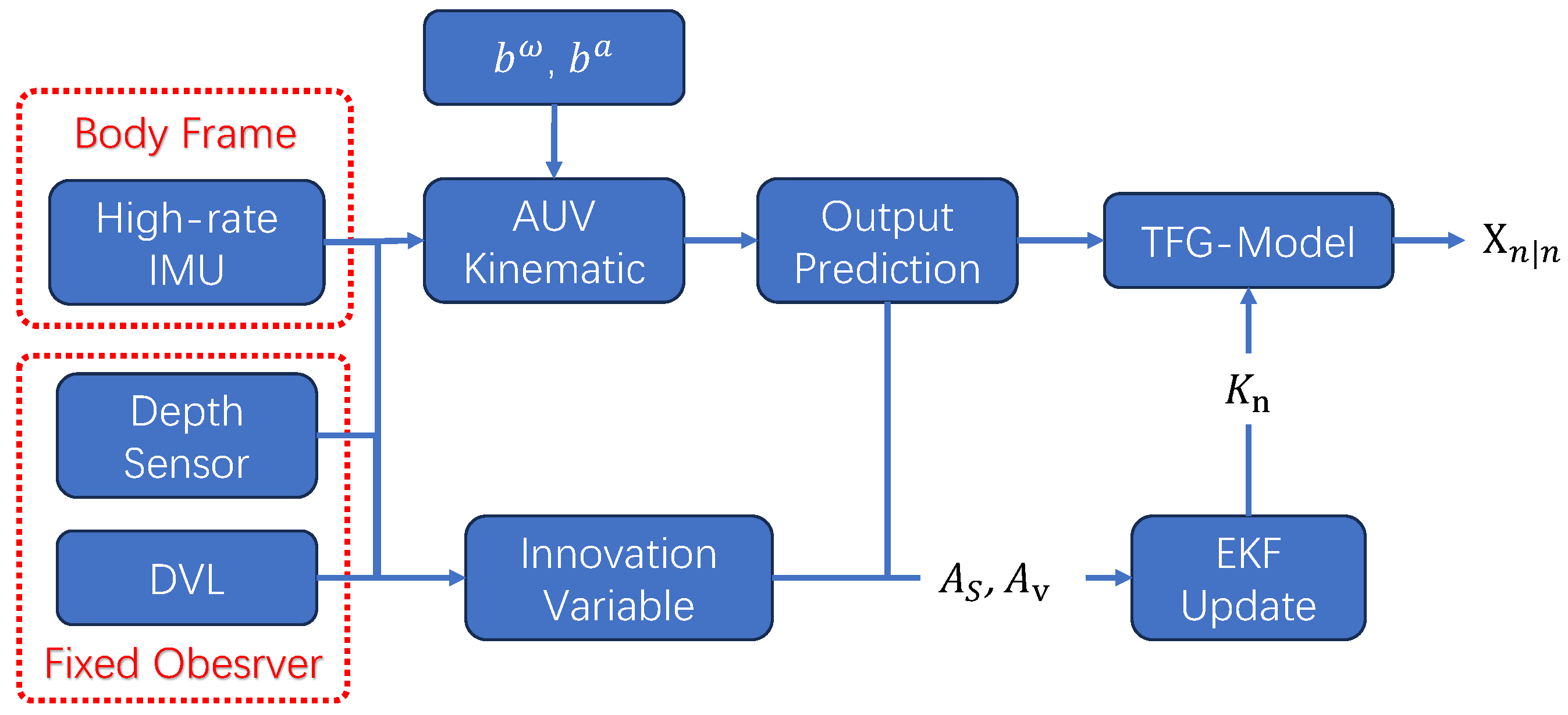
3.4. Algorithmic Implementation

The innovation variable is associated with the fixed frame output as follows:

$$\left\{\begin{array}{c}\begin{array}{cc}\hfill Z_n& ={\widehat{R}}_{n|n-1}^{-1}\ast (y_n-H^x{\widehat{x}}_{n|n-1})-H^{\mathrm{X}}{\widehat{\mathrm{X}}}_{n|n-1}-{\mathrm{B}}_n\hfill \\ \hfill z_n& ={\widehat{R}}_{n|n-1}\ast \left({\mathrm{Y}}_n+H^{\mathrm{X}}{\widehat{\mathrm{X}}}_{n|n-1}\right)+H^x{\widehat{x}}_{n|n-1}-b_n\hfill \end{array}\hfill \end{array}\right.$$

(29)

After applying vector dynamics and frame dynamics and considering observations, respectively, the estimate of moment n is expressed as ${\widehat{\chi }}_{n^{-}|n-1}$, ${\widehat{\chi }}_{n|n-1}$ and ${\widehat{\chi }}_{n|n}$. Then, the fixed frame observer of the left-invariant observer is implemented as follows:

$$\left\{\begin{array}{c}{\widehat{\chi }}_{n-|n-1}=f_n\left({\widehat{\chi }}_{n-1|n-1}\right)\hfill \\ {\widehat{\chi }}_{n|n-1}=s_n\left({\widehat{\chi }}_{n-|n-1}\right)\hfill \\ {\widehat{\chi }}_{n|n}=\left(\begin{array}{c}{\widehat{R}}_{n|n-1}{L}_n^R\left({\mathrm{Z}}_n\right)\\ {\widehat{x}}_{n|n-1}+{\widehat{R}}_{n|n-1}\ast L_n^x\left({\mathrm{Z}}_n\right)\\ L_n^X\left({\mathrm{Z}}_n\right)+L_n^R{\left({\mathrm{Z}}_n\right)}^{-1}\ast {\widehat{\mathrm{X}}}_{n|n-1}\end{array}\right)\hfill \end{array}\right.$$

(30)

Similarly, under the observation of the body frame, the constant observation value is written as follows:

$$\left\{\begin{array}{c}{\widehat{\chi }}_{n-|n-1}=f_n\left({\widehat{\chi }}_{n-1|n-1}\right)\hfill \\ {\widehat{\chi }}_{n|n-1}=s_n\left({\widehat{\chi }}_{n-|n-1}\right)\hfill \\ {\widehat{\chi }}_{n|n}=\left(\begin{array}{c}{L}_n^R\left(z_n\right){\widehat{R}}_{n|n-1}\\ L_n^x\left(z_n\right)+L_n^R\left(z_n\right)\ast {\widehat{x}}_{n|n-1}\\ {\widehat{X}}_{n|n-1}+{\widehat{R}}_{n|n-1}^{-1}\ast L_n^X\left(z_n\right)\end{array}\right)\hfill \end{array}\right.$$

(31)

Rewrite the left invariant error $E_{n|n}$ using the TFG method as follows:

$$E_{n|n}=\left(\begin{array}{c}{\widehat{R}}_{n|n}^{-1}{R}_n\\ {\widehat{R}}_{n|n}^{-1}\ast (x_n-{\widehat{x}}_{n|n})\\ {\mathrm{X}}_n-\left(R_n^{-1}{\widehat{R}}_{n|n}\right)\ast {\widehat{\mathrm{X}}}_{n|n}\end{array}\right)$$

(32)

Similarly, the right invariant error is represented in the body frame as follows:

$$e_{n|n}=\left(\begin{array}{c}{R}_n{\widehat{R}}_{n|n}^{-1}\\ x_n-\left(R_n{\widehat{R}}_{n|n}^{-1}\right)\ast {\widehat{x}}_{n|n}\\ {\widehat{R}}_{n|n}\ast \left({\mathrm{X}}_n-{\widehat{X}}_{n|n}\right)\end{array}\right)$$

(33)

3.5. Underwater Multi-Sensor TFG Model

This section provides details on the Multi-Sensor TFG Model for the AUV, bottoming velocity measurements via DVL and depth measurements via manometers, which perfectly matches the TFG assumptions. Based on the transformations of Equation (30) and considering the innovation variable (Equation (29)), the discrete-time dynamics are expressed as follows:

$$\left\{\begin{array}{c}{R}_{n^{-}|n-1}=R_{n-1|n-1}\hfill \\ v_{n^{-}|n-1}=v_{n-1|n-1}+\Delta t\left(g+R_{n-1|n-1}(a_n+b_{n-1}^a)\right)\hfill \\ p_{n^{-}|n-1}=p_{n-1|n-1}+\Delta t{v}_{n-1|n-1}\hfill \\ b_{n^{\omega }-|n-1}^{\omega }=b_{n-1|n-1}^{\omega },b_n^a=b_{n-1|n-1}^a\hfill \end{array}\right.$$

(34)

$$\left\{\begin{array}{c}{R}_{n|n-1}=R_{n-|n-1}exp(\Delta t{[{\omega }_n+b_{n-1}^{\omega }]}_x)\hfill \\ v_{n|n-1}=v_{n-|n-1}\hfill \\ p_{n|n-1}=p_{n-|n-1}\hfill \\ b_{n|n-1}^{\omega }=b_{n-|n-1}^{\omega },·b_n^a=b_{n-|n-1}^a\hfill \end{array}\right.$$

(35)

$$\left\{\begin{array}{c}\begin{array}{c}{\widehat{R}}_{n|n}={\widehat{R}}_{n|n-1}{exp}_{SO\left(3\right)}\left(K_n^R{z}_n\right)\hfill \\ {\widehat{v}}_{n|n}={\widehat{v}}_{n|n-1}+{\widehat{R}}_{n|n-1}\ast {\nu }_3\left(K_n^R{z}_n\right)K_n^v{z}_n\hfill \\ {\widehat{p}}_{n|n}={\widehat{p}}_{n|n-1}+{\widehat{R}}_{n|n-1}\ast {\nu }_3\left(K_n^R{z}_n\right)K_n^p{z}_n\hfill \\ {\widehat{b}}_{n|n}^{\omega }={\nu }_3(-K_n^R{z}_n)K_n^{b^{\omega }}{z}_n+{\left({\nu }_3(-K_n^R{z}_n)K_n^R{z}_n\right)}^{-1}\ast {\widehat{b}}_{n|n-1}^{\omega }\hfill \\ {\widehat{b}}_{n|n}^a={\nu }_3(-K_n^R{z}_n)K_n^{b^a}{z}_n+{\left({\nu }_3(-K_n^R{z}_n)K_n^R{z}_n\right)}^{-1}\ast {\widehat{b}}_{n|n-1}^a\hfill \end{array}\hfill \end{array}\right.$$

(36)

where $R_n\in G$ denotes the transformation of the body frame attached to the IMU mapped to the fixed frame of Earth at moment n, $p_n\in {\mathbb{R}}^3$ denotes the position of the body in space, $v_n\in {\mathbb{R}}^3$ denotes the velocity of the body, g is Earth’s gravity vector, $a_{,}{\omega }_n\in {\mathbb{R}}^3$ denote the accelerometer and gyroscope signals, $b_n^a$ denotes the accelerometer bias, and $b_n^{\omega }$ denotes the gyroscope bias, ${\mathit{\nu }}_3\left(\xi \right)={\mathit{I}}_3+\frac{1-cos(\parallel \xi \parallel )}{{\parallel \xi \parallel }^2}{\left(\xi \right)}_{\times }+\frac{\parallel \xi \parallel -sin(\parallel \xi \parallel )}{{\parallel \xi \parallel }^3}{\left(\xi \right)}_{\times }^2$.

In this paper, we set $x_n=(p_n,v_n)\in {\mathbb{R}}^3\times {\mathbb{R}}^3$, and $X_n=(b_n^{\omega },b_n^a)\in {\mathbb{R}}^3\times {\mathbb{R}}^3$. According to Equations (16) and (17), we obtain the following:

$$\begin{array}{c}{\mathit{F}}_n=\left(\begin{array}{ccc}{\mathit{I}}_3& & {\mathbf{0}}_3\\ \Delta t{\mathit{I}}_3& & {\mathit{I}}_3\end{array}\right)\hfill \\ {\mathit{C}}_n=\left(\begin{array}{ccc}{0}_3& & \Delta t{\mathit{I}}_3\\ 0_3& & 0_3\end{array}\right)\hfill \\ d_n=\left(\genfrac{}{}{0pt}{}{\Delta tg}{0}\right)\hfill \\ U_n=\left(\genfrac{}{}{0pt}{}{\Delta t{a}_n}{{\mathbf{0}}_{3,1}}\right)\hfill \\ {\Phi }_n=\left(\begin{array}{cc}{I}_3& 0_3\\ 0_3& I_3\end{array}\right)\hfill \\ {\Gamma }_n=0_6\hfill \\ D_n=u_n=0_{6,1}\hfill \end{array}$$

(37)

For observation, it is necessary to establish that the velocity measurements are of the fixed system and the IMU measurements belong to the body frame. Additionally, velocity and depth information are acquired within our body coordinate system via the DVL and PS, denoted as follows:

$$y_n=\left(\begin{array}{c}{V}_{3,1}^{DVL}\\ 0_{2,1}\\ Depth\end{array}\right)$$

(38)

According to the formula, it is possible to obtain the following:

$$\begin{array}{cc}{H}^x\hfill & =\left(\begin{array}{ccc}{I}_3& 0_{3,1}& 0_{3,2}\\ 0_{1,3}& I_1& 0_1\\ 0_{2,3}& 0_{2,1}& 0_{2,2}\end{array}\right)\hfill \\ H^X\hfill & =0_{3,6}\hfill \\ B\hfill & =0\hfill \end{array}$$

(39)

The Jacobian matrix of $E_{n|n}$ for fixed frame observations is as follows:

$$\begin{array}{c}{A}_n^v=\left(\begin{array}{ccc}{\mathit{I}}_d& {\mathbf{0}}_{d,q}& {\mathbf{0}}_{d,r}\\ -{\left({\mathbf{u}}_n\right)}_{\ast }& {\mathit{F}}_n& {\mathit{C}}_n\\ -{\left({\mathbf{D}}_n\right)}_{\ast }& {\Gamma }_n& {\Phi }_n\end{array}\right)\hfill \\ H_n=\left(\begin{array}{ccc}-{\left({\mathbf{B}}_n\right)}_{\ast }& {\mathbf{H}}^x& {\mathbf{H}}_{\times }\end{array}\right)\hfill \\ A_n^s=\left(\begin{array}{ccc}A{\mathit{d}}_{{\Omega }_n}^{-\mathbf{1}}& {\mathbf{0}}_{d,q}& {\mathbf{0}}_{d,r}\\ 0_{q,d}& \left({\Omega }_{\mathbf{n}}^{-\mathbf{1}}{\mathit{O}}^{-\mathbf{1}}\right)\ast & {\mathbf{0}}_{q,r}\\ {\mathbf{0}}_{d,r}& {\mathbf{0}}_{q,r}& {\mathit{I}}_r\end{array}\right)\hfill \end{array}$$

(40)

Proposition: the Jacobian of the above frame dynamics is written as follows:

$$\begin{array}{c}{A}_n^v=\left(\begin{array}{ccccc}{\mathit{I}}_3& {\mathbf{0}}_{3,3}& {\mathbf{0}}_{3,3}& {\mathbf{0}}_{3,3}& {\mathbf{0}}_{3,3}\\ -\Delta t{\left({\mathit{a}}_n\right)}_{\times }& {\mathit{I}}_3& {\mathbf{0}}_{3,3}& {\mathbf{0}}_{3,3}& \Delta t{\mathit{I}}_3\\ {\mathbf{0}}_{3,3}& \Delta t{\mathit{I}}_3& {\mathit{I}}_3& {\mathbf{0}}_{3,3}& {\mathbf{0}}_{3,3}\\ {\mathbf{0}}_{3,3}& {\mathbf{0}}_{3,3}& {\mathbf{0}}_{3,3}& {\mathit{I}}_3& {\mathbf{0}}_{3,3}\\ {\mathbf{0}}_{3,3}& {\mathbf{0}}_{3,3}& {\mathbf{0}}_{3,3}& {\mathbf{0}}_{3,3}& {\mathit{I}}_3\end{array}\right)\hfill \\ H_n=\left(\begin{array}{ccc}{\mathbf{0}}_{3,3}& \left(\begin{array}{cc}{\mathit{I}}_4& \\ & {\mathbf{0}}_{2,2}\end{array}\right)& {\mathbf{0}}_{3,6}\end{array}\right)\hfill \\ A_n^s=\left(\begin{array}{ccccc}{I}_3& {\mathbf{0}}_{3\times 3}& {\mathbf{0}}_{3\times 3}& M_1& {\mathbf{0}}_{3\times 3}\\ {\mathbf{0}}_{3\times 3}& M_4& {\mathbf{0}}_{3\times 3}& {\mathbf{0}}_{3\times 3}& {\mathbf{0}}_{3\times 3}\\ {\mathbf{0}}_{3\times 3}& {\mathbf{0}}_{3\times 3}& M_4& {\mathbf{0}}_{3\times 3}& {\mathbf{0}}_{3\times 3}\\ {\mathbf{0}}_{3\times 3}& {\mathbf{0}}_{3\times 3}& {\mathbf{0}}_{3\times 3}& I_3+{\left({\widehat{b}}_{n-|n-1}^w\right)}_{\times }·M_1& {\mathbf{0}}_{3\times 3}\\ {\mathbf{0}}_{3\times 3}& {\mathbf{0}}_{3\times 3}& {\mathbf{0}}_{3\times 3}& {\left({\widehat{b}}_{n-|n-1}^a\right)}_{\times }·M_1& I_3\end{array}\right)\hfill \end{array}$$

(41)

where

$$\left\{\begin{array}{cc}\hfill M_1& =\Delta t{\widehat{R}}_{n|n-1}\overline{J}{\widehat{R}}_{n-|n-1}^T\hfill \\ \hfill M_4& ={(R_{n-|n-1}·R_{n|n-1})}^T\hfill \\ \hfill \overline{J}& =I_3-\frac{1-cos(\parallel \mu \parallel )}{{\parallel \mu \parallel }^2}{\left(\mu \right)}_{\times }-\frac{sin(\parallel \mu \parallel )-\parallel \mu \parallel }{{\parallel \mu \parallel }^3}{\left(\mu \right)}_{\times }^2\hfill \\ \hfill \mu :& =\omega +{\widehat{b}}^{\omega }\hfill \end{array}\right.$$

(42)

Proof. 

We study the effect of propagation through frame dynamics, $R_n=R_{n-1}{exp}_m(\Delta t{[{\omega }_n+b_{n-1}^{\omega }]}_{\times })$ and ${\widehat{R}}_{n|n-1}={\widehat{R}}_{n-|n-1}{exp}_m\left(\Delta t{[{\omega }_n+{\widehat{b}}_{n-|n-1}^{\omega }]}_{\times }\right)$. After frame propagation, the error $e^R$ is equal to

$$\begin{array}{cc}\hfill R_n{\widehat{R}}_{n|n-1}^{-1}=& R_{n-1}{exp}_m(\Delta t{\left[{\omega }_n+b_{n-1}^{\omega }\right]}_{\times })\hfill \\ \hfill & {exp}_m\left(-\Delta t{\left[{\omega }_n+{\widehat{b}}_{n-|n-1}^{\omega }\right]}_{\times }\right){\widehat{R}}_{n-|n-1}^T\hfill \end{array}$$

(43)

For small error perturbations, this can be written as ${\omega }_n+b^{\omega }={\omega }_n+{\widehat{b}}^{\omega }+\delta b^{\omega }$, then:

$$\begin{array}{cc}\hfill {exp}_m\left(\Delta t{[\omega +b^{\omega }]}_{\times }\right)& ={exp}_m\left(\Delta t{[\omega +{\widehat{b}}^{\omega }+\delta b^{\omega }]}_{\times }\right)\hfill \\ \hfill & \approx {exp}_m\left(\Delta t{[\omega +b^{\omega }]}_{\times }\right){exp}_m(\Delta t{\left[J\delta b^{\omega }\right]}_{\times })\hfill \end{array}$$

(44)

Thus, we can write $R=R{\widehat{R}}^T\widehat{R}=e^R\widehat{R}$. These indices make $R_{n-1}=e_{n-|n-1}^R{\widehat{R}}_{n-|n-1}$. Since we have that

$$\begin{array}{cc}\hfill e_{n|n-1}^R& =e_{n-|n-1}^R{\widehat{R}}_{n|n-1}{exp}_m(\Delta t{\left[J\delta b^{\omega }\right]}_{\times }){\widehat{R}}_{n|n-1}^T\hfill \\ \hfill & =e_{n-|n-1}^R{exp}_m\left(\Delta t{\left[{\widehat{R}}_{n|n-1}J\delta b^{\omega }\right]}_{\times })\right.\hfill \end{array}$$

(45)

Since the BCH values of both terms are small, they can be approximated by ${exp}_m\left({[{\xi }^R+\Delta t\widehat{R}J\delta b^{\omega }]}_{\times }\right)$, and we recall that $e^R={exp}_m\left({\left[{\xi }^R\right]}_{\times }\right)$. The right invariant error of the bias is defined as ${\xi }^{\omega }:=\widehat{R}\left(b^{\omega }-{\widehat{b}}^{\omega }\right)=\widehat{R}\delta b^{\omega }$.Then

$$\begin{array}{cc}\hfill {\widehat{R}}_{n|n-1}J\delta b_{n-|n-1}^{\omega }& ={\widehat{R}}_{n|n-1}J{\widehat{R}}_{n-|n-1}^T{\widehat{R}}_{n-|n-1}\delta b_{n-|n-1}^{\omega }\hfill \\ \hfill & =\left({\widehat{R}}_{n|n-1}J{\widehat{R}}_{n-|n-1}^T\right){\xi }_{n-|n-1}^{\omega }\hfill \end{array}$$

(46)

The left-invariant error is denoted as $e^x={\widehat{R}}^{-1}\ast (x-\widehat{x})$. For example, for velocity v, we have $\widehat{R}(v-\widehat{v}){\xi }^v$. The frame dynamics are expressed as ${\widehat{R}}_{n|n-1}^{-1}(v-\widehat{v})={\widehat{R}}_{n|n-1}^{-1}{\widehat{R}}_{n-|n-1}^T{\widehat{R}}_{n-|n-1}(v-\widehat{v})=M_4{\xi }^v$.

In the case of gyro bias error, it can be written as $e^{b^{\omega }}=b^{\omega }-\left(R_n^{-1}{\widehat{R}}_{n|n}\right){\widehat{b}}^{\omega }=b^{\omega }-{e^R}^T{\widehat{b}}^{\omega }$. As shown in Equation (46) and based on the properties of skew-symmetric matrices, it can be obtained that $b^{\omega }-{\left(e^R{exp}_m{\left[M_1{\xi }^{\omega }\right]}_{\times }\right)}^T{\widehat{b}}^{\omega }\approx b^{\omega }-{e^R}^T{\widehat{b}}^{\omega }-{\left[M_1{\xi }^{\omega }\right]}_{\times }{\widehat{b}}^{\omega }=e^{b^{\omega }}+{\left[{\widehat{b}}^{\omega }\right]}_{\times }{M}_1{\xi }^{b^{\omega }}$. □

4. Experimental Setup

Given the intrinsic relationship between lateral stability and navigation accuracy, we have utilized a rotary-body underwater vehicle to conduct comprehensive navigation tests. The evaluation encompasses navigation data acquired from both simulated scenarios and real-world lake–sea navigation environments. Subsequently, all obtained results are compared with those generated by an EKF-based solver.

4.1. Comparison Term

This paper presents a comparative analysis of classical and advanced Lie group-based underwater localization techniques, all leveraging IMU and DVL data sources.

• IEKF [39]: By exploiting the “log-linear” property of error evolution, this method exhibits enhanced filtering capabilities and accelerated convergence, particularly addressing the challenges posed by initial large errors while maintaining group affine satisfaction.
• U/W-IEKF [48]: Tailored for IMU and DVL-equipped underwater vehicles, this approach integrates non-standard single-case measurements, such as depth readings from pressure transducers, into the Iterated Extended Kalman Filter framework via “pseudo” measurements. These pseudo measurements encapsulate current state estimates modeled with infinite covariance.
• Underwater-TFG-IEKF: This method, proposed in our study, introduces novel techniques for underwater localization.

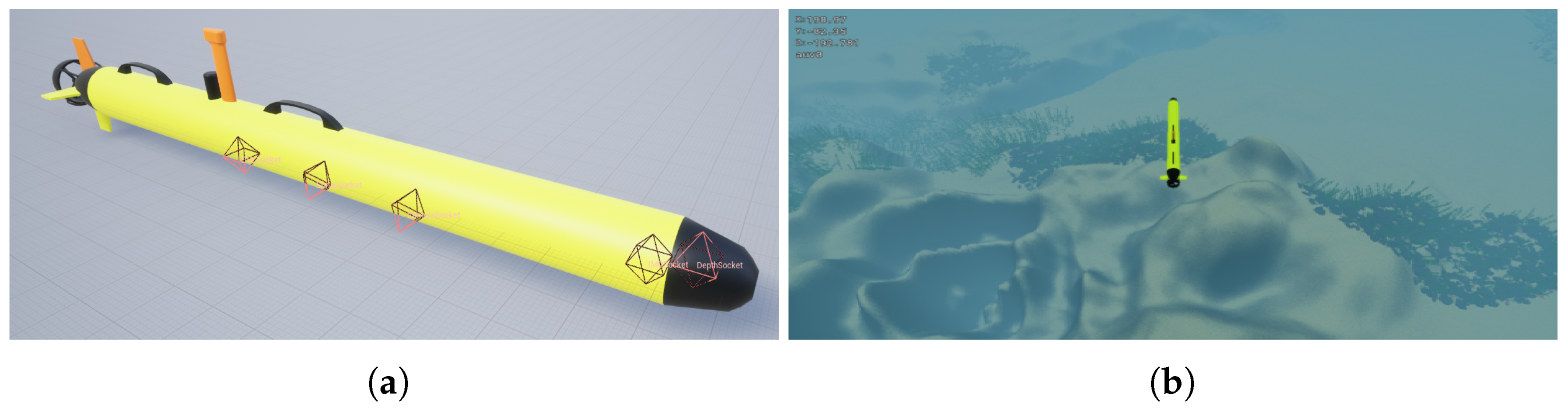
4.2. Simulation

The simulation data employed in this study was generated using HoloOcean 0.5.0 [52,53], a simulation environment built upon Unreal Engine 4. A torpedo-type AUV, equipped with an IMU, DVL, and PS, was employed. The sensor noise characteristics are detailed in

Table 2. Noise statistics for simulation.

Sensor	Noise Type	Noise Standard Bias
IMU	Angular velocity	0.00277 rad/s/Hz
	Linear acceleration	0.00123 m/s2/Hz
	Angular velocity bias	0.00141 rad/s2/Hz
	Linear acceleration bias	0.00388 m/s3/Hz
DVL	Velocity per beam	0.02626 m/s
	Range per beam	0.1 m
PS	Depth sensor	0.255 m

. Specifically, the IMU data were sampled at a frequency of 200 Hz, DVL at 10 Hz, and pressure sensors at 100 Hz, with synchronization performed at the lowest frequency available. The simulated navigator and underwater environment are shown in Figure 2.

The heading and depth adjustments of the navigator are achieved through control of the tail fin angle and thruster parameters. In simulation, four distinct trajectories are employed, and the navigation is conducted within an open water environment. As setup errors were superimposed on the trajectories during the simulation, the treatment of individual trajectories was insufficient to demonstrate the effectiveness of the filter. To address this issue, the algorithm was evaluated using multiple trajectories generated from identical inputs, with consistent propeller and rudder angles. Therefore, by varying the starting point, each trajectory set was subjected to 100 Monte Carlo simulations to eliminate the effects of random errors and biases on the filter.

The simulator delivers highly accurate positional data directly, effectively avoiding the inaccuracies and costs associated with acquiring actual positional data in real-world applications. To replicate real-world conditions, fixed-depth sailing is adopted for data generation. The location and depth of the starting point of each track are $(1.4,-100.5,-151.0)$, $(233.9,41.7,-172.5)$, $(-659.3,-12.4,-126.0)$, and $(158.7209.9,-169.0)$, respectively. A comparative analysis of algorithmic outcomes across diverse trajectories is presented in Figure 3.

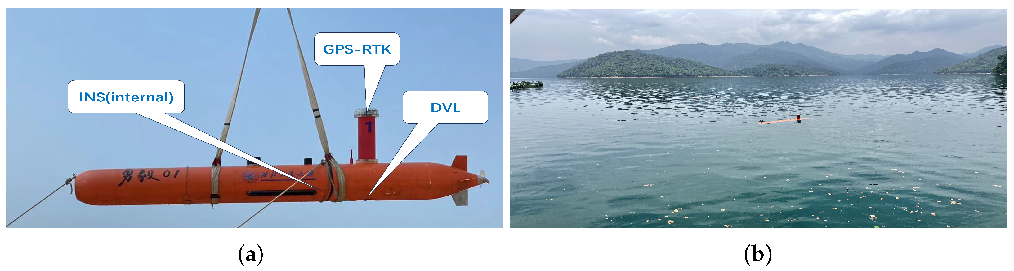
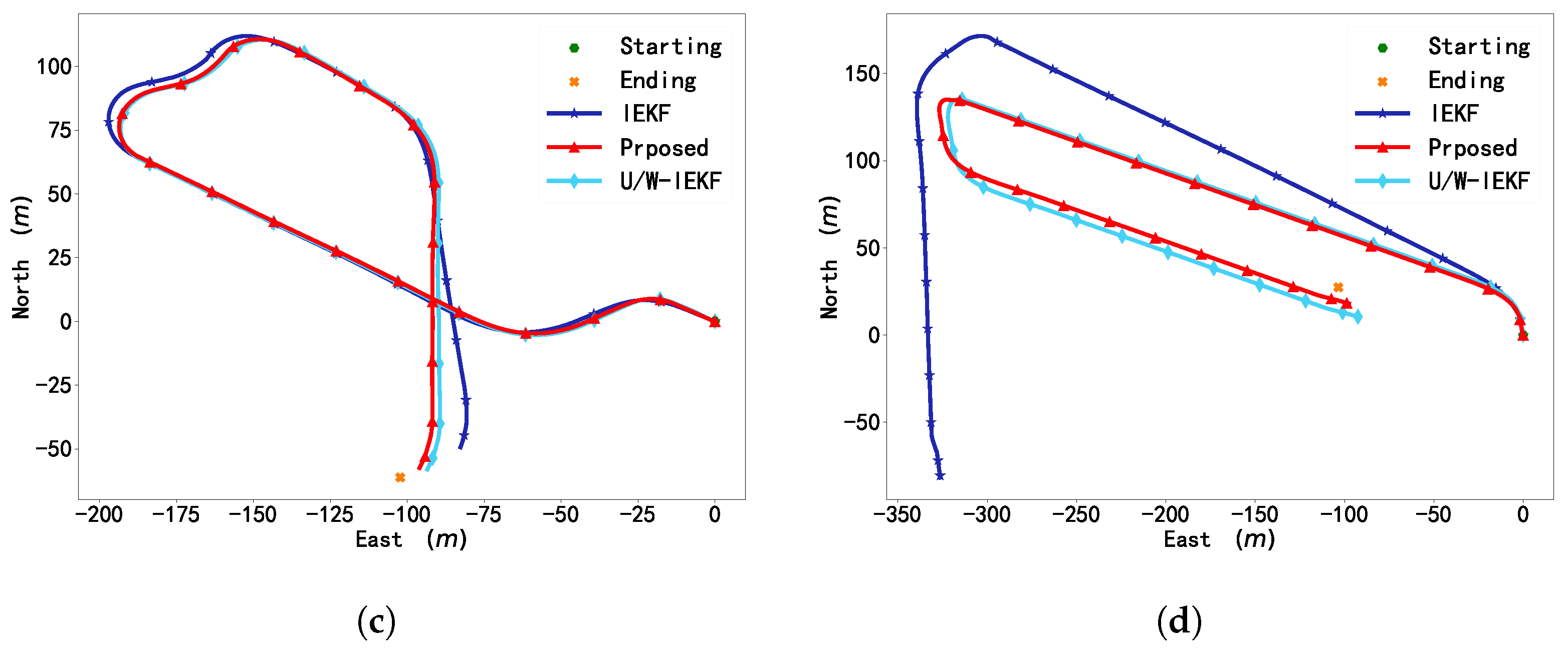
4.3. Natural Scenario Data

The dataset from a previous study [54] is employed in this research to conduct practical validation of the proposed algorithm using data gathered from natural environments. The validation process includes offline computation of global data, followed by comparison with the GNSS positions of the vehicle when it was not submerged in water. It is important to note that the GNSS positions are obtained in differential mode, and any errors associated with them are not considered in this study. Figure 4 illustrates both the vehicle and the acquisition environment employed for data collection. The INS and DVL are equipped with pole arm of dimensions $l=[0,26,9]$ mm. The mounting angle is negligible as it can be pre-measured, thus eliminating its effect. The GPS trajectory differs from the true trajectory only in terms of time delay, and the overall consideration of the trajectory allows the pole arm between the GPS and the body to be ignored.

For the navigator data collected at different latitudes and salinities, the proposed algorithm is used to perform a multi-sensor fusion of waypoint projection. The algorithm is set up with uniform parameters where $Q=diag\left([I_3,I_3,I_3,0.1·I_3,0.001·I_3]\right)$, $Co{v}_{DVL}=0.6·I_3$, $N=diag(Co{v}_{DVL},I_2,0.01)$. The trajectory results are shown in Figure 5. The true position is converted from latitude and longitude to a local position using the European Petroleum Survey Group (EPSG) database [55], starting at $(0,0)$ in meters.

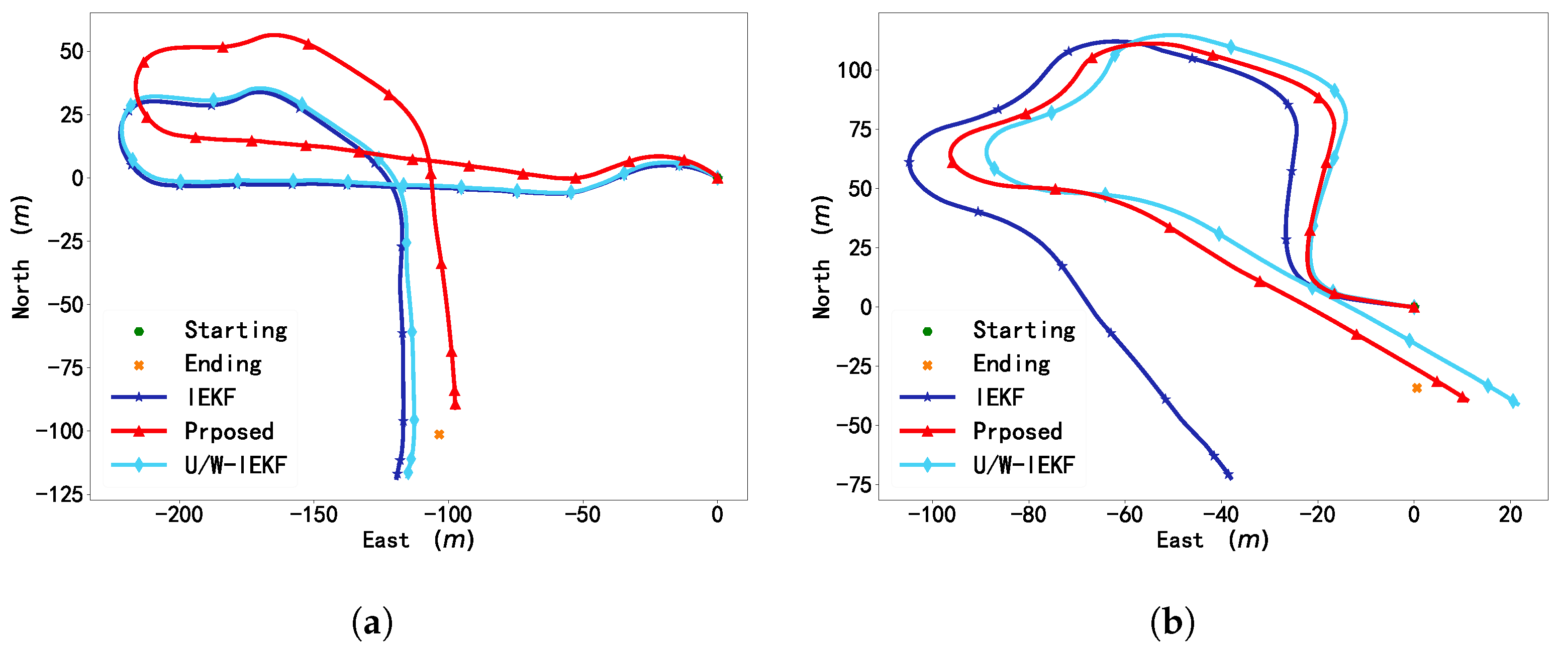
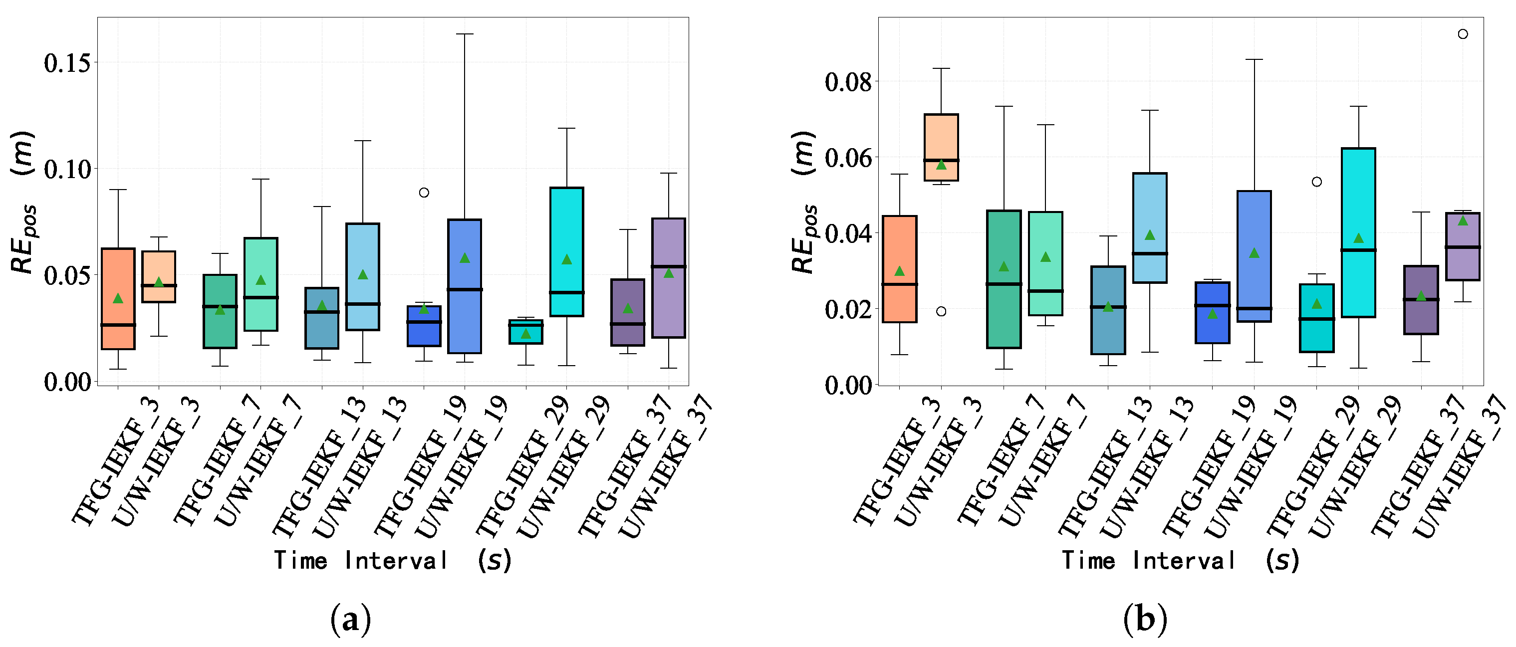
5. Results and Discussion

The comparison of simulation results (Figure 3) reveals that the proposed TFG-IEKF algorithm exhibits superior localization accuracy across various trajectories compared with the underwater IEKF algorithm, which similarly employs Lie group optimization techniques. This superiority can be attributed to the sequential solving of IEKF, where the solving procedure data are conducted only upon input of a particular sensor class, whereas the proposed algorithm optimizes all data types within a uniform framework following frequency synchronization.

The algorithm’s effectiveness is demonstrated by its ability to manage random data errors. We examine the role of the algorithm on trajectory accuracy using RMSE. The results are averaged over multiple times for the same trajectory, and the results are shown in

Table 3. The RMSE of the AUV position and attitude.

Trajectory No.		Traj.1	Traj.2	Traj.3	Traj.4
Position (m)	IEKF	56.5914	69.6770	73.3606	48.9478
	U/W-IEKF	50.8412	93.0147	72.7105	45.4038
	Proposed	11.6488	16.8054	20.5661	9.4366
Attitude (rad)	IEKF	−0.0249	0.0238	−0.0208	0.0082
	U/W-IEKF	0.0136	0.0205	0.0023	−0.0142
	Proposed	−0.0057	0.0074	−0.0066	−0.0013

. The quantitative analysis reveals that the proposed algorithm improves positional accuracy by 77.00% compared with the classical IEKF algorithm and by 57.21% compared with the U/W-IEKF method. It should be noted that the U/W-IEKF method is not stable enough, especially for trajectory 2, resulting in a large error. Excluding trajectory 2, the proposed method shows a 76.01% improvement over the U/W-IEKF method. Regarding attitude accuracy, the proposed method improves by 74.52% over the IEKF method and by 7.32% over the U/W-IEKF method. In conclusion, while the U/W-IEKF method is relatively effective for attitude optimization, the proposed algorithm provides significant improvements in both positional and attitude accuracy.

To assess the robustness of the algorithm throughout the trajectory optimization process, we employ metrics such as Relative Error (RE) [56]. The set $\tilde{S}={\left\{d_k\right\}}_k^K$, $d_k=\{{\widehat{x}}_s,{\widehat{x}}_s\},$ of K pairs of states is chosen from $\widehat{X}$ based on some criteria (e.g., distances along the trajectory). Then RE is denoted by the following:

$$RE=\{\parallel p_e-\Delta R_k{\widehat{p}}_e^{\prime }{{\parallel }_2\}}_{k=1}^{K-1}$$

(47)

where K is the distance or time interval. In this paper, the time step size criterion $K=\{3,7,13,19,29,37\}s$ is selected. The comparison results between the proposed algorithm and the U/W-IEKF method are shown in Figure 6. It can be observed that, although the proposed algorithm exhibits significant uncertainty in the short term, this uncertainty decreases over time and consistently outperforms the U/W-IEKF method.

For real underwater navigation data, the position of AUV upon surfacing and acquiring the Real-Time Kinematic (RTK) signal is regarded as the definitive endpoint. The total navigation error for the entire voyage is computed using the relative metric of horizontal position error (Hori-Error) percentage (PEP) [57] as follows:

$$PEP=\frac{Hori-Error}{D}\times 100\%$$

(48)

where D is the Total Distance Traveled for each trajectory.

We computed the total distance traveled for each trajectory, along with the PEP error at the endpoint. The calculated results are presented in

Table 4. PEP for multiple trajectories in the dataset.

Traj. Seq.	Total Mileage (m)	PEP
		IEKF	U/W-IEKF	Proposed
20210428_1_1	791.4829	0.0247	0.0052	0.0052
20210605_0_0	753.1149	0.0653	0.0208	0.0192
20220718_1_1	409.2852	0.1083	0.1010	0.0148
20220718_2_1	451.1789	0.0307	0.0141	0.0122
20220719_1_2	235.1641	0.0414	0.0249	0.0197
20220816_0_4	1138.8411	0.1127	0.0143	0.0142

. The results demonstrate that the proposed algorithm achieves superior accuracy across most trajectories, with the U/W-IEKF method showing the second-best performance. In certain trajectories, both the proposed algorithm and the U/W-IEKF method yield the same results. Overall, the proposed algorithm enhances accuracy by 77.73% compared with the IEKF method and by 52.69% compared with the U/W-IEKF method.

Based on the results of simulation and dataset optimization, the proposed algorithm exhibits significant benefits in improving the precision of underwater navigation. State updating is achieved by relying on Equations (34)–(36) without the need for auxiliary vectors. Evaluation with the latest U/W-IEKF method demonstrates comparable performance. However, as depicted in Figure 6, the proposed algorithm shows dispersion in positioning accuracy over short time intervals, yet it demonstrates enhanced optimization capability over longer durations. This illustrates the algorithm’s stability throughout the optimization process. Subsequent research efforts will focus on conducting rigorous stability analyses and validation to substantiate the algorithm’s efficacy.

The algorithm presented exhibits improved performance compared with the current underwater Lie groups’ filtering algorithm when tested on actual datasets. However, the algorithm’s performance is constrained in a few trajectories, likely due to interference from water currents or significant inertial misalignments during specific intervals. Notably, the proposed algorithm achieves high accuracy without necessitating intricate transformations. Furthermore, the algorithm demonstrates better outcomes with ideal data (errors following a Gaussian distribution) in comparison with actual navigation data. Nevertheless, the algorithm’s enhanced accuracy across all trajectories highlights its efficacy.

6. Conclusions

This paper addresses the challenge of multi-sensor fusion in underwater navigation by employing Lie group theory for invariant error-based fusion. The proposed algorithm circumvents the necessity of auxiliary vectors, a common limitation in conventional methods to meet group affine constraints, thereby facilitating predictions and updates within both fixed and body frameworks. The algorithm achieves a 77% improvement in accuracy over the standard IEKF and a 52% improvement over U/W-IEKF by incorporating fixed inputs from DVL and depth data through simulations and actual data analyses. Future work will concentrate on enhancing the algorithm’s adaptability to navigators with diverse dynamics and exploring the impact of parameter settings. Similar to AI-IMU research, investigating dynamic parameters through deep learning will be a compelling avenue.

References

1. Yan, J.; Ban, H.; Luo, X.; Zhao, H.; Guan, X. Joint Localization and Tracking Design for AUV with Asynchronous Clocks and State Disturbances. IEEE Trans. Veh. Technol. 2019, 68, 4707–4720. [Google Scholar] [CrossRef]
2. Naus, K.; Piskur, P. Applying the Geodetic Adjustment Method for Positioning in Relation to the Swarm Leader of Underwater Vehicles Based on Course, Speed, and Distance Measurements. Energies 2022, 15, 8472. [Google Scholar] [CrossRef]
3. Huang, H.; Chen, X.; Zhang, B.; Wang, J. High accuracy navigation information estimation for inertial system using the multi-model EKF fusing adams explicit formula applied to underwater gliders. ISA Trans. 2017, 66, 414–424. [Google Scholar] [CrossRef] [PubMed]
4. Kim, T.; Kim, J.; Byun, S.W. A Comparison of Nonlinear Filter Algorithms for Terrain-referenced Underwater Navigation. Int. J. Control Autom. Syst. 2018, 16, 2977–2989. [Google Scholar] [CrossRef]
5. Cheng, C.; Wang, C.; Yang, D.; Liu, W.; Zhang, F. Underwater SLAM Based on Forward-Looking Sonar. In Proceedings of the Cognitive Systems and Signal Processing, Zhuhai, China, 25–27 December 2020; Sun, F., Liu, H., Fang, B., Eds.; Springer: Singapore, 2021; pp. 584–593. [Google Scholar]
6. Bonin-Font, F.; Burguera Burguera, A. NetHALOC: A learned global image descriptor for loop closing in underwater visual SLAM. Expert Syst. 2021, 38, e12635. [Google Scholar] [CrossRef]
7. Liu, R.; Liu, F.; Liu, C.; Zhang, P. Modified Sage-Husa Adaptive Kalman Filter-Based SINS/DVL Integrated Navigation System for AUV. J. Sens. 2021, 2021, 1–8. [Google Scholar] [CrossRef]
8. Pardos, J.; Balaguer, C. RHO humanoid robot bipedal locomotion and navigation using Lie groups and geometric algorithms. In Proceedings of the 2005 IEEE/RSJ International Conference on Intelligent Robots and Systems, Edmonton, AB, Canada, 2–6 August 2005; pp. 3081–3086. [Google Scholar] [CrossRef]
9. Barfoot, T. State Estimation for Robotics; Cambridge University Press: Cambridge, UK, 2017; pp. 1–368. [Google Scholar] [CrossRef]
10. Barrau, A. Non-Linear State Error Based Extended Kalman Filters with Applications to Navigation. (Filtres de Kalman étendus Reposant sur une Variable d’erreur non linéaire Avec Applications à la Navigation). Ph.D. Thesis, Mines Paristech, Paris, France, 2015. [Google Scholar]
11. Barrau, A.; Bonnabel, S. The Invariant Extended Kalman Filter as a Stable Observer. IEEE Trans. Autom. Control 2017, 62, 1797–1812. [Google Scholar] [CrossRef]
12. Hartley, R.; Ghaffari, M.; Eustice, R.M.; Grizzle, J.W. Contact-aided invariant extended Kalman filtering for robot state estimation. Int. J. Robot. Res. 2020, 39, 402–430. [Google Scholar] [CrossRef]
13. Chang, L.; Qin, F.; Xu, J. Strapdown Inertial Navigation System Initial Alignment Based on Group of Double Direct Spatial Isometries. IEEE Sens. J. 2022, 22, 803–818. [Google Scholar] [CrossRef]
14. Barrau, A.; Bonnabel, S. A Mathematical Framework for IMU Error Propagation with Applications to Preintegration. In Proceedings of the 2020 IEEE International Conference on Robotics and Automation (ICRA), Paris, France, 31 May–31 August 2020; pp. 5732–5738. [Google Scholar] [CrossRef]
15. Brossard, M.; Barrau, A.; Chauchat, P.; Bonnabel, S. Associating Uncertainty to Extended Poses for on Lie Group IMU Preintegration with Rotating Earth. IEEE Trans. Robot. 2022, 38, 998–1015. [Google Scholar] [CrossRef]
16. Tang, H.; Xu, J.; Chang, L.; Shi, W.; He, H. Invariant Error-Based Integrated Solution for SINS/DVL in Earth Frame: Extension and Comparison. IEEE Trans. Instrum. Meas. 2023, 72, 9500617. [Google Scholar] [CrossRef]
17. Barrau, A.; Bonnabel, S. The Geometry of Navigation Problems. IEEE Trans. Autom. Control 2023, 68, 689–704. [Google Scholar] [CrossRef]
18. Shi, W.; Xu, J.; Li, D.; He, H. Attitude Estimation of SINS on Underwater Dynamic Base with Variational Bayesian Robust Adaptive Kalman Filter. IEEE Sens. J. 2022, 22, 10954–10964. [Google Scholar] [CrossRef]
19. Jørgensen, E.K.; Fossen, T.I.; Bryne, T.H.; Schjølberg, I. Underwater Position and Attitude Estimation Using Acoustic, Inertial, and Depth Measurements. IEEE J. Ocean. Eng. 2020, 45, 1450–1465. [Google Scholar] [CrossRef]
20. Li, P.; Liu, Y.; Yan, T.; Yang, S.; Li, R. A Robust INS/USBL/DVL Integrated Navigation Algorithm Using Graph Optimization. Sensors 2023, 23, 916. [Google Scholar] [CrossRef] [PubMed]
21. Huang, H.; Tang, J.; Zhang, B. Positioning Parameter Determination Based on Statistical Regression Applied to Autonomous Underwater Vehicle. Appl. Sci. 2021, 11, 7777. [Google Scholar] [CrossRef]
22. OuYang, M.; Fan, H.; Du, P. Particle Swarm Optimization for Underwater Gravity-Matching: Applications in Navigation and Simulation. Int. Arch. Photogramm. Remote Sens. Spat. Inf. Sci. 2022, XLVI-3/W1-2022, 149–154. [Google Scholar] [CrossRef]
23. Jin, K.; Chai, H.; Su, C.; Xiang, M.; Hui, J. An optimization-based in-motion fine alignment and positioning algorithm for underwater vehicles. Measurement 2022, 202, 111746. [Google Scholar] [CrossRef]
24. Russo, P.; Di Ciaccio, F.; Troisi, S. DANAE++: A Smart Approach for Denoising Underwater Attitude Estimation. Sensors 2021, 21, 1526. [Google Scholar] [CrossRef]
25. Zhang, D.; Chang, S.; Zou, G.; Wan, C.; Li, H. A Robust Graph-Based Bathymetric Simultaneous Localization and Mapping Approach for AUVs. IEEE J. Ocean. Eng. 2024, 49, 1–21. [Google Scholar] [CrossRef]
26. Rahman, S.; Li, A.Q.; Rekleitis, I. SVIn2: An Underwater SLAM System using Sonar, Visual, Inertial, and Depth Sensor. In Proceedings of the 2019 IEEE/RSJ International Conference on Intelligent Robots and Systems (IROS), Macau, China, 3–8 November 2019; pp. 1861–1868. [Google Scholar] [CrossRef]
27. Ma, H.; Mu, X.; He, B. Adaptive Navigation Algorithm with Deep Learning for Autonomous Underwater Vehicle. Sensors 2021, 21, 6406. [Google Scholar] [CrossRef] [PubMed]
28. He, Q.; Yu, H.; Fang, Y. NINT: Neural Inertial Navigation Based on Time Interval Information in Underwater Environments. IEEE Sens. J. 2024, 24, 21719. [Google Scholar] [CrossRef]
29. Li, D.; Xu, J.; He, H.; Wu, M. An Underwater Integrated Navigation Algorithm to Deal With DVL Malfunctions Based on Deep Learning. IEEE Access 2021, 9, 82010–82020. [Google Scholar] [CrossRef]
30. Zhao, W.; Zhao, S.; Zhang, G.; Liu, G.; Meng, W. FL-EKF Based Cooperative Localization Method for Multi-AUVs. IEEE Internet Things J. 2024, 11, 1–12. [Google Scholar] [CrossRef]
31. Qin, J.; Li, M.; Li, D.; Zhong, J.; Yang, K. A Survey on Visual Navigation and Positioning for Autonomous UUVs. Remote Sens. 2022, 14, 3794. [Google Scholar] [CrossRef]
32. Kim, B.; Joe, H.; Yu, S.C. High-precision Underwater 3D Mapping Using Imaging Sonar for Navigation of Autonomous Underwater Vehicle. Int. J. Control Autom. Syst. 2021, 19, 3794. [Google Scholar] [CrossRef]
33. Costanzi, R.; Fanelli, F.; Monni, N.; Ridolfi, A.; Allotta, B. An Attitude Estimation Algorithm for Mobile Robots under Unknown Magnetic Disturbances. IEEE/ASME Trans. Mechatron. 2016, 21, 1900–1911. [Google Scholar] [CrossRef]
34. Ngatini; Apriliani, E.; Nurhadi, H. Ensemble and Fuzzy Kalman Filter for position estimation of an autonomous underwater vehicle based on dynamical system of AUV motion. Expert Syst. Appl. 2017, 68, 29–35. [Google Scholar] [CrossRef]
35. Shariati, H.; Moosavi, H.; Danesh, M. Application of particle filter combined with extended Kalman filter in model identification of an autonomous underwater vehicle based on experimental data. Appl. Ocean. Res. 2019, 82, 32–40. [Google Scholar] [CrossRef]
36. Pei, F.; Xu, H.; Jiang, N.; Zhu, D. A novel in-motion alignment method for underwater SINS using a state-dependent Lie group filter. Navigation 2020, 67, 451–470. [Google Scholar] [CrossRef]
37. Xu, C.; Xu, C.; Wu, C.; Qu, D.; Liu, J.; Wang, Y.; Shao, G. A novel self-adapting filter based navigation algorithm for autonomous underwater vehicles. Ocean. Eng. 2019, 187, 106146. [Google Scholar] [CrossRef]
38. Fossen, T.I. Feedback error-state Kalman filter with time-delay compensation for hydroacoustic-aided inertial navigation of underwater vehicles. Control. Eng. Pract. 2023, 138, 105603. [Google Scholar] [CrossRef]
39. Barrau, A.; Bonnabel, S. Invariant Kalman Filtering. Annu. Rev. Control Robot. Auton. Syst. 2018, 1, 237–257. [Google Scholar] [CrossRef]
40. Chang, L.; Luo, Y. Log-Linear Error State Model Derivation without Approximation for INS. IEEE Trans. Aerosp. Electron. Syst. 2023, 59, 2029–2035. [Google Scholar] [CrossRef]
41. Li, J.; Zhang, S.; Yang, H.; Jiang, Z.; Bai, X. A Fast Continuous Self-Calibration Method for FOG Rotational Inertial Navigation System Based on Invariant Extended Kalman Filter. IEEE Sens. J. 2023, 23, 2456–2469. [Google Scholar] [CrossRef]
42. Barfoot, T.D.; Furgale, P.T. Associating Uncertainty with Three-Dimensional Poses for Use in Estimation Problems. IEEE Trans. Robot. 2014, 30, 679–693. [Google Scholar] [CrossRef]
43. Roux, A.; Changey, S.; Weber, J.; Lauffenburger, J.P. CNN-based Invariant Extended Kalman Filter for projectile trajectory estimation using IMU only. In Proceedings of the 2021 International Conference on Control, Automation and Diagnosis (ICCAD), Grenoble, France, 3–5 November 2021; pp. 1–6. [Google Scholar] [CrossRef]
44. Chang, L.; Di, J.; Qin, F. Inertial-Based Integration With Transformed INS Mechanization in Earth Frame. IEEE/ASME Trans. Mechatron. 2022, 27, 1738–1749. [Google Scholar] [CrossRef]
45. Xu, B.; Guo, Y. A Novel DVL Calibration Method Based on Robust Invariant Extended Kalman Filter. IEEE Trans. Veh. Technol. 2022, 71, 9422–9434. [Google Scholar] [CrossRef]
46. Luo, L.; Huang, Y.; Zhang, Z.; Zhang, Y. A New Kalman Filter-Based In-Motion Initial Alignment Method for DVL-Aided Low-Cost SINS. IEEE Trans. Veh. Technol. 2021, 70, 331–343. [Google Scholar] [CrossRef]
47. Qian, L.; Qin, F.; Li, K.; Zhu, T. Research on the Necessity of Lie Group Strapdown Inertial Integrated Navigation Error Model Based on Euler Angle. Sensors 2022, 22, 7742. [Google Scholar] [CrossRef]
48. Potokar, E.R.; Norman, K.; Mangelson, J.G. Invariant Extended Kalman Filtering for Underwater Navigation. IEEE Robot. Autom. Lett. 2021, 6, 5792–5799. [Google Scholar] [CrossRef]
49. Luo, Y.; Lu, F.; Guo, C.; Liu, J. Matrix Lie Group-Based Extended Kalman Filtering for Inertial-Integrated Navigation in the Navigation Frame. IEEE Trans. Instrum. Meas. 2024, 73, 9503916. [Google Scholar] [CrossRef]
50. Luo, Y.; Wang, M.; Guo, C. The Geometry and Kinematics of the Matrix Lie Group SE_K(3). arXiv 2020, arXiv:2012.00950. [Google Scholar]
51. Ashkenazi, V. Coordinate Systems: How to Get Your Position Very Precise and Completely Wrong. J. Navig. 1986, 39, 269–278. [Google Scholar] [CrossRef]
52. Potokar, E.; Lay, K.; Norman, K.; Benham, D.; Neilsen, T.B.; Kaess, M.; Mangelson, J.G. HoloOcean: Realistic Sonar Simulation. In Proceedings of the 2022 IEEE/RSJ International Conference on Intelligent Robots and Systems (IROS), Kyoto, Japan, 23–27 October 2022; pp. 8450–8456. [Google Scholar] [CrossRef]
53. Potokar, E.; Ashford, S.; Kaess, M.; Mangelson, J.G. HoloOcean: An Underwater Robotics Simulator. In Proceedings of the 2022 International Conference on Robotics and Automation (ICRA), Yokohama, Japan, 13–17 May 2022; pp. 3040–3046. [Google Scholar] [CrossRef]
54. Wang, C.; Cheng, C.; Yang, D.; Pan, G.; Zhang, F. Underwater AUV Navigation Dataset in Natural Scenarios. Electronics 2023, 12, 3788. [Google Scholar] [CrossRef]
55. Nicolai, R.; Simensen, G. The New EPSG Geodetic Parameter Registry. In Proceedings of the 70th EAGE Conference and Exhibition incorporating SPE EUROPEC 2008, Rome, Italy, 9–12 June 2008. [Google Scholar] [CrossRef]
56. Zhang, Z.; Scaramuzza, D. A Tutorial on Quantitative Trajectory Evaluation for Visual(-Inertial) Odometry. In Proceedings of the 2018 IEEE/RSJ International Conference on Intelligent Robots and Systems (IROS), Madrid, Spain, 1–5 October 2018; pp. 7244–7251. [Google Scholar] [CrossRef]
57. Tang, J.; Bian, H.; Ma, H.; Wang, R. Initialization of SINS/GNSS Error Covariance Matrix Based on Error States Correlation. IEEE Access 2023, 11, 94911–94917. [Google Scholar] [CrossRef]
Figure 1. AUV is localized by multi-source data from underwater TFG-IEKF.
Jmse 12 01178 g001
Figure 2. HoloOcean simulation environment and vehicles, where (a) is the simulation environment of HoloOcean in open water, and (b) is the slewing body-type vehicle in HoloOcean [53].
Jmse 12 01178 g002
Figure 3. Comparison of localization results for four sets of trajectories in the simulation environment. The original data represent the online data after INS/DVL fusion by the AUV in a specific way (integrated within the Inertial Unit), with (a) trajectory 1, (b) trajectory 2, (c) trajectory 3, and (d) trajectory 4.
Jmse 12 01178 g003
Figure 4. Vehicle used for data acquisition and data acquisition environment, where (a) shows the AUV for data acquisition in a lake, and (b) shows the data acquisition in a marine environment.
Jmse 12 01178 g004
Figure 5. Comparison of REs between the proposed algorithm and the state-of-the-art Underwater IEKF method for each set of trajectories at different time scales. with (a) scenario 1, (b) scenario 2, (c) scenario 3, and (d) scenario 4.
Jmse 12 01178 g005aJmse 12 01178 g005b
Figure 6. Various types of AUV tracks in different regions, with (a) RE of Traj. 1, (b) RE of Traj. 2, (c) RE of Traj. 3, and (d) RE of Traj. 4. In the figure, circles indicate outliers, triangles indicate means, and the horizontal line in the box indicates the median.
Jmse 12 01178 g006aJmse 12 01178 g006b