The Effect of Model Input Uncertainty on the Simulation of Typical Pollutant Transport in the Coastal Waters of China

Abstract

Route planning to evade potential pollution holds critical importance for aquaculture vessels. This study establishes a fish-feed pollutant drift model based on the Lagrangian particle tracking algorithm and designs four sets of sensitivity experiments in the East China Sea. The research investigates the impact of model input uncertainties on the drift trajectory, centroid position, and sweeping area of the fish-feed pollutants. Numerical results indicate that the uncertainty in the background flow field significantly affects the uncertainty in the centroid position and sweeping area in the numerical simulations. Specifically, when a 35% random error is added to the background flow field, the centroid shift distance reaches its maximum, and the sweeping area also attains its largest value. The uncertainty in the background wind field affects the centroid position of particles but to a much lesser extent compared to the background flow field. When considering only the uncertainty of the background wind field, the sweeping area does not significantly differ from the control experiment as the uncertainty of the background wind field increases. The initial release position has little effect on the drift direction of the fish-feed pollutants but does affect the drift distance; it has minimal impact on the trajectory but significantly affects the final position of the pollutant centroid. By analyzing the model uncertainties, this study reveals the key factors influencing the drift of fish-feed pollutants. This information is crucial for aquaculture vessels in planning routes, considering environmental factors, and reducing potential pollution risks.

1. Introduction

Currently, China has become one of the largest consumers of seafood in the world [1]. Traditional nearshore cage aquaculture is vulnerable to natural disasters such as typhoons and red tides. Additionally, the limited spatial resources nearshore, high farming densities, and susceptibility to disease outbreaks significantly impact the productivity of aquaculture [2,3]. In order to mitigate the impact of natural disasters and enhance fish production, a novel approach to offshore aquaculture has emerged in recent years known as an enclosed aquaculture vessel. It holds promise as a significant avenue for the development of offshore aquaculture [4,5]. Currently, enclosed aquaculture vessels are being utilized in countries such as China, Japan, South Korea, Norway, and Scotland [6,7,8,9]. In 2022, China launched and commissioned the Conson No 1, the world’s first 100,000-metric ton intelligent-fishery large-scale aquaculture vessel.

The aquaculture tanks on enclosed aquaculture vessels are relatively enclosed structures that undergo continuous water circulation 24 h a day. This ensures that high-density fish populations are consistently maintained in an optimal marine environment [10]. However, the excrement produced by the farmed fish after consuming feed and the residual feed after feeding is discharged into the seawater through the circulating water exchange system. Pollutants are transported in seawater by flow and wind fields. To prevent long-term discharge and accumulation of pollutants, which can lead to localized water pollution, and to provide a more suitable environment for the farmed fish, the enclosed aquaculture vessel periodically changes its farming location. Due to the presence of the water circulation system, the next location should be chosen to avoid areas with pollutants.

The fate of feed pollutants in the ocean is difficult to observe directly, making the use of models to simulate the transport and impact of these pollutants particularly important. Enclosed aquaculture vessels, used as a novel offshore aquaculture approach developed in recent years, have limited research available on the transport of fish-feed pollutants. Previous studies on the transport of other marine pollutants such as spilled oil and microplastics have primarily used Eulerian methods, Lagrangian methods, and Eulerian–Lagrangian methods [11,12]. Wang et al. used the Lagrangian method to develop a drift model for fish-feed pollutants, deriving empirical formulas to describe pollutant distribution and providing reasonable planning for the route design of the enclosed aquaculture vessels [13]. However, due to inherent errors in numerical simulations and uncertainties in background flow fields and wind fields [14], numerical experiments may sometimes fail to provide perfect simulation and prediction results [15].

To ensure the reliability of numerical simulations and the accuracy of model predictions, it is necessary to analyze the uncertainty of the model [16]. Elliott and Jones pointed out that in simulating the transport of oil pollutants, the effect of wind is significantly greater than that of ocean currents [17]. Gonçalves et al. developed an uncertainty quantification framework for deep-sea oil models and found that uncertain inputs are primarily generated by ocean currents [18]. Jorda et al.’s research revealed that errors in background wind and flow fields have a significant impact on the final outputs of oil spill simulations, which cannot be overlooked [15]. Browne et al. found that the number of microplastic particles in downstream estuarine locations is typically more than three times higher than in upwind locations, indicating the crucial role of wind in the distribution of microplastic particles [19]. Extensive studies by numerous scholars have demonstrated that ocean currents, Stokes drift, Ekman drift, river plumes, and coastal currents are key factors determining the transport of microplastics [20,21,22,23]. Van Sebille et al. provided a comprehensive overview of the physical mechanisms governing the transport of microplastics [20]. They found that different oceanic regions exhibit distinct flow characteristics, which can result in varying influences on the drift of microplastics. Moreover, the uncertainty associated with ocean currents affects both the drift and fate of microplastics, highlighting the need for in-depth research in this area.

Previous research on traditional pollutants has provided valuable insights for our study. When investigating feed pollutants, uncertainties in factors such as background flow fields, background wind fields, and initial particle-release positions can influence the transport and fate of the pollutants in the ocean. In this study, we established a drift model for feed pollutants based on the Lagrangian method and conducted a series of experiments to investigate the impact of uncertainties in ocean currents, wind, and initial release positions on the simulation results. The first set of experiments introduced artificial random perturbations into the ocean currents to study the influence of uncertainty in ocean currents on the simulation results. The second set of experiments introduced artificial random perturbations into the wind to study the influence of uncertainty in wind on the simulation results. The third set of experiments examined the impact of different initial release positions on the simulation results. This study aims to provide insights into the rational planning of navigation routes for future aquaculture vessels.

2. Model and Methodology

2.1. Model Description

Once introduced into the ocean, feed pollutants are primarily influenced by convective diffusion. The governing equation is shown as Equation (1):

$${\displaystyle \frac{\partial C}{\partial t}}+\overrightarrow{V}\cdot \nabla C=\nabla \cdot \left(\overrightarrow{D}\cdot \nabla C\right)$$

(1)

In Equation (1), $\nabla$ is the gradient operator, C is the concentration of feed pollutants in seawater, and $\overrightarrow{V}$ is the convective velocity vector. $\overrightarrow{D}\left(D_x,D_y,D_z\right)$ is the isotropic diffusion coefficient in the horizontal direction, where $D_x$, $D_y$, and $D_z$ are the diffusion coefficients in the $x$, $y$, and $z$ directions, respectively (m²/s). Since $\overrightarrow{D}$ is isotropic in the horizontal direction, $D_x$ and $D_y$ are collectively referred to as the horizontal diffusion coefficient $D_h$, such that $D_x=D_y=D_h$.

To accurately simulate various processes, it is essential to employ suitable numerical techniques, including the finite difference method, finite element method, or finite volume method, for solving the convection–diffusion Equation (1) [24,25]. In this study, the Lagrangian particle tracking method is employed. Feed pollutants are discretized into a certain number of particles, where each serves as a representative for a cluster of feed pollutants characterized by size, velocity, and spatial coordinates. After these particles are released at a specific location in the seawater, they move under the influence of flow, turbulence, and buoyancy. The characteristics of the feed pollutants (density and particle size) are integrated into each particle as model inputs. These particles are subsequently utilized to ascertain whether they float or sink in the sea water. The diffusion process induced by ocean turbulence, being stochastic, is simulated using random motion, while the advection process of the particles is primarily controlled by deterministic methods considering environmental dynamic processes such as ocean currents and wind. By conducting a statistical analysis of the positions of all the particles, we can accurately determine the spatiotemporal distribution of feed pollutants within the marine environment.

When using the Lagrangian particle-tracking algorithm to simulate the transport of feed pollutants, the three-dimensional motion of the feed pollutant particles is described as follows:

$${\displaystyle \frac{d\overrightarrow{S}}{dt}}={\overrightarrow{U}}_c+{\overrightarrow{U}}_d+\alpha E{\overrightarrow{U}}_w+U_s\overrightarrow{k}$$

(2)

Here, $\overrightarrow{S}=\left(x,y,z\right)$ is the displacement vector of a feed-pollutant particle, and $x$, $y$, and $z$ are the Cartesian coordinates. ${\overrightarrow{U}}_c\left(u_{cx}\overrightarrow{i},v_{cy}\overrightarrow{j},u_{cz}\overrightarrow{k}\right)$ and ${\overrightarrow{U}}_d\left(u^{\prime }\overrightarrow{i},v^{\prime }\overrightarrow{j},w^{\prime }\overrightarrow{k}\right)$ are the velocity of the ocean current and the diffusion velocity in the turbulent diffusion process, respectively. $U_s$ is the settling velocity, and $\overrightarrow{k}$ is the unit vector in the vertical direction. The expression for $U_s$ is shown in Equations (3) and (4) [26,27]:

$$U_s=\{\begin{array}{cc}{U}_{s,S}& \begin{array}{c}{Re}_p<0.2\end{array}\\ U_{s,S}{\left(1+0.15{Re}_p^{0.687}\right)}^{-1}& \begin{array}{cc}& 0.2<{Re}_p<750\end{array}\end{array}$$

(3)

$$U_{s,S}={\displaystyle \frac{\left({\rho }_w-{\rho }_f\right)g{d}^2}{18{\mu }_w}}$$

(4)

where $R{e}_p=U_s{\rho }_{w}d/{\mu }_w$ is the particle Reynolds number, and ${\rho }_w$ and ${\rho }_f$ are the densities of seawater (1024 kg/m³) and fish feed (500 kg/m³), respectively. d is the diameter of the feed-pollutant particles. ${\mu }_w$ is the dynamic viscosity of seawater (1.01 × 10⁻³ Pa·s). When $U_s\ge 0$, the particles float or remain suspended in the water, and when $U_s<0$, the particles sink. It is worth noting that according to Waldschläger and Schüttrumpf (2019) [28], the determination of sinking and rising velocities should consider different drag coefficients based on the specific conditions and properties of the particles. The present parametrization may overlook the more complex relationship between particle shape, drag coefficient, and velocity.

The $\alpha E{\overrightarrow{U}}_w$ in Equation (2) represents the wind-stress effect, in which $\alpha =0.03$ is the wind-stress coefficient. It is worth mentioning that the wind-stress coefficient necessitates refinement through additional observational data. Presently, a reference value ($\alpha =0.03$) is being utilized, which aligns with the conventionally adopted coefficient for estimating the wind-driven transport of oil pollutants [14,29]. ${\overrightarrow{U}}_w\left(u_{wx}\overrightarrow{i},u_{wy}\overrightarrow{j}\right)$ is the wind vector at 10 m above the sea surface. $E$ is a transform matrix that represents the velocity caused by wind drag under different wind speeds and is employed in the calculation of the wind deflection angle $\gamma$ [30].

$$E=\left[\begin{array}{cc}\cos \gamma & \sin \gamma \\ -\sin \gamma & \cos \gamma \end{array}\right]$$

(5)

In Equation (5), when $\left|{\overrightarrow{U}}_w\right|\le 25 \mathrm{m}/\mathrm{s}$, $\gamma ={40}^{\circ }-8\sqrt{\left|{\overrightarrow{U}}_w\right|}$, and when $\left|{\overrightarrow{U}}_w\right|>25 \mathrm{m}/\mathrm{s}$, $\gamma =0$ [31].

The diffusion velocity ${\overrightarrow{U}}_d\left(u^{\prime }\overrightarrow{i},v^{\prime }\overrightarrow{j},w^{\prime }\overrightarrow{k}\right)$ in Equation (2) is treated as a random variable, and its components are calculated using the random walk method as follows:

$$(u’,v’,w’)=\sqrt{{\displaystyle \frac{6}{\Delta t}}}\left(R_x\sqrt{D_h},R_y\sqrt{D_h},R_z\sqrt{D_z}\right)$$

(6)

where $\Delta t$ is the time step. $R_x$, $R_y$, and $R_z$ are independent of each other and are assumed to be uniformly distributed random numbers ranging from −1 to 1. $D_h$ is the horizontal diffusion coefficient, calculated using the functional form proposed by Pan et al. as follows [32]:

$$D_h=0.027t^{1.34}$$

(7)

The vertical turbulent diffusion coefficient $D_z$ is calculated following the study of Boufadel et al. [33]:

$$D_z=\left({\displaystyle \frac{\kappa u_{*}}{0.9}}\theta \right)\left(z+z_0\right)\left(1-{\displaystyle \frac{z}{MLD}}\right)$$

(8)

where $\kappa =0.4$ is the von Karman constant, $u_{*}$ is the water friction velocity, and $\theta$ is the “enhancement factor” associated with Langmuir circulation, set to 1.0 in this study. MLD is the mixed layer depth, defined in the current study as the depth where the temperature is 0.2 °C lower than the sea surface temperature. The vertical coordinate system is defined with z = 0 representing the mean sea level. Negative z values indicate positions below the mean sea level. When $z=0$, the vertical turbulent diffusion coefficient $D_z$ is set to $D_z\left(z=0\right)=\left({\displaystyle \frac{\kappa u_{*}}{0.9}}\theta \right)$. The roughness length, denoted by $z_0$, serves as an indicator of the surface roughness resulting from the influence of regular waves. Its calculation is outlined as follows:

$$z_0=1.38\times {10}^{-4}{H}_s{\left(U_w/c_p\right)}^{2.66}$$

(9)

Here, $H_s$ is the significant wave height, and $c_p$ is the wave phase velocity, which is related to the wave period $T$ and is expressed as $c_p={\displaystyle \frac{gT}{2\pi }}$.

The friction velocity $u_{*}$ in Equation (5) can be calculated as [34]:

$$u_{*}=\{\begin{array}{cc}\sqrt{{\rho }_a{C}_{d1}{U}_w\left(U_w-U_{sur}\right)/{\rho }_w}\hfill & \hfill z=0\\ \sqrt{{\rho }_a/{\rho }_w}\kappa U_w/\ln \left(10/z_0\right)\hfill & \hfill z\ne -H \& z\ne 0\\ \sqrt{C_{d2}{U}_{bot}/{\rho }_w}\hfill & \hfill z=-H\end{array}$$

(10)

Here, $U_{sur}$ is the surface current velocity, $U_{bot}$ is the bottom current velocity, ${\rho }_w$ represents the water density, and ${\rho }_a$ represents the air density. $C_{d1}=1.13\times {10}^{-3}$ is the drag coefficient at the sea surface, and $C_{d2}$ is the drag coefficient at the seabed, which is computed by matching with a logarithmic boundary layer at height $z_{ab}$ above the seabed [14].

$$C_{d2}=\max \left[{\displaystyle \frac{{\kappa }^2}{\ln \left(\frac{z_{ab}}{z_0}\right)}},0.0025\right]$$

(11)

2.2. Experimental Design

The Regional Ocean Modeling System (ROMS) is a versatile, open-source, three-dimensional ocean model that is extensively utilized for simulating diverse oceanic motions, spanning from global-scale ocean circulations to intricate water movements within rivers and channels. Furthermore, it serves as a pivotal tool for conducting research across various disciplines, encompassing air–sea interactions, marine biology, marine geology, and the study of sea ice. The ROMS, which has undergone rigorous validation in previous studies [35,36,37], serves as the foundation for generating the velocity, temperature, and salinity data utilized in this research [38,39]. The study area is illustrated in Figure 1, and for detailed ROMS model settings, please refer to [13].

The dynamic boundary condition of the ROMS at the sea surface $z=\zeta (x,y,t)$ is given by:

$$\begin{array}{l}v{\displaystyle \frac{\partial u}{\partial z}}={\tau }_s^x\left(x,y,t\right)\\ v{\displaystyle \frac{\partial v}{\partial z}}={\tau }_s^y\left(x,y,t\right)\end{array}$$

(12)

The thermodynamic boundary condition is:

$$\begin{array}{l}{\kappa }_T{\displaystyle \frac{\partial T}{\partial z}}={\displaystyle \frac{Q_T}{{\rho }_0{c}_p}}+{\displaystyle \frac{1}{{\rho }_0{c}_p}}{\displaystyle \frac{d{Q}_T}{dT}}\left(T-T_{ref}\right)\\ {\kappa }_S{\displaystyle \frac{\partial S}{\partial z}}={\displaystyle \frac{\left(E-P\right)S}{{\rho }_0}}\end{array}$$

(13)

The boundary condition for vertical motion at the sea surface is:

$$w={\displaystyle \frac{\partial \zeta }{\partial t}}$$

(14)

The dynamic boundary condition at the seabed at depth $z=-h\left(x,y\right)$ is:

$$\begin{array}{l}v{\displaystyle \frac{\partial u}{\partial z}}={\tau }_b^x\left(x,y,t\right)\\ v{\displaystyle \frac{\partial v}{\partial z}}={\tau }_b^y\left(x,y,t\right)\end{array}$$

(15)

The thermodynamic boundary condition is:

$$\begin{array}{l}{\kappa }_T{\displaystyle \frac{\partial T}{\partial z}}=0\\ {\kappa }_S{\displaystyle \frac{\partial S}{\partial z}}=0\end{array}$$

(16)

The boundary condition for vertical motion at the sea surface is:

$$-w+\overrightarrow{v}\cdot \nabla h=0$$

(17)

In Equations (12)–(17), ${\tau }_S^x$ and ${\tau }_S^y$ represent the wind stress at the sea surface, $Q_T$ is the heat flux at the sea surface, $E-P$ denotes the freshwater flux, and $T_{ref}$ is the reference temperature at the sea surface.

The tidal forces at the open boundaries were determined using the TPXO.7.0 global inverse tide model developed by Oregon State University (OSU) [36,40]. The tidal heights are composed of four tidal constituents: M₂, S₂, K₁, and O₁, which explain 90% of the tidal variations in the region. The harmonic constants for each constituent were obtained through linear interpolation of the OSU global tidal model. The open boundary conditions for the barotropic component include the Chapman condition for the surface elevation and the Flather condition for the barotropic velocity [41,42]. The open boundary conditions for the baroclinic component are specified using Orlanski-type radiation conditions [43].

To investigate the impact of uncertainties in the background wind and flow fields, as well as the differences in initial release positions on the transport of pollutants generated from fish-feed discharge in seawater, three sets of numerical experiments were designed. Experiment 1 served as the control experiment. As shown in Figure 1, Experiment 1 selects the location K0 (122.5° E, 27° N), represented by the red pentagon, as the initial release position for the particles. The model start time is set to 16 April 2021, with a duration of 360 h. The model simulates the transport of pollutants using 100,000 Lagrangian particles after discharge into the sea. It is worth mentioning that the fish-feed density can differ significantly based on its specific composition and formulation. Common types of fish feed, such as pellets or flakes, typically have densities ranging from approximately 267.11 to 711.35 kg/m³ and particle sizes of about 1 to 8 mm [44]. In this study, due to the difficulty of directly observing certain parameters of fish feed, such as diameter and density, we make several assumptions. For the diameter distribution, we assume a normal distribution centered at 4.5 µm with a standard deviation of 1 µm. With regard to density, we assign a value of 5 × 10² kg/m³. Model parameters can be found in

Table 1. Model settings.

Model Parameters	Value
Release depth	0 m
Release duration	15 days
Simulation duration	15 days
Particle quantity	100,000
Particle density	500 kg/m3

.

Generally, for China’s offshore wave forecast, the mean relative error (MRE) in wave height is about 30%, and the mean absolute error (MAE) is less than 0.5 m. Furthermore, for the wavelength forecast, the MRE is generally less than 30%, and the MAE is generally less than 5 m. At present, the wind speed forecast error of wind farms in China is about 25–40% [45]. Therefore, we choose 35% as the maximum random error added.

In the first set of numerical experiments, the background wind field and the initial release position remain unchanged, using the same data as in Experiment 1. We introduce artificial random perturbations to the background flow field by adding 5%, 15%, 25%, and 35% random errors to the background flow field from Experiment 1 in Experiments 2, 3, 4, and 5, respectively. The method for introducing artificial random perturbations to the background flow field is shown in Equation (18) [46]:

$$\{\begin{array}{c}u=\left[\left(2r-1\right)\times e+1\right]\times u_0\\ v=\left[\left(2r-1\right)\times e+1\right]\times v_0\end{array}$$

(18)

Here, u₀ and v₀ represent the components of the error-free flow field (or wind field) from Experiment 1, r represents a uniformly distributed random number between 0 and 1, e is the maximum random error, and u and v are the current- or wind-velocity components after introducing different random errors.

In the second set of numerical experiments, the background flow field and the initial release position remain unchanged, using the same input data as in Experiment 1. We introduce artificial random perturbations to the background wind field by adding 5%, 15%, 25%, and 35% random errors to the background wind field from Experiment 1 in Experiments 6, 7, 8, and 9, respectively. The method for introducing artificial random perturbations to the background wind field is the same as in Equation (18). It is worth noting that during the process of adding random perturbations to the background flow and wind fields, we should use the same seed to generate random numbers. This ensures reproducibility across experiments, allowing for consistent results that facilitate comparison and analysis. By maintaining a constant random element through the use of a fixed seed, we can better control variables and isolate the effects of other influencing factors.

In the third set of numerical experiments, we designed experiments to investigate the influence of different initial release positions on the simulation results. The background flow field and wind field remain unchanged in this group of experiments. In Experiments 10, 11, and 12, we change the initial release positions to the locations indicated by the blue square, green solid circle, and yellow triangle shown in Figure 1, respectively, namely K1 (123° E, 27° N), K2 (122.5° E, 27.5° N), and K3 (123° E, 27.5° N). It is worth noting that the large yellow croaker is a tropical and subtropical fish species that grows in a warm marine environment. Therefore, its aquaculture heavily relies on water temperature, with the optimal temperature range from 18 °C to 28 °C [47]. The selection of four locations, K0, K1, K2, and K3, was artificially determined under the abovementioned temperature conditions. The specific model settings for all these numerical experiments are presented in

Table 2. Detailed model settings of the numerical experiments.

No.	Maximum Random Error in Current	Maximum Random Error in Wind	Position
1	0	0	K0
2	5%	0	K0
3	15%	0	K0
4	25%	0	K0
5	35%	0	K0
6	0	5%	K0
7	0	15%	K0
8	0	25%	K0
9	0	35%	K0
10	0	0	K1
11	0	0	K2
12	0	0	K3

.

In this study, we analyze the impact of errors in ocean hydrodynamic background flow velocity, wind speed, and different initial release positions on the transport of fish-feed pollutants by examining three indicators: the drift trajectory, centroid position, and sweeping area of the pollutants. The centroid position of 100,000 particles undergoes displacement during the model simulation process due to the background flow field and wind field, forming a centroid trajectory. The sweeping area represents the region of sea area contaminated by pollutants.

3. Results

3.1. Numerical Simulation Results

Experiment 1 serves as the error-free control experiment for calculating model input uncertainty. Its numerical simulation results are shown in Figure 2. In the East China Sea region, K0 (122.5° E, 27° N) was selected as the initial release position for the particles. During the simulation period from 16 April to 30 April, under the combined influence of surface wind and ocean currents, the particles primarily drifted northeastward. The red solid line in Figure 2 represents the furthest boundary reached by 100,000 particles within 360 h, and the enclosed area is the sweeping area.

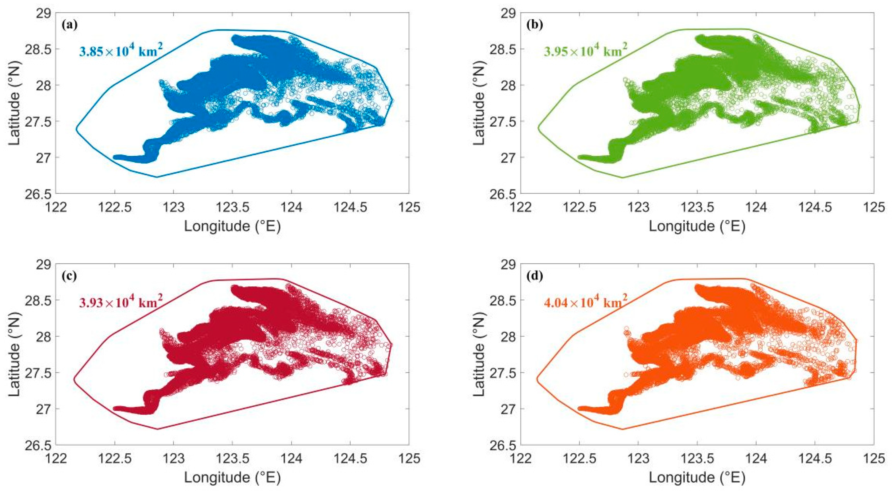
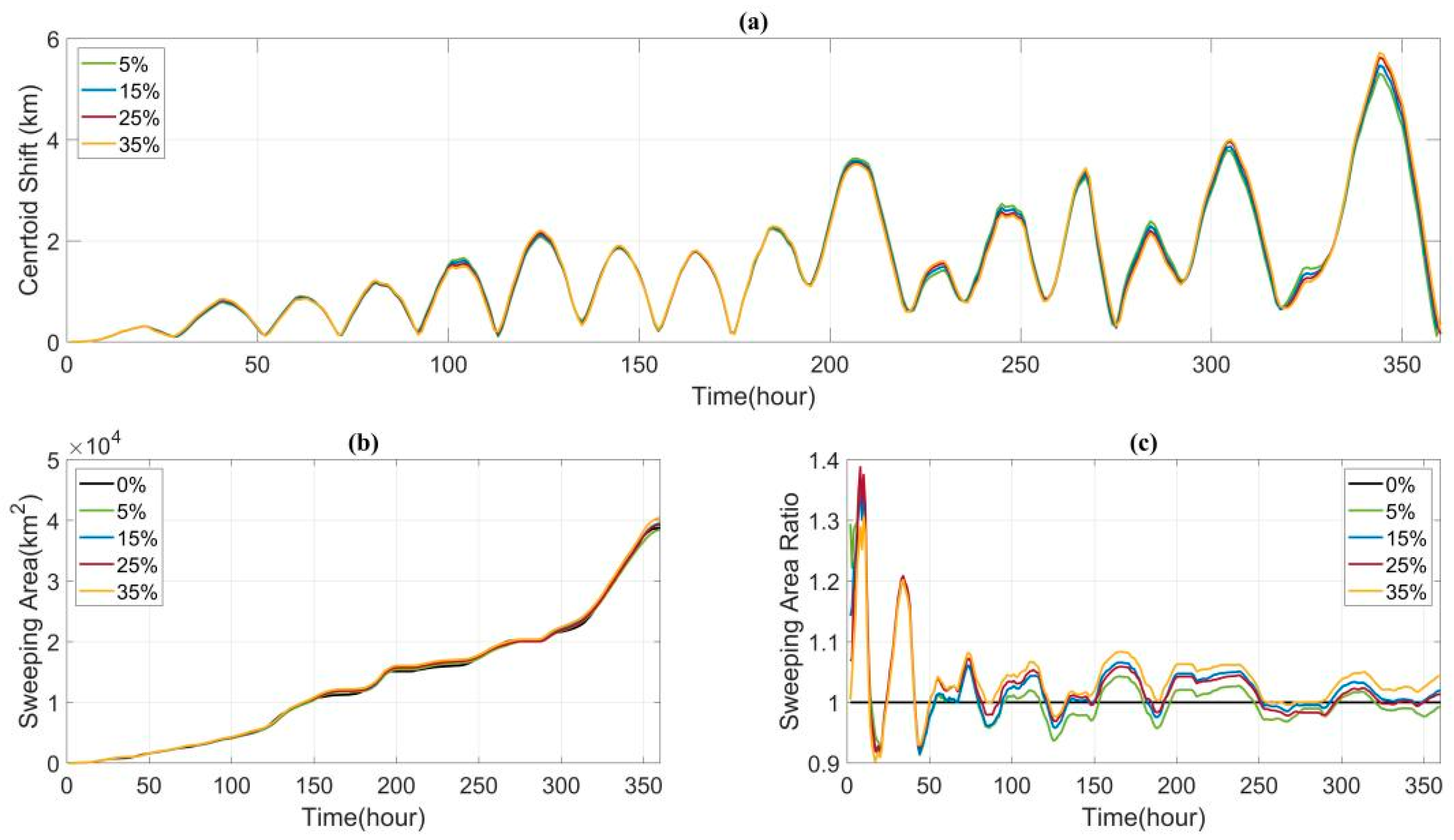
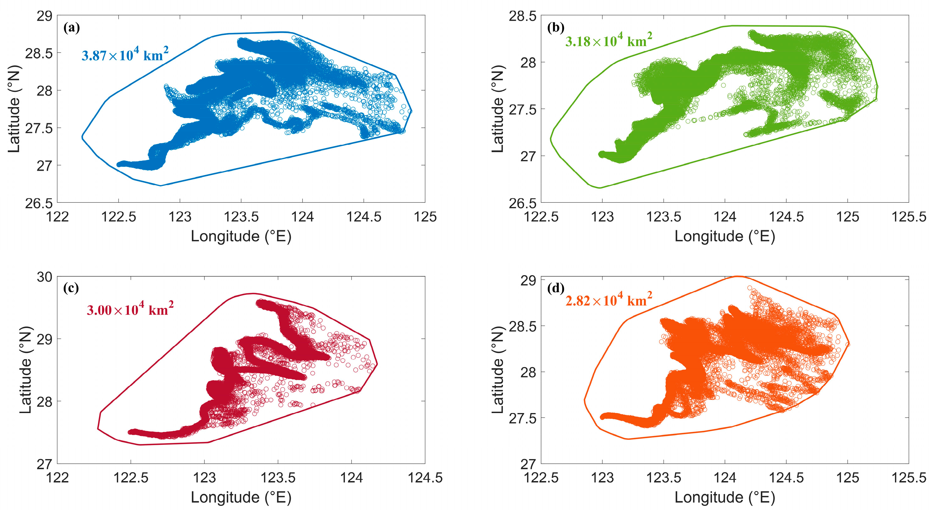
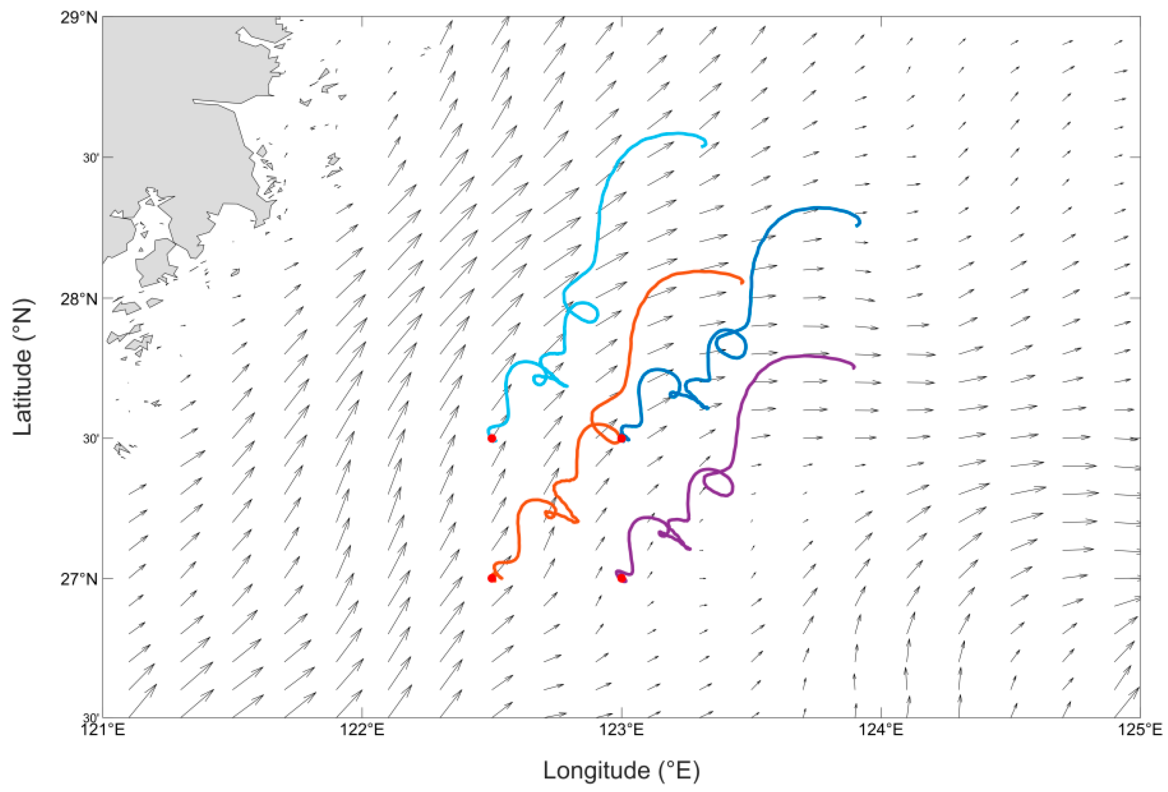
3.2. Impact of Background Flow Field Uncertainty

As shown in Figure 3, after introducing different magnitudes of errors to the background flow field in Experiments 2, 3, 4, and 5, the drift trajectories of the fish-feed pollutants are almost identical to those in Experiment 1 (as shown in Figure 2), with only some minor differences. Their overall movement direction aligns with the direction of the wind and ocean currents. Additionally, in Figure 3a–d, the areas enclosed by solid lines of different colors represent the sweeping areas of the particles in the various experiments. The maximum sweeping areas are 3.85 × 10⁴ km², 3.95 × 10⁴ km², 3.93 × 10⁴ km², and 4.04 × 10⁴ km², respectively, showing an increasing trend as the maximum random error introduced into the background flow field increases.

As shown in Figure 4a, this study calculated the changes over time in the distance between the centroids of all particles in Experiments 2, 3, 4, and 5 and the centroid of the particles in Experiment 1. From Figure 4a, it can be observed that from Experiment 2 to Experiment 5, the impact on the particle-centroid shift distance is roughly the same as the maximum random error introduced into the background flow field increases. During the first 200 h, regardless of the magnitude of the maximum random error introduced, the shift distance between the particle centroids in Experiments 2, 3, 4, and 5 and those in Experiment 1 remains small, generally within 2.29 km. After 200 h, the shift distance between the particle centroids in Experiments 2, 3, 4, and 5 and those in Experiment 1 increases, with the maximum displacement distance reaching approximately 5.72 km. As time progresses, the influence of background flow field uncertainty on centroid displacement increases, and the dispersion of the centroid positions grows.

As shown in Figure 4b, this study calculated the changes in the sweeping area of particles over time in Experiments 1, 2, 3, 4, and 5. From Figure 4b, it can be observed that the sweeping area of particles gradually increases over time, with a trend of increasing growth rate, reaching its maximum value at 360 h. Due to the large value of the sweeping area, the differences in the sweeping areas among different experiments in Figure 4b are not significant. Therefore, this study calculates the ratio of the sweeping areas of particles in Experiments 2, 3, 4, and 5 to that in Experiment 1. The temporal variation of these ratios is shown in Figure 4c.

From Figure 4c, it can be seen that within the first 50 h, the ratio of the sweeping areas of particles in Experiments 2, 3, 4, and 5 to that in Experiment 1 fluctuates greatly. After 50 h, the ratio stabilizes, indicating that the uncertainty of the background flow field has a significant impact on the sweeping area within the first 50 h, and this impact gradually decreases after 50 h. Notably, when the maximum random error added to the background flow field is 35%, the sweeping area is significantly larger than in other cases, suggesting that the sweeping area increases as the maximum random error in the background flow field increases.

Overall, the uncertainty in the background flow field significantly impacts the uncertainty of both the centroid position and the sweeping area in the numerical simulations. When a random error of 35% is introduced into the background flow field, the centroid shift distance reaches its highest value of approximately 5.72 km. Similarly, the sweeping area also reaches its maximum value of 4.04 × 10⁴ km² when the maximum random error of 35% is introduced into the background flow field.

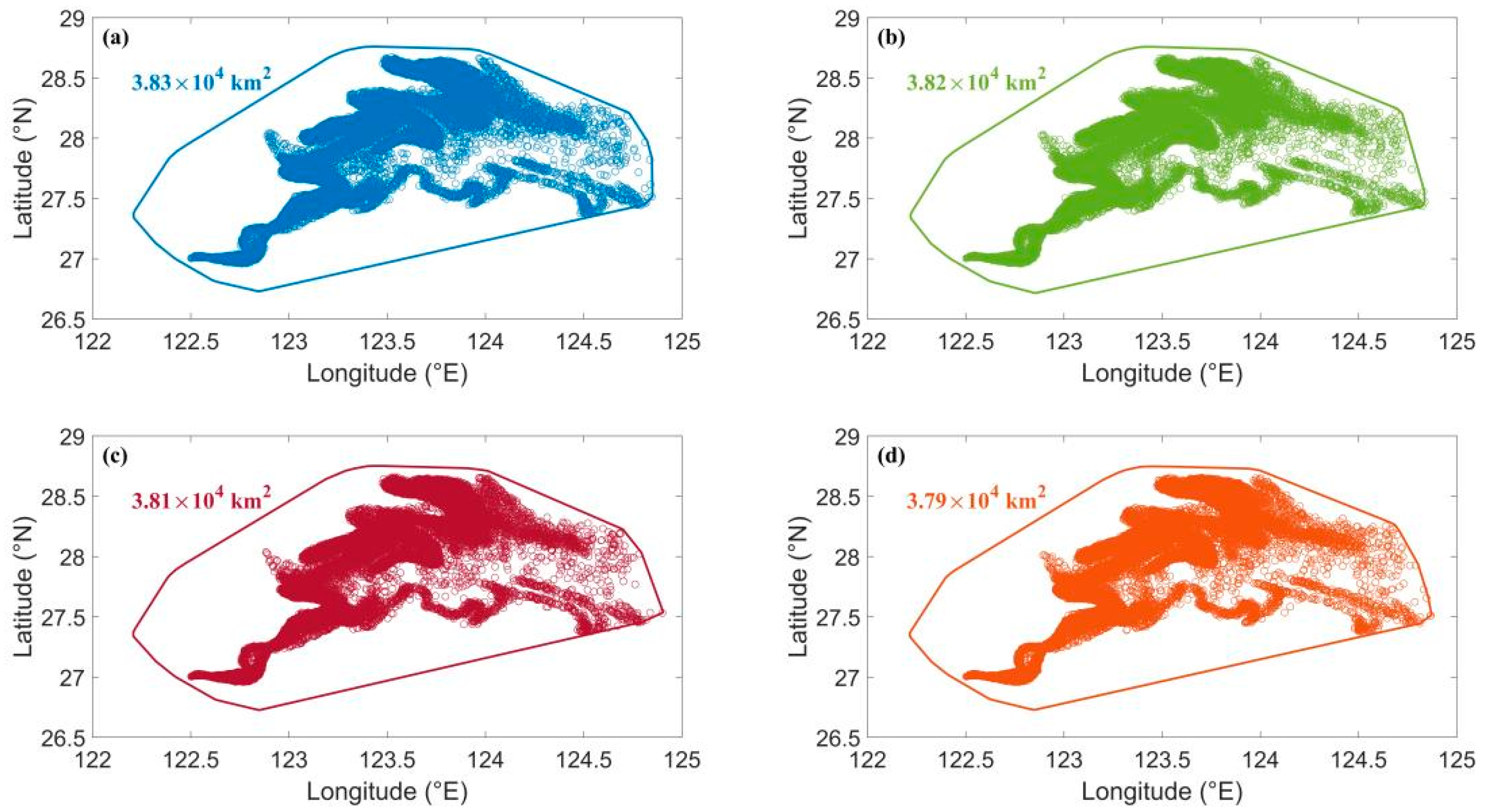
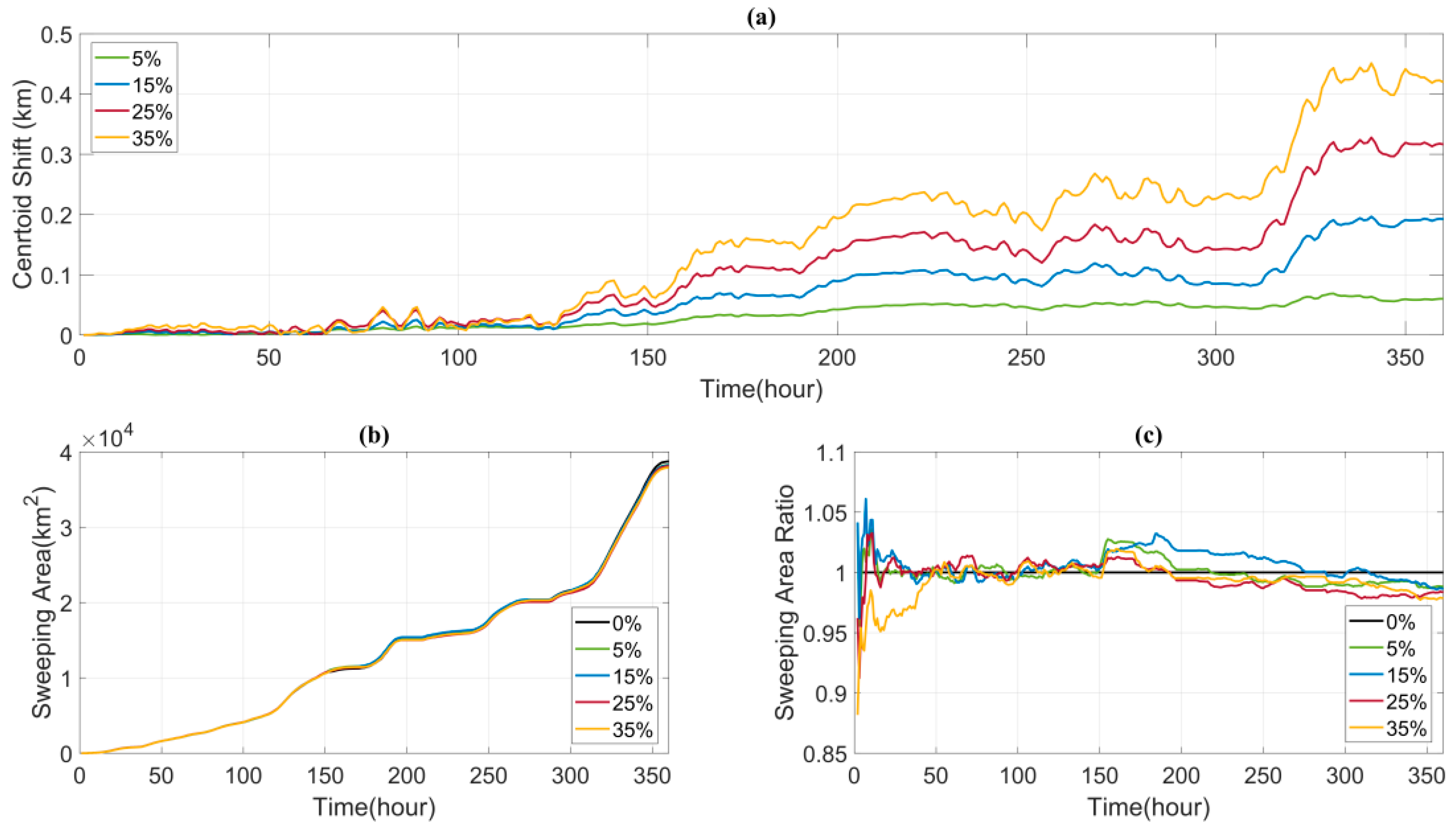
3.3. Impact of Background Wind-Field Uncertainty

As shown in Figure 5, when different levels of random errors are added to the background wind field, the drift trajectories of the feed pollutants remain largely consistent with those observed in Experiment 1, where no errors were added (as shown in Figure 2). In Figure 5a–d, different-colored solid line-enclosed areas represent the sweeping areas of particles from Experiments 6 to 9. The maximum sweeping areas are 3.83 × 10⁴ km², 3.82 × 10⁴ km², 3.81 × 10⁴ km², and 3.79 × 10⁴ km², respectively. These values indicate that as the uncertainty in the background wind field increases, the uncertainty in the sweeping area does not significantly differ from the control experiment.

As shown in Figure 6a, this study calculates the temporal variation in the distance of the centroid shift of all particles in Experiments 6, 7, 8, and 9 relative to the centroid of particles in Experiment 1. From Figure 6a, it can be seen that as the maximum random error added to the background wind field increases from Experiment 6 to Experiment 9, the centroid shift distance of the particles remains within 0.5 km. Before 125 h, the centroid shift distance between particles in Experiments 6, 7, 8, and 9 and those in Experiment 1 is minimal, remaining within 0.04 km. After 125 h, the centroid shift distance between particles in Experiments 6, 7, 8, and 9 and those in Experiment 1 increases with time, and the trend of this increase also grows. Additionally, after 125 h, the greater the random error added to the background wind field at the same time, the greater the centroid shift distance. It is noteworthy that the centroid shift distance, when adding an error only to the background wind field, is much smaller than when adding an error only to the background flow field. This indicates that while the uncertainties in both the background flow field and the background wind field affect the centroid shift distance, the impact of the wind field is much smaller than that of the flow field.

As shown in Figure 6b, this study calculates the variation in the sweeping area of particles over time for Experiments 1, 6, 7, 8, and 9. From Figure 6b, it is evident that the sweeping area of the particles gradually increases over time, with its growth trend becoming more pronounced, reaching a maximum at 360 h. The ratio of the sweeping area of particles in Experiments 6, 7, 8, and 9 to that in Experiment 1 is calculated, and the results over time are shown in Figure 6c. From Figure 6c, it can be observed that within 360 h, the maximum ratios of the sweeping area in Experiments 6, 7, 8, and 9 to that in Experiment 1 are 1.04, 1.06, 1.03, and 1.02, respectively. This further confirms that with the increase in background wind-field uncertainty, the uncertainty in the sweeping area does not differ significantly from the control experiment.

Overall, the uncertainty in the background wind field and background current field affects both the centroid position and the sweeping area of the particles. However, the impact of wind-field uncertainty is significantly less than that of current-field uncertainty. Additionally, in the later stages of the simulation, the output error in the sweeping area does not exceed the input error, indicating that the background field errors are not amplified. The uncertainty caused by the background field errors decreases with the simulation duration. This offers significant insights into the study of the feed-pollutant transport.

3.4. Impact of Different Initial Release Positions

To study the influence of different initial release positions on the simulation results, this research selected different locations (K0, K1, K2, and K3) at the same time to release 100,000 particles to simulate the drift process of fish-feed pollutants, as shown in Figure 7. It can be observed that the drift trajectories of the fish-feed pollutants have similar trends, all drifting northeastward, which is the result of the combined action of ocean currents and winds. At the end of the simulation period of 360 h, the final centroids of experiments 1, 10, 11, and 12 were 150.33 km, 121.06 km, 139.85 km, and 122.12 km away from their respective initial release positions. The selected East China Sea region has a relatively similar marine atmospheric environment, and the differences in latitude and longitude between the initial release positions are within 0.5 degrees. Within the 360 h period, the differences in particle drift distances are within 30 km. Therefore, the different initial release positions have little effect on the drift direction of fish-feed pollutants, but they do have some influence on the drift distance, and they have a significant impact on the final position of the pollutant centroid.

Figure 8 illustrates the schematic diagram of the centroid drift of all particles in experiments 1, 10, 11, and 12 after 15 days. It can be observed from Figure 8 that the centroid drift trajectories of particles show similarity regardless of the different initial release positions. Additionally, within the 360 h period, the centroid trajectories of experiments 1, 10, 11, and 12 hardly intersect.

4. Summary and Conclusions

Based on a Lagrangian particle-tracking algorithm, this study established a model for the drift of fish-feed pollutants in the East China Sea and designed four groups of sensitivity experiments to investigate the impact of model input uncertainties on the drift trajectories, centroid positions, and sweeping areas of fish-feed pollutants. The study found that the uncertainty of the background flow field has a certain influence on the uncertainty of centroid position and sweeping area in numerical simulations. When a random error of 35% is introduced into the background flow field, the centroid shift distance reaches its maximum, and the sweeping area also attains its largest value. The uncertainty of the background wind field influences the centroid position of particles, but the impact is much smaller than the uncertainty of the background flow field. Moreover, when considering only the uncertainty of the background wind field, there is no significant difference in the uncertainty of the sweeping area with the increase in the uncertainty of the background wind field. The difference in initial release positions has little effect on the drift direction and pattern of fish-feed pollutants, but it impacts the drift distance.

When simulating the movement of fish-feed pollutants in seawater, model input uncertainties should be prioritized for consideration, as this can significantly enhance the reliability and predictive capability of the model. In situations with limited resources, accounting for model input uncertainty can assist in optimizing resource allocation and strategy formulation. When designing routes for aquaculture vessels, considering model input uncertainty can facilitate more efficient resource allocation and risk reduction and provide more rational and effective route planning for aquaculture vessels.

References

1. Long, L.; Liu, H.; Cui, M.; Zhang, C.; Liu, C. Offshore Aquaculture in China. Rev. Aquac. 2024, 16, 254–270. [Google Scholar] [CrossRef]
2. Di Trapani, A.M.; Sgroi, F.; Testa, R.; Tudisca, S. Economic Comparison between Offshore and Inshore Aquaculture Production Systems of European Sea Bass in Italy. Aquaculture 2014, 434, 334–339. [Google Scholar] [CrossRef]
3. Davies, I.P.; Carranza, V.; Froehlich, H.E.; Gentry, R.R.; Kareiva, P.; Halpern, B.S. Governance of Marine Aquaculture: Pitfalls, Potential, and Pathways Forward. Mar. Policy 2019, 104, 29–36. [Google Scholar] [CrossRef]
4. Li, L.; Jiang, Z.; Ong, M.C.; Hu, W. Design Optimization of Mooring System: An Application to a Vessel-Shaped Offshore Fish Farm. Eng. Struct. 2019, 197, 109363. [Google Scholar] [CrossRef]
5. Chu, Y.I.; Wang, C.M.; Park, J.C.; Lader, P.F. Review of Cage and Containment Tank Designs for Offshore Fish Farming. Aquaculture 2020, 519, 734928. [Google Scholar] [CrossRef]
6. Aarset, B.; Carson, S.G.; Wiig, H.; Måren, I.E.; Marks, J. Lost in Translation? Multiple Discursive Strategies and the Interpretation of Sustainability in the Norwegian Salmon Farming Industry. Food Ethics 2020, 5, 11. [Google Scholar] [CrossRef]
7. Kim, D.-H.; Lipton, D.; Choi, J.-Y. Analyzing the Economic Performance of the Red Sea Bream Pagrus Major Offshore Aquaculture Production System in Korea. Fish. Sci. 2012, 78, 1337–1342. [Google Scholar] [CrossRef]
8. Schupp, M.F.; Kafas, A.; Buck, B.H.; Krause, G.; Onyango, V.; Stelzenmüller, V.; Davies, I.; Scott, B.E. Fishing within Offshore Wind Farms in the North Sea: Stakeholder Perspectives for Multi-Use from Scotland and Germany. J. Environ. Manag. 2021, 279, 111762. [Google Scholar] [CrossRef] [PubMed]
9. Cao, L.; Wang, W.; Yang, Y.; Yang, C.; Yuan, Z.; Xiong, S.; Diana, J. Environmental Impact of Aquaculture and Countermeasures to Aquaculture Pollution in China. Environ. Sci. Pollut. Res.-Int. 2007, 14, 452–462. [Google Scholar]
10. Xu, Y.F.; Xu, H.; Liu, H.; Kan, Z.X.; Cui, M.C. Research on the Development Way of Deepsea Mariculture in China. Fish Mod. 2021, 48, 9–15. [Google Scholar]
11. Jalón-Rojas, I.; Wang, X.H.; Fredj, E. A 3D Numerical Model to Track Marine Plastic Debris (TrackMPD): Sensitivity of Microplastic Trajectories and Fates to Particle Dynamical Properties and Physical Processes. Mar. Pollut. Bull. 2019, 141, 256–272. [Google Scholar] [CrossRef] [PubMed]
12. Yang, Z.; Chen, Z.; Lee, K.; Owens, E.; Boufadel, M.C.; An, C.; Taylor, E. Decision Support Tools for Oil Spill Response (OSR-DSTs): Approaches, Challenges, and Future Research Perspectives. Mar. Pollut. Bull. 2021, 167, 112313. [Google Scholar] [CrossRef] [PubMed]
13. Wang, N.; Cao, R.; Lv, X.; Shi, H. Research on the Transport of Typical Pollutants in the Yellow Sea with Flow and Wind Fields. J. Mar. Sci. Eng. 2023, 11, 1710. [Google Scholar] [CrossRef]
14. Li, Y.; Chen, H.; Lv, X. Impact of Error in Ocean Dynamical Background, on the Transport of Underwater Spilled Oil. Ocean Model. 2018, 132, 30–45. [Google Scholar] [CrossRef]
15. Jorda, G.; Comerma, E.; Bolaños, R.; Espino, M. Impact of Forcing Errors in the CAMCAT Oil Spill Forecasting System. A Sensitivity Study. J. Mar. Syst. 2007, 65, 134–157. [Google Scholar] [CrossRef]
16. Wang, S.; Iskandarani, M.; Srinivasan, A.; Thacker, W.C.; Winokur, J.; Knio, O.M. Propagation of Uncertainty and Sensitivity Analysis in an Integral Oil-gas Plume Model. J. Geophys. Res. Oceans 2016, 121, 3488–3501. [Google Scholar] [CrossRef]
17. Elliott, A.J.; Jones, B. The Need for Operational Forecasting during Oil Spill Response. Mar. Pollut. Bull. 2000, 40, 110–121. [Google Scholar] [CrossRef]
18. Gonçalves, R.C.; Iskandarani, M.; Srinivasan, A.; Thacker, W.C.; Chassignet, E.; Knio, O.M. A Framework to Quantify Uncertainty in Simulations of Oil Transport in the Ocean. J. Geophys. Res. Oceans 2016, 121, 2058–2077. [Google Scholar] [CrossRef]
19. Browne, M.A.; Galloway, T.S.; Thompson, R.C. Spatial Patterns of Plastic Debris along Estuarine Shorelines. Environ. Sci. Technol. 2010, 44, 3404–3409. [Google Scholar] [CrossRef]
20. Van Sebille, E.; Aliani, S.; Law, K.L.; Maximenko, N.; Alsina, J.M.; Bagaev, A.; Bergmann, M.; Chapron, B.; Chubarenko, I.; Cózar, A.; et al. The Physical Oceanography of the Transport of Floating Marine Debris. Environ. Res. Lett. 2020, 15, 023003. [Google Scholar] [CrossRef]
21. Huang, D.; Chen, H.; Shen, M.; Tao, J.; Chen, S.; Yin, L.; Zhou, W.; Wang, X.; Xiao, R.; Li, R. Recent Advances on the Transport of Microplastics/Nanoplastics in Abiotic and Biotic Compartments. J. Hazard. Mater. 2022, 438, 129515. [Google Scholar] [CrossRef] [PubMed]
22. Uzun, P.; Farazande, S.; Guven, B. Mathematical Modeling of Microplastic Abundance, Distribution, and Transport in Water Environments: A Review. Chemosphere 2022, 288, 132517. [Google Scholar] [CrossRef] [PubMed]
23. Strady, E.; Dang, T.H.; Dao, T.D.; Dinh, H.N.; Do, T.T.D.; Duong, T.N.; Duong, T.T.; Hoang, D.A.; Kieu-Le, T.C.; Le, T.P.Q. Baseline Assessment of Microplastic Concentrations in Marine and Freshwater Environments of a Developing Southeast Asian Country, Viet Nam. Mar. Pollut. Bull. 2021, 162, 111870. [Google Scholar] [CrossRef] [PubMed]
24. Galeao, A.C.; Almeida, R.C.; Malta, S.M.C.; Loula, A.F.D. Finite Element Analysis of Convection Dominated Reaction–Diffusion Problems. Appl. Numer. Math. 2004, 48, 205–222. [Google Scholar] [CrossRef]
25. Saadeh, R. Numerical Solutions of Fractional Convection-Diffusion Equation Using Finite-Difference and Finite-Volume Schemes. J. Math. Comput. Sci. 2021, 11, 7872–7891. [Google Scholar]
26. Aiyer, A.K.; Yang, D.; Chamecki, M.; Meneveau, C. A Population Balance Model for Large Eddy Simulation of Polydisperse Droplet Evolution. J. Fluid Mech. 2019, 878, 700–739. [Google Scholar] [CrossRef]
27. Cao, R.; Chen, H.; Li, H.; Fu, H.; Wang, Y.; Bao, M.; Tuo, W.; Lv, X. A Mesoscale Assessment of Sinking Oil during Dispersant Treatment. Ocean Eng. 2022, 263, 112341. [Google Scholar] [CrossRef]
28. Waldschläger, K.; Schüttrumpf, H. Effects of Particle Properties on the Settling and Rise Velocities of Microplastics in Freshwater under Laboratory Conditions. Environ. Sci. Technol. 2019, 53, 1958–1966. [Google Scholar] [CrossRef] [PubMed]
29. Stolzenbach, K.D.; Madsen, O.S.; Adams, E.E.; Pollack, A.M.; Cooper, C. A Review and Evaluation of Basic Techniques for Predicting the Behavior of Surface Oil Slicks; Massachusetts Institute of Technology Sea Grant Program: Cambridge, MA, USA, 1977. [Google Scholar]
30. Samuels, W.B.; Huang, N.E.; Amstutz, D.E. An Oilspill Trajectory Analysis Model with a Variable Wind Deflection Angle. Ocean Eng. 1982, 9, 347–360. [Google Scholar] [CrossRef]
31. Wang, J.; Shen, Y. Modeling Oil Spills Transportation in Seas Based on Unstructured Grid, Finite-Volume, Wave-Ocean Model. Ocean Model. 2010, 35, 332–344. [Google Scholar] [CrossRef]
32. Pan, Q.; Yu, H.; Daling, P.S.; Zhang, Y.; Reed, M.; Wang, Z.; Li, Y.; Wang, X.; Wu, L.; Zhang, Z. Fate and Behavior of Sanchi Oil Spill Transported by the Kuroshio during January–February 2018. Mar. Pollut. Bull. 2020, 152, 110917. [Google Scholar] [CrossRef] [PubMed]
33. Boufadel, M.; Liu, R.; Zhao, L.; Lu, Y.; Özgökmen, T.; Nedwed, T.; Lee, K. Transport of Oil Droplets in the Upper Ocean: Impact of the Eddy Diffusivity. J. Geophys. Res. Oceans 2020, 125, e2019JC015727. [Google Scholar] [CrossRef]
34. Bandara, U.C.; Yapa, P.D. Bubble Sizes, Breakup, and Coalescence in Deepwater Gas/Oil Plumes. J. Hydraul. Eng. 2011, 137, 729–738. [Google Scholar] [CrossRef]
35. Rong, Z.; Li, M. Tidal Effects on the Bulge Region of Changjiang River Plume. Estuar. Coast. Shelf Sci. 2012, 97, 149–160. [Google Scholar] [CrossRef]
36. Egbert, G.D.; Bennett, A.F.; Foreman, M.G.G. TOPEX/POSEIDON Tides Estimated Using a Global Inverse Model. J. Geophys. Res. Oceans 1994, 99, 24821–24852. [Google Scholar] [CrossRef]
37. Cao, R.; Chen, H.; Rong, Z.; Lv, X. Impact of Ocean Waves on Transport of Underwater Spilled Oil in the Bohai Sea. Mar. Pollut. Bull. 2021, 171, 112702. [Google Scholar] [CrossRef] [PubMed]
38. Haidvogel, D.B.; Blanton, J.; Kindle, J.C.; Lynch, D.R. Coastal Ocean Modeling: Processes and Real-Time Systems. Oceanography 2000, 13, 35–46. [Google Scholar] [CrossRef]
39. Shchepetkin, A.F.; McWilliams, J.C. The Regional Oceanic Modeling System (ROMS): A Split-Explicit, Free-Surface, Topography-Following-Coordinate Oceanic Model. Ocean. Model. 2005, 9, 347–404. [Google Scholar] [CrossRef]
40. Egbert, G.D.; Erofeeva, S.Y. Efficient Inverse Modeling of Barotropic Ocean Tides. J. Atmos. Ocean Technol. 2002, 19, 183–204. [Google Scholar] [CrossRef]
41. Chapman, D.C. Numerical Treatment of Cross-Shelf Open Boundaries in a Barotropic Coastal Ocean Model. J. Phys. Oceanogr. 1985, 15, 1060–1075. [Google Scholar] [CrossRef]
42. Flather, R.A. A Tidal Model of the Northwest European Continental Shelf. Mem. Soc. Roy. Sci. Liege 1976, 10, 141–164. [Google Scholar]
43. Orlanski, I. A Simple Boundary Condition for Unbounded Hyperbolic Flows. J. Comput. Phys. 1976, 21, 251–269. [Google Scholar] [CrossRef]
44. Khater, E.-S.G.; Bahnasawy, A.H.; Ali, S.A. Physical and Mechanical Properties of Fish Feed Pellets. J. Food Process Technol. 2014, 5, 1. [Google Scholar]
45. Wang, J.Z.; Wang, Y.; Jiang, P. The Study and Application of a Novel Hybrid Forecasting Model—A Case Study of Wind Speed Forecasting in China. Appl. Energy 2015, 143, 472–488. [Google Scholar] [CrossRef]
46. Wang, D.; Luo, Z.; Mu, L. Numerical Study on the Influence of Model Uncertainties on the Transport of Underwater Spilled Oil. Int. J. Environ. Res. Public Health 2022, 19, 9274. [Google Scholar] [CrossRef]
47. Chen, Y.; Huang, W.; Shan, X.; Chen, J.; Weng, H.; Yang, T.; Wang, H. Growth Characteristics of Cage-Cultured Large Yellow Croaker Larimichthys Crocea. Aquac. Rep. 2020, 16, 100242. [Google Scholar] [CrossRef]
Figure 1. Map of the East China Sea study area. K0 (red pentagon), K1 (blue square), K2 (green circle), and K3 (yellow triangle) represent the initial release positions of particles for the simulation.
Jmse 12 01196 g001
Figure 2. Particle distribution after 15 days of model simulation with the initial release position at K0. The area enclosed by a red solid line represents the sweeping area of the particles, with its value indicated by the same color. The red hollow circles represent the positions of the particles after 15 days of simulation.
Jmse 12 01196 g002
Figure 3. Particle distribution after 15 days of model simulation in (a) Experiment 2, (b) Experiment 3, (c) Experiment 4, and (d) Experiment 5. The areas enclosed by solid lines of different colors correspond to the sweeping areas of the particles in each experiment, with their values indicated by the same color.
Jmse 12 01196 g003
Figure 4. (a) The temporal variation of the distance between the centroids of all particles in Experiments 2, 3, 4, and 5 and the centroid of particles in Experiment 1. (b) The temporal variation of the sweeping areas in Experiments 1, 2, 3, 4, and 5. (c) The ratio of the sweeping areas of particles in Experiments 2, 3, 4, and 5 to that in Experiment 1 over time.
Jmse 12 01196 g004
Figure 5. Particle distribution after 15 days of model simulation in (a) Experiment 6, (b) Experiment 7, (c) Experiment 8, and (d) Experiment 9. The areas enclosed by solid lines of different colors correspond to the sweeping areas of the particles in each experiment, with their values indicated by the same color.
Jmse 12 01196 g005
Figure 6. (a) The temporal variation of the distance between the centroids of all particles in Experiments 6, 7, 8, and 9 and the centroid of particles in Experiment 1. (b) The temporal variation of the sweeping areas of particles in Experiments 1, 6, 7, 8, and 9. (c) The ratio of the sweeping area of particles in Experiments 6, 7, 8, and 9 to that in Experiment 1 over time.
Jmse 12 01196 g006
Figure 7. Particle distribution after 15 days of model simulation in (a) Experiment 1, (b) Experiment 10, (c) Experiment 11, and (d) Experiment 12. The areas enclosed by solid lines of different colors correspond to the sweeping areas of the particles in each experiment, with their values indicated by the same color.
Jmse 12 01196 g007
Figure 8. Trajectories of particle centroids for 15 days starting from April 16th at locations K1, K2, K3, and K4. Arrows represent the average surface flow field of seawater. Different colors represent different initial release positions.
Jmse 12 01196 g008