Laboratory Study on Wave Attenuation by Elastic Mangrove Model with Canopy

Abstract

This study evaluates the effectiveness of artificial Kandelia obovata forests in wave attenuation through physical model experiments conducted in a wave flume. The experiments meticulously replicated real-world hydrodynamic conditions and mangrove movement responses using the principles of gravitational and motion similarity, with a scaled 1:10 model of Kandelia obovata. Our approach included comparative experiments against a 1:100 gradient concrete slope to isolate the effects of seabed friction and flume wall reflections. The wave height was measured using strategically placed wave gauges. The findings indicated that the artificial Kandelia obovata forests significantly attenuated waves, with a decrease in the total attenuation capacity as the water depth increased from 2.75 m to 3.28 m under both regular and irregular waves. The elastic mangrove model with a canopy effect led to a 15% increase in wave attenuation over cylindrical models. Predictive models using multivariate nonlinear regression and back propagation neural networks showed that the latter provided a superior accuracy in estimating wave transmission coefficients

1. Introduction

Mangrove forests, such as Kandelia obovate, are crucial for coastal protection due to their wave attenuation capabilities, reducing the impacts of erosion and storm surges [1,2,3,4,5,6,7]. Considering this, research into wave attenuation within mangroves has not only underscored their importance, but also led to their strategic integration as part of hybrid coastal protection strategies, often combined with sea dikes and beach nourishment projects [8,9]. In the southern Zhejiang region, Kandelia obovata stands out as the sole mangrove species capable of being transplanted, thereby occupying a crucial position in bolstering the coastal defenses in this locale, as documented by Ren, et al. [10]. Investigations into the wave attenuation properties of mangroves date back relatively early due to the recognized capacity of mangrove systems to effectively dampen the waves along coastal stretches. The study of how mangroves attenuate wave energy has, thus, been an ongoing area of inquiry, given their natural effectiveness in mitigating coastal wave impacts.

Field observations constitute the bedrock of research data and play a pivotal role in enhancing our comprehension of mangrove wave attenuation theories. In a noteworthy study, Quartel, Kroon, Augustinus, Van Santen, and Tri [6] ventured into the field to investigate the wave-damping effect of mangroves within Vietnam’s Red River Delta, treating these ecosystems as supplementary sources of frictional resistance. Their findings revealed that the presence of mangrove forests amplified the sandy seabed’s frictional resistance by a factor ranging from 5 to 7.5 times its original value, which aligns closely with the results reported by Mullarney, et al. [11]. Separately, Mazda, et al. [12] discovered through field-based research that the intricate network of branches and leaves inherent to mangrove vegetation significantly contributes to the dissipation of ocean waves. They further provided an empirical formula linking plant characteristics, water depth, and prevailing wave conditions. Horstman, et al. [13] used field data and spectral models to analyze the wave attenuation characteristics of mangroves on the west coast of Thailand. Their findings indicated that a mangrove belt with a width spanning 246 m reduced the effective wave height ($H_s$) by 42% to 47%. Additionally, the study found that the greater the incident wave height and the lower the relative water depth, the better the wave attenuation effect of the mangrove belt. Vo-Luong and Massel [14], in another investigation, monitored changes in $H_s$, wave frequency spectrum density, and flow velocity when random waves transversed through a non-uniform mangrove belt. They utilized mild-slope equations to simulate the wave behavior within the mangrove region. The outcomes of this research highlighted that both wave-breaking phenomena and the complex interactions between waves and the branches of mangrove trees were instrumental in dissipating wave energy. When the density of mangroves was lower, wave energy dissipation predominantly occurred due to wave-breaking events; conversely, in denser mangrove settings, the structural elements of the mangrove vegetation played a more pronounced role in mitigating wave energy. Brinkman, et al. [15], through field observations, revealed that when waves pass through mangroves, there is no obvious change in the wave frequency spectrum of different periods, indicating that waves of different periods damped at approximately the same rate.

There are some differences between field observations and experiments. Experimental research conducted by Wu and Cox [16] revealed that plants exhibit better wave attenuation effects on high-frequency waves under shallow water conditions. Additionally, when the relative water depth ($d/h$, the ratio of the water depth to the height of mangrove) increased, the degree of wave height attenuation also increased, suggesting that, when the non-linearity of waves strengthens, the wave attenuation effect of plants is better. Augustin, et al. [17] performed a physical experiment to study wave damping under nearly submerged and unsubmerged rigid vegetation. The results indicated a superior wave attenuation by rigid plants in non-submerged conditions compared to when they were nearly submerged. The drag coefficient of unsubmerged plants exhibited a stronger link with the Reynolds number ($Re$), likely because the main wave energy is concentrated close to the water surface.

The experiments mentioned earlier were premised on the simplifying assumption that mangrove trees behave as rigid cylinders, which does not accurately capture the complex movement responses of mangroves to hydrodynamic forces and their unique vertical structure. Unlike fully flexible plant stems and canopies, mangrove stems exhibit a certain degree of elasticity. As such, treating them as completely rigid introduces a departure from their actual physical dynamics. According to Bouma, et al. [18], under comparable wave conditions, the drag force exerted by rigid mangrove stems is around three times greater than that generated by more flexible plants. In a similar vein, van Veelen, et al.’s [19] experiment showed that wave attenuation by flexible pile groups is about 70% smaller than rigid pile groups.

Several research studies have focused on the vertical morphology of mangrove forests [20,21,22,23,24,25]. Generally, mangrove vertical morphology can be divided into three distinct layers, i.e., canopy, stem, and roots. The vertically varying density effects on wave attenuation are much significant under deep water waves [24]. As for roots, a few researchers [22,25,26,27,28,29] with a scale ratio ranging from 1:1 to 1:12 have proved that planted mangrove with roots can be effective in wave attenuation and protecting coastal areas. Nonetheless, despite exhaustive examinations of the hydrodynamic influences on the consistently submerged prop roots and lower trunks of mature mangrove trees in prior studies, scant attention has been directed towards the unique case of the canopy in juvenile saplings and stunted mangroves, which may also find themselves submerged under conditions of heightened water levels. Both field observations [12] and laboratory experiments [20,23] have indicated the strong potential for wave attenuation by mangrove with dense canopies. Those researchers proved that the canopy and roots cannot be ignored in wave attenuation by mangroves. Consequently, while qualitative appreciations are abound, a quantitative understanding of the specific contribution made by an elastic mangrove model to wave attenuation, particularly when considering the inclusion of canopies, remains a gap in our knowledge.

This study uses laboratory experiments to explore the hydrodynamic behavior of a Kandelia obovata model with elasticity and vertically varying structures under different water depths in response to wave action. The wave conditions and physical representations of the plants are carefully designed based on field surveys, ensuring that the experimental setup reflects actual environmental conditions. Recognizing that linear wave theory may not accurately depict the dynamics of waves in complex environments such as finite-depth waves with sloping bottoms, this research utilizes finite-depth wave mechanics as a basis for its analysis. To enhance the accuracy of predicting the wave attenuation within artificial Kandelia obovata forests, sophisticated statistical tools like multivariate nonlinear regression (MNLR) and back propagation (BP) neural networks (for further specifics, refer to Malvin, et al. [30] and Yin, et al. [31]) are employed to develop a predictive model for the wave attenuation coefficient.

2. Theoretical Background

Considering the methods for calculating wave attenuation, many works have been conducted. Of which, Equation (1) [32] has received extensive attention and ongoing research.

$$K_V\left(x\right)={\displaystyle \frac{H_s\left(x\right)}{H_{s,i}}}={\displaystyle \frac{1}{1+\beta x}}$$

(1)

where $K_V\left(x\right)$ is the wave transmission coefficient as a function of distance through the plant bed; $H_s\left(x\right)$ is the significant wave height at a distance $x$ through the plant bed; $H_{s,i}$ is the significant wave height at the leading edge of the vegetation; and $\beta$ is a damping factor. For irregular waves [33],

$$\beta ={\displaystyle \frac{1}{3\sqrt{\pi }}}{C}_{D}DN{H}_{rms}k{\displaystyle \frac{{\sinh }^{3}ks+3\sinh ks}{\left(\sinh 2kd+2kd\right)\sinh kd}}$$

(2)

where $C_D$ is a bulk drag coefficient, $N$ is the vegetation density (stems/m²), $D$ is the diameter of the stem, $s$ is the submerged height of the vegetation, $H_{rms}$ is the root-mean-square wave height estimated as $H_s$ = 1.416 $H_{rms}$ using the Rayleigh distribution, $k$ is the wave number of the peak in the spectrum, and $d$ is the still water depth.

It must be noted that Equations (1) and (2) are based on assumptions that vegetation is simplified into a rigid cylinder group and the linear wave theory is suitable. The aim of the present work is to obtain a prediction method applicable for assessing wave attenuation by Kandelia obovavta on a slope through physical model experiments.

As for $C_D$, several studies [21,23,26,27,34] have taken vertical morphology into consideration. These existing empirical formulas for the bulk drag coefficient of mangroves under waves are summarized in

Table 1. Existing empirical formulas of C_D for vertically varying mangrove under waves.

No.	Source	Scale Ratio	Vegetation	Formula	Scope
1	Maza, Adler, Ramos, Garcia, and Nepf [34]	1:12	Model with stem and root	$C_D=9.49\times {{Re}_d}^{1.41}$	500 < ${Re}_d$ < 1700
2	He, Chen, and Jiang [23]	1:10	Model with stem, root, and canopy	$C_D=18.025\times {\mathrm{e}}^{-0.043{KC}_d}$	10 < ${KC}_d$ < 37
3	Wang, Yin, and Liu [21]	1:10	Model with stem and root	$C_D=0.42+{\left({\displaystyle \frac{0.77}{{KC}_{rv}}}\right)}^{0.41}$	0.01 < ${KC}_{rv}$ < 0.28
4	Chang, Mori, Tsuruta, Suzuki, and Yanagisawa [27]	1:7	Model with stem and root	$C_D=1.15+{\left({\displaystyle \frac{14.7}{{KC}_{rv}}}\right)}^{1.065}$ $C_D=1.15+{\left({\displaystyle \frac{1015}{{Re}_d}}\right)}^{1.044}$	2.5 < ${Re}_d$ < 20 180 < ${Re}_d$ < 1300
5	Bryant, et al. [35]	1:2.1	Model with stem and root	$C_D=0.86+{\left({\displaystyle \frac{1.24}{{KC}_d}}\right)}^{0.78}$	0 < ${Re}_d$ < 12
6	Kelty, Tomiczek, Cox, Lomonaco, and Mitchell [26]	1:1	Model with stem and root	$C_D=0.60+{\left({\displaystyle \frac{300000}{{Re}_d}}\right)}^{1.0}$	0 < ${Re}_d$ < 12
7	Zhang, Chen, Lei, Zhou, Yao, and Stive [20]	1:10	Model with stem, root, and canopy	$C_D=0.60+{\left({\displaystyle \frac{101.99}{{KC}_d}}\right)}^{1.22}$ $C_D=0.60+{\left({\displaystyle \frac{420000}{{Re}_{rv}}}\right)}^{1.41}$ $C_D=0.60+{\left({\displaystyle \frac{80}{Ur}}\right)}^{0.75}$	500 < ${Re}_d$ < 1700 34,900 < ${Re}_{rv}$ < 40,700 0.73 < $Ur$ < 21.33

.

Where ${Re}_d$ is the Reynolds number’s base on the diameter of the stem and is given by ${Re}_d=U_{max}{D}_{\mathrm{s}\mathrm{t}\mathrm{e}\mathrm{m}}/\nu$; $U_{max}$ is the maximum flow velocity; $D_{\mathrm{s}\mathrm{t}\mathrm{e}\mathrm{m}}$ is the diameter of the stem; $\nu$ is the kinematic viscosity; ${KC}_d$ is the Keulegan–Carpenter number’s base on the diameter of the stem and is given by ${KC}_d=U_{max}T/D_{\mathrm{s}\mathrm{t}\mathrm{e}\mathrm{m}}$; $U_{max}$ is the maximum horizontal orbital velocity; $T$ is the wave period; ${KC}_{rv}$ is the Keulegan–Carpenter number’s base on the hydraulic radius ($r_v$) [36] and is given by ${KC}_d=U_{p}T/r_v$; $U_p$ represents the mean pore velocity that denotes the spatially averaged flow velocity in the spaces among vegetation stems and is given by $U_p=U_{max}/(1-\varphi )$; and $(1-\varphi )$ indicates that the volume fraction of the vegetation is excluded because the wave force only exerts on the wave volume [37]. ${Re}_{rv}$ is the Reynolds number’s base on the hydraulic radius and is given by ${Re}_{rv}=U_{max}{D}_{\mathrm{s}\mathrm{t}\mathrm{e}\mathrm{m}}/r_v$.

Although experiments have taken mangrove with vertical variation into consideration, Equation (3) [23] is limited in cylinder group models due to the complexity of the mechanism in wave attenuation by mangroves. According to their experiments, the mean $C_D$ for a model with a canopy is about 7.

$$C_D={\displaystyle \frac{23.326e^{-0.601Wr}}{{Wr}^{0.24}}}$$

(3)

where $Wr$ is the modified Ursell number and $Wr=Ur/{\alpha }^{-2.338}$ ($0.25<Wr<10$). Equation (4) is deduced based on a rigid cylinder model with a canopy [20].

$$C_D=0.60+{\left({\displaystyle \frac{80}{Ur}}\right)}^{0.75}$$

(4)

The factors influencing the wave attenuation capabilities of mangroves can be grouped into two overarching categories [17]. The first category encompasses hydrodynamic parameters, which include the slope gradient ($i$), the incident wave height ($H_{s,i}$), the incident wave mean period ($T_{m,i}$), and the water depth ($d$). The second category pertains to the inherent characteristics of the Kandelia obovata forest itself, such as its width ($B$), submerged height ($s$), and spatial spacing ($m,n$ represent the horizontal distances in the onshore and alongshore directions, respectively), as well as the spatial features of the canopy, stem, and root.

In the present study, certain simplifications have been made to better understand and isolate the effects of these influential factors. These include focusing on specific aspects of the 4-year-old mangroves’ geometry and positioning relative to the prevailing wave conditions, thereby providing a clearer picture of which factors contribute most significantly to the overall wave-dampening effect.

• Field Survey and Model Creation. Detailed measurements of the plant’s spatial features were obtained through field surveys and utilized for creating corresponding Kandelia obovata models. Detailed parameters of the plant space can be referred to in the subsequent Section 3.2.
• Control Experimental Conditions. The slope was kept constant in the present experiments, allowing to isolate and focus on other variables without the confounding effects of terrain slope variability. This constancy ensures uniformity in the influences of sidewall effects, bottom friction, and slope on the hydrodynamic behavior of waves.

Consequently, the expression for $K_V\left(x\right)$ can be described by the following set of independent variables:

$$K_V\left(x\right)=\phi \left(T_m;H_i;d;B;H_{ko};m;n\right)$$

(5)

where φ stands for function.

In order to isolate and quantify the exclusive influence of Kandelia obovata on wave attenuation, the background or control test attenuation is first deducted from the overall attenuation observed. This process allows for a clear understanding of how much wave energy is being dissipated solely due to the presence of the artificial mangrove forest. Following the methodology outlined by Augustin, Irish, and Lynett [17], the vegetation transmission coefficient ($K_V$) is given as:

$$K_V=K_t+\left(1-K_b\right)$$

(6)

where $K_t$ is the total wave attenuation and $K_b$ is the wave attenuation caused by shallow water effects, bottom frictional effects, and the boundary effect by the walls of the wave flume. Data collected in the control group and experimental group were used to calculate $K_b$ and $K_t$, respectively. Similar expressions can be seen in Maza, Lara, and Losada [28] and Hu, et al. [38].

3. Experimental Setup and Procedures

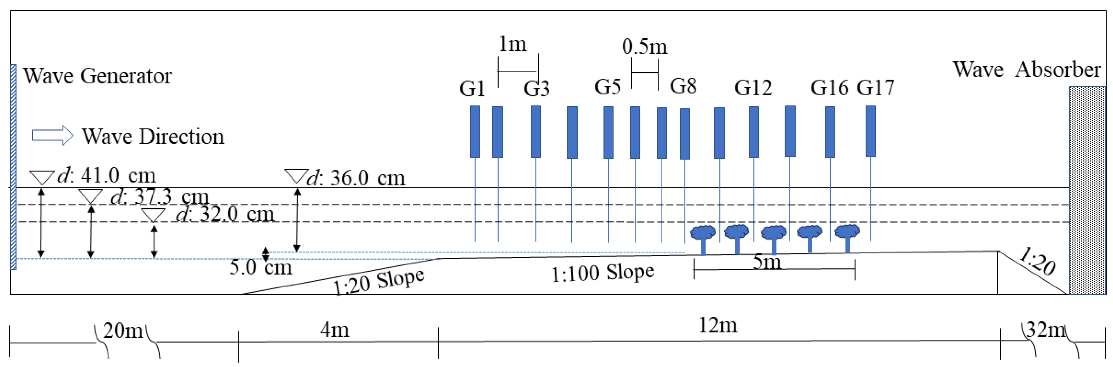
3.1. Experimental Facilities and Instrumentation

The present experimental setup was conducted in a rectangular wave flume, measuring 68 m in length, 1 m in width, and 1.5 m in depth, which is situated at the Tianjin Research Institute for Water Transport Engineering, Ministry of Transportation, Tianjin, China. This specialized facility is equipped with advanced features to ensure accurate and reliable testing. At one end of the flume, there are piston-type wave generators that incorporate an active wave absorption system. These devices generate waves of varying characteristics according to the research requirements and are designed to simulate realistic wave conditions in coastal environments. At the opposite end of the flume, a slope was constructed using gravel blocks and multi-pore media materials. This configuration serves as an efficient wave absorber, reducing the impact of wave reflections, thus ensuring that the experimental outcomes are not distorted by unwanted reflected waves. The reflection coefficients calculated using Goda’s two-point method for the experiments using regular waves (B5, B6, B16B17, B26, B27, B28, B29, B30, B31, and B32) were 0.06, 0.07, 0.08, 0.09, 0.13, 0.09, 0.12, 0.08, 0.08, 0.07, 0.09, and 0.08 (using two measuring points, G1 and G2). To meticulously track the changes in the wave properties along the flume, a total of 17 wave gauges were strategically placed throughout the test area. These instruments measured the wave height, providing detailed data on how it changed over the course of the experiments. A visual representation of this setup, including the placement of the wave gauges, is depicted in Figure 1. Slopes with a 1:20 gradient were used on both sides of the flume. The 1:20 slope was implemented near the wave generator, because the waves in the experiment had a high steepness, making it challenging to generate such waves directly from the wave maker without causing them to break. Instead, generating waves with lower heights and then passing them through the 1:20 gentle slope efficiently increased their effective height to the desired target levels. For the convenience of the operators, a sloped section was also installed at the wave absorber.

As illustrated in Figure 1, wave gauges G1–G7 are strategically positioned to monitor the longitudinal variations in the waves along the mild slope. These gauges served as reference points and were used for validation purposes in both the experimental and control groups, ensuring that all sections experienced the same wave conditions. The sensors G1 and G2 were positioned with an interval of 0.5 m, while the spacings between G2, G3, G4, and G5 were 1 m. Furthermore, the distances separating G5, G6, and G7 were also 0.5 m. Wave gauges G8–G15, with a consistent spacing of 0.5 m between them, were specifically designed to track the longitudinal changes in the wave characteristics when passing through the mangrove models. G8 was located at the very edge of the artificial mangrove forest model, while G16 and G17 were set 1 m away from the previous numbered sensor, allowing for more detailed measurements at varying distances from the mangrove vegetation. In this study, we conducted two sets of experiments on the same terrain to assess the impact of mangrove forests on wave attenuation. The terrain consisted of a 1:100 scale smooth concrete slope. Initially, as a control setup, experiments were performed without any vegetation to collect baseline data. Subsequently, the same slope was equipped with an artificial Kandelia obovata forest model for the experimental setup, allowing the researchers to analyze the effects of the mangroves on wave attenuation under controlled laboratory conditions.

3.2. Experimental Conditions and Experimental Similarity

Previous studies have demonstrated that the hydrodynamic performance of Kandelia obovata forests under wave action is significantly influenced by both the prevailing wave conditions and the characteristics of the vegetation itself. Hence, it is crucial to select appropriate wave and vegetation scenarios for experimental investigations. To this end, a field survey was carried out in Yueqing City, Zhejiang Province, to gather data on the local wave conditions and vegetative features. As for the field survey of the local wave conditions from Feb to Apr 2018, BRB virtuoso3 wave rider buoys were chosen. The collected data were utilized to validate the SWAN model [39], which subsequently estimated the wave heights and periods for various return periods in this area. Validation confirmed that the $H_s$ for 50-year and 2-year return periods was, respectively, 1.8 m and 0.8 m.

Considering the experimental constraints and research objective, the current experiments employed a 1:10 scale physical model. This scaled-down model adhered to the principle of gravitational similarity to emulate real-world hydrodynamic forces and the principle of motion similarity to simulate the actual movement responses of Kandelia obovata when subjected to waves. A detailed comparison between the hydrodynamic conditions in the prototype environment and those replicated within the models is presented in

Table 2. The comparison of hydrodynamic conditions in prototype and model.

Case	Prototype			Model (G1)			Model (G8)			Wave Type	With Mangrove Model or Not
	$\mathit{d}$(m)	${\mathit{T}}_{\mathit{m}}$(s)	${\mathit{H}}_{\mathit{s}}$(m)	$\mathit{d}$(m)	${\mathit{T}}_{\mathit{m}}$(s)	${\mathit{H}}_{\mathit{s}}$(m)	$\mathit{d}$(m)	${\mathit{T}}_{\mathit{m}}$(s)	${\mathit{H}}_{\mathit{s}}$(m)
A1	4.1	6.0	1.8	0.41	1.90	0.18	0.36	1.90	0.16	Irregular	No Model
A2	4.1	5.0	1.5	0.41	1.58	0.15	0.36	1.58	0.14	Irregular	No Model
A3	4.1	4.0	1.2	0.41	1.26	0.12	0.36	1.26	0.10	Irregular	No Model
A4	4.1	3.0	0.8	0.41	0.95	0.08	0.36	0.95	0.08	Irregular	No Model
A5	3.73	6.0	1.8	0.373	1.90	0.18	0.323	1.90	0.14	Irregular	No Model
A6	3.73	5.0	1.5	0.373	1.58	0.15	0.323	1.58	0.14	Irregular	No Model
A7	3.73	6.0	1.5	0.373	1.90	0.15	0.323	1.90	0.14	Irregular	No Model
A8	3.73	7.0	1.2	0.373	2.21	0.12	0.323	2.21	0.13	Irregular	No Model
A9	3.73	6.0	1.2	0.373	1.90	0.12	0.323	1.90	0.11	Irregular	No Model
A10	3.73	5.0	1.2	0.373	1.58	0.12	0.323	1.58	0.12	Irregular	No Model
A11	3.73	4.0	1.2	0.373	1.26	0.12	0.323	1.26	0.11	Irregular	No Model
A12	3.73	6.0	0.8	0.373	1.90	0.08	0.323	1.90	0.09	Irregular	No Model
A13	3.73	3.0	0.8	0.373	0.95	0.08	0.323	0.95	0.05	Irregular	No Model
A14	3.2	5.0	1.5	0.32	1.58	0.15	0.27	1.58	0.12	Irregular	No Model
A15	3.2	6.0	1.5	0.32	1.90	0.15	0.27	1.90	0.12	Irregular	No Model
A16	3.2	7.0	1.2	0.32	2.21	0.12	0.27	2.21	0.12	Irregular	No Model
A17	3.2	6.0	1.2	0.32	1.90	0.12	0.27	1.90	0.12	Irregular	No Model
A18	3.2	5.0	1.2	0.32	1.58	0.12	0.27	1.58	0.12	Irregular	No Model
A19	3.2	4.0	1.2	0.32	1.26	0.12	0.27	1.26	0.10	Irregular	No Model
A20	3.2	6.0	0.8	0.32	1.90	0.08	0.27	1.90	0.08	Irregular	No Model
A21	3.2	3.0	0.8	0.32	0.95	0.08	0.27	0.95	0.07	Irregular	No Model
B1	4.1	6.0	1.8	0.41	1.90	0.18	0.36	1.90	0.16	Irregular	With Model
B2	4.1	5.0	1.5	0.41	1.58	0.15	0.36	1.58	0.14	Irregular	With Model
B3	4.1	4.0	1.2	0.41	1.26	0.12	0.36	1.26	0.10	Irregular	With Model
B4	4.1	3.0	0.8	0.41	0.95	0.08	0.36	0.95	0.08	Irregular	With Model
B5	4.1	6.0	1.8	0.41	1.90	0.18	0.36	1.90	0.16	Regular	With Model
B6	4.1	5.0	1.5	0.41	1.58	0.15	0.36	1.58	0.14	Regular	With Model
B7	3.73	6.0	1.8	0.373	1.90	0.18	0.323	1.90	0.14	Irregular	With Model
B8	3.73	5.0	1.5	0.373	1.58	0.15	0.323	1.58	0.14	Irregular	With Model
B9	3.73	6.0	1.5	0.373	1.90	0.15	0.323	1.90	0.14	Irregular	With Model
B10	3.73	7.0	1.2	0.373	2.21	0.12	0.323	2.21	0.13	Irregular	With Model
B11	3.73	6.0	1.2	0.373	1.90	0.12	0.323	1.90	0.11	Irregular	With Model
B12	3.73	5.0	1.2	0.373	1.58	0.12	0.323	1.58	0.12	Irregular	With Model
B13	3.73	4.0	1.2	0.373	1.26	0.12	0.323	1.26	0.11	Irregular	With Model
B14	3.73	6.0	0.8	0.373	1.90	0.08	0.323	1.90	0.09	Irregular	With Model
B15	3.73	3.0	0.8	0.373	0.95	0.08	0.323	0.95	0.05	Irregular	With Model
B16	3.73	6.0	1.5	0.373	1.90	0.15	0.323	1.90	0.14	Regular	With Model
B17	3.73	5.0	1.5	0.373	1.90	0.15	0.323	1.90	0.14	Regular	With Model
B18	3.2	5.0	1.5	0.32	1.58	0.15	0.27	1.58	0.12	Irregular	With Model
B19	3.2	6.0	1.5	0.32	1.90	0.15	0.27	1.90	0.12	Irregular	With Model
B20	3.2	7.0	1.2	0.32	2.21	0.12	0.27	2.21	0.12	Irregular	With Model
B21	3.2	6.0	1.2	0.32	1.90	0.12	0.27	1.90	0.12	Irregular	With Model
B22	3.2	5.0	1.2	0.32	1.58	0.12	0.27	1.58	0.12	Irregular	With Model
B23	3.2	4.0	1.2	0.32	1.26	0.12	0.27	1.26	0.10	Irregular	With Model
B24	3.2	6.0	0.8	0.32	1.90	0.08	0.27	1.90	0.08	Irregular	With Model
B25	3.2	3.0	0.8	0.32	0.95	0.08	0.27	0.95	0.07	Irregular	With Model
B26	3.2	7.0	1.2	0.32	2.21	0.12	0.27	2.21	0.12	Regular	With Model
B27	3.2	6.0	1.5	0.32	1.90	0.15	0.27	1.90	0.12	Regular	With Model
B28	3.2	6.0	1.2	0.32	1.90	0.12	0.27	1.90	0.12	Regular	With Model
B29	3.2	6.0	0.8	0.32	1.90	0.08	0.27	1.90	0.12	Regular	With Model
B30	3.2	5.0	1.5	0.32	1.58	0.15	0.27	1.58	0.12	Regular	With Model
B31	3.2	5.0	1.2	0.32	1.58	0.12	0.27	1.58	0.10	Regular	With Model
B32	3.2	4.0	1.2	0.32	1.26	0.12	0.27	1.26	0.08	Regular	With Model
B33	3.2	3.0	0.8	0.32	0.95	0.08	0.27	0.95	0.07	Regular	With Model

. The wave conditions in Table 2 were measured at G1 during the present experiments. This table offers an in-depth look into how effectively the experimental setup mirrored the actual conditions found in the natural environment.

In Table 2, the experiments are organized into two distinct categories: Group A and Group B. Group A, comprising Case A1 to Case A21, served as the control group without the mangrove model, utilizing a 1:100 concrete slope gradient to replicate the environmental conditions where mangroves were cultivated and ensure geometrical similarity. The purpose of this group was to establish baseline wave attenuation data under these simplified conditions. On the other hand, Group B, encompassing Cases B1 through B33, constituted the experimental group, where the same 1:100 gradient concrete slope was augmented with artificial Kandelia obovata models. In these experiments, the JONSWAP wave spectrum, characterized by a spectral peak factor ($\gamma$) of 3.3, was employed to simulate real-world wave conditions. This allowed for a direct comparison between the wave attenuation capabilities of the concrete slope alone versus those with the addition of the mangrove forest model, thereby assessing the impact of Kandelia obovata on wave energy dissipation. Special attention should be paid to the fact that the similarity was incomplete because there was a difference in the Reynolds number between the model and prototype [40].

3.3. Mangrove Model Design

As highlighted earlier, all components of Kandelia obovata, including the root, stems, and canopy, play significant roles in wave attenuation. Therefore, to effectively study the wave attenuation of artificial Kandelia obovata forests, it is essential to develop an accurate model that replicates their complex movement patterns under wave action. Based on the field survey, the prop roots of the planted mangrove were underdeveloped and could be disregarded. Therefore, the present experiments did not consider the impact of prop roots on wave attenuation. In order to maintain geometric similarity between the model and its real-life counterpart, as well as to ensure motion similarity when subjected to waves, a comprehensive field survey was conducted to gather precise data on the geometric dimensions and dynamic characteristics of Kandelia obovata. Based on the findings from this field research, a parameterized model was designed, which is depicted in Figure 2. As depicted in Figure 2, the artificial Kandelia obovata forests model was simplified into two distinct sections: stem and canopy, both of which were designed at a geometric scale ratio of 1:10. In the present study, prop roots were not included, because the field surveys indicated that the development of prop roots in local artificial Kandeliaobovata forests is currently insufficient. To ensure both geometric and motion similarity with real-life conditions, the stems and leaves of the model were fabricated using polyethylene material. The selection of this material was based on its actual measured elastic modulus, which allows for an accurate representation of the stiffness and flexibility of Kandelia obovata stems under wave action.

The trees of the prototype had more flexible branches and leaves, while the stem had a certain degree of elasticity. In the present experiment, suitable materials were selected to replace the model tree based on the geometric deformation ($dl$) similarity of the trunk under external force $F$. Firstly, a theoretical analysis is conducted on the selection of materials. The model plant is assumed to be a cantilever beam, and under the action of concentrated load $F$, the maximum deflection dl of the cantilever beam can be calculated using the following formula:

$$dl={\displaystyle \frac{F{l}^3}{3EI}}$$

(7)

where $l$ is the length of the cantilever beam; $E$ is the elastic modulus of the cantilever beam; and $I$ is the moment of inertia of the cantilever beam section. When the cross-section is circular, it can be calculated using the following formula:

$$I={\displaystyle \frac{\pi D^4}{64}}$$

(8)

where $D$ is the diameter of the circular cross-section.

When the geometric deformation of the prototype and the model are similar, that is,

$${\displaystyle \frac{{\left(dl\right)}_{Prototype}}{{\left(dl\right)}_{Model}}}=\mathsf{\lambda }$$

(9)

where $\mathsf{\lambda }$ is the geometric scale. The subscripts Prototype and Model in the variables indicate the prototype and model, respectively.

Substituting Equations (7) and (8) into Equation (9) and considering ${\left(F\right)}_{Prototype}/{\left(F\right)}_{Model}$ = ${\mathsf{\lambda }}^3$ (gravity similarity) and ${\left(D\right)}_{Prototype}/{\left(D\right)}_{Model}$ = $\mathsf{\lambda }$, Equation (10) can be deduced.

$${\displaystyle \frac{{\left(E\right)}_{Prototype}}{{\left(E\right)}_{Model}}}=\mathsf{\lambda }$$

(10)

which implies that the ratio of the elastic modulus of the prototype material to the elastic modulus of the model material is equal to the geometric scale.

By closely matching the mechanical properties and dimensions of the actual plant components, the experimental setup provided a reliable platform to analyze the wave attenuation effects contributed by the different parts of the mangrove forest.

Table 3. The detailed parameters of prototype and model (4-year-old Kandelia obovata).

Kandelia obovata	Tree Height (m)	Tree Diameter (m)	Canopy Width (m)	Canopy Height (m)	Leaf Length (cm)	Leaf Width (cm)	Plant Spacing (m)	Elastic Modulus (MPa)
Prototype	1.90	0.10	1.20	0.70	2.5~4.5	1.5~2	1.0	0.1~0.11 × 105
Model	0.19	0.01	0.12	0.07	0.4	0.2	0.1	0.01 × 105

provides detailed information about this model, outlining the specific geometric parameters and other relevant attributes derived from the field measurements. This meticulously constructed model serves as a foundation for accurately simulating the hydrodynamic interactions between waves and artificial Kandelia obovata forests, thereby facilitating a deeper understanding of their wave attenuation properties. For the convenience of planting mangrove in the field, a tandem layout is adopted in artificial mangrove forests, although previous studies have shown that a staggered arrangement produces better wave attenuation effects [41]. The advantages of a tandem layout include ease in locating sapling positions, facilitating on-site planting.

The positions and descriptions of each sub-image in Figure 2 are as follows: (a) Position: top-left corner of the composite image. This is the first image in the top row, showcasing the real-world growth conditions of Kandelia obovata in Yueqing City. (b) Position: second from the left on the top row. This image depicts the assembly of the scaled mangrove model, showing the initial stages of setting up the experimental framework. (c) Position: third from the left on the top row. This shows the wave flume setup with the mangrove model inside, ready for conducting the wave attenuation experiments. (d) Position: fourth from the left on the top row, or far right on the top row. This close-up view details the mangrove model, as configured for the experiments. (e) Position: bottom-left corner of the composite image. This is the first image in the bottom row, providing a top-down view of the mangrove model layout. (f) Position: second from the left on the bottom row. This panel includes a schematic or diagram of the experimental setup, illustrating how the mangrove model is used in the experiments.

In Table 3, the ratio of the elastic moduli between the artificial Kandelia obovata stems and their natural counterparts is reported to be approximately within the range from 1:10 to 1:11. This ratio aligns closely with the target geometric scale ratio of 1:10 used in the experimental models. Owing to the variations in size observed in the leaves of 4-year-old Kandelia obovata, achieving perfect geometric similarity in simulations poses significant challenges. Consequently, the present model test elected to utilize a larger leaf, specifically one measuring 4 cm in length and 2 cm in width, as the prototype for scaling purposes. This approach ensured uniformity in leaf size throughout the experiment. Given this near equivalence, it can be inferred that the motion similarity criterion was adequately met in the present experiments. This consistency in the elastic modulus ratio ensured that the mechanical behavior and wave attenuation due to the artificial mangrove model were similar to those of real Kandelia obovata under wave action. By maintaining both geometric and motion similarities, the experimental results provide a reliable basis for understanding the hydrodynamic performance of Kandelia obovata forests and contribute valuable insights on their potential for coastal protection and wave attenuation.

4. Result and Discussion

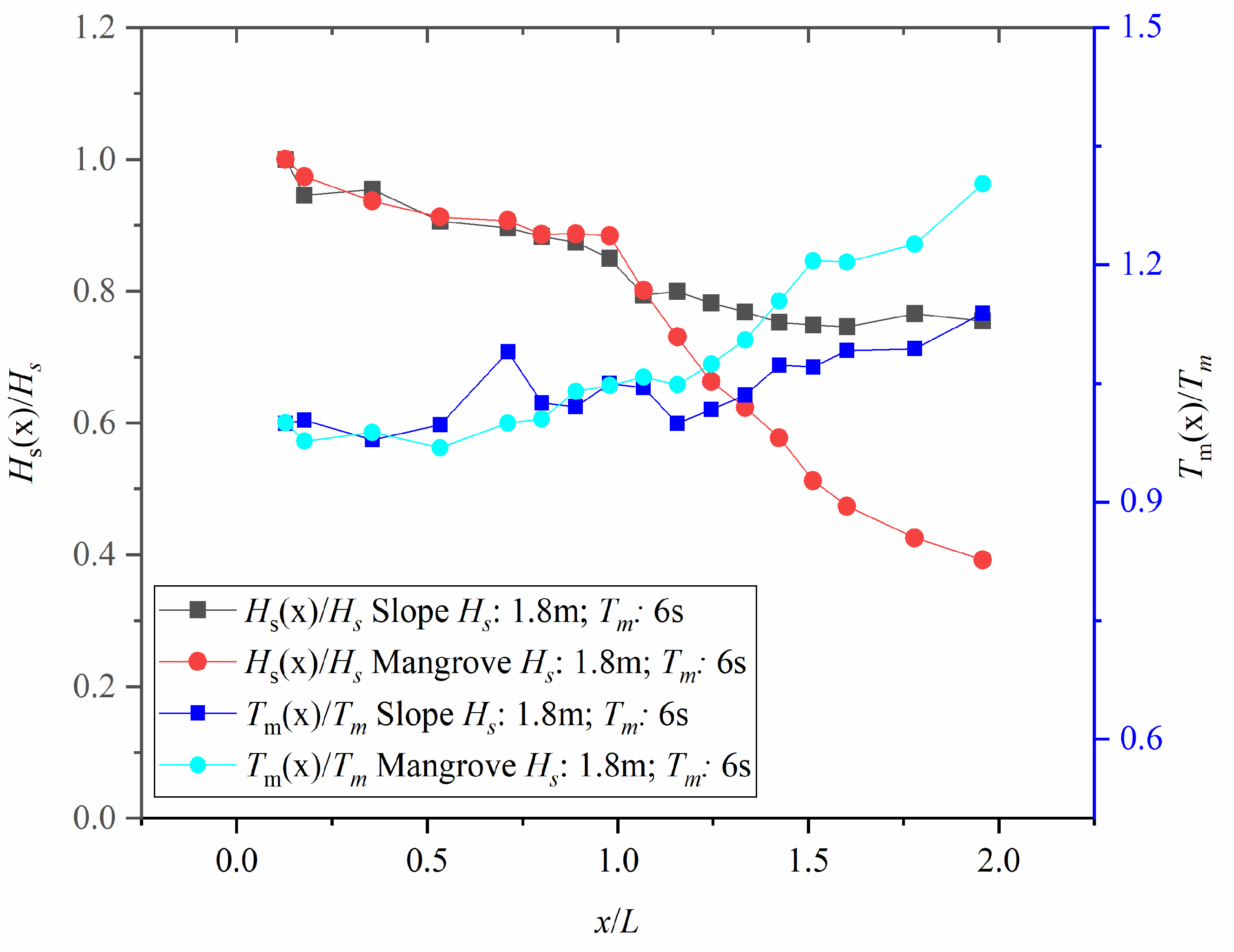
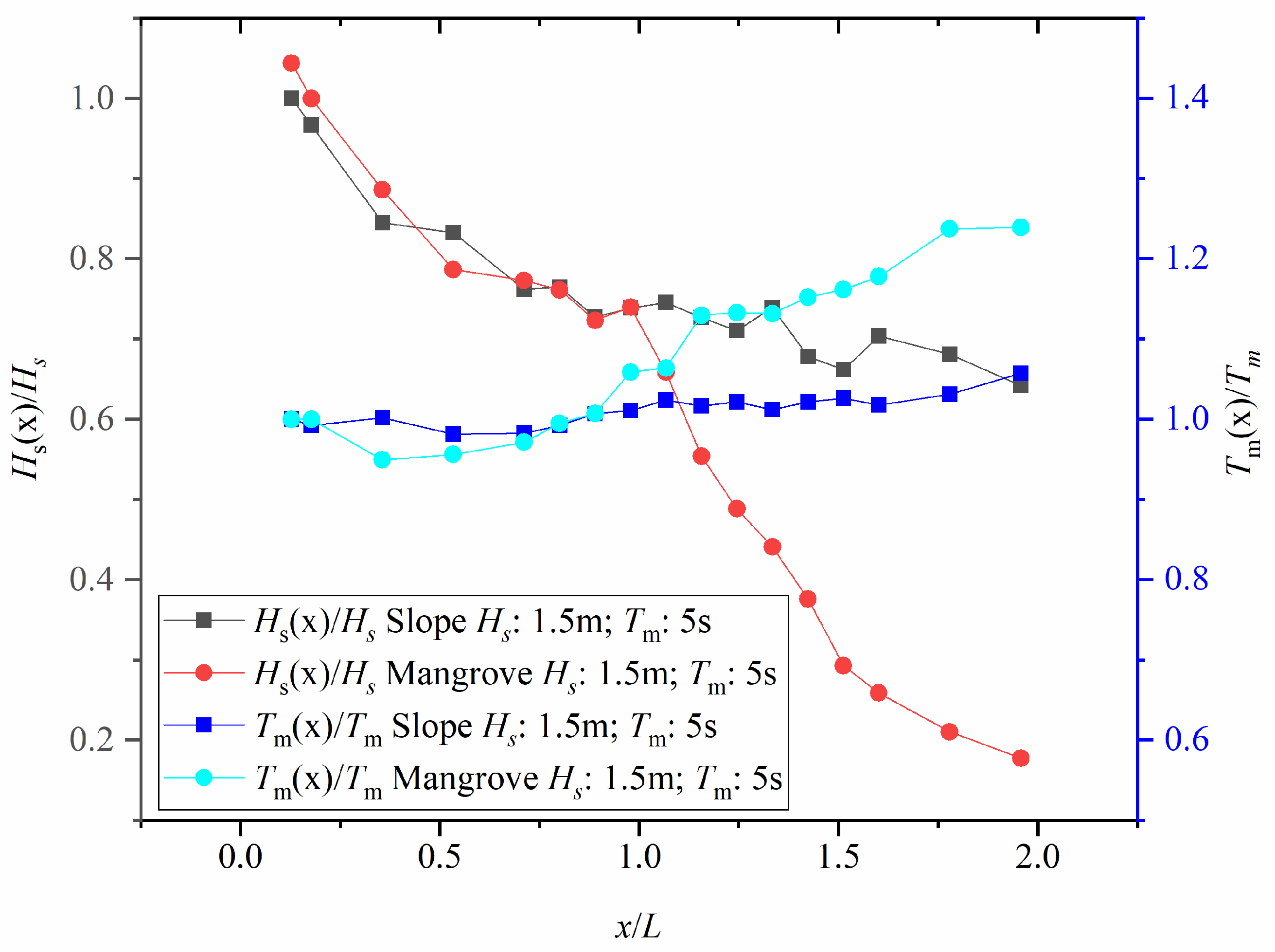
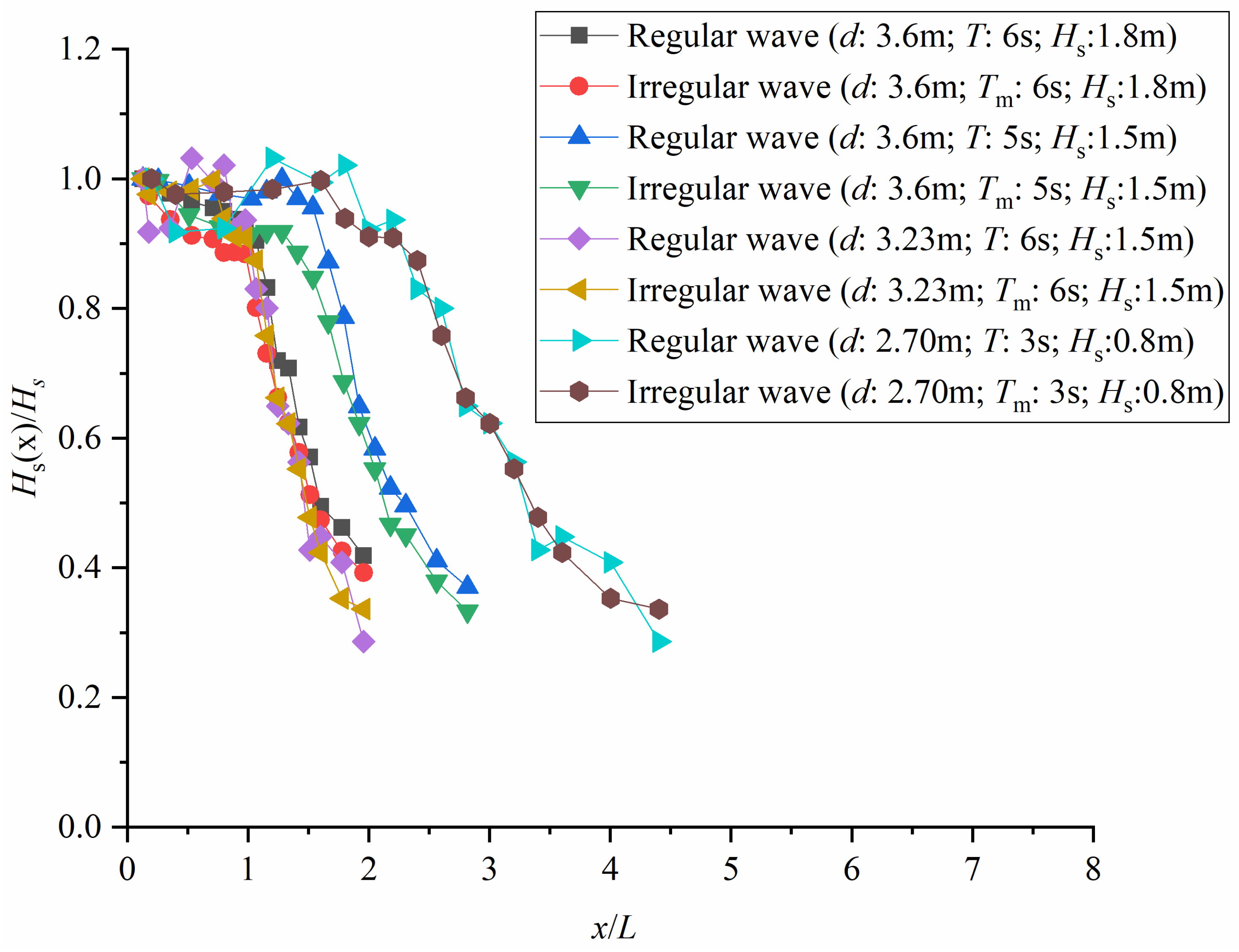
4.1. The Longitudinal Variation in Wave Parameters

The experimental data collected from the wave attenuation studies involving Kandelia obovata are meticulously analyzed using various methods tailored to the specific wave conditions. For the experiments conducted under regular wave conditions, the zero-up crossing method is employed to process the raw time series data obtained from the free surface level measurements. This method helps to determine crucial wave parameters such as the root-mean-square wave height ($H_{rms}$) and mean wave period ($T_m$) at each of the wave gauges positioned within the model forests. For the experiments using irregular waves, the analysis follows a similar approach to that outlined by [17]. The spectral wave characteristics are derived through Fast Fourier Transform (FFT), which transforms the time series data on water elevation into a frequency domain representation. From the spectrum, the spectral wave height ($H_{m0}$) is calculated based on the total energy contained within it and is approximated to be equal to $H_s$. Additionally, $T_m$ is also estimated for irregular wave scenarios. To facilitate comparison between the results from the monochromatic and irregular wave experiments, the spectral moment wave heights are converted into equivalent values under a Rayleigh distribution assumption, where $H_s=H_{m0}=1.416{ H}_{rms}$ by assuming a Rayleigh distribution, as mentioned above.

Taking the shallow water effect into consideration, the time-averaged wave energy flux is defined as [42]:

$$E_T={\displaystyle \sum _{i=1}^{\mathrm{\infty }}}{\displaystyle \frac{1}{8}}\rho g{H}_j^2·{\displaystyle \frac{c_j}{2}}\left(1+{\displaystyle \frac{2k_{j}h}{\sinh \left(2k_{j}h\right)}}\right)$$

(11)

$$K_{EV}=K_{Et}+\left(1-K_{Eb}\right)$$

(12)

where $H_j$ is the wave height of the jth wave by Fourier-based analysis. $c_j$ and $k_j$ are the corresponding wave velocity and wave number. $K_{EV}$ is the wave energy loss due to vegetation only. $K_{Et}$ is the total wave energy loss and $K_{Eb}$ is the wave energy loss caused by shallow water effects, bottom frictional effects, and the boundary effect by the walls of the wave flume. Data collected in the control group and experimental group were used to calculate $K_{Eb}$ and $K_{Et}$, respectively.

$H_s\left(x\right)/H_s$ along the distance axis $x/L$, where $L$ represents the wavelength computed based on $d$ and $T_m$ at the toe of the mild slope (the location of wave gauge G1), is graphically presented in Figure 3, Figure 4 and Figure 5 for different water depths, and all data have been converted to prototype scale through scaling. It is important to emphasize that the $H_s$ depicted in these figures refers to the incident wave height measured at the edge of the sloping area (the location of wave gauge G1), which differs from $H_{s,i}$ (the location of wave gauge G8), which signifies the wave height after passing through the artificial Kandelia obovata forest and is, thus, recorded at the edge of the mangrove area. These graphs serve as visual aids to understand how the wave energy attenuates over a given distance under varying water depths and illustrate the effect of the artificial Kandelia obovata forests on wave attenuation across multiple scenarios. By comparing the attenuation patterns between the control tests without mangroves (denote as Slope) and those with mangroves (denote as Mangrove), the present authors can quantify the effectiveness of the mangrove models in reducing wave energy and assess their potential as a coastal protection measure.

From the data presented in Figure 3, Figure 4 and Figure 5, it can be discerned that, generally, following the passage through the mangrove forest, $T_m\left(x\right)/T_m$ experienced an appreciable increase across both experimental and control groups. In the present experiments, the wave attenuation of high-frequency components was faster than that of low-frequency components, resulting in an increase in $T_m$ (Figure 6). Figure 6 illustrates the results of the Fourier analysis for the data collected by wave gauge G8 and wave gauge G15, demonstrating that, as waves pass through both G8 and G15, there was a noticeable reduction in wave peak frequency. Additionally, $H_j\left(\mathrm{G}15\right)/H_j\left(\mathrm{G}8\right)$ (the ratio of $H_j$ is the wave height of the jth wave by Fourier-based analysis of G15 to that of G8) decreased progressively as the frequency increased. Specifically, at frequencies of 0.25Hz and 2.5 Hz, the relative wave height ratios were 0.55 and 0.179, respectively, indicating that the former was approximately three times that of the latter. This phenomenon is highly consistent with previous work [16,43].

In terms of wave height attenuation, Figure 3, Figure 4 and Figure 5 demonstrate a compelling performance by the artificial Kandelia obovata forests in reducing wave heights under the given experimental settings. A stark contrast can be observed between the $H_s\left(x\right)$ of the control group and that of the experimental group, where $H_s\left(x\right)$ exhibits a marked decline. The extent of $H_s$ attenuation varied according to different wave conditions. Broadly speaking, the ability of Kandelia obovata to attenuate waves height diminished as the water depth ($d$) increased. At the position of G17, when $d$ was equal 2.70 m, $H_s\left(x\right)/H_s$ typically fell within the range from 10% to 20%, indicating a noteworthy reduction in wave height. As $d$ rose to 3.23 m, this ratio escalated at the same location by approximately 25% to 40%. Upon reaching a $d$ of 3.60 m, the wave height attenuation stabilized at around 30% to 40% at G17. It is worth noting that, for a $d$ of 3.23 m and 3.60 m, the wave height attenuation rates were comparably close under these specific experimental circumstances, suggesting a plateau in the attenuation capability of the artificial mangrove forest in deeper water conditions. Indeed, it is essential to acknowledge that wave attenuation is not exclusively attributed to the presence of mangrove forests like Kandelia obovata. Other critical environmental factors, such as alterations in bathymetry, seabed roughness leading to bottom friction, and lateral boundary effects, also contribute substantially to the overall damping of wave energy.

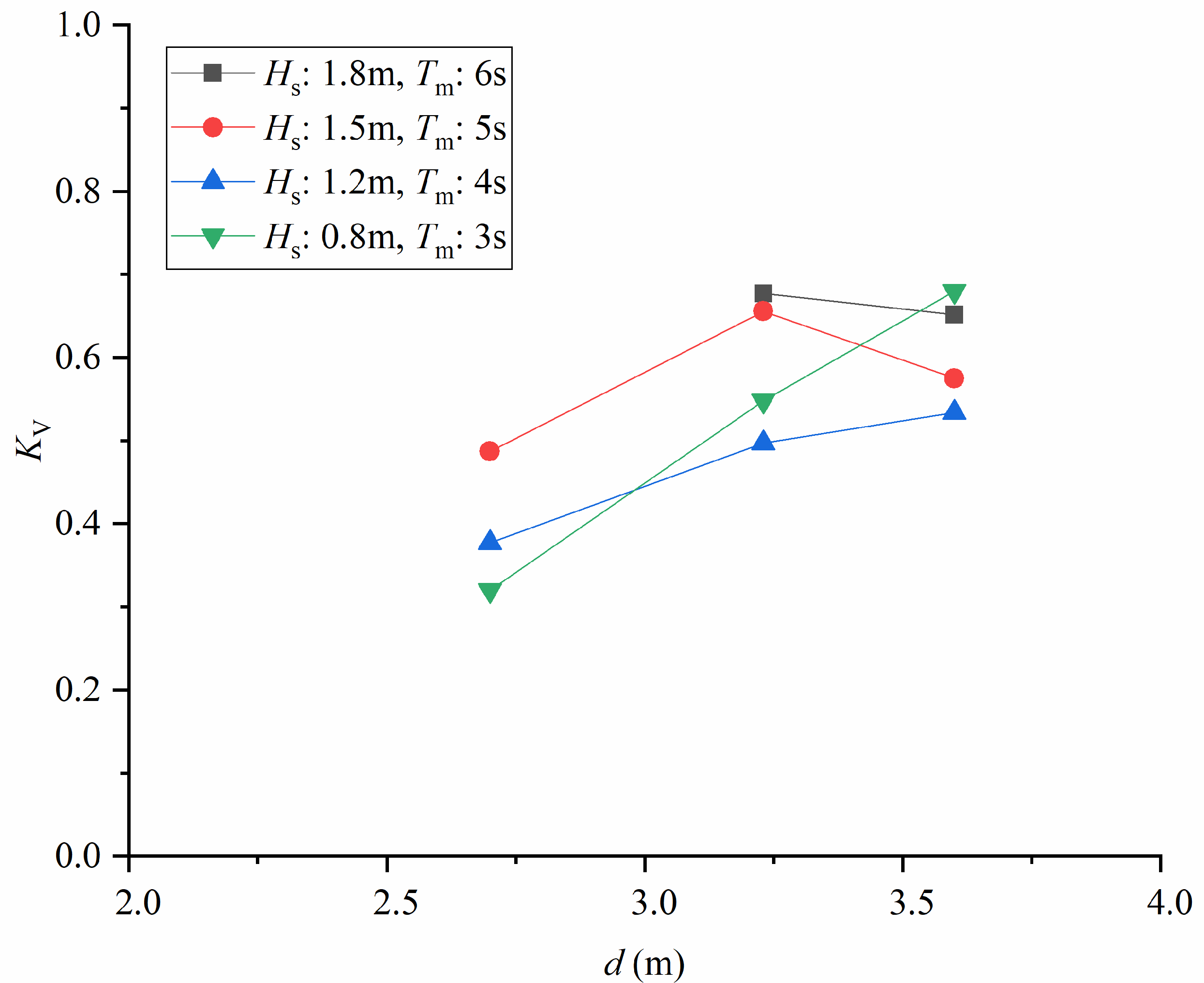
4.2. The Effect of Water Depth on Wave Attenuation

To better elucidate this multifaceted aspect of wave attenuation, Figure 7 presents the effect of $d$ on $K_V$ under consistent wave parameter conditions. This graphic offers a clearer picture of how the effectiveness of Kandelia obovata in attenuating waves interacted with changing water depths, illustrating the interplay between the mangrove forest’s influence and other influencing factors.

Referring to Figure 7, under a constant $H_s$ and $T_m$, upon increasing $d$ from 2.70 m to 3.23 m, the nonlinearity of the waves diminished, thereby reducing wave attenuation and correspondingly leading to an increase in $K_V$. When $d$ further escalated from 3.23 m to 3.60 m, the wave nonlinearity continued to weaken. For the mangrove model composed of cylinder arrays, this increase in water depth typically translated to decreased wave attenuation and a consequent rise in $K_V$, indicating less energy loss through the mangrove model. However, the present study employed a vertically varying model, which includes a canopy section naturally positioned in the region where the wave energy was most concentrated. This design element dramatically enhanced wave attenuation, counteracting the expected decrease in attenuation due to an increased $d$. Thus, despite the deepening water, the wave attenuation significantly increased in several cases, which ultimately resulted in a decrease in $K_V$, demonstrating the effectiveness of the vertical-variation model in enhancing the wave-dampening properties of artificial Kandelia obovata forests, as shown in Figure 7. Moreover, wave attenuation has been found to increase with an increase in the $Ur$, which is a dimensionless quantity that characterizes the relative importance of nonlinear shoaling and refraction effects in shallow water waves. This correlation is consistent with previous research findings [44], reinforcing the understanding that the complexity of wave dynamics, including nonlinear effects, plays a significant role in determining the wave attenuation within the artificial mangrove forest system.

When $d$ is 2.70 m, the shallow water effects on waves are particularly pronounced, where in the controlled experiments of Case. A16–Case. A18, it was observed that $H_s$ did not attenuate as expected but, in fact, exhibited some amplification in the readings from several wave gauges. Thus, Equation (11) is taken to isolate the wave attenuation by artificial Kandelia obovata from other factors.

Regarding the comparative analysis between regular and irregular waves, the outcomes are visually represented in Figure 8. This figure showcases the differences in the wave attenuation performance of the artificial Kandelia obovata forests under identical wave parameters. Regular waves display a consistent frequency and period throughout their propagation, allowing for a straightforward evaluation of wave attenuation over a uniform spectrum. Conversely, irregular waves consist of a continuous distribution of frequencies and periods, providing a more realistic representation of natural wave conditions. In Figure 8, the comparative assessment demonstrates the distinct response of the mangrove forest to these differing wave regimes, highlighting any variations in attenuation efficiency and offering insight into the forest’s ability to mitigate wave energy across a range of wave types.

Generally speaking, the energy dissipation of regular waves exceeded that of irregular waves by about 2–10% of the incident waves (measured by wave gauge G1). But special attention should be paid to a notable phenomenon in the comparison of Case B1 (irregular wave with $H_s$ = 1.8 m, $T_m$ = 6 s, and $d$ = 3.60 m) and Case B5 (regular wave with $H_s$ = 1.8 m, $T_m$ = 6 s, and $d$ = 3.60 m). A probable underlying cause, as inferred from the aforementioned Section 4.1, lay in the differing rates of attenuation among waves with varying periods ($1/f$). Waves with longer periods experience slower attenuation, whereas those with shorter periods attenuate more rapidly. In Case B1, the combination of a larger average wave period and a greater water depth led to a higher proportion and slower attenuation of high-frequency wave energy compared to other experimental groups. Consequently, this scenario gave rise to the unusual instance where regular waves exhibited greater attenuation than irregular ones. The same phenomenon was observed in the comparison of Case B2 (irregular wave with $H_s$ = 1.5 m, $T_m$ = 5 s, and $d$ = 3.60 m) and Case B6 (regular wave with $H_s$ = 1.5 m, $T_m$ = 5 s, and $d$ = 3.60 m).

As demonstrated in Figure 8, both wave types exhibited an increase in $K_V$ as wave nonlinearity increased while keeping the other wave parameters constant. This finding suggests that the artificial Kandelia obovata forests’ attenuation effect was comparable for regular and irregular waves under similar conditions.

4.3. The Effect of Elastic Model with Canopy on Wave Attenuation

By comparing the rigid cylinders model with the rigid cylinders model with a canopy, the influence of using the elastic model with a canopy can be clearly illustrated. Thus, the data of present work are compared with Equation (3) ($K_{\mathrm{V},\mathrm{Z}\mathrm{h}\mathrm{a}\mathrm{n}\mathrm{g}}$, rigid cylinders model) and Equation (4) ($K_{\mathrm{V},\mathrm{H}\mathrm{e}}$, rigid cylinders model with a canopy). It should be noted that, due to the limitations of the applicability of Equation (3) ($0.73<Ur<21.33$), the experiments in this article only compare $Ur$ within this scope. That is, there are eight cases, including Case B1-Case B4 and Case B12–Case B15, plotted in Figure 9.

From Figure 9, it can be seen that Equation (4), using the rigid model with a canopy, had a high degree of agreement with the present experimental values, with the seven predicted values ranging from 80% to 100%. The overall average deviation was 2%, which means that the wave attenuation using the elastic model with a canopy was 2% lower than that using the rigid model with a canopy. However, Equation (3), using a fully rigid cylindrical model, was significantly overestimated with an average deviation of 15%, mainly due to the fact that the wave dissipation effect of the canopy was not taken into account. In general, Equation (4) had a better performance than Equation (3) in the present work. Using an elastic model for simulating the wave attenuation by mangroves showed only minor differences compared with the rigid model, however, employing a model that took into account the canopy of the mangrove trees led to a more significantly increased wave attenuation effect compared to the rigid model. The present experimental results demonstrate that the wave-dissipating function of canopies is notably strong, implying that the influence of canopies should not be overlooked in research on mangrove forests. This phenomenon is consistent with findings from previous research [20,23].

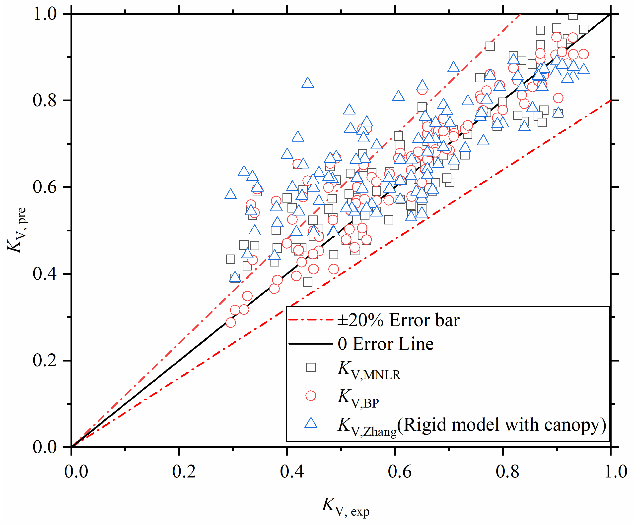
5. Prediction of Wave Transmission and Bulk Drag Coefficient

5.1. Multivariate Nonlinear Regression Method (MNLR)

In the present study, artificial Kandelia obovata forests were systematically modeled to examine the influence of hydrodynamic conditions on wave attenuation. To thoroughly explore the relationship between these experimental conditions and $K_V$, four dimensionless hydrodynamic parameters were chosen as predictors:

Relative Wave Height ($H_r$, the ratio of the wave height to the water depth): This parameter encapsulates the scaled wave height and allows for an assessment of how the magnitude of the waves affects the attenuation through the mangrove forests (Equation (14)). Submerged Ratio ($\alpha$): This factor reflects the portion of the mangrove cylinders that are submerged underwater, accounting for the role of $h$ in wave attenuation. A higher submerged ratio indicates that a larger part of the vegetation interacts with the waves, potentially leading to increased attenuation (Equation (15)). Ursell Number ($Ur$): This dimensionless number is indicative of the significance of nonlinear wave effects, such as shoaling and refraction, in shallow water environments [44]. An increase in $Ur$ suggests stronger nonlinearities, which can affect the wave attenuation in the Kandelia obovata forests (Equation (16)). Relative Width of Kandelia obovata Forests ($B/L$): This ratio measures $B$ relative to $L$, capturing the influence of the spatial extent of the vegetation on wave dissipation [25]. A larger $B/L$ implies that waves interact with a wider stretch of the forest, which could either enhance or limit wave attenuation, depending on the configuration and arrangement of the vegetation.

By analyzing these four predictors in tandem, the study aimed to quantify the individual contributions of each hydrodynamic parameter to the overall wave attenuation, as characterized by $K_V$, thereby gaining a deeper understanding of the underlying mechanisms governing wave energy dissipation in artificial Kandelia obovata forests.

$$H_r(x)={\displaystyle \frac{H_{s,i}\left(x\right)}{d\left(x\right)}}$$

(13)

$$\alpha (x)={\displaystyle \frac{h\left(x\right)}{d\left(x\right)}}$$

(14)

$$Ur(x)={\displaystyle \frac{H_{s,i}{L}^2}{{d\left(x\right)}^3}}$$

(15)

To make Equation (5) dimensionless, substituting Equations (13)–(15) into Equation (5),

$$K_V\left(x\right)=\phi \left(H_r\left(x\right);\alpha \left(x\right);Ur\left(x\right);B/L\right)$$

(16)

To maximize the utilization of the collected experimental data, the dataset was divided and analyzed based on incremental segments of 1.0 m each, ranging from 1.0 m to 5.0 m. This segmentation strategy effectively multiplied the original dataset, expanding it from 21 independent groups to a total of 105 data subsets. Each subset corresponded to the wave characteristics measured at intervals of 1.0 m along the path traversed by the waves through the artificial Kandelia obovata forests, thereby providing a more granular view of wave attenuation and its dependence on distance. This approach enables a comprehensive analysis of how wave parameters such as $H_s$, $T_m$, and others varied with distance and facilitates a more robust understanding of the hydrodynamic processes occurring within the mangrove forest system.

Based on the present experiments, the form of power function was selected, as it has been proven to be suitable for calculating $K_V$ [23,31]. In addition, $K_V$ was used as the dependent variable, and $H_r$, $\alpha$, $Ur$, and $B/L$ were used as independent variables. The least-squares method was used to conduct multivariate nonlinear regression fitting, which is expressed (with a determination coefficient $R^2$ of 0.80) as

$$K_V\left(x\right)={0.742H_r}^{0.247}{\mathsf{\alpha }}^{1.0}{Ur}^{-0.118}{\left({\displaystyle \frac{B}{L}}\right)}^{-0.325}$$

(17)

5.2. Back Propagation (BP) Neural Network Method

In recent years, the application of neural network methods has gained traction in estimating the dissipation of solitary waves due to mangrove forests, as evidenced by studies conducted by [30,31], which demonstrated promising results. Building upon this success, the present study adopted the back propagation (BP) algorithm, a widely used neural network architecture consisting of input, hidden, and output layers, to predict wave attenuation within the context of artificial Kandelia obovata forests. Just like in the multivariate nonlinear regression (MNLR) approach, the experimental data and the selected hydrodynamic parameters in the neural network model remained consistent. These parameters included $H_r$, $\alpha$, $Ur$, and $B/L$. By training the BP neural network with these inputs and corresponding wave attenuation measurements, the model was expected to learn the complex relationships among these variables and accurately predict wave attenuation under various conditions. This approach offers a powerful tool for simulating and predicting the wave-damping capabilities of mangrove ecosystems, which is crucial for coastal protection and habitat restoration efforts. The experimental data of the present study are divided into training, validation, and testing sets in a ratio of 75:15:15 to avoid under-fitting and overfitting. The number of neurons in the hidden layer of a neural network is commonly estimated using empirical formulas such as Equations (17) and (18) [31], which provide a range of suitable neuron counts based on the complexity of the problem and available data.

$$n_{\mathrm{h}}=\sqrt{n_{\mathrm{I}}+n_{\mathrm{O}}}+a$$

(18)

$$M<\sum _{i=0}^{n_I}{C}_{n_{\mathrm{h}}}^i$$

(19)

where, $n_{\mathrm{I}}$, $n_{\mathrm{O}}$, and $n_{\mathrm{h}}$ denote the numbers of neurons in the input, output, and hidden layers, respectively. The constant $a$ ranges between 1 and 10, and $M$ represents the total number of training samples. Importantly, when $i$ > $n_{\mathrm{h}}$, $C_{n_{\mathrm{h}}}^i$ is set to 0.

In the current research project, determining the ideal number of neurons in the hidden layer involves experimenting with different configurations of the BP neural network and selecting the setup that achieves the lowest root-mean-square error (RMSE). This process ensured that the model’s predictions were as accurate as possible under the various wave scenarios. To minimize the influence of random initial weight assignments and potential threshold effects that could impact the predicted outcomes, the BP model was executed ten times for each wave condition.

The present work reveals that the optimal number of neurons in the hidden layer is seven, which minimizes the RMSE and, thus, maximizes the accuracy of wave attenuation predictions. For comparative analysis, the study also examines Equation (4) employed by [20]. In Figure 10, $K_{\mathrm{V},\mathrm{M}\mathrm{N}\mathrm{L}\mathrm{R}}$, $K_{\mathrm{V},\mathrm{B}\mathrm{P}}$, and $K_{\mathrm{V},\mathrm{Z}\mathrm{h}\mathrm{a}\mathrm{n}\mathrm{g}}$ refer to the values of $K_{\mathrm{V}}$ calculated using the MNLR method, the BP neural network, and Equation (4), respectively. These values are then compared against the experimental values $K_{\mathrm{V},\mathrm{e}\mathrm{x}\mathrm{p}}$.

From Figure 10, it is evident that $K_{\mathrm{V},\mathrm{Z}\mathrm{h}\mathrm{a}\mathrm{n}\mathrm{g}}$ consistently overestimated $K_V$ by approximately 30% when $K_{\mathrm{V},\mathrm{e}\mathrm{x}\mathrm{p}}$ was in the scope of 0.3–0.4. This overestimation can primarily be attributed to the short width (2 m) of the mangrove in their experiment [20]. A narrower width in the mangrove model would lead to calculated $K_V$ values that cannot be directly extrapolated to wider mangrove scenarios. Consequently, Equation (4) performed better in prediction when $K_V$ was larger (corresponding to narrower mangrove widths); however, it exhibited greater prediction errors when $K_V$ was smaller (indicating larger actual mangrove widths). Figure 10 illustrates that the BP method delivered the best prediction performance, as over 90% of the data points fell within a 20% error margin when compared to the experimental values. This indicates that the BP neural network model was highly effective in approximating the wave attenuation through artificial Kandelia obovata forests, outperforming both the MNLR method and the method of [20] in terms of prediction accuracy.

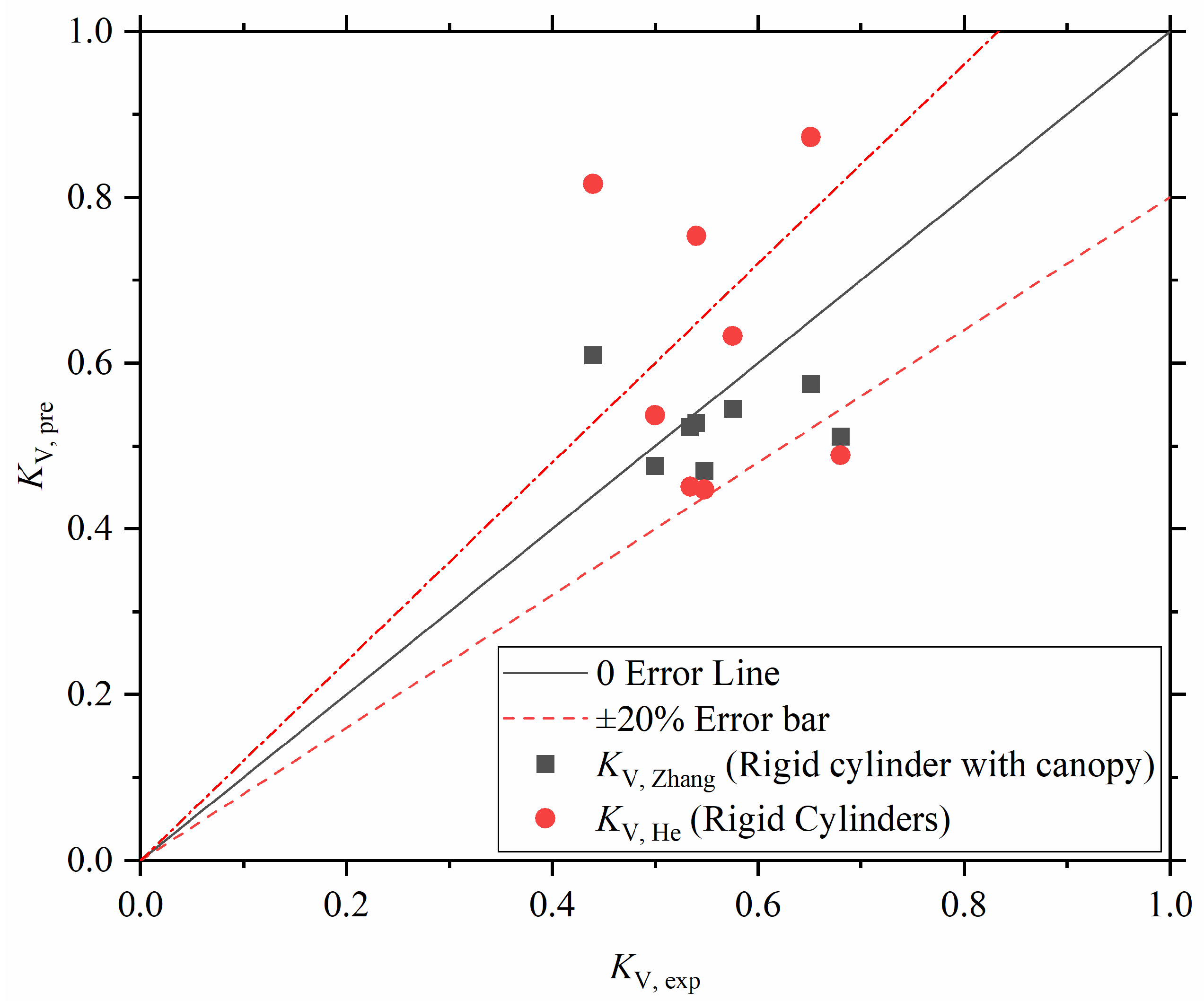
5.3. Bulk Drag Coefficient

In present work, $C_D$ can be calculated by the Equations (1) and (2) [32]. Previous works have shown the relationship between $C_D$ and dimensionless parameters [20,21,23,26,31]. In light of the considerable agreement observed between Equation (4) and the current experimental results, it was decided to improve Equation (4) to enhance its applicability to the present study. The improved equation is given as below (with a determination coefficient $R^2$ of 0.82):

$$C_D=0.60+{\left({\displaystyle \frac{18.7}{Ur}}\right)}^{1.11}$$

(20)

According to the present work, $Ur$ was in the scope of 2.6–72. A comparison between the measured and predicted $C_D$ (both Equations (4) and (20) are taken for prediction) for the present work is illustrated in detail in Figure 11. Due to the complexity of wave attenuation mechanisms by vegetation, both Equations (4) and (20) led to substantial deviations. Further advancements in the relevant theories necessitate a more comprehensive collection of experimental data and field measurements. It need to be clarified that the present works were deduced in a laboratory study, which may have underestimated the $C_D$ compared with the prototype [40].

6. Conclusions

The present study evaluated wave attenuation by artificial Kandelia obovata forests using a wave flume equipped with effective wave-absorbing technology. $K_V$ was deduced based on the present experiments. Later, the MNLR method, BP neural network, and methods from the previous literature were compared with the present experiments. From the previous discussion, the following conclusions can be drawn: the flexible Kandelia obovata models showed a good performance in wave attenuation under the present experimental conditions, and as the water depth increased from 2.70 m to 3.23 m, the wave nonlinearity and attenuation decreased. However, when the water depth further increased to 3.60 m, the wave attenuation effect by the mangrove forest intensified due to the concentration of wave energy near the canopy area. High-frequency components tended to attenuate faster than the low-frequency parts in present study. Under identical wave parameters, the wave attenuation characteristics for regular and irregular waves were quite similar. The study also revealed that using the elastic model exhibited an average difference of 2% in $K_V$ compared to the rigid model, and neglecting the canopy in the models resulted in an underestimation of $K_V$ by approximately 15% as opposed to considering its presence. Among the predictive methods, the BP neural network method showed the best prediction performance compared with the MNLR and He methods.

References

1. Weaver, R.J.; Stehno, A.L. Mangroves as Coastal Protection for Restoring Low-Energy Waterfront Property. J. Mar. Sci. Eng. 2024, 12, 470. [Google Scholar] [CrossRef]
2. Zeng, J.; Ai, B.; Jian, Z.; Ye, M.; Zhao, J.; Sun, S. Analysis of mangrove dynamics and its protection effect in the Guangdong-Hong Kong-Macao Coastal Area based on the Google Earth Engine platform. Front. Mar. Sci. 2023, 10, 1170587. [Google Scholar] [CrossRef]
3. Zhang, X.; Lin, P.; Chen, X. Coastal protection by planted mangrove forest during typhoon Mangkhut. J. Mar. Sci. Eng. 2022, 10, 1288. [Google Scholar] [CrossRef]
4. Gijsman, R.; Horstman, E.M.; van der Wal, D.; Friess, D.A.; Swales, A.; Wijnberg, K.M. Nature-Based Engineering: A Review on Reducing Coastal Flood Risk with Mangroves. Front. Mar. Sci. 2021, 8, 702412. [Google Scholar] [CrossRef]
5. Alongi, D.M. Mangrove forests: Resilience, protection from tsunamis, and responses to global climate change. Estuar. Coast. Shelf Sci. 2008, 76, 1–13. [Google Scholar] [CrossRef]
6. Quartel, S.; Kroon, A.; Augustinus, P.G.E.F.; Van Santen, P.; Tri, N.H. Wave attenuation in coastal mangroves in the Red River Delta, Vietnam. J. Asian Earth Sci. 2007, 29, 576–584. [Google Scholar] [CrossRef]
7. Mazda, Y.; Magi, M.; Kogo, M.; Hong, P.N. Mangroves as a coastal protection from waves in the Tong King delta, Vietnam. Mangroves Salt Marshes 1997, 1, 127–135. [Google Scholar] [CrossRef]
8. Zhao, C.; Tang, J.; Shen, Y. Numerical investigation of the effects of rigid emergent vegetation on wave runup and overtopping. Ocean Eng. 2022, 264, 112502. [Google Scholar] [CrossRef]
9. Borsje, B.W.; van Wesenbeeck, B.K.; Dekker, F.; Paalvast, P.; Bouma, T.J.; van Katwijk, M.M.; de Vries, M.B. How ecological engineering can serve in coastal protection. Ecol. Eng. 2011, 37, 113–122. [Google Scholar] [CrossRef]
10. Ren, H.; Lu, H.; Shen, W.; Huang, C.; Guo, Q.; Li, Z.a.; Jian, S. Sonneratia apetala Buch.Ham in the mangrove ecosystems of China: An invasive species or restoration species? Ecol. Eng. 2009, 35, 1243–1248. [Google Scholar] [CrossRef]
11. Mullarney, J.C.; Henderson, S.M.; Reyns, J.A.H.; Norris, B.K.; Bryan, K.R. Spatially varying drag within a wave-exposed mangrove forest and on the adjacent tidal flat. Cont. Shelf Res. 2017, 147, 102–113. [Google Scholar] [CrossRef]
12. Mazda, Y.; Magi, M.; Ikeda, Y.; Kurokawa, T.; Asano, T. Wave reduction in a mangrove forest dominated by Sonneratia sp. Wetl. Ecol. Manag. 2006, 14, 365–378. [Google Scholar] [CrossRef]
13. Horstman, E.M.; Dohmen-Janssen, C.M.; Narra, P.M.F.; van den Berg, N.J.F.; Siemerink, M.; Hulscher, S.J.M.H. Wave attenuation in mangroves: A quantitative approach to field observations. Coast. Eng. 2014, 94, 47–62. [Google Scholar] [CrossRef]
14. Vo-Luong, P.; Massel, S. Energy dissipation in non-uniform mangrove forests of arbitrary depth. J. Mar. Syst. 2008, 74, 603–622. [Google Scholar] [CrossRef]
15. Brinkman, R.M.; Massel, S.R.; Ridd, P.V.; Furukawa, K. Surface Wave Attenuation in Mangrove Forests. In Proceedings of the Pacific Coasts and Ports ’97: Proceedings of the 13th Australasian Coastal and Ocean Engineering Conference and the 6th Australasian Port and Harbour Conference, Christchurch, New Zealand, 7–11 September 1997; Volume 2. [Google Scholar]
16. Wu, W.-C.; Cox, D.T. Effects of wave steepness and relative water depth on wave attenuation by emergent vegetation. Estuar. Coast. Shelf Sci. 2015, 164, 443–450. [Google Scholar] [CrossRef]
17. Augustin, L.N.; Irish, J.L.; Lynett, P. Laboratory and numerical studies of wave damping by emergent and near-emergent wetland vegetation. Coast. Eng. 2009, 56, 332–340. [Google Scholar] [CrossRef]
18. Bouma, T.J.; De Vries, M.B.; Low, E.; Peralta, G.; Tánczos, I.C.; van de Koppel, J.; Herman, P.M.J. Trade-Offs Related to Ecosystem Engineering: A Case Study on Stiffness of Emerging Macrophytes. Ecology 2005, 86, 2187–2199. [Google Scholar] [CrossRef]
19. van Veelen, T.J.; Fairchild, T.P.; Reeve, D.E.; Karunarathna, H. Experimental study on vegetation flexibility as control parameter for wave damping and velocity structure. Coast. Eng. 2020, 157, 103648. [Google Scholar] [CrossRef]
20. Zhang, R.; Chen, Y.; Lei, J.; Zhou, X.; Yao, P.; Stive, M.J.F. Experimental investigation of wave attenuation by mangrove forests with submerged canopies. Coast. Eng. 2023, 186, 104403. [Google Scholar] [CrossRef]
21. Wang, Y.; Yin, Z.; Liu, Y. Experimental investigation of wave attenuation and bulk drag coefficient in mangrove forest with complex root morphology. Appl. Ocean Res. 2022, 118, 102974. [Google Scholar] [CrossRef]
22. Piedrahita, M.; Osorio, A.; Urrego, L.; Gallego, J.D. Study of the Velocity and Wave Damping in a Physical Model of a Mangrove Forest Including Secondary Roots. In Proceedings of the Coastal Structures, Hannover, Germany, 29 September–2 October 2019; Bundesanstalt für Wasserbau: Karlsruhe, Germany, 2019. [Google Scholar]
23. He, F.; Chen, J.; Jiang, C. Surface wave attenuation by vegetation with the stem, root and canopy. Coast. Eng. 2019, 152, 103509. [Google Scholar] [CrossRef]
24. Sha, L.; Ming, C.; Gangfeng, M.; Shuguang, L.; Guihui, Z. Laboratory study of the effect of vertically varying vegetation density on waves, currents and wave-current interactions. Appl. Ocean Res. 2018, 79, 74–87. [Google Scholar] [CrossRef]
25. Hashim, A.M.; Catherine, S.M.P. A Laboratory Study on Wave Reduction by Mangrove Forests. APCBEE Procedia 2013, 5, 27–32. [Google Scholar] [CrossRef]
26. Kelty, K.; Tomiczek, T.; Cox, D.T.; Lomonaco, P.; Mitchell, W. Prototype-Scale Physical Model of Wave Attenuation through a Mangrove Forest of Moderate Cross-Shore Thickness: LiDAR-Based Characterization and Reynolds Scaling for Engineering with Nature. Front. Mar. Sci. 2022, 8, 780946. [Google Scholar] [CrossRef]
27. Chang, C.W.; Mori, N.; Tsuruta, N.; Suzuki, K.; Yanagisawa, H. An Experimental Study of Mangrove-Induced Resistance on Water Waves Considering the Impacts of Typical Rhizophora Roots. J. Geophys. Res. Ocean. 2022, 127, e2022JC018653. [Google Scholar] [CrossRef]
28. Maza, M.; Lara, J.L.; Losada, I.J. Experimental analysis of wave attenuation and drag forces in a realistic fringe Rhizophora mangrove forest. Adv. Water Resour. 2019, 131, 103376. [Google Scholar] [CrossRef]
29. Strusińska-Correia, A.; Husrin, S.; Oumeraci, H. Tsunami damping by mangrove forest: A laboratory study using parameterized trees. Nat. Hazards Earth Syst. Sci. 2013, 13, 483–503. [Google Scholar] [CrossRef]
30. Malvin, N.; Pudjaprasetya, S.R.; Adytia, D. Neural Network Modelling on Wave Dissipation Due to Mangrove Forest. In Proceedings of the 2020 International Conference on Data Science and Its Applications (ICoDSA), Bandung, Indonesia, 5–6 August 2020; pp. 1–7. [Google Scholar]
31. Yin, Z.; Li, J.; Wang, Y.; Wang, H.; Yin, T. Solitary wave attenuation characteristics of mangroves and multi-parameter prediction model. Ocean Eng. 2023, 285, 115372. [Google Scholar] [CrossRef]
32. Dalrymple, R.A.; Kirby, J.T.; Hwang, P.A. Wave Diffraction Due to Areas of Energy Dissipation. J. Waterw. Port Coast. Ocean Eng. 1984, 110, 67–79. [Google Scholar] [CrossRef]
33. Mendez, F.J.; Losada, I.J. An empirical model to estimate the propagation of random breaking and nonbreaking waves over vegetation fields. Coast. Eng. 2004, 51, 103–118. [Google Scholar] [CrossRef]
34. Maza, M.; Adler, K.; Ramos, D.; Garcia, A.M.; Nepf, H. Velocity and Drag Evolution from the Leading Edge of a Model Mangrove Forest. J. Geophys. Res. Ocean. 2017, 122, 9144–9159. [Google Scholar] [CrossRef]
35. Bryant, M.; Bryant, D.; Provost, L.; Hurst, N.; McHugh, M.; Wargula, A.; Tomiczek, T. Wave Attenuation of Coastal Mangroves at a Near-Prototype Scale; US Army Engineer Research and Development Center (ERDC): Vicksburg, MS, USA, 2022. [Google Scholar]
36. Cheng, N.S.; Nguyen, H.T. Hydraulic Radius for Evaluating Resistance Induced by Simulated Emergent Vegetation in Open-Channel Flows. J. Hydraul. Eng. 2011, 137, 995–1004. [Google Scholar] [CrossRef]
37. Tinoco, R.O.; Goldstein, E.B.; Coco, G. A data-driven approach to develop physically sound predictors: Application to depth-averaged velocities on flows through submerged arrays of rigid cylinders. Water Resour. Res. 2015, 51, 1247–1263. [Google Scholar] [CrossRef]
38. Hu, Z.; Suzuki, T.; Zitman, T.; Uittewaal, W.; Stive, M. Laboratory study on wave dissipation by vegetation in combined current–wave flow. Coast. Eng. 2014, 88, 131–142. [Google Scholar] [CrossRef]
39. Booij, N.; Holthuijsen, L.; Ris, R. The” SWAN” wave model for shallow water. In Proceedings of the Coastal Engineering 1996, Orlando, FL, USA, 2–6 September 1996; pp. 668–676. [Google Scholar]
40. Kalloe, S.A.; Hofland, B.; Van Wesenbeeck, B.K. Scaled versus real-scale tests: Identifying scale and model errors in wave damping through woody vegetation. Ecol. Eng. 2024, 202, 107241. [Google Scholar] [CrossRef]
41. Reimann, S.; Husrin, S.; Strusińska, A.; Oumeraci, H. Damping Tsunami And Storm Waves By Coastal Forests—Parameterisation And Hydraulic Model Tests. In Proceedings of the FZK-Kolloquium “Potenziale für die Maritime Wirtschaft”, Hannover, Germany, 26 March 2009. [Google Scholar]
42. Goda, Y. Random Seas and Design of Maritime Structures; World Scientific Publishing Company: Singapore, 2010; Volume 33. [Google Scholar]
43. Foster-Martinez, M.R.; Lacy, J.R.; Ferner, M.C.; Variano, E.A. Wave attenuation across a tidal marsh in San Francisco Bay. Coast. Eng. 2018, 136, 26–40. [Google Scholar] [CrossRef]
44. Phan, K.L.; Stive, M.J.F.; Zijlema, M.; Truong, H.S.; Aarninkhof, S.G.J. The effects of wave non-linearity on wave attenuation by vegetation. Coast. Eng. 2019, 147, 63–74. [Google Scholar] [CrossRef]
Figure 1. The schematic flume configuration and instrument deployment (Not drawn to scale).
Jmse 12 01198 g001
Figure 2. The comparison of Kandelia obovata in field and laboratory. (a) Planted Kandelia obovata in Yueqing City; (b) assembling Kandelia obovata model; (c) the flume with mangrove model; (d) mangrove model used in present experiments; (e) the horizontal layout of the mangrove model; and (f) diagram of the mangrove model experiment.
Jmse 12 01198 g002
Figure 3. The longitudinal variation in H s ( x ) / H s and T m ( x ) / T m with d = 3.60 m.
Jmse 12 01198 g003
Figure 4. The longitudinal variation in H s ( x ) / H s and T m ( x ) / T m with d = 3.23 m.
Jmse 12 01198 g004
Figure 5. The longitudinal variation in H s ( x ) / H s and T m ( x ) / T m with d = 2.70 m.
Jmse 12 01198 g005
Figure 6. The comparison of amplitude spectrum and peak wave period in G8 and G15 in Case B1 ( H s = 1.8 m, T m = 6 s and d = 3.60 m).
Jmse 12 01198 g006
Figure 7. The effect of h on K V with the same wave parameter conditions.
Jmse 12 01198 g007
Figure 8. The comparison of wave attenuation by regular waves and irregular waves.
Jmse 12 01198 g008
Figure 9. The comparison of present experimental results with Equations (3) and (4).
Jmse 12 01198 g009
Figure 10. The comparison of MNLR, Zhang, and BP neural network method.
Jmse 12 01198 g010
Figure 11. The comparison of the measured and predicted C D (with Equations (4) and (20)).
Jmse 12 01198 g011