Abstract
Maritime UAV path planning is a key link in realizing the intelligence of maritime emergency transportation, providing key support for fast and flexible maritime accident disposal and emergency material supply. However, most of the current UAV path planning methods are designed for land environments and lack the ability to cope with complex marine environments. In order to achieve effective path planning for UAV in marine environments, this paper proposes a Directional Drive-Rotation Invariant Quadratic Interpolation White Shark Optimization algorithm (DD-RQIWSO). First, the directional guidance of speed is realized through a directional update strategy based on the fitness value ordering, which improves the speed of individuals approaching the optimal solution. Second, a rotation-invariant update mechanism based on hyperspheres is added to overcome the tracking pause phenomenon in WSO. In addition, the quadratic interpolation strategy is added to enhance the utilization of local information by the algorithm. Then, a wind simulation environment based on the Lamb–Oseen vortex model was constructed to better simulate the real scenario. Finally, DD-RQIWSO was subjected to a series of tests in 2D and 3D scenarios, respectively. The results show that DD-RQIWSO is able to realize path planning under wind environments more accurately and stably.
1. Introduction
In contemporary times, the application scope of unmanned aerial vehicles (UAVs), which are a kind of controllable vehicle that performs various tasks without human assistance [1], is progressively diversifying, exhibiting significant potential and advantages across various domains such as transportation [2] and construction [3]. With continuous technological advancements, UAVs have emerged as versatile tools for civilian and commercial applications [4]. The marine environment is complex and varied, and compared to the study of the land environment, the marine scene has a rich and diverse range of research scenarios [5,6,7,8], such as marine transportation [9], marine monitoring [10] and other fields [11,12]. Among them, the research on marine transportation has become one of the hot spots of marine research. In maritime environments, there may arise situations necessitating urgent material supply, for which a device capable of swift response and delivery is required. Compared to traditional lifeboats and life rafts, UAVs offer lower time and economic costs and broader transportation coverage, and thus are more conducive to the transportation of materials in maritime emergencies.
Path planning is a critical issue within the field of automation [13], and for UAVs, solving their path planning problems holds considerable value in their applications. Path planning is inherently a combinatorial optimization problem, tasked with generating a geometric path without any specified time constraints. The objective of path planning is to devise a feasible route that ensures safe arrival at the destination based on known environmental information. Its definition is succinct: “find a collision-free motion between an initial (start) and a final configuration (goal) within a specified environment” [13]. Research shows that the path planning problem is an NP-hard problem [14], which means this problem entails large search spaces, making it exceedingly difficult to find the optimum. Solutions to this problem often necessitate exhaustive exploration of numerous possibilities, without any efficient method guaranteeing the discovery of the optimal solution within polynomial time. Consequently, while it may be straightforward to verify whether a given solution is correct, finding a solution itself is highly challenging [15].
Various algorithms, such as A* [16], RRT [17] and PRM [18], are proposed to solve the path planning problem and obtain a feasible solution. As the complexity of the problem to be solved increases, many such improved algorithms have been proposed and applied. For instance, the LDA* algorithm is proposed to finish the path planning mission in a game by Bayili et al. [19] and Moon et al. use a modified RRT algorithm to accomplish the high-speed navigation for mobile robots [20]. However, traditional path planning algorithms typically depend on pre-acquiring and memorizing the global environment graph. These cause an inherent disadvantage of this kind of algorithm. It is time-consuming to use such algorithms for path planning in intricate environments.
Swarm intelligence algorithms mimic swarm behaviors observed in nature to develop intelligent algorithms. Guided by these behaviors, they strategically employ random operators to optimize the trial-and-error process, replicating the exploration of solution spaces based on swarm wisdom. Different from common meta-heuristic algorithms, individuals in swarm intelligence algorithms exhibit independent intelligence and behavior, while enhanced information exchange among the population bolsters the optimization capability. These characteristics empower swarm intelligence algorithms to effectively address complex optimization problems. For example, El-Kenawy et al. propose the hybrid gray wolf optimizer (GWO) and particle swarm optimization (PSO) algorithms to select the best set of features [21]. Mei et al. used an improved meta-heuristic algorithm to enhance the accuracy of target localization in underwater IoT tasks [22]. Mohamed Abdel-Basset modifies the whale optimization algorithm (WOA) to tackle the issue of multi-level thresholding color image segmentation [23]. Given the excellent properties of swarm intelligence algorithms, there are numerous studies that apply swarm intelligence algorithms to path planning [24,25]. The utilization of a modified particle swarm optimization in the path planning of robots has been investigated by Li et al. [26], demonstrating its effectiveness in addressing the path-planning problem. Zhang et al. applied particle swarm optimization to multi-objective path planning, showcasing its potential in the path-planning problem. Zhu proposed an enhanced meta-heuristic algorithm to address the unmanned combat aerial vehicle (UCAV) path planning [27], and Niu et al. solved three-dimensional UCAV path planning in maritime environment with a modified artificial ecosystem optimizer [28], illustrating the feasibility of applying swarm intelligence algorithms to UAV path planning.
Path planning stands as a critical technology ensuring the safety of UAVs in maritime emergency transportation. In maritime environments, path planning for unmanned devices necessitates consideration of marine environmental factors, as well as fuel consumption and obstacle avoidance. For instance, during autonomous underwater vehicle (AUV) path planning in the seafloor environment, factors such as ocean currents and seabed topography are taken into account [29,30]. While UAVs do not require accounting for ocean currents akin to AUV, the impact of marine winds on UAVs cannot be disregarded.
Although numerous swarm intelligence algorithms have been applied to path planning, as described in the “No Free Lunch (NFL)” theorem [31], no single algorithm can tackle all optimization issues. Consequently, exploring novel algorithms to tackle path planning challenges remains a valuable avenue of research, particularly given the increasing complexity of application scenarios and problems. In recent years, several advanced swarm intelligence algorithms have been proposed, including the mayfly algorithm (MA) [32], reptile search algorithm (RSA) [33], beluga whale optimization (BWO) [34] and white shark optimizer (WSO) [35], etc. Among these, WSO stands out as an exemplary swarm intelligence algorithm, which effectively balances the exploration and exploitation processes, and also has excellent performance in some high-dimensional complex test problems, which can effectively detect the search space and converge to the optimal solution to some extent [35]. The existing literature has shown that the WSO algorithm can be applied to the path planning problem and has a great potential [36]. What is more, the WSO algorithm has successfully addressed numerous different types of problems such as optimal power flow problems [37,38], cloud computing [39] and the performance of the design parameters of proton exchange membrane fuel cells (PEMFCs) [40]. When integrated with other strategies, WSO demonstrates capability in resolving more intricate problems. For instance, Ravishankar et al. applied WSO combined with deep learning to solve the problem of UAVs communication and scene classification [41], and Houssein et al. use a modified WSO to solve engineering design and combinatorial problems [42].
The core concepts and inspiration behind the WSO are derived from the behavior of sharks to track prey. This creature possesses remarkable sensory abilities, encompassing their extraordinary auditory, visual and olfactory capabilities. The WSO’s design incorporates a promising blend of exploratory and exploitative search strategies within its update mechanism, achieved through stochastic updates and alterations of solutions. This behavior is modeled in conjunction with the appropriately defined conditions of white shark locomotion and olfactory intensity to foster exploratory behavior in the initial iterations of WSO and exploitative search mechanisms in subsequent iterations.
However, the complexity of problems in the maritime environment, exacerbated by the influence of complex sea winds, imposes higher demands on optimization algorithms, necessitating an enhancement in the search capabilities of WSO populations. There are still some places where WSO can be improved. For instance, in guiding the velocity using individual recorded best values, WSO relies entirely on random individuals, which may not fully exploit the information from individual records, particularly for individuals with less favorable results that warrant stronger optimization behavior. During the fish schooling stage, if the white shark’s visual abilities are insufficient to track the optimal fish, it remains stationary, resulting in missed opportunities to exploit the solution space.
In order to better address path planning problems for UAV maritime emergency transportation, this paper proposes an improved version of the WSO algorithm, named Directional Driven-Rotational Invariant Quadratic Interpolation White Shark Optimizer (DD-RQIWSO), which addresses the aforementioned issues. To accurately simulate the maritime environment, we augment the UAV environment model [43,44] used by Selcuk Aslan and Y. Niu with factors such as sea winds, thus rendering the environment model more representative of real transportation scenarios. The contributions of this paper can be summarized as follows:
- Through the directed update strategy based on sorted cost, the velocity update process of WSO is modified to prevent the degradation phenomenon induced by random individuals, thereby achieving the rapid search capability of directed guidance algorithms;
- An additional rotation-invariant position update mechanism based on hyperspheres is introduced to supplement new individual update patterns, thus avoiding tracking pauses during WSO position updates;
- A quadratic interpolation mechanism is incorporated into WSO to enhance inter-individual information exchange and improve the algorithm’s utilization of local information in complex spaces;
- To simulate real oceanic scenarios, 2D and 3D wind simulation environments based on the Lamb–Oseen vortex model are constructed. A series of tests are conducted on DD-RQIWSO to demonstrate the superiority of the algorithm.
The next part of this paper is structured as follows: The problem formulation of UAV path planning is demonstrated in Section 2. The basic WSO algorithm is displayed in Section 3. The description of the proposed DD-RQIWSO will be shown in Section 4. To inspect the performance of the modified WSO, a series of experimental results are shown in Section 5. Section 6 provides a conclusion of this work.
2. Problem Formulation
Path planning for maritime emergency transportation endeavors to derive an optimal or near-optimal flight route, mitigating risks posed by the intricate maritime environment, including strong electromagnetic interference and the presence of restricted areas of navigation or other areas the UAV cannot fly. Entrance into these areas by a UAV can lead to loss of communication or damage, thus necessitating the designation of no-fly zones within the environment. Fuel consumption emerges as a critical factor influencing UAV flight, primarily dictated by factors such as flight distance and flight smoothness. Wind at sea also impacts fuel consumption and harbors the potential to compromise UAV safety. Consequently, all threat areas and restricted areas of navigation are delineated as no-fly zones. UAVs are instructed to maintain a minimum altitude above sea level, adhere to minimum distance and corner constraints and leverage wind conditions to optimize flight efficiency and safety.
2.1. Modeling of UAV Path Planning
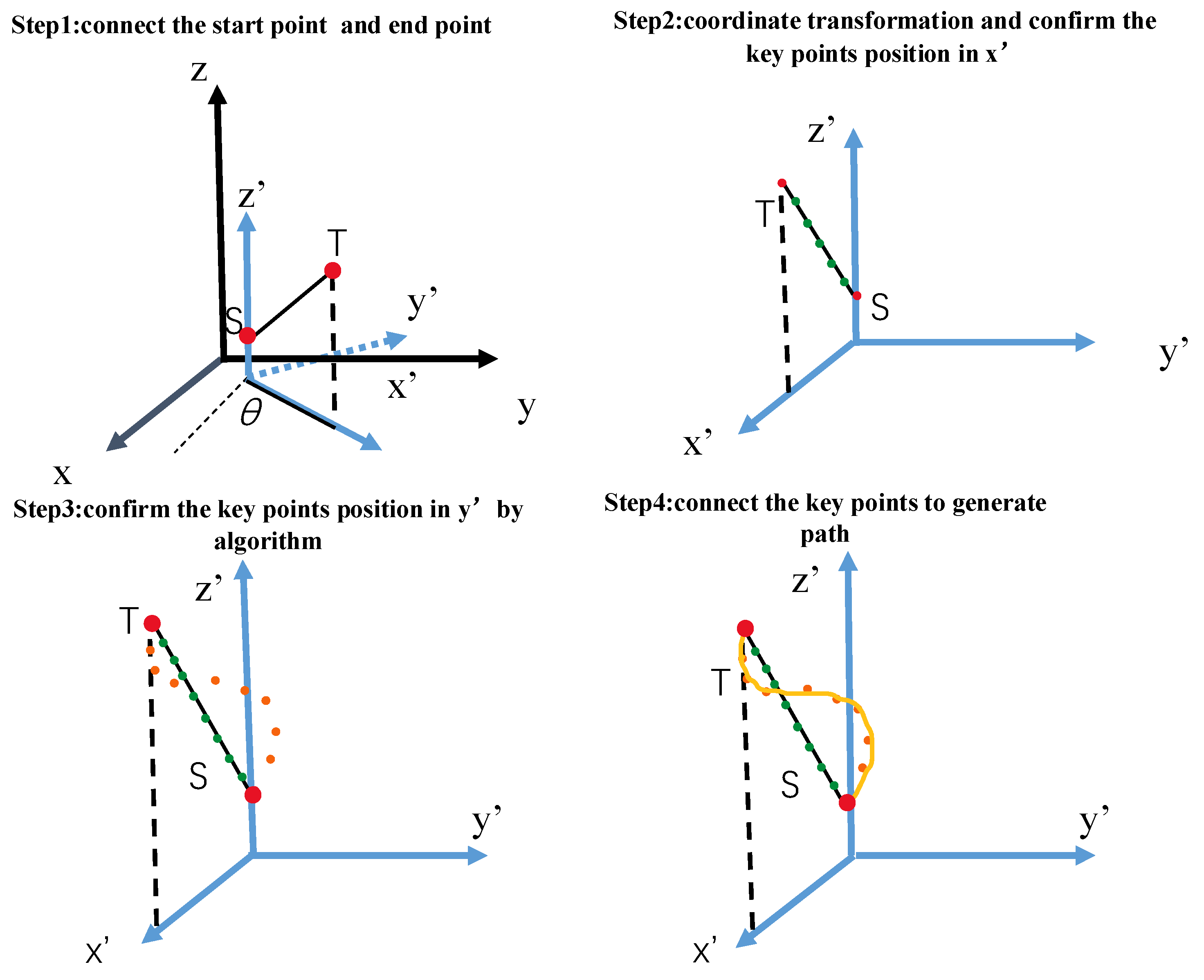
To address the path planning problem, a Cartesian coordinate system can be established and in determining the starting point (S) and the target point (T) of the UAVs in the space, the path of the UAV flight is determined by a specific number of key points in the space [44]. Define ST as the line connecting S point and T point. To reduce computational complexity and the number of decision variables for the algorithm, coordinate transformation is applied to this space. Assuming n key points are uniformly distributed along ST, segmenting ST into n + 1 intervals, and the x’-axis is fixed to the projection of the Oxy-plane of the ST through the coordinate transformation, the key points are considered to be uniformly distributed in the transformed x’-axis in x component, then the coordinates of the key points in the direction of the x’-axis can be determined by the starting and target points as well as by the number of key points. After this transformation, the optimization algorithm only needs to locate the y’ and z’ components of n key points within the constraints to determine the key points’ positions. Connecting all key points generates a path; this procedure is shown in Figure 1. The path planning problem in 2D space can be regarded as the result of projection of 3D space to the Oxy plane.
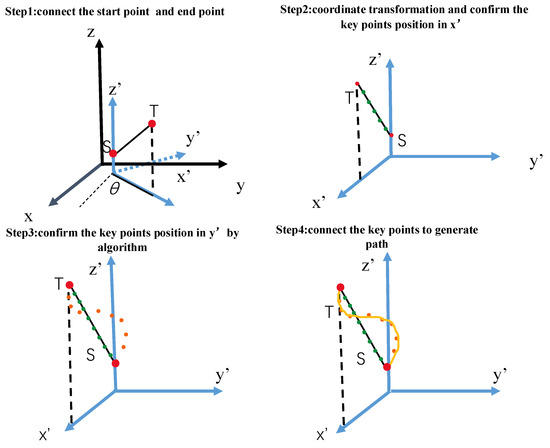
Figure 1.
Schematic diagram of the path generation principle.
The purpose of coordinate transformation is to align ST with the plane, placing S on the z’-axis, which significantly reduces computational complexity. The transformation process is described mathematically as follows:
where represents the rotation angle in the rotation matrix, denotes the coordinates in the original space and represents the coordinates in the transformed space; is the distance of S and T. For path planning on a two-dimensional plane, the above model is projected onto the plane, followed by the same steps for path planning in three-dimensional space.
2.2. Cost Function
To guide the algorithm in selecting the optimal path, we have devised a cost function to quantitatively assess the quality of the current path. The quality of the paths discovered by the algorithm can be evaluated by the cost function, and the path with lower cost will be chosen by the algorithm. To comprehensively evaluate path quality, we consider four aspects of path cost. Firstly, we need to measure the threat posed to the flight path (), which quantifies the impact of threat areas on UAV flight. This component of cost incentivizes the algorithm to generate paths that avoid threat areas as much as possible. Secondly, flight distance () is also a crucial consideration, as it strongly correlates with UAV fuel consumption. Shorter distances imply lower fuel consumption, which is not only environmentally desirable but also improves UAV efficiency. Additionally, sharp corners increase fuel consumption and diminish UAV endurance. Thus, generated paths should aim for smoothness (), quantified by the cost of corners in the flight path. Lastly, the influence of wind () on UAV flight cannot be overlooked in maritime environment. Aligning UAV flights with the direction of the wind reduces damage and fuel consumption while enhancing endurance. The overall cost function is a linear combination of these four cost components, represented mathematically as follows:
where , , and represent the weights assigned to each factor in the composite cost, and , , and are the respective cost functions for threat, distance, smoothness and wind.
2.2.1. Threat Cost
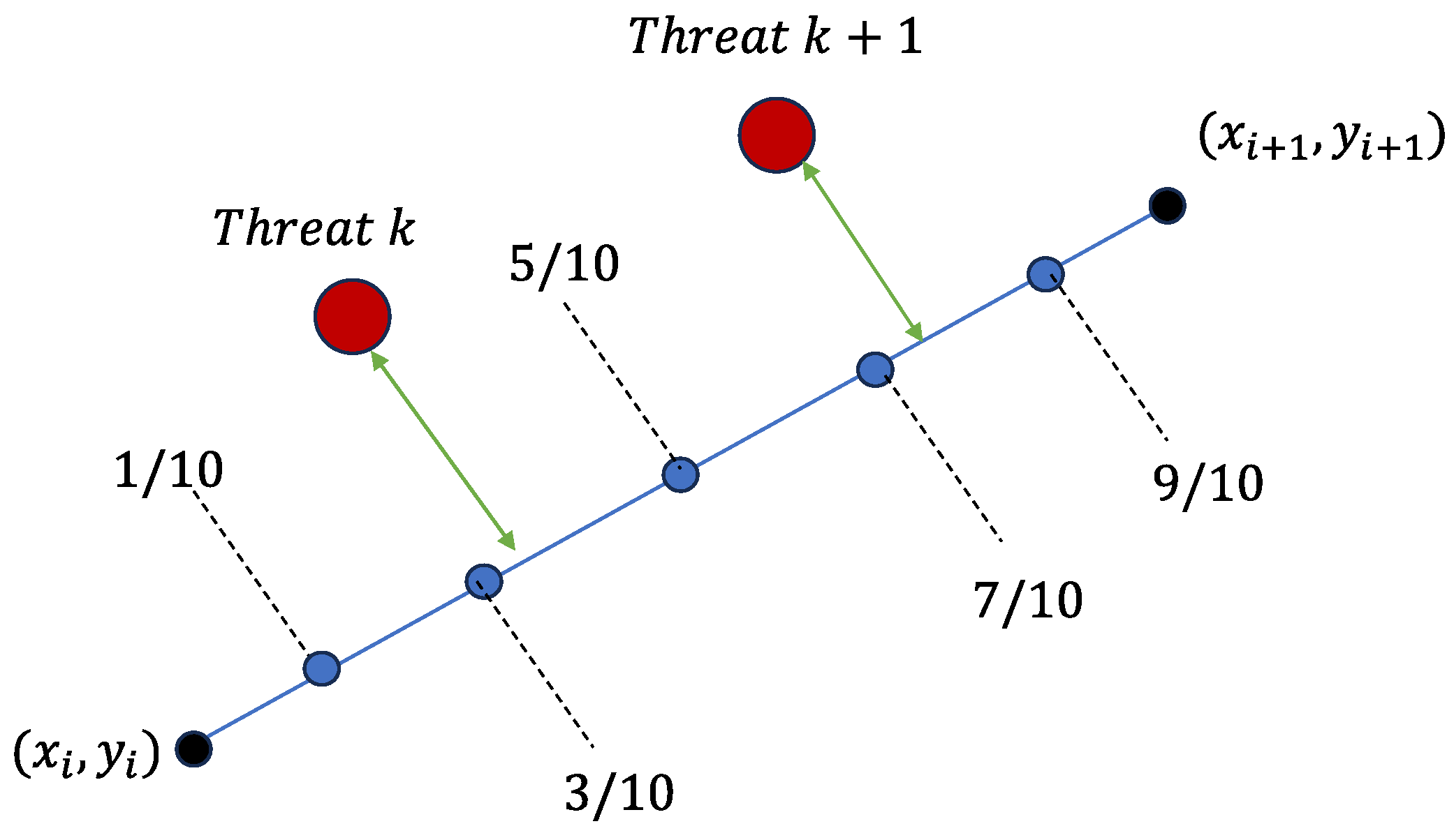
The threat cost function () evaluates the threat posed to the UAV during its flight, which is based on the distance between five particular points in each segment and the center of the threat area. It is only calculated when the UAV enters a threat area; otherwise, it remains zero. When one of the segments enters the threat area, it is not enough to evaluate the threat level by only one point, and based on the former study [44], a more accurate threat level can be obtained by selecting five points for each segment of the path that enters the threat area to assess the threat level. The severity of threat () in each threat area is determined according to the threat area. The threat cost function is formulated as follows:
where represents the length of each segment, denotes the distance between five particular points in the segment and the center of the threat area, is used to denote the severity of the kth threat area, while represents the total number of threat areas. Considering Figure 2, the crucial model in calculating the threat level is a segment of the path determined by the current key point to the preceding one, denoted as . A segment will be taken account only if this segment falls into the threat area. The total threat cost function is obtained by adding the threat degree of each segment, as shown in Equation (4).

Figure 2.
Threat level calculation schematic.
2.2.2. Path Distance
The distance function represents the cost of UAV flight, computed by summing the Euclidean distances between adjacent key points in the flight path, as described below:
where (,,) represents the spatial coordinates of the current key point, and (,,) represents the spatial coordinates of the previous key point. After obtaining the length of each segment, they are summed to obtain the total distance cost.
2.2.3. Path Smooth Cost
The smoothness cost function evaluates the smoothness of the flight path, considering both the turning angle and climbing angle. It is modeled as Equation (7).
- (1)
- Turning angle
Vigorous cornering can lead to increased fuel consumption, so the turning angle of each segment does not exceed the maximum angle . denotes the direction vector projected on the Oxy plane of the jth path segment from the jth key point to the j + 1th key point and denotes the direction vector projected on the Oxy plane from the j + 1th key point to the j + 2-th key point of the jth segment.
- (2)
- Climbing angle
The climbing angle is subject to a threshold , ensuring the UAV’s turning angle does not exceed this threshold during flight to avoid excessive fuel consumption. The climbing angle is obtained from the third-dimensional coordinates and is represented by and in Equation (9). denotes the direction vector of the j-th path segment from the j-th key point to the j + 1th key point.
2.2.4. Wind Cost
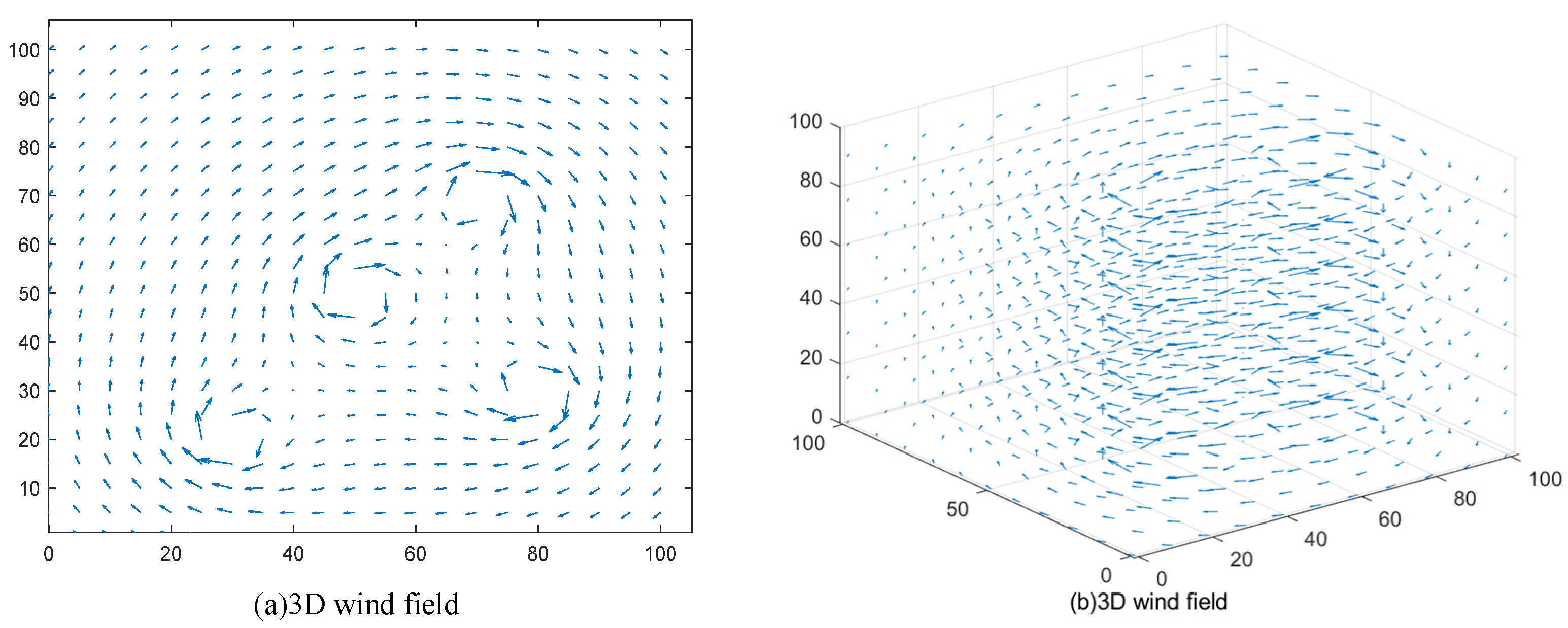
The wind cost function assesses the impact of wind on the UAV’s flight path, leveraging recorded wind intensity data. Inspired by the application of Lamb-based gas dynamics [45], this study utilizes the Lamb–Oseen vortex model to simulate vortex gas flow scenarios in an ocean scenario. The math formulation of Lamb–Oseen vortex is modeled as Equation (10). Figure 3 shows the wind environment, and includes the two-dimensional and three-dimensional wind field.
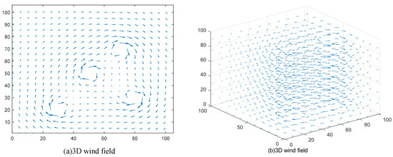
Figure 3.
The schematic representation of the wind environment.
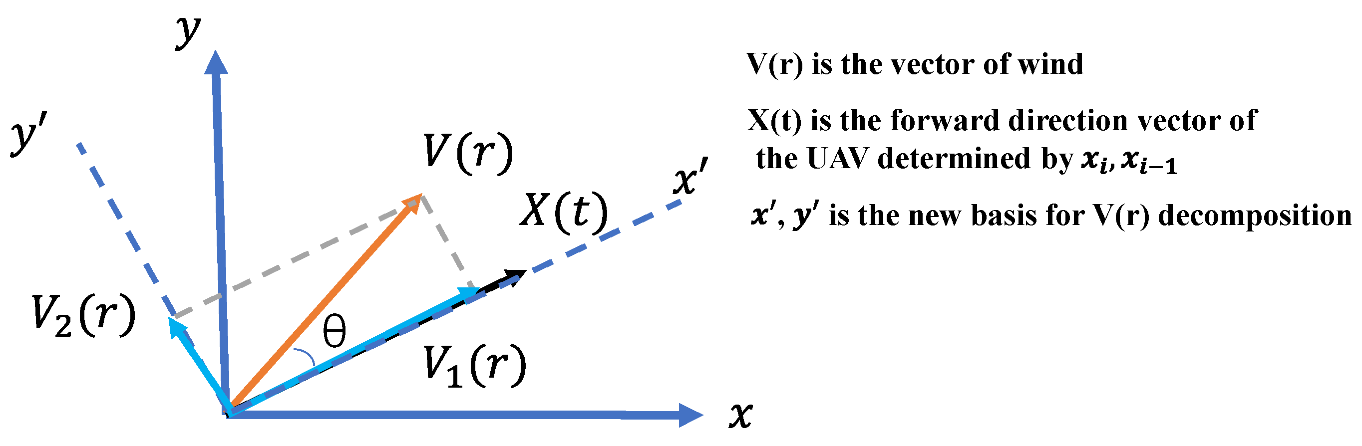
We perform slicing operations on the wind along the z-axis and calculate the cost of wind in each slicing plane. The calculation method [46] is illustrated in Figure 4, where represents the projection of the path direction vector on the plane and represents the vector of wind. By measuring the angle between and , we can project the wind vector onto the path direction and calculate the vertical and horizontal components of the wind using Equation (12). The formula projects the vector intensity at a point in the forward direction, specifically as . When is less than 90, the result is negative, indicating a downwind direction, and if not, indicating against the breeze. Additionally, the formula accounts for the direction perpendicular to the forward direction, which is represented as . This direction aims to evaluate the energy consumption bias caused by the wind, which requires energy-consuming corrections. To reduce computational complexity, we conduct calculations at five uniformly distributed locations between adjacent key points. The values obtained at all sampling points along the total path are aggregated as the result. However, as negative values may arise from this process, we normalize the results using Equation (13) to map the result to an appropriate range, thereby yielding the final cost function. In Equation (13), is a parameter that regulates the range of the interval, is a parameter representing the slope of this function. For the two-dimensional case, the same operations are performed on the plane to obtain two dimensional .

Figure 4.
The schematic diagram of wind speed cost function.
3. White Shark Optimizer
The white shark optimizer (WSO) [35], inspired by the predatory behavior of sharks in nature, is a swarm intelligence optimization algorithm invented by Malik Braiket et al. The optimization algorithm can be divided into two main stages. The first phase involves approaching the optimal prey, where each white shark autonomously seeks out potential prey within the search space or further explores promising prey locations based on detected signals. The second phase entails approaching the optimal white shark, resembling schooling behavior.
3.1. Initialization of WSO
WSO is a population-based optimization algorithm, where each shark corresponds to a solution, and the number of sharks in the population equals the number of candidate solutions. The position of a shark in the search space represents a set of decision-variable values that solve the optimization problem. The population of WSO is initialized by randomly generating a set of solutions in the solution space. All solutions of the algorithm can be represented by an , where represents the number of sharks in the population, represents the dimensionality, i.e., the number of decision variables in a solution, and the data structure is represented as follows:
Each decision variable is initialized by the following equation.
where represents the decision variable value of the jth dimension in the ith solution, represents the upper bound of the jth decision variable, represents the lower bound of the jth decision variable and is a random number uniformly distributed in the range [0, 1].
3.2. Movement Speed towards Prey
The speed at which white sharks move towards prey is updated based on the globally optimal prey position detected by the white shark population and the locally optimal prey position detected by a randomly selected white shark in the population. The abstraction of the velocity of the white shark swimming towards its prey is shown in Equation (16).
where and are random numbers in the interval [0,1]. denotes the current velocity and is defined as shown in Equation (18). is the globally optimal position obtained at the kth iteration. denotes the optimal prey position randomly selected, determined by the Equation (17).
can control the probing step size, and adjusting in can control its ability to escape from local optima. According to relevant studies, is set to 4.125 [35].
3.3. Movement towards Optimal Prey
White sharks can freely explore the search space or approach optimal prey locations based on known information. This process is mathematically modeled as follows:
where represents the position vector of the ith shark in the kth iteration and and are the upper and lower boundary vectors of the decision variables, respectively. While is the logical operator defined by Equation (26), means the different or, and stands for the bitwise not operation. The role of the logical values is defined by Equations (24)–(26). The effect of in Equation (21) is to reset the data when the range of the decision variable occurs out-of-bounds.
In swimming to the optimal prey, the frequency of undulating motion is determined by Equation (23). and represent the bound of undulation frequency of shark movement. In the context of this paper, and are 0.07 and 0.75 [35], respectively. is the main parameter used to balance exploitation and exploration behaviors.
3.4. Movement towards the Best White Shark
During the hunting process, white sharks cloud swim towards or beyond the optimal white shark. The process is mathematically modeled as follows:
represents the relative position of the i-th shark when tracking the optimal shark. , and represent random numbers in the range [0,1]. The controls the direction of shark movement, taking values of −1 or 1, indicating whether the current shark explores between the optimal shark or leaps over it. The exploration range does not exceed twice the distance between two sharks. Then, represents the distance from the i-th shark to the optimal shark, where rand denotes a random number on [0,1].
The strength of the auditory perception of white sharks determines the ability of sharks to follow the best shark. If they cannot track the best shark, they will remain where they are. refers to the strength of senses and it decides if the shark will follow the best shark. is defined by Equation (29), where balances the exploitation and exploration behaviors when executing the fish school strategy and is usually set as a constant 0.0005 [35].
3.5. Fish School Behavior
The next-generation shark position is obtained through the relative position when tracking the optimal shark and the position of the i-th shark. It synthesizes the relationship between the optimal shark and the current shark to gather at the position most likely to discover high-quality prey. This process can be mathematically described as follows:
where rand is a random number on the interval [0, 1], and represent the near optimal position and position of i-th shark, respectively.
Equation (30) indicates that sharks can adjust their position based on the position of the optimal shark closest to the prey. Eventually, the shark will be located in a position close to the optimal prey. Fish school behavior is defined based on the collective action of sharks during hunting, which can provide more possibilities for detecting optimal solutions.
4. Proposed DD-RQIWSO Algorithm for Path Planning
Due to the complexity of route planning problems in maritime transportation, three novel strategies are incorporated into the original WSO to form the proposed DD-RQIWSO algorithm, which belongs to the category of swarm intelligence algorithms. This paper employs the proposed DD-RQIWSO algorithm to solve the shortest path problem in maritime emergency transportation. Section 4.1, Section 4.2 and Section 4.3 introduce the three strategies, respectively. Section 4.4 presents the overall framework of the DD-RQIWSO algorithm for solving route planning problems. Section 4.5 analyzes the main parameters of the algorithm and Section 4.6 provides an analysis of the time complexity of DD-RQIWSO.
4.1. Directional Update Strategy
Degradation refers to the phenomenon where, during velocity update, the locally optimal value obtained by randomly selecting population individuals causes poorer individuals to fail to interact with superior individuals, resulting in stagnation and reduced exploration efficiency. To address this issue, a human learning mechanism is introduced. This mechanism is inspired by the behavior of mutual learning in human society, where individuals with weaker learning abilities tend to seek advice from superior individuals to obtain a better understanding, thereby enhancing the overall learning ability of the population. In this learning behavior, individuals with weaker learning abilities not only learn from the best individuals but also learn from inferior individuals [47].
Based on this concept, within the white shark swarm, there is a phenomenon of mutual learning. They can learn from their peers who hold advantageous positions and adjust their forward velocity by observing the exceptional individuals. Referring to the conclusion of article [47], we can categorize individuals into elite and inferior groups based on a specific population ratio and set = 5%. In simple terms, if the population size is 100, the first 5 and the last 5 particles will be chosen as the elite particle group and the underperforming particle group, respectively. The screening process is as follows: Firstly, all individuals are ranked according to their performance. Then the top of white shark individuals will be selected for the elite white shark group, and the bottom three white shark individuals will be assigned to the underperforming individuals. The specific updating strategy for the velocity involves updating the speed of the underperforming individuals randomly towards the mean value of the three white shark individuals’ positions in the elite group with the best performance. The velocity updating formula is as follows:
where and are random numbers in the interval [0,1], and are the parameters generated by Equations (19) and (20), denotes the global optimum of the kth generation and is the average of three randomly selected white sharks in the top 5% optimal white sharks, and if there are fewer than three white sharks in the top ε of the population, the average of the top three white sharks will be selected as .
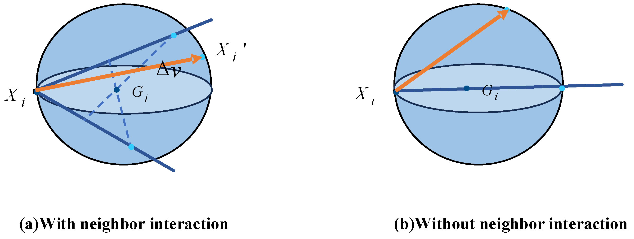
4.2. Rotational Invariant Strategy
In the fish school strategy, if the shark cannot follow the best shark, it will stay in its position. This was made into a tracking pause. This behavior will waste the chance of exploitation. In fish schooling, there is information of prey that can be used, which is acquired by itself or neighbor sharks. And this information can be applied to the rotational invariant method [48] to improve the exploitation of white sharks. The strategy of rotation invariance is based on the hyperspheres in the search space, the crucial step of this strategy is calculating the center of the hypersphere. And we modify the original strategy to increase the probability of search. The principle of modified strategy to calculate the hypersphere is shown in Figure 5.

Figure 5.
Rotational invariant strategy.
The center of the hypersphere is determined by three vectors, including , and the current shark position . Different from the original rotational invariant strategy, we use to replace the global optimal position. is the mean of the best prey location recorded by neighbor sharks, determined by Equation (32), is the shark record of the best prey location it meets. is determined by Equation (33), where denotes a fixed value of 0.1, and denotes a random number of [0,1]. It implies a random distance in the certain direction determined by current and optimal position recorded by each shark; is determined by Equation (34), where denotes a number with a fixed value of 0.1, and denotes a random number at [0, 1]. It implies a random distance in a certain direction determined by current and global optimal position. Unlike , they obtain a possibility via , which is determined by Equation (35), to remain in the current position. is a random number on the interval [0, 1]. The center coordinates of the hypersphere can be determined by Equation (36). The radius of the hypersphere is determined by the norm of the vector determined by the hypersphere center coordinates and the current shark coordinates. The velocity vector is acquired according to Equation (36). The in Equation (37) denotes the random acquisition of a point on the hypersphere. Once we obtain the velocity vector of the ith value shark, the position of the ith white shark can be updated according to the second branch of Equation (21).
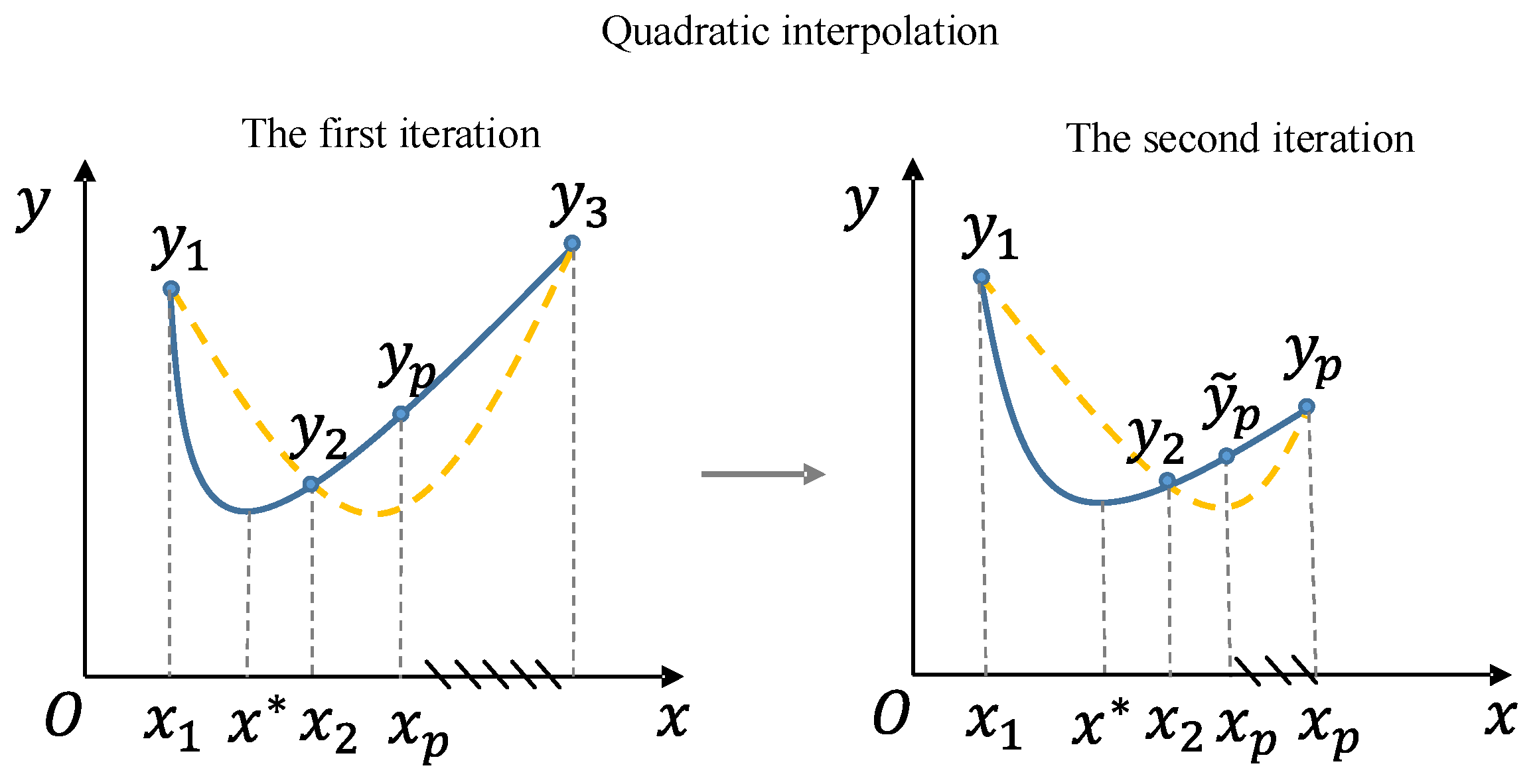
4.3. Quadratic Interpolation (QI) Operator
After the exploration and exploitation by WSO, the population can be further optimized, and quadratic interpolation (QI) modules are added. The QI operator is a method that enhances the ability of individuals to interact, further exploiting the population’s ability to mine local information. Based on the information of neighboring individuals, interpolation points are generated to deepen the exploration of known local information. When conducting quadratic interpolation on excellent individuals, it can more comprehensively explore the positions near excellent individuals, thereby searching for potentially better positions. When conducting quadratic interpolation on inferior individuals, it can drive them closer to excellent individuals and explore more valuable search ranges. The mathematical core of quadratic interpolation is to construct a parabolic fit of the objective function based on three known points, and approximate the extreme points of the objective function through the extreme points of the parabola, thereby quickly finding possible optimal values [49]. Figure 6 shows the core idea of the QI operator.
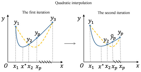
Figure 6.
Schematic diagram of quadratic interpolation.
The specific details are given as follows. denotes the population after the WSO algorithm updating. The agent in are sorted according to the cost function from lowest to highest, and we credited the sorted population as . In the population, the search agents are selected in order , and where i is increasing from 1 to n−2. The quadratic interpolation of the selected agent generation is obtained according to Equation (38), when i = n−1, n, , , and , , are chosen to obtain and , respectively. Replace with if the cost value of is superior to ’s. The equation used is as follow:
where , and respect the cost function values of three agents. After executing QI operator, the population will be formed.
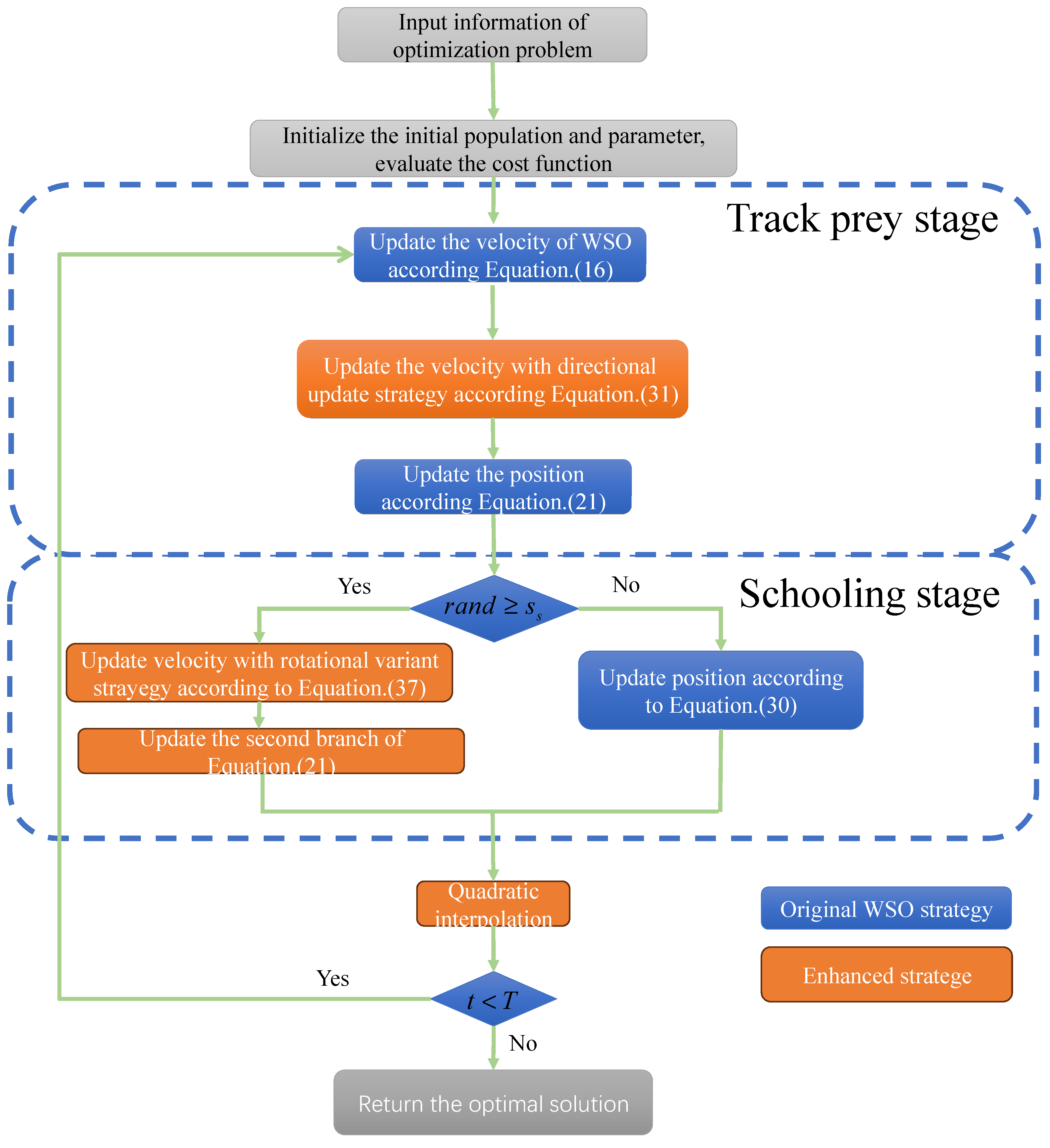
4.4. Overall Framework for Path Planning Based on DD-RQIWSO
In the DD-RQIWSO algorithm, the position of an individual represents a path from the starting point to the destination, where the number of key points in the path is considered as the dimension of the path planning problem. During the solving process of DD-RQIWSO, the position information of each white shark individual represents the coordinate components of the key points, and the dimension of the white shark individual is a variable related to the dimension of the path planning problem. In the case of a three-dimensional path planning problem, the dimension of the shark individual, denoted by , is twice the number of key points. In the position of the individual, 1 to and to represent the y-axis and z-axis coordinates of the key points in the route-planning problem, respectively; in the two-dimensional path-planning problem, the dimension of the shark individual is the same as the number of key points, representing the y-axis coordinates in the path; the x-axis coordinates are determined by the starting point, target point and the number of key points, which is illustrated in Section 2.1. A cost function is utilized to evaluate the quality of paths, guiding the algorithm in searching for the optimal solution. By searching for the position of prey in the search space, the algorithm aims to find the optimal solution, which is the shortest path. The process of DD-RQIWSO is shown in Figure 7.
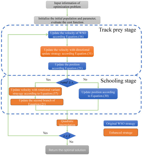
Figure 7.
The flow chart of proposed DD-RQIWSO algorithm for path planning.
The process of finding the optimal path using the DD-RQIWSO algorithm is as follows:
Step 1: Obtain information about the path planning problem, such as the number of populations and the dimension of population, initialize the parameters of DD-RQIWSO and preliminarily evaluate the paths found according to the cost function.
Step 2: Start Iteration. Update the velocity matrix according to the velocity update strategy in the WSO algorithm, and directionally update the velocity for individuals with poor performance. Update the individual positions (paths) based on this velocity matrix and the current position.
Step 3: Execute the original fish swarm algorithm or modified rotation-invariant strategy to update positions, i.e., paths for UAVs, based on the tracking ability of the white shark individuals. Evaluate the found paths and determine the detected optimal path for this iteration.
Step 4: Record the best value of cost function and the solution for path planning. Perform quadratic interpolation to interactively exchange information on detected paths, aiming to dig out potential information, which is used for the next iteration. If the iteration is equal to the max iteration, end the algorithm and return the best value and solution, or repeat from Step 2.
4.5. Parameters Analysis of DD-RQIWSO
The major parameters and their impacts are listed as follows:
and determine the frequency of the shark’s motion, which controls update step of position.
controls the effect of velocity on the position of sharks so that it can regulate the exploitation of the sharks. The value relies on τ, and fine-tuning τ decreases the probability of being trapped in local optima.
balances global exploration and local exploitation. Weather explore or exploit during an iteration relies on the value of . Its value is determined by , . The relationship between the two types of behaviors and the parameters is as follows: the exploration capability will be greater and the exploitation will be lower as the increases. Similarly, the exploration capacity will increase and the exploration capacity will decrease as the declines.
and are determined by and , which related to the iterations. They affect the velocity of the white sharks and cause the search step size to decrease with the number of iterations. Additionally, they regulate the impact of the optimal position of the white shark population on their current whereabouts.
determines the number of white sharks that need to undergo learning in the directional update strategy.
depends on and iteration. denotes the ability of following the best shark, which determines the strategy to exploitation in the fish schooling. With the iteration increased, it will tend to search around global optimal solutions rather than the optimal of individuals.
4.6. Time Complexity Analysis
For the time complexity problem of DD-RQIWSO, it is evaluated from the following aspects, including the number of sharks (n), the dimensionality of the given problem’s solution vector (d), the number of iterations (K) and the scale of the cost function (c). The specific formula for calculating the time complexity is as follows:
The components of the time complexity of Equation (40) are as follows:
1. It takes time to initialize the algorithm parameters for solving the problem.
2. It takes time to create the population and initialize its selection.
3. It takes time to the evaluate the cost function.
4. It requires time for the update of the population.
In summary, the total time complexity of DD-RQIWSO can be expressed as:
Since , , and , Equation (41) reduces to Equation (42).
This indicates that the proposed algorithm’s time complexity is polynomial. Thus, the algorithm can be considered as a time-efficient optimization algorithm. From Equation (42), it can be seen that the algorithm’s time complexity is mainly influenced by the dimension of the solution vector, the evaluation of the cost function, the number of search agents and the number of iterations, all of which depend on the nature of the problem being addressed.
5. Experiment and Results
To comprehensively evaluate the performance of the DD-RQIWSO algorithm, a series of experiments were designed for validation. Under the same environment, the proposed algorithm was compared with four advanced algorithms, including spider wasp optimizer (SWO) [50], reptile search algorithm (RSA) [33], autonomous groups particles swarm optimization (AGPSO) [51] and white shark optimizer (WSO) [35]. SWO and RSA are newly proposed swarm intelligence algorithms, and their results represent the optimization capability of the latest algorithms in this field. WSO is the original algorithm of the proposed algorithm in this paper; its results can be compared with the improved algorithm to determine the effectiveness of the improved strategy. Algorithm results based only on the original algorithm cannot show the results of the improved algorithm well, so the results of the improved algorithm by adding classical algorithms facilitate comparison with the improved algorithm proposed in this paper. The comparison algorithm is optimized in the same way as the DD-RQIWSO algorithm, as shown in Section 4.4.
All simulation experiments were conducted on a personal computer equipped with an AMD Ryzen 7 6800 H with Radeon Graphics, a 3.20 GHz processor and 16 GB of RAM, source from Lenovo (Beijing, China) and the experiments were constructed in MATLAB R2021b (9.11.0.1769968).
5.1. Experimental Setup
Experiments were conducted using a personal computer. To eliminate interference from random errors in the experimental results, each algorithm was run independently 10 times. The results showed excellent performance for each algorithm when the population size was set to 150 in the environment described in this study.
The main parameters of each algorithm are shown in Table 1. Table 2 describes the information about the threat area, while Table 3 provides information about the wind field in two and three dimensions, respectively. The z in the three-dimensional case means that the wind field is uniformly distributed along the z-axis. And this experiment only receives the horizontal wind. Additionally, the result of path denotes the best value of the algorithm in 10 independent runs. The , , and in cost function is set to 0.4, 0.3, 0.1 and 0.2, respectively. And , in Equation (13) is set to 600 and 400 according to experiment results.

Table 1.
The parameters of algorithms used for experiment.
Table 2.
The information of threat area.
Table 3.
The information of wind.
5.2. Experimental Result
5.2.1. Two-Dimensional Scenario for UAV Path Planning
- (1)
- Analysis of the experimental results of Case 1
In Case 1, seven threat areas were set up to test algorithm performance. Table 4 shows the statistical features of the results from 10 independent runs of each algorithm, including the best, worst, average and variance values. As shown in Table 4, the variance of DD-RQIWSO is 1–2 orders of magnitude smaller than the other algorithms. Although the best value of DD-RQIWSO is not superior to the best value of AGPSO in the 15 dimension, its other statistical results, including mean, worst and variance, is superior to AGPSO and other algorithms.
Table 4.
Experimental results of the value of the cost function of all algorithms for Case 1.
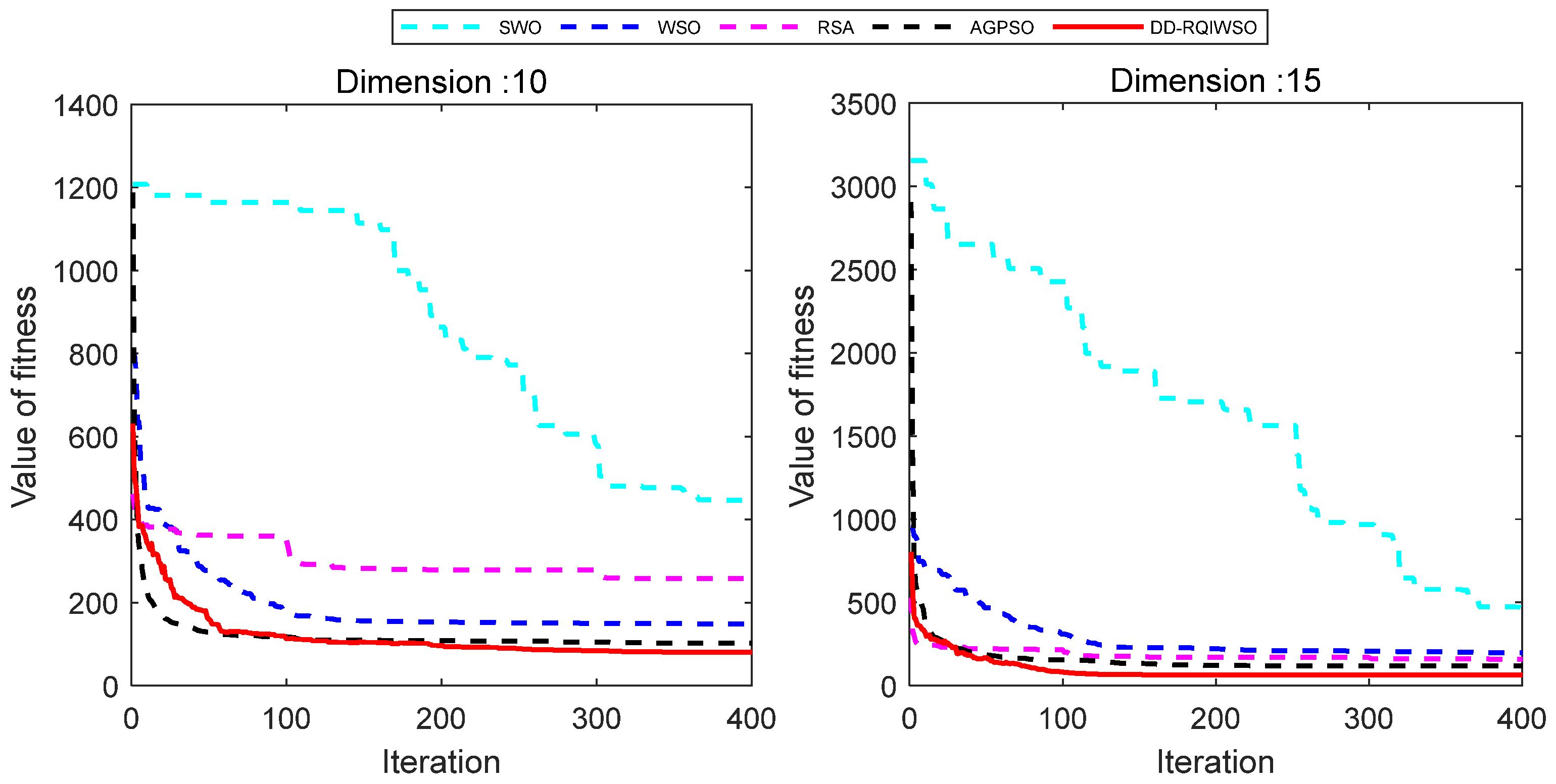
The average convergence characteristic curves of the algorithms are shown in Figure 8. According to the convergence curves, DD-RQIWSO exhibits superior convergence characteristics compared to the other four algorithms. The WSO has inferior convergence characteristics, which obtain slower optimization accuracy and fall into local optima prematurely. The accuracy of AGPSO in 10 dimension is slightly faster than the proposed algorithm, but it falls into the local optima in the end. The optimization accuracy of SWO is slow and the final value of cost function is the worst among all algorithm we test.
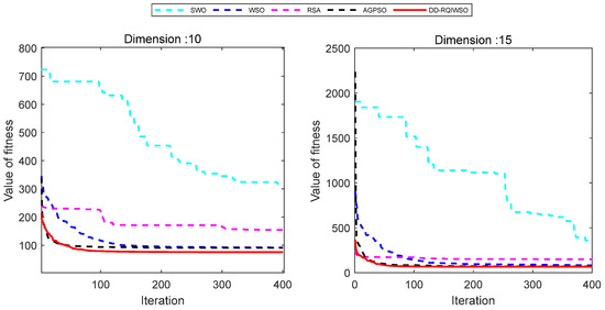
Figure 8.
The mean accuracy convergence curves for Case 1.
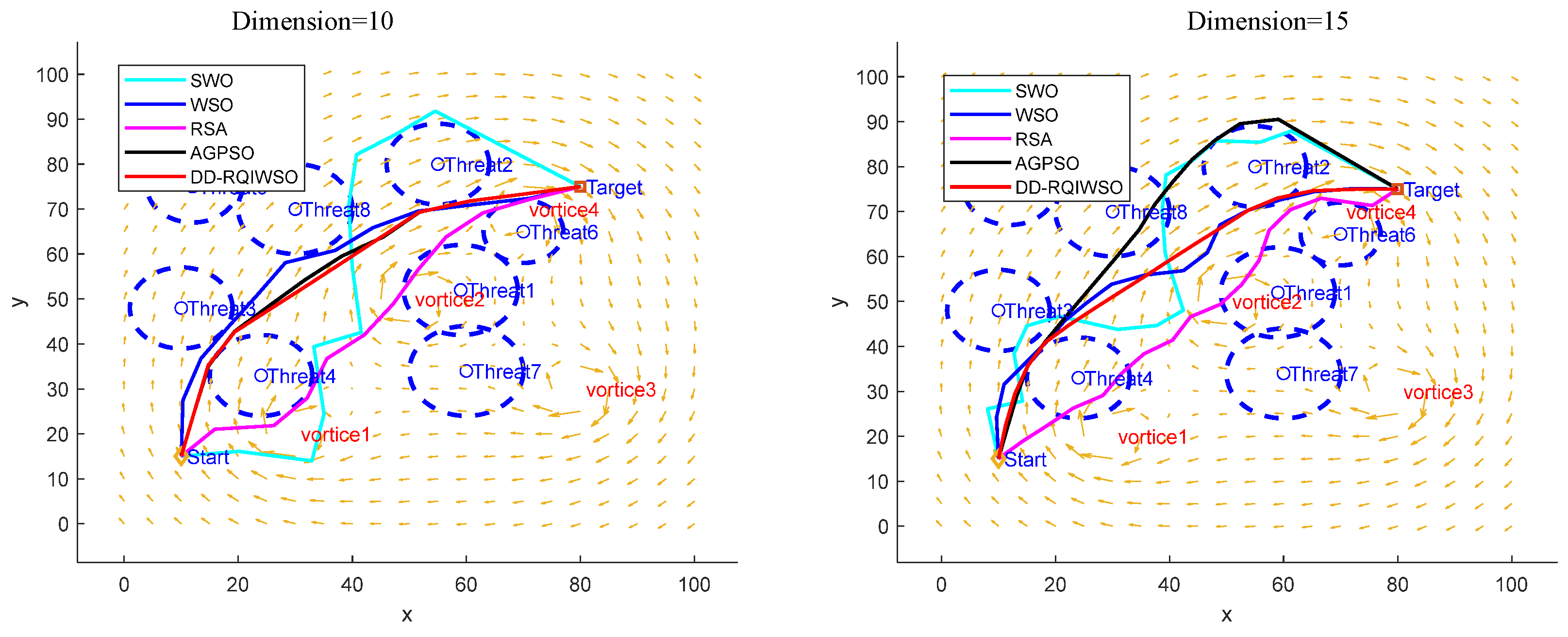
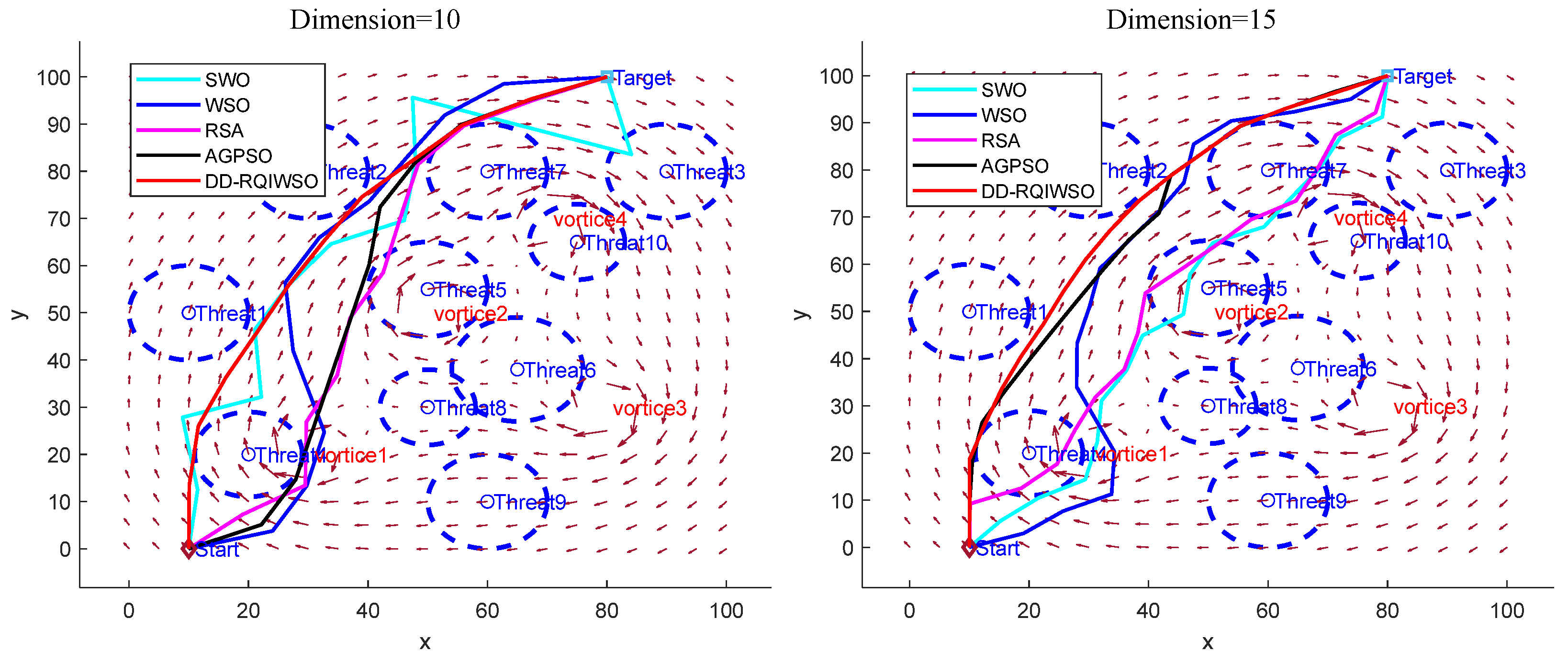
Figure 9 shows the 2D flight path results of each algorithm. Compared with the original WSO algorithm, this path of DD-RQIWSO is shorter, smoother and bypassing the threat regions. The AGPSO, also known as the improved algorithm, does not perform as well as DD-RQIWSO. In the 10 dimension, the paths of AGPSO and DD-RQIWSO are similar, but in the 15 dimension, AGPSO takes the farther path, and passes through the threat regions. RSA does not possess the ability to plan paths that consider the environment. SWO takes a rough route and long distance in this case.
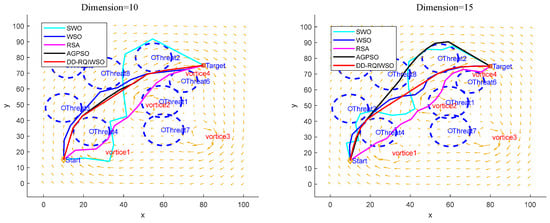
Figure 9.
Flight paths for UAV in Case 1.
- (2)
- Analysis of the experimental results of Case 2
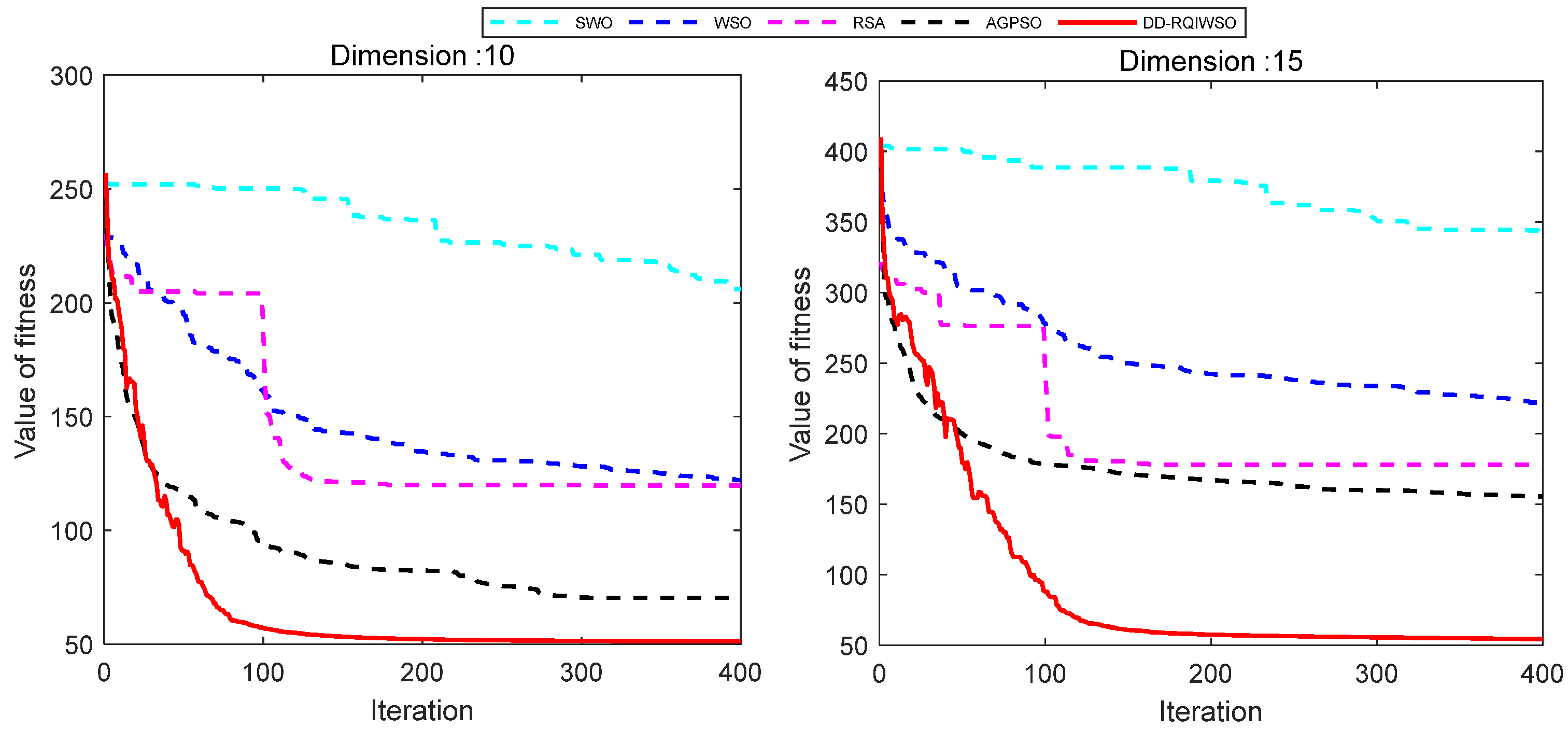
In the second case, the number of threat regions is more than Case 1. The statistical results of 10 independent runs of Case 2 are shown in Table 5. As can be observed from the table, the DD-RQIWSO algorithm provides a good quality path planning for UAVs. The optimal solutions it obtains are better than those obtained from other compared algorithms in terms of the best, worst and mean value. The average convergence curves of these algorithms are presented in Figure 10. It can be seen from the figure that DD-RQIWSO is superior to other algorithms in both final convergence results and convergence speed at 15 dimensions. The convergence accuracy of AGPSO is only slightly faster than the proposed algorithm in 10 dimension, and all of the solutions of AGPSO finally fall into local optima. The performance of SWO is the worst; the convergence accuracy is slowest among all the compared algorithms. The WSO is worse than DD-RQIWSO from convergence accuracy and final solutions in any dimensions.
Table 5.
Experimental results of the value of the cost function of all algorithms for Case 2.
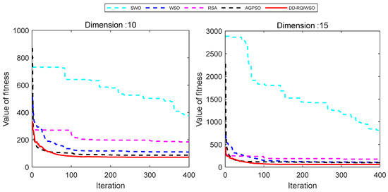
Figure 10.
The mean accuracy convergence curves for Case 2.
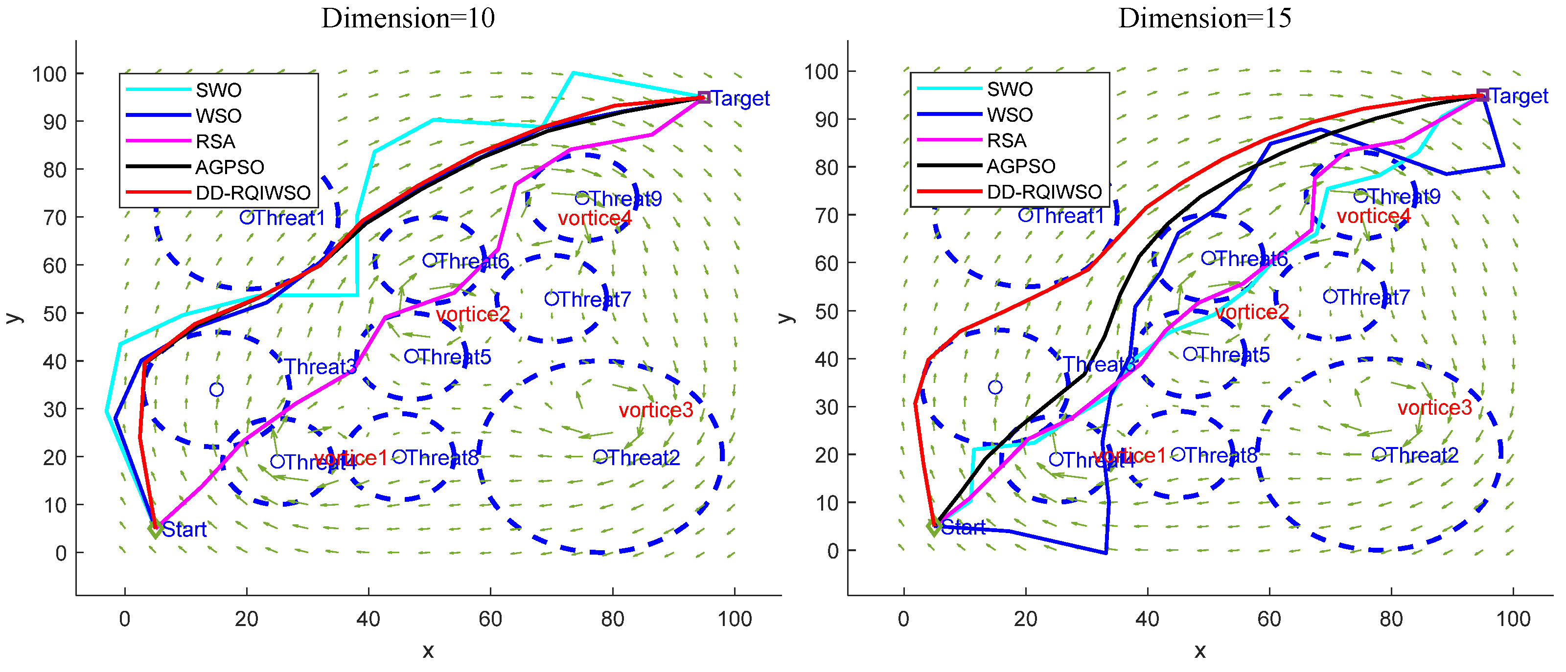
The path results are shown in Figure 11. The DD-RQIWSO algorithm obtains the optimal path with respect to the other compared algorithms. Not only does the path of DD-RQIWSO successfully bypass the threat regions, but also obtains relative minimum distance. Meanwhile, this path takes into account the effects of wind and offers fairly good path smoothness. The paths generated by the original WSO algorithm yield a poor performance in this case, which not only take further distances, but also fly against the wind. AGPSO claims similar results with DD-RQIWSO in the 15 dimension, but falls into local optima and even exists unnecessarily far from the target in the 10 dimension. SWO and RSA get low ability to detect the search space and yield bad paths.

Figure 11.
Flight paths for UAVs in Case 2.
- (3)
- Analysis of the experimental results of Case 3
The experiment results for Case 3 are shown in Table 6. These statistical outcomes show that DD-RQIWSO outperforms other compared algorithms. All of its statistical results are superior to the compared algorithms. The DD-RQIWSO obtains the optimal cost function value and has optimal stability, which is proved by these statistical results. The curves describing the features of convergence yield by algorithms are given in Figure 12. According to these convergence curves, DD-RQIWSO outperforms WSO and SWO algorithms. In some situations, RSA and AGPSO convergence outperforms DD-RQIWSO in certain aspects, as analyzed below. The RSA algorithm has good convergence accuracy in the early iterations, but its final convergence value is worse than that of the proposed algorithm and fails to escape from local optima. The convergence accuracy of AGPSO in 10 dimension is faster than DD-RQIWSO, but it does not skip out of the local optimum until the end. SWO shows the worst performance. WSO is worse than AGPSO, but they have similar convergence curves.
Table 6.
Experimental results of the value of the cost function of all algorithms for test Case 3.
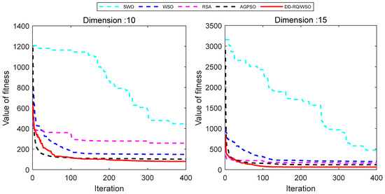
Figure 12.
The mean accuracy convergence curves for Case 3.
As shown in Figure 13, the path of DD-RQIWSO algorithm obtains the optimal path with respect to the other compared algorithms. Compared to the other algorithms, the paths of DD-RQIWSO are smoother. WSO has acceptable results in the 10-dimension case. But once the dimensions are elevated, it loses the ability to take the environment into account. The result of AGPSO is similar to DD-RQIWSO in the 10 dimension, but it takes the farther path, and passes through the threat regions more seriously than DD-RQIWSO in the 15 dimension. SWO follows a rough route and long distance in the 10 dimension, and essentially loses the ability to plan paths that consider the environment in the 15 dimension. And RSA does not possess the ability to plan paths that consider the environment in this case.
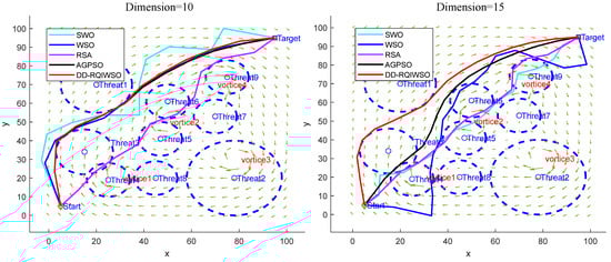
Figure 13.
Flight paths for UAVs in Case 3.
5.2.2. Three-Dimensional Scenario for UAV Path Planning
- (1)
- Analysis of the experimental results of Case 4
In the fourth test, a complex three-dimensional scenario was constructed to test the performance of the proposed algorithm and other state-of-the-art algorithms. Table 7 shows the numerical features of all algorithms’ statistical results. As we can see from the table, DD-RQIWSO presents strong stability. Its value of cost function maintains in an excellent level. The best value of AGPSO is lower than DD-RQIWSO in the 10 dimension, but its results are too scattered. In contrast, RSA presents good stability, but the value of cost function is too high compared with DD-RQIWSO. From a general point of view, the DD-RQIWSO shows stable maintenance of a better range of results.
Table 7.
Experimental results of the value of the cost function of all algorithms for test Case 4.
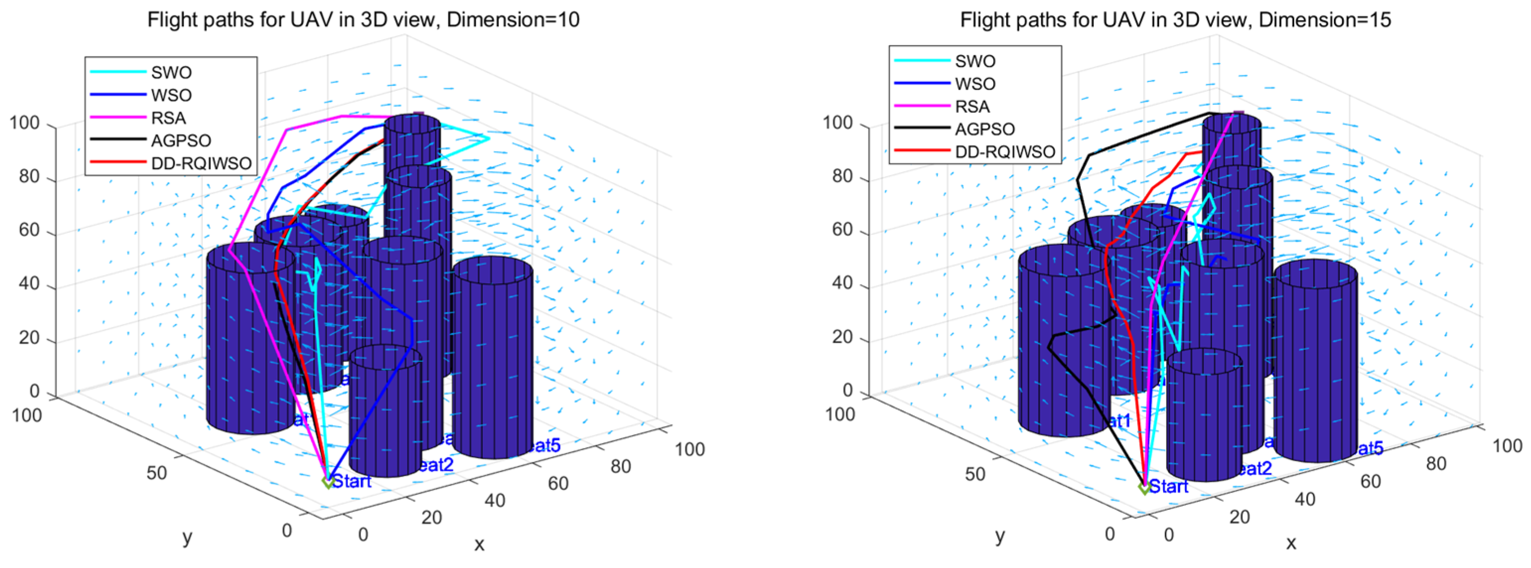
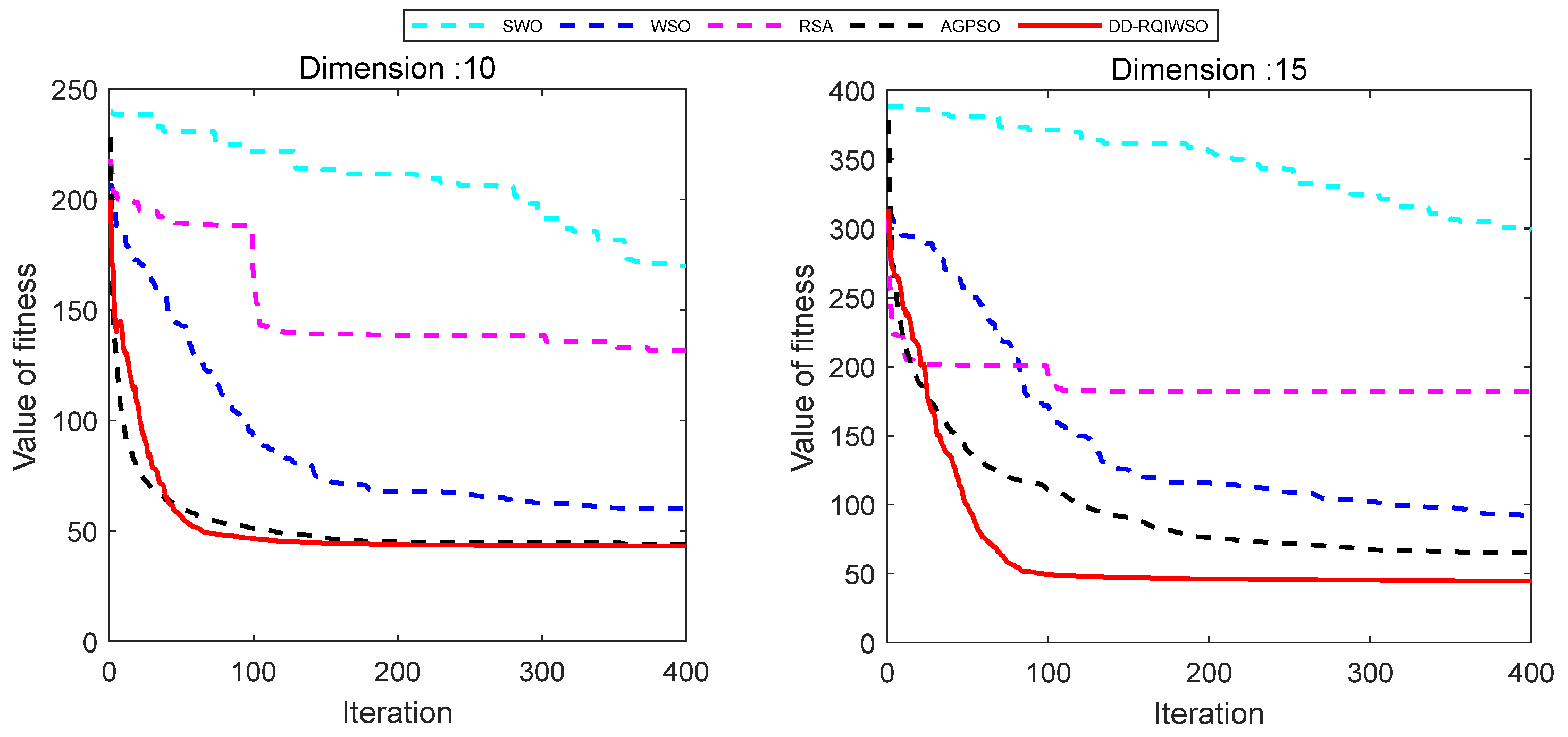
Figure 14 exhibits the convergence curves of results of the algorithms. The convergence characteristics of the DD-RQIWSO algorithm excel in comparison to the other algorithms, which can be proved by Figure 14. The convergence accuracy of AGPSO algorithm is little faster than DD-RQIWSO before 15 generations; it also slows down and falls into local optima after that. There is no doubt that the proposed algorithm obtains the optima solution at the fastest accuracy. The flight paths of the UAVs generated by each algorithm in a 3D environment are shown in Figure 15. As shown in the figure, the path of DD-RQIWSO algorithm obtains the optimal path with respect to the other compared algorithms. The flight path of DD-RQIWSO algorithm follows a smooth path. It avoids all threats as it takes advantage of wind. The path generated by WSO becomes tortuous and follows an unwarranted route. The flight path of RSA algorithm provides higher flight attitude in the 15 dimension and increases flight distance in the 10 dimension. SWO’s path twists the route and goes through the threat region usually. The path of AGPSO follows long routes when dimension increases, and loses the ability to consider the effect of the environment.
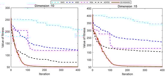
Figure 14.
The mean accuracy convergence curves for Case 4.
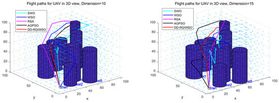
Figure 15.
Flight paths for UAVs in Case 4 in 10, 15 dimensions.
- (2)
- Analysis of the experimental results of Case 5
The environment of this case is more oriented towards the effect of wind on UAVs, excluding the effect of obstacles superimposed on the wind field. Table 8 presents the statistical features of the cost functions of each algorithm in the final experimental scenario. As shown in the table, DD-RQIWSO outperforms other algorithms in most statistical features, only the best result of AGPSO slightly lower than the proposed algorithm. This indicates that the proposed algorithm exhibits excellent optimization performance and stability in this scenario.
Table 8.
Experimental results of the value of the cost function of all algorithms for test Case 5.
Figure 16 depicts the average convergence curves generated by each algorithm. From the figure, it can be observed that the proposed algorithm has good convergence characteristics. Although the optimization accuracy of the RSA algorithm in 15 dimensions is faster at about 20 generations, it is finally overtaken by the DD-RQIWSO algorithm. As for AGPSO, it presents excellent optimization accuracy in low dimension, but not superior to DD-RQIWSO. As we can observe, SWO and WSO algorithms fall into local optima prematurely, and the accuracy of SWO is pretty bad. Figure 17 illustrates the minimum-cost UAV route generated by algorithms. As can be seen from these figures, the flight paths of DD-RQIWSO demonstrate more efficient obstacle avoidance capabilities. The flight paths of SWO even run through the threat regions in 15 dimensions, and the result of WSO is no longer smooth and through the threat region.
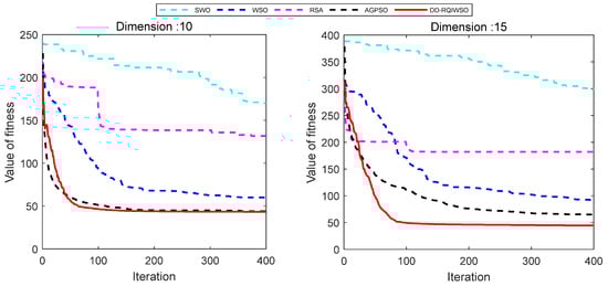
Figure 16.
The mean accuracy convergence curves for Case 5.

Figure 17.
The path planning for Case 5 in 10, 15 dimensions.
5.3. Time Analysis
When evaluating the cost of the wind direction, the cost is calculated one time for each sampling point, and the number of sampling points is only related to the number of key points of the path in the algorithm, so it can be found that the path planning can be finished in linear time no matter whether it considers the influence of the wind or not, i.e., the algorithm’s time complexity is still O(n).
The running time of if adding the wind field are shown to evaluate the actual time overhead brought by considering the wind field factor, from the results, the algorithm does not lead to the explosive growth of computing time due to the wind factor, and its computation time is acceptable. Under the condition of obtaining reliable paths, the running time required by the proposed algorithm in this paper is also in line with the range of running time of the algorithms in existing research [36]. The results are shown in Table 9 and Table 10.
Table 9.
Comparison of running time of test algorithm for Case 1 in two dimensions.
Table 10.
Comparison of running time of test algorithm for Case 4 in three dimensions.
5.4. Discussion
This study investigated the path planning problem of UAVs under emergency transportation in the marine environment. Optimization algorithms based on swarm intelligence have demonstrated excellent optimization capabilities that can deal with a variety of complex mathematical models and find the optimal solution as long as a suitable cost function is constructed. In this paper, a model of maritime emergency transportation environment is constructed, and the WSO algorithm is further improved so that it yields a good performance in path planning in maritime emergency transportation environment. As validated by experimental results, the proposed algorithm can provide suitable flight routes for UAVs, so that the UAVs can avoid obstacles with the shortest paths and utilize the wind environment as much as possible to reduce energy consumption. Although the experimental results in Section 5.2 show that DD-RQIWSO has a good performance, there are still limitations in the research. In this paper, the wind field under the mathematical model is relatively simple and cannot fully simulate the complex wind direction in nature. Also, the method proposed in this paper cannot handle real-time tasks. Proven by the experiment, as one of problems in the application of UAVs to maritime emergency transportation, the path-planning problem of UAVs can be addressed by the proposed algorithm.
6. Conclusions
Path planning with complex constraints for UAVs is a hard optimization problem. This paper proposes a new swarm intelligence algorithm to solve this problem. Based on the WSO algorithm, three strategies are incorporated so that it can work more effectively. These strategies are as follows: Firstly, a more elaborate velocity update mechanism is introduced to the algorithm. For the poorly performing individuals, we make them learn from the elites and update their speed based on the position of the elites, thus improving the exploitation ability of the algorithm. Secondly, a modified rotation invariant strategy complements the fish schooling strategy to enhance algorithmic exploitation when they lose the position of the best shark. Finally, a QI operator conducts further fine-tuning of the existing solutions detected by the algorithm at each iteration. It interacts with the information between individuals for existing feasible solutions, so that the high-performing individuals can perform more detailed exploitation, and the low-performing individuals can interact directly with the high-performing individuals to move closer to the optimum. To describe the maritime emergency transportation environment, a maritime environment model is constructed. It considers the effect of obstacles and wind. Through a series of comparative experiments, the research in this paper can effectively solve the path-planning problem of UAVs.
In addition, the study could still be explored further. Firstly, the results in this paper are only for wind fields with a single flow direction. How to utilize more complex wind fields in the 3D case, such as considering tangential wind, for effective path planning is a worthwhile research direction. Secondly, the DD-RQIWSO algorithm’s need to further reduce time consumption is required for the algorithm proposed in this study to handle real-time problems. Thirdly, it is also useful to utilize the DD-RQIWSO algorithm to address other optimization problems in UAVs, such as multi-UAVs cooperative emergency transportation path planning.
Author Contributions
Conceptualization, F.M. and H.L; methodology, F.M. and H.L.; software, F.M. and H.L.; validation, X.M., F.M. and G.Y.; formal analysis, X.M., W.Z. and T.L.; investigation, H.L., G.Y., W.Z. and T.L.; writing—original draft preparation, F.M. and H.L.; writing—review and editing, F.M., X.M. and W.Z.; visualization, F.M., H.Z. and G.Y.; supervision, X.M. and F.M.; funding acquisition, X.M. and Z.W. All authors have read and agreed to the published version of the manuscript.
Funding
This work was supported in part by the National Key Research and Development Program of China under grant No. 2021YFC2801002, the National Natural Science Foundation of China under grant No. 52201401, grant No. 52331012, grant No. 52071200; in part by; in part by the Shanghai Committee of Science and Technology, China, under grant No. 23010502000; in part by the Shanghai Science and Program of Shanghai Academic/Technology Research Leader under grant No. 22XD1431000.
Institutional Review Board Statement
Not applicable.
Informed Consent Statement
Not applicable.
Data Availability Statement
Data are contained within the article.
Acknowledgments
The authors would like to thank the anonymous reviewers for their valuable comments.
Conflicts of Interest
Author Zhongdai Wu was employed by the Shanghai Ship and Shipping Research Institute Co., Ltd., The remaining authors declare that the research was conducted in the absence of any commercial or financial relationships that could be construed as a potential conflict of interest.
References
- Mohsan, S.A.H.; Othman, N.Q.H.; Li, Y.; Alsharif, M.H.; Khan, M.A. Unmanned Aerial Vehicles (UAVs): Practical Aspects, Applications, Open Challenges, Security Issues, and Future Trends. Intell. Serv. Robot. 2023, 16, 109–137. [Google Scholar] [CrossRef]
- Menouar, H.; Guvenc, I.; Akkaya, K.; Uluagac, A.S.; Kadri, A.; Tuncer, A. UAV-Enabled Intelligent Transportation Systems for the Smart City: Applications and Challenges. IEEE Commun. Mag. 2017, 55, 22–28. [Google Scholar] [CrossRef]
- Kaamin, M.; Razali, S.N.M.; Ahmad, N.F.A.; Bukari, S.M.; Ngadiman, N.; Kadir, A.A.; Hamid, N.B. The Application of Micro UAV in Construction Project. AIP Conf. Proc. 2017, 1891, 020070. [Google Scholar] [CrossRef]
- Sivakumar, M.; Tyj, N.M. A Literature Survey of Unmanned Aerial Vehicle Usage for Civil Applications. J. Aerosp. Technol. Manag. 2021, 13, e4021. [Google Scholar] [CrossRef]
- Chen, X.; Liu, S.; Liu, R.W.; Wu, H.; Han, B.; Zhao, J. Quantifying Arctic Oil Spilling Event Risk by Integrating an Analytic Network Process and a Fuzzy Comprehensive Evaluation Model. Ocean Coast. Manag. 2022, 228, 106326. [Google Scholar] [CrossRef]
- Chen, X.; Wei, C.; Yang, Y.; Luo, L.; Biancardo, S.A.; Mei, X. Personnel Trajectory Extraction from Port-Like Videos Under Varied Rainy Interferences. IEEE Trans. Intell. Transp. Syst. 2024, 25, 6567–6579. [Google Scholar] [CrossRef]
- Ma, D.; Ma, T.; Li, Y.; Ling, Y.; Ben, Y. A Contour-Based Path Planning Method for Terrain-Aided Navigation Systems with a Single Beam Echo Sounder. Measurement 2024, 226, 114089. [Google Scholar] [CrossRef]
- Xia, J.; Ma, T.; Li, Y.; Xu, S.; Qi, H. A Scale-Aware Monocular Odometry for Fishnet Inspection with Both Repeated and Weak Features. IEEE Trans. Instrum. Meas. 2023, 73, 5001911. [Google Scholar] [CrossRef]
- Yan, R.; Wang, S.; Zhen, L.; Laporte, G. Emerging Approaches Applied to Maritime Transport Research: Past and Future. Commun. Transp. Res. 2021, 1, 100011. [Google Scholar] [CrossRef]
- Zhang, Q.; Wu, H.; Mei, X.; Han, D.; Marino, M.D.; Li, K.-C.; Guo, S. A Sparse Sensor Placement Strategy Based on Information Entropy and Data Reconstruction for Ocean Monitoring. IEEE Internet Things J. 2023, 10, 19681–19694. [Google Scholar] [CrossRef]
- Mei, X.; Han, D.; Saeed, N.; Wu, H.; Han, B.; Li, K.-C. Localization in Underwater Acoustic IoT Networks: Dealing with Perturbed Anchors and Stratification. IEEE Internet Things J. 2024, 11, 17757–17769. [Google Scholar] [CrossRef]
- Mei, X.; Han, D.; Saeed, N.; Wu, H.; Ma, T.; Xian, J. Range Difference-Based Target Localization under Stratification Effect and NLOS Bias in UWSNs. IEEE Wirel. Commun. Lett. 2022, 11, 2080–2084. [Google Scholar] [CrossRef]
- Gasparetto, A.; Boscariol, P.; Lanzutti, A.; Vidoni, R. Path Planning and Trajectory Planning Algorithms: A General Overview. In Motion and Operation Planning of Robotic Systems: Background and Practical Approaches; Carbone, G., Gomez-Bravo, F., Eds.; Springer International Publishing: Cham, Switzerland, 2015; pp. 3–27. ISBN 978-3-319-14705-5. [Google Scholar]
- Huo, L.; Zhu, J.; Li, Z.; Ma, M. A Hybrid Differential Symbiotic Organisms Search Algorithm for UAV Path Planning. Sensors 2021, 21, 3037. [Google Scholar] [CrossRef] [PubMed]
- Papadimitriou, C.H.; Steiglitz, K. Combinatorial Optimization: Algorithms and Complexity; Courier Corporation: Washington, DC, USA, 1998; ISBN 978-0-486-40258-1. [Google Scholar]
- Hart, P.E.; Nilsson, N.J.; Raphael, B. A Formal Basis for the Heuristic Determination of Minimum Cost Paths. IEEE Trans. Syst. Sci. Cybern. 1968, 4, 100–107. [Google Scholar] [CrossRef]
- Kuffner, J.J.; LaValle, S.M. RRT-Connect: An Efficient Approach to Single-Query Path Planning. In Proceedings of the 2000 ICRA. Millennium Conference, IEEE International Conference on Robotics and Automation, Symposia Proceedings (Cat. No. 00CH37065), San Francisco, CA, USA, 24–28 April 2000; Volume 2, pp. 995–1001. [Google Scholar]
- Kavraki, L.E.; Svestka, P.; Latombe, J.-C.; Overmars, M.H. Probabilistic Roadmaps for Path Planning in High-Dimensional Configuration Spaces. IEEE Trans. Robot. Autom. 1996, 12, 566–580. [Google Scholar] [CrossRef]
- Bayili, S.; Polat, F. Limited-Damage A*: A Path Search Algorithm That Considers Damage as a Feasibility Criterion. Knowl.-Based Syst. 2011, 24, 501–512. [Google Scholar] [CrossRef]
- Moon, C.; Chung, W. Kinodynamic Planner Dual-Tree RRT (DT-RRT) for Two-Wheeled Mobile Robots Using the Rapidly Exploring Random Tree. IEEE Trans. Ind. Electron. 2015, 62, 1080–1090. [Google Scholar] [CrossRef]
- El-Kenawy, E.-S.M.; Eid, M.M.; Abdelhamid, A.A.; Ibrahim, A.; Takieldeen, A.E.; Elkhalik, S.H.A. Hybrid Particle Swarm and Gray Wolf Optimization for Prediction of Appliances in Low-Energy Houses. In Proceedings of the 2022 International Telecommunications Conference (ITC-Egypt), Alexandria, Egypt, 26–28 July 2022; pp. 1–5. [Google Scholar]
- Mei, X.; Miao, F.; Wang, W.; Wu, H.; Han, B.; Wu, Z.; Chen, X.; Xian, J.; Zhang, Y.; Zang, Y. Enhanced Target Localization in the Internet of Underwater Things through Quantum-Behaved Metaheuristic Optimization with Multi-Strategy Integration. J. Mar. Sci. Eng. 2024, 12, 1024. [Google Scholar] [CrossRef]
- Abdel-Basset, M.; Mohamed, R.; AbdelAziz, N.M.; Abouhawwash, M. HWOA: A Hybrid Whale Optimization Algorithm with a Novel Local Minima Avoidance Method for Multi-Level Thresholding Color Image Segmentation. Expert Syst. Appl. 2022, 190, 116145. [Google Scholar] [CrossRef]
- Zeng, Z.; Sammut, K.; Lian, L.; He, F.; Lammas, A.; Tang, Y. A Comparison of Optimization Techniques for AUV Path Planning in Environments with Ocean Currents. Robot. Auton. Syst. 2016, 82, 61–72. [Google Scholar] [CrossRef]
- SinghPal, N.; Sharma, S. Robot Path Planning Using Swarm Intelligence: A Survey. Int. J. Comput. Appl. 2013, 83, 5–12. [Google Scholar] [CrossRef]
- Li, G.; Chou, W. Path Planning for Mobile Robot Using Self-Adaptive Learning Particle Swarm Optimization. Sci. China Inf. Sci. 2017, 61, 052204. [Google Scholar] [CrossRef]
- Zhu, H.; Wang, Y.; Li, X. UCAV Path Planning for Avoiding Obstacles Using Cooperative Co-Evolution Spider Monkey Optimization. Knowl.-Based Syst. 2022, 246, 108713. [Google Scholar] [CrossRef]
- Niu, Y.; Yan, X.; Wang, Y.; Niu, Y. Three-Dimensional UCAV Path Planning Using a Novel Modified Artificial Ecosystem Optimizer. Expert Syst. Appl. 2023, 217, 119499. [Google Scholar] [CrossRef]
- Cai, J.; Zhang, F.; Sun, S.; Li, T. A Meta-Heuristic Assisted Underwater Glider Path Planning Method. Ocean Eng. 2021, 242, 110121. [Google Scholar] [CrossRef]
- Specht, M.; Widźgowski, S.; Stateczny, A.; Specht, C.; Specht, O. Comparative Analysis of Unmanned Aerial Vehicles Used in Photogrammetric Surveys. TransNav Int. J. Mar. Navig. Saf. Od Sea Transp. 2023, 17, 433–443. [Google Scholar] [CrossRef]
- Wolpert, D.H.; Macready, W.G. No Free Lunch Theorems for Optimization. IEEE Trans. Evol. Comput. 1997, 1, 67–82. [Google Scholar] [CrossRef]
- Zervoudakis, K.; Tsafarakis, S. A Mayfly Optimization Algorithm. Comput. Ind. Eng. 2020, 145, 106559. [Google Scholar] [CrossRef]
- Abualigah, L.; Elaziz, M.A.; Sumari, P.; Geem, Z.W.; Gandomi, A.H. Reptile Search Algorithm (RSA): A Nature-Inspired Meta-Heuristic Optimizer. Expert Syst. Appl. 2022, 191, 116158. [Google Scholar] [CrossRef]
- Zhong, C.; Li, G.; Meng, Z. Beluga Whale Optimization: A Novel Nature-Inspired Metaheuristic Algorithm. Knowl.-Based Syst. 2022, 251, 109215. [Google Scholar] [CrossRef]
- Braik, M.; Hammouri, A.; Atwan, J.; Al-Betar, M.A.; Awadallah, M.A. White Shark Optimizer: A Novel Bio-Inspired Meta-Heuristic Algorithm for Global Optimization Problems. Knowl.-Based Syst. 2022, 243, 108457. [Google Scholar] [CrossRef]
- Liang, J.; Liu, L. Optimal Path Planning Method for Unmanned Surface Vehicles Based on Improved Shark-Inspired Algorithm. J. Mar. Sci. Eng. 2023, 11, 1386. [Google Scholar] [CrossRef]
- Farhat, M.; Kamel, S.; Elseify, M.A.; Abdelaziz, A.Y. A Modified White Shark Optimizer for Optimal Power Flow Considering Uncertainty of Renewable Energy Sources. Sci. Rep. 2024, 14, 3051. [Google Scholar] [CrossRef] [PubMed]
- Ali, M.A.; Kamel, S.; Hassan, M.H.; Ahmed, E.M.; Alanazi, M. Optimal Power Flow Solution of Power Systems with Renewable Energy Sources Using White Sharks Algorithm. Sustainability 2022, 14, 6049. [Google Scholar] [CrossRef]
- Mustafa, H.M.J.; Al-Zyod, M.H. Cloud Computing Malware Detection Using Feature Selection Based on Optimized White Shark Algorithm (WSO). In Proceedings of the 2024 2nd International Conference on Cyber Resilience (ICCR), Dubai, United Arab Emirates, 26–28 February 2024; pp. 1–6. [Google Scholar]
- Fathy, A.; Alanazi, A. An Efficient White Shark Optimizer for Enhancing the Performance of Proton Exchange Membrane Fuel Cells. Sustainability 2023, 15, 11741. [Google Scholar] [CrossRef]
- Nadana Ravishankar, T.; Ramprasath, M.; Daniel, A.; Selvarajan, S.; Subbiah, P.; Balusamy, B. White Shark Optimizer with Optimal Deep Learning Based Effective Unmanned Aerial Vehicles Communication and Scene Classification. Sci. Rep. 2023, 13, 23041. [Google Scholar] [CrossRef] [PubMed]
- Houssein, E.; Saeed, M.; Al-Sayed, M. EWSO: Boosting White Shark Optimizer for Solving Engineering Design and Combinatorial Problems. Math. Comput. Simul. 2023. [Google Scholar] [CrossRef]
- Aslan, S.; Erkin, T. A Multi-Population Immune Plasma Algorithm for Path Planning of Unmanned Combat Aerial Vehicle. Adv. Eng. Inform. 2023, 55, 101829. [Google Scholar] [CrossRef]
- Niu, Y.; Yan, X.; Wang, Y.; Niu, Y. An Adaptive Neighborhood-Based Search Enhanced Artificial Ecosystem Optimizer for UCAV Path Planning. Expert Syst. Appl. 2022, 208, 118047. [Google Scholar] [CrossRef]
- Fournis, C.; Bailly, D.; Tognaccini, R. Definition of an Invariant Lamb-Vector-Based Aerodynamic Force Breakdown Using Far-Field Flow Symmetries. AIAA J. 2021, 59, 34–48. [Google Scholar] [CrossRef]
- Zhang, H.; Shi, X. An Improved Quantum-Behaved Particle Swarm Optimization Algorithm Combined with Reinforcement Learning for AUV Path Planning. J. Robot. 2023, 2023, e8821906. [Google Scholar] [CrossRef]
- Tanweer, M.R.; Auditya, R.; Suresh, S.; Sundararajan, N.; Srikanth, N. Directionally Driven Self-Regulating Particle Swarm Optimization Algorithm. Swarm Evol. Comput. 2016, 28, 98–116. [Google Scholar] [CrossRef]
- Zambrano-Bigiarini, M.; Clerc, M.; Rojas, R. Standard Particle Swarm Optimisation 2011 at CEC-2013: A Baseline for Future PSO Improvements. In Proceedings of the 2013 IEEE Congress on Evolutionary Computation, Cancun, Mexico, 20–23 June 2013; pp. 2337–2344. [Google Scholar]
- Guo, W.; Wang, Y.; Dai, F.; Xu, P. Improved Sine Cosine Algorithm Combined with Optimal Neighborhood and Quadratic Interpolation Strategy. Eng. Appl. Artif. Intell. 2020, 94, 103779. [Google Scholar] [CrossRef]
- Abdel-Basset, M.; Mohamed, R.; Jameel, M.; Abouhawwash, M. Spider Wasp Optimizer: A Novel Meta-Heuristic Optimization Algorithm. Artif. Intell. Rev. 2023, 56, 11675–11738. [Google Scholar] [CrossRef]
- Mirjalili, S.; Lewis, A.; Sadiq, A.S. Autonomous Particles Groups for Particle Swarm Optimization. Arab. J. Sci. Eng. 2014, 39, 4683–4697. [Google Scholar] [CrossRef]


Disclaimer/Publisher’s Note: The statements, opinions and data contained in all publications are solely those of the individual author(s) and contributor(s) and not of MDPI and/or the editor(s). MDPI and/or the editor(s) disclaim responsibility for any injury to people or property resulting from any ideas, methods, instructions or products referred to in the content. |
© 2024 by the authors. Licensee MDPI, Basel, Switzerland. This article is an open access article distributed under the terms and conditions of the Creative Commons Attribution (CC BY) license (https://creativecommons.org/licenses/by/4.0/).