
Numerical Study of the Ultra-High-Speed Aerodynamically Alleviated Marine Vehicle Motion Stability in Winds and Waves

Abstract
:1. Introduction
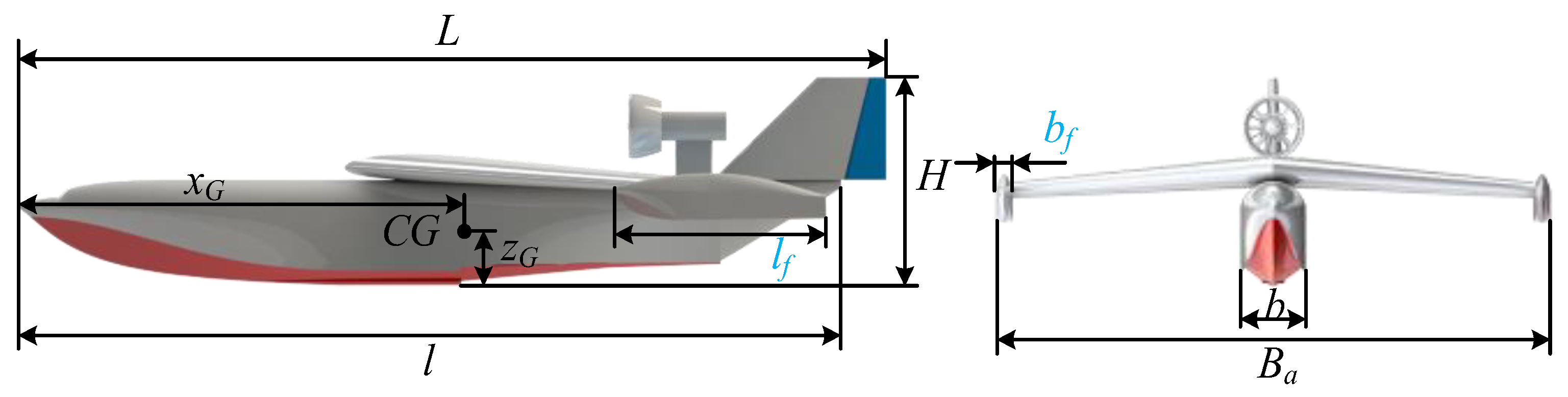
2. The Configuration of the AAMV
3. Motion Model
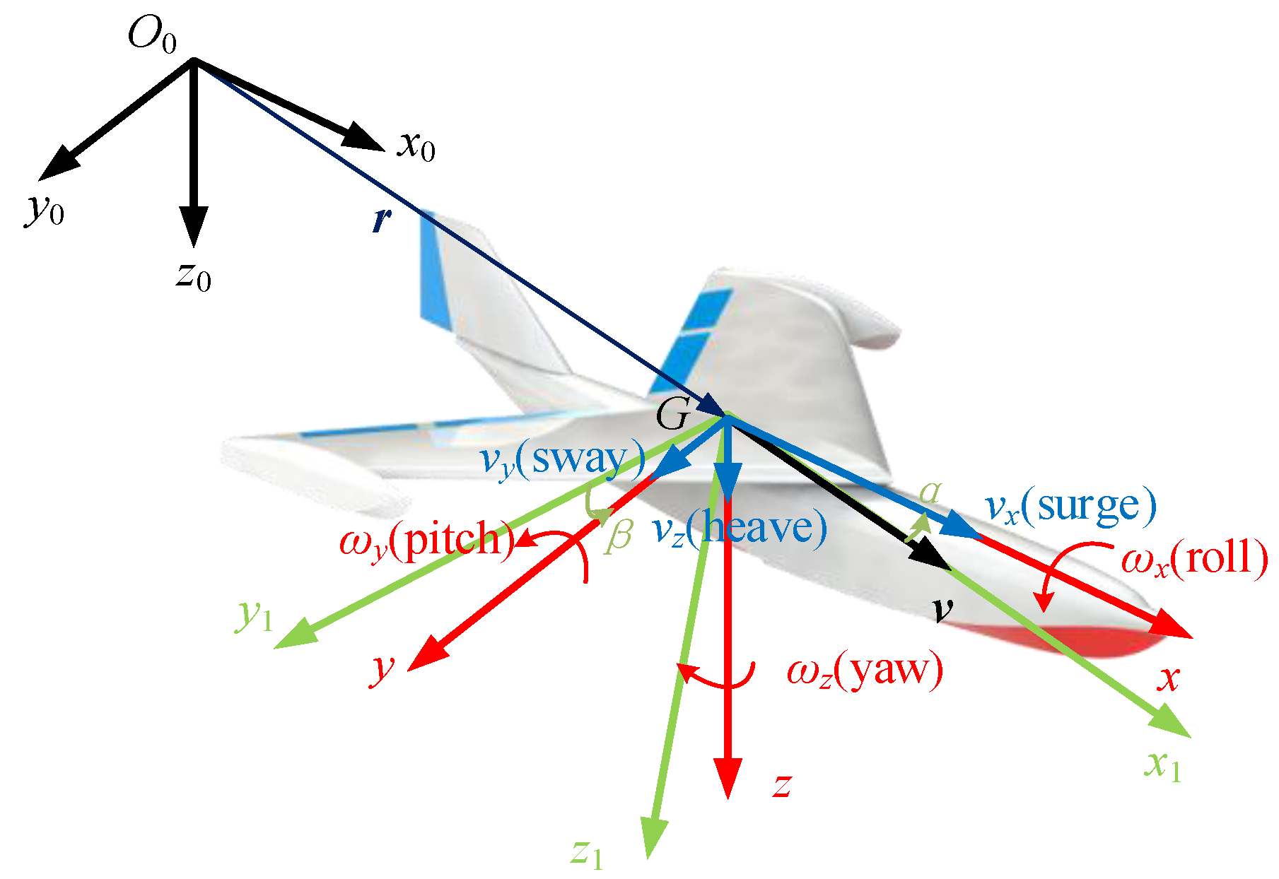
3.1. Coordinate System and Parameter Definition
3.2. Kinematic Model
3.3. Kinetic Model
3.4. Kinetic Analysis
3.4.1. Gravitational Force
3.4.2. Hydrodynamic Force
- (1)
- Buoyancy
- (2)
- Added mass
- (3)
- Viscous forces
3.4.3. Aerodynamic Force
3.4.4. Operating Force
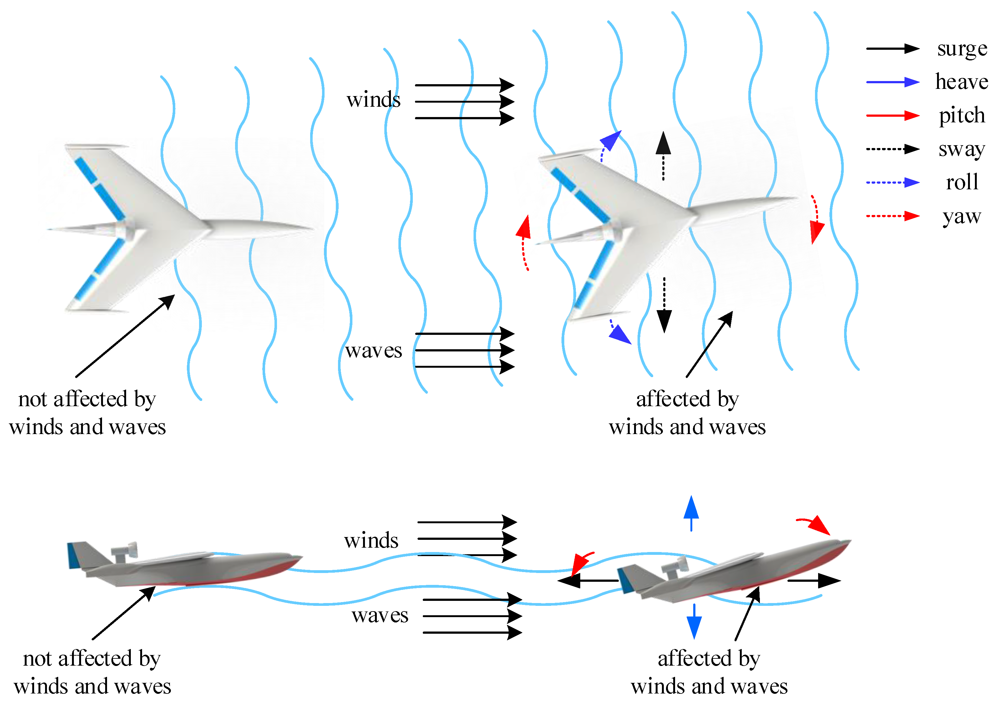
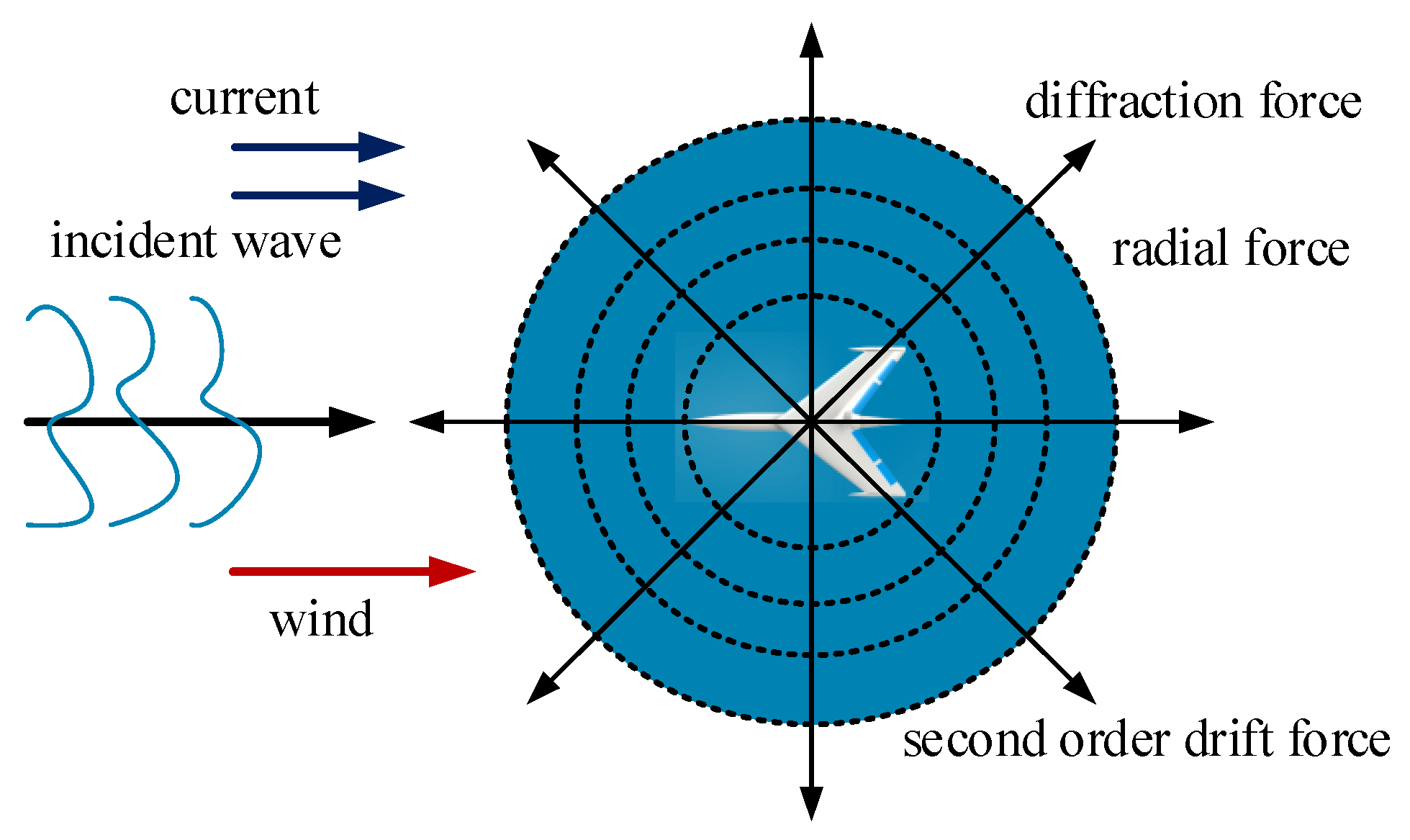
3.4.5. Wind and Wave Disturbance Force
- (1)
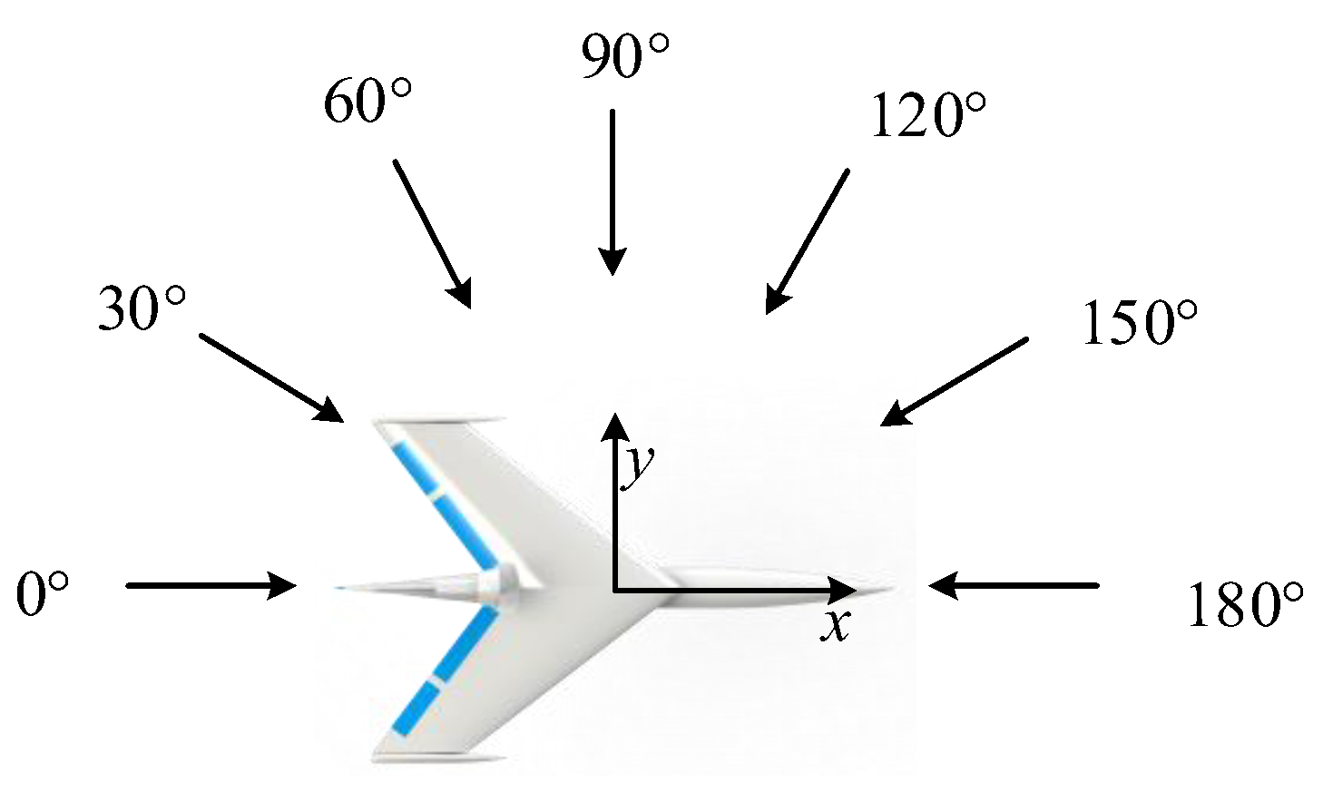
- Force analysis for the problem of the AAMV motion in regular waves
- (2)
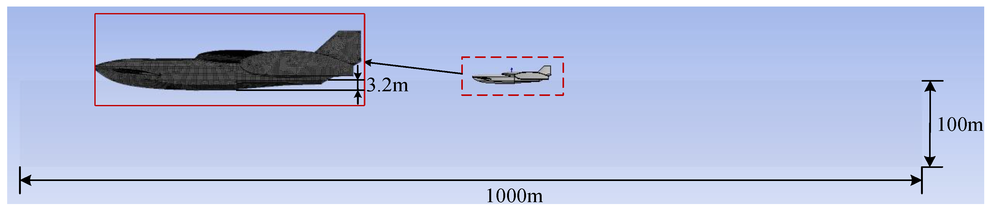
- Numerical model and viscosity correction
- (3)
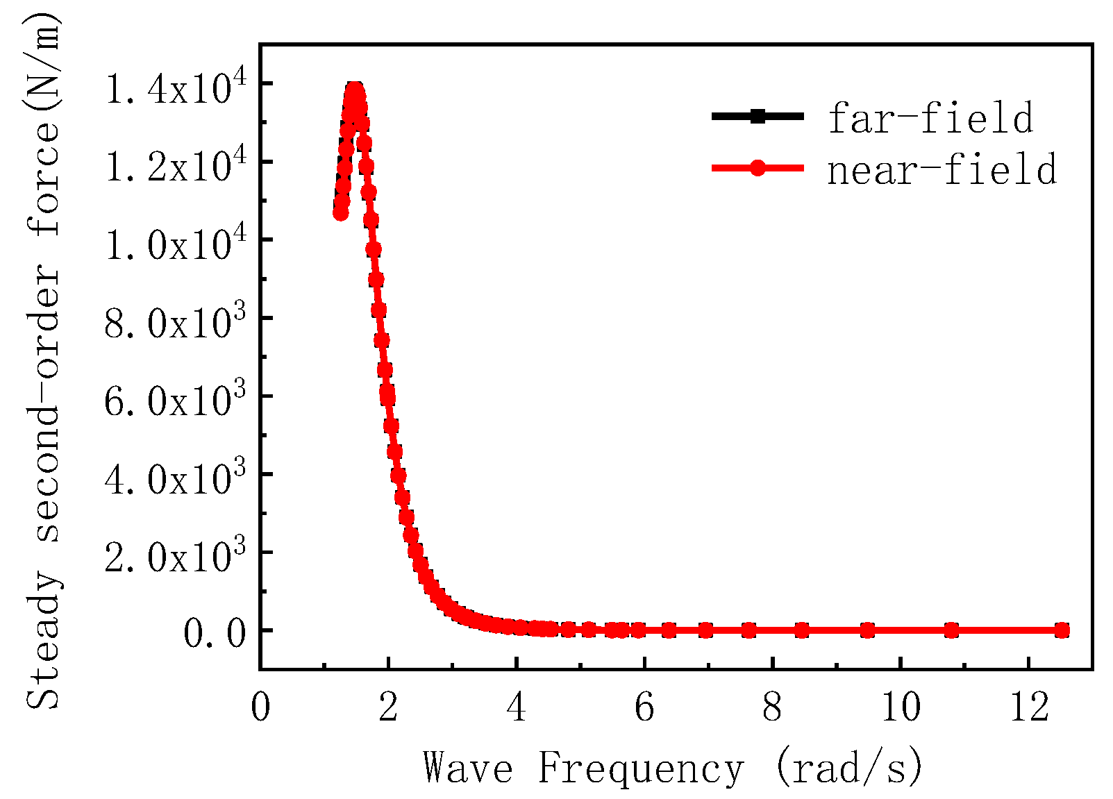
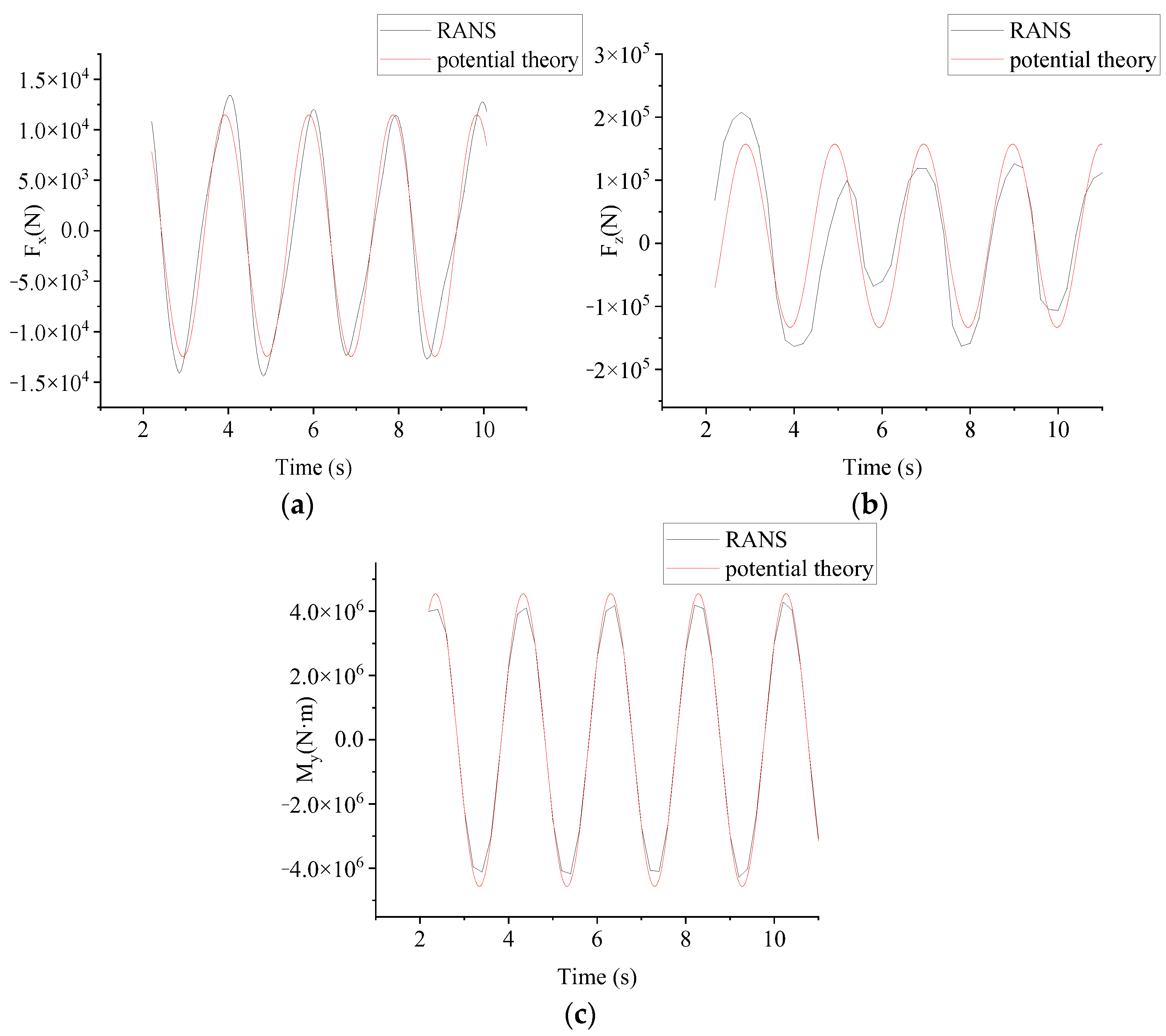
- Verification and validation study
- (4)
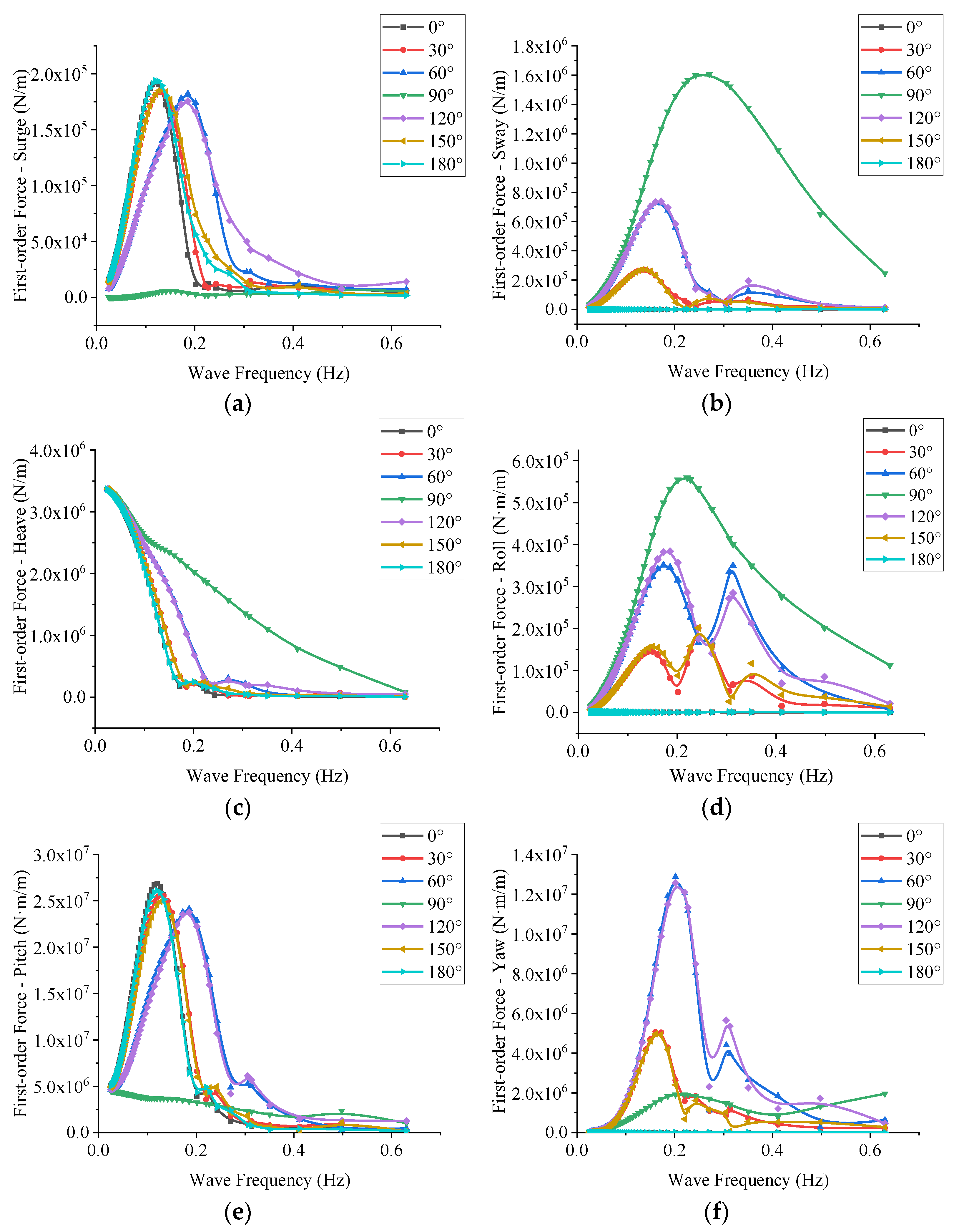
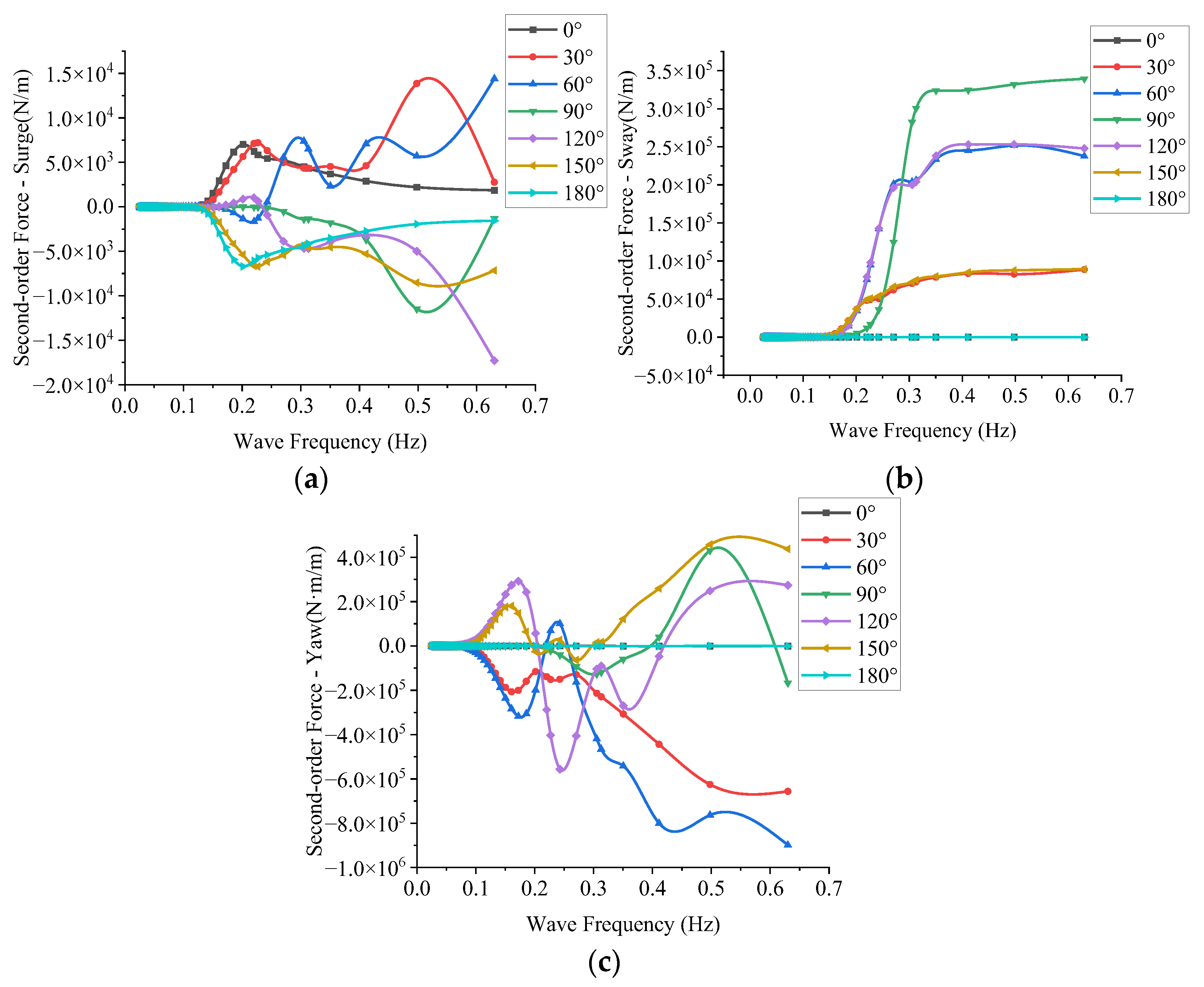
- Numerical results
4. Stability Model
4.1. Longitudinal Stability Model
4.2. Lateral Stability Model
5. Stability Analysis
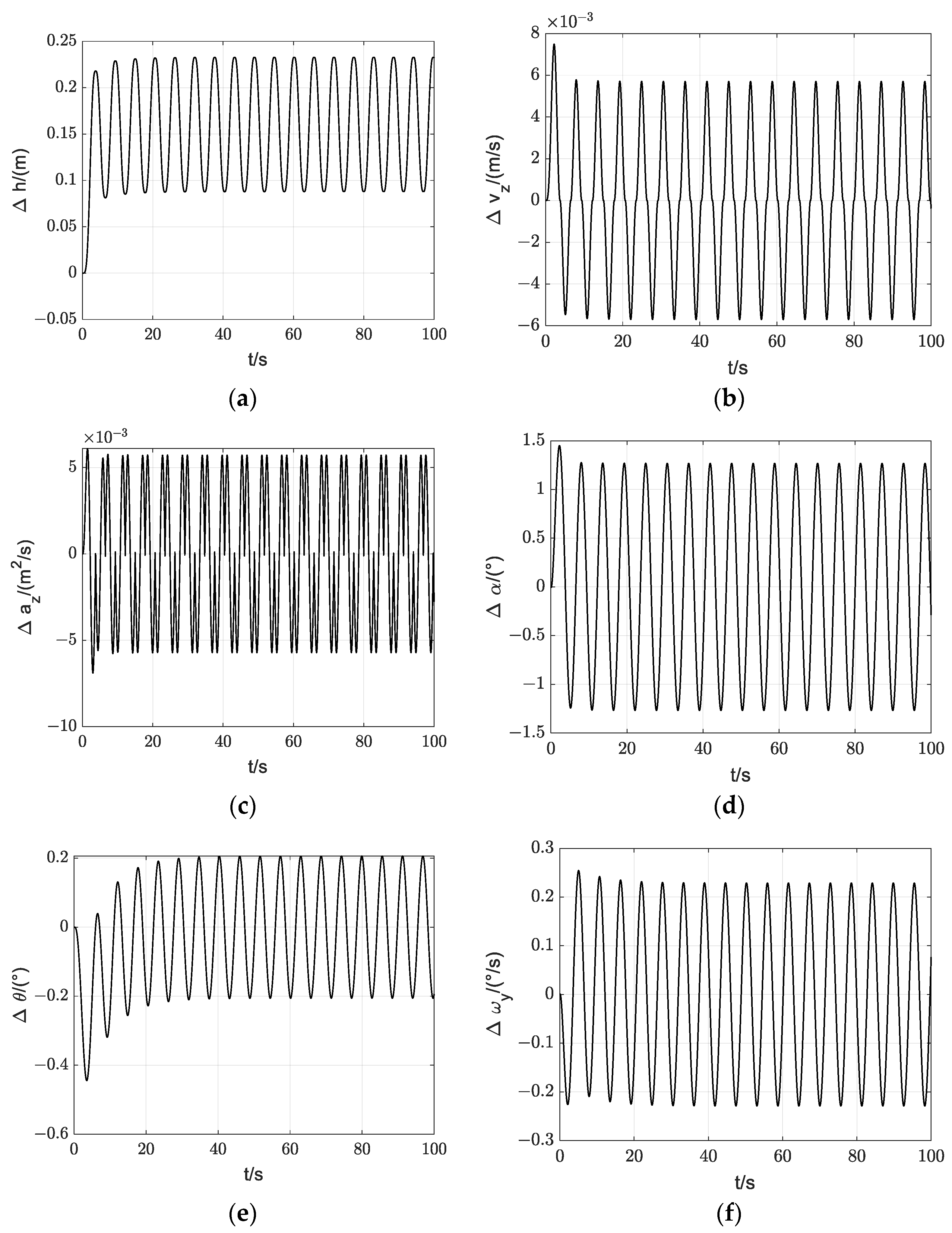
5.1. Longitudinal Stability
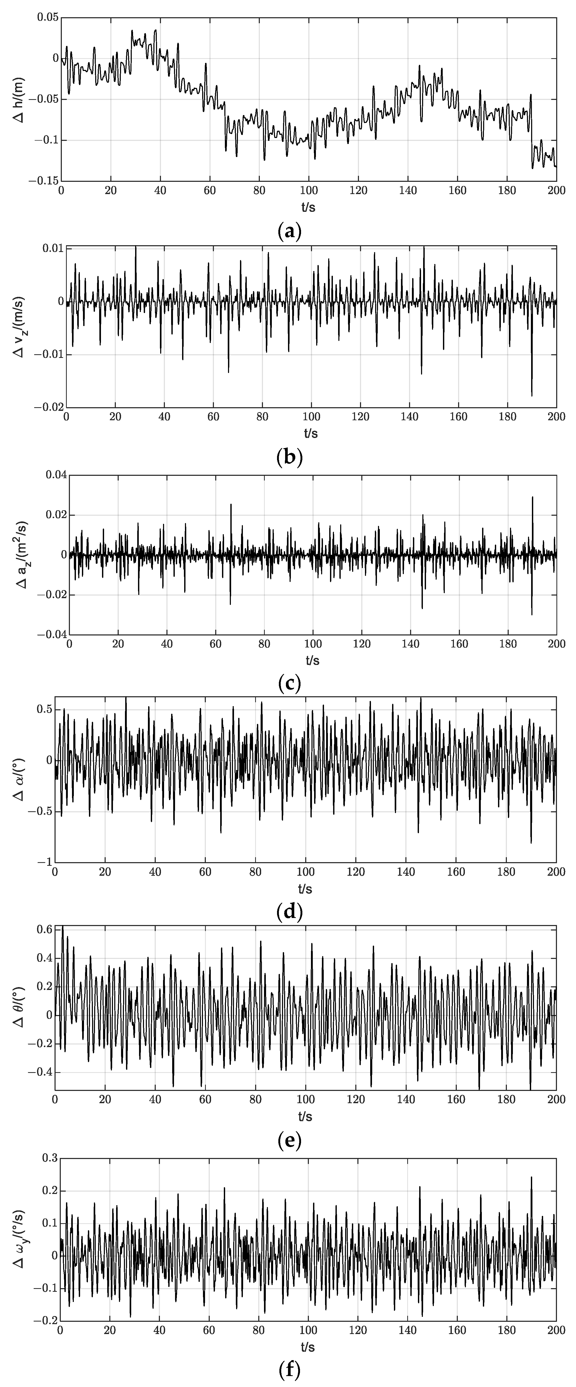
5.2. Lateral Stability
6. Conclusions
Author Contributions
Funding
Institutional Review Board Statement
Informed Consent Statement
Data Availability Statement
Acknowledgments
Conflicts of Interest
References
- Kumar, Y.H.; Vijayakumar, R. Development of an Energy Efficient Stern Flap for Improved EEDI of a Typical High-Speed Displacement Vessel. Def. Sci. J. 2020, 70, 95–102. [Google Scholar] [CrossRef]
- Goldhirsch, I.; Sulem, P.L.; Orszag, S.A. Stability and Lyapunov Stability of Dynamical Systems: A Differential Approach and a Numerical Method. Phys. D Nonlinear Phenom. 1987, 27, 311–337. [Google Scholar] [CrossRef]
- Englar, R.J.; Gregory, S.D.; Ford, D.A. In-Ground-Effect Evaluation and Aerodynamic Development of Advanced Unlimited Racing Hydroplanes. In Proceedings of the 33rd Aerospace Sciences Meeting and Exhibit, Reno, NV, USA, 9–12 January 1995. [Google Scholar] [CrossRef]
- Englar, R.J. Application of Advanced Aerodynamic Technology to Ground and Sport Vehicles. In Proceedings of the 26th AIAA Applied Aerodynamics Conference, Honolulu, HI, USA, 18–21 August 2008. [Google Scholar] [CrossRef]
- Wang, L.; Yang, K.; Yue, T.; Liu, H. Wing-in-Ground Craft Longitudinal Modeling and Simulation Based on a Moving Wavy Ground Test. Aerosp. Sci. Technol. 2022, 126, 107605. [Google Scholar] [CrossRef]
- Zou, J.; Lu, S.; Sun, H.; Zan, L.; Cang, J. Experimental Study on Motion Behavior and Longitudinal Stability Assessment of a Trimaran Planing Hull Model in Calm Water. J. Mar. Sci. Eng. 2021, 9, 164. [Google Scholar] [CrossRef]
- Fossen, T.I. Guidance and Control of Ocean Vehicles; John Wiley & Sons: Hoboken, NJ, USA, 1994; p. 480. [Google Scholar]
- Matveev, K.I. Modeling of Autonomous Hydrofoil Craft Tracking a Moving Target. Unmanned Syst. 2020, 8, 171–178. [Google Scholar] [CrossRef]
- Sahin, O.S.; Kahramanoglu, E.; Cakici, F.; Pesman, E. Control of Dynamic Trim for Planing Vessels with Interceptors in Terms of Comfort and Minimum Drag. Brodogr. Int. J. Nav. Archit. Ocean Eng. Res. Dev. 2023, 74, 1–17. [Google Scholar] [CrossRef]
- Collu, M.; Patel, M.; Trarieux, F. Aerodynamically Alleviated Marine Vehicles (AAMV): Development of a Mathematical Framework to Design High Speed Marine Vehicles with Aerodynamic Surfaces. In Proceedings of the International Conference on High Performance Marine Vehicles 2009 (HPMV09), Shanghai, China, 16–17 April 2009. [Google Scholar]
- Collu, M.; Patel, M.H.; Trarieux, F. The Longitudinal Static Stability of an Aerodynamically Alleviated Marine Vehicle, a Mathematical Model. Proc. R. Soc. Math. Phys. Eng. Sci. 2010, 466, 1055–1075. [Google Scholar] [CrossRef]
- Xu, S.; Chen, K.; Tang, Y.; Xiong, Y.; Ma, T.; Tang, W. Research on the Transverse Stability of an Air Cushion Vehicle Hovering over the Rigid Ground. Ships Offshore Struct. 2022, 17, 2300–2316. [Google Scholar] [CrossRef]
- Vassalos, D.; Xie, N.; Jasionowski, A.; Konovessis, D. Stability and Safety Analysis of the Air-Lifted Catamaran. Ships Offshore Struct. 2008, 3, 91–98. [Google Scholar] [CrossRef]
- Amiri, M.M.; Dakhrabadi, M.T.; Seif, M.S. Development of a Semi-Empirical Method for Hydro-Aerodynamic Performance Evaluation of an AAMV, in Take-off Phase. J. Braz. Soc. Mech. Sci. Eng. 2015, 37, 987–999. [Google Scholar] [CrossRef]
- Amiri, M.M.; Dakhrabadi, M.T.; Seif, M.S. Formulation of a Nonlinear Mathematical Model to Simulate Accelerations of an AAMV in Take-off and Landing Phases. Ships Offshore Struct. 2014, 11, 198–212. [Google Scholar] [CrossRef]
- Song, Y.; Du, X.; Jiang, Y.; Hu, Y. Numerical Investigation on the Resistance Characteristics and Motion Characteristics of the Ultra-High-Speed Aerodynamically Alleviated Marine Vehicle in Regular Head Waves. Ocean Eng. 2023, 289, 116284. [Google Scholar] [CrossRef]
- Aliffrananda, M.H.N.; Sulisetyono, A.; Hermawan, Y.A.; Zubaydi, A. Numerical Analysis of Floatplane Porpoising Instability in Calm Water During Takeoff. Int. J. Technol. 2022, 13, 190–201. [Google Scholar] [CrossRef]
- Mansoori, M.; Fernandes, A.C. The Interceptor Hydrodynamic Analysis for Controlling the Porpoising Instability in High Speed Crafts. Appl. Ocean Res. 2016, 57, 40–51. [Google Scholar] [CrossRef]
- Ding, R.; Zhang, H.; Xu, D.; Liu, C.; Shi, Q.; Liu, J.; Zou, W.; Wu, Y. Experimental and Numerical Study on Motion Instability of Modular Floating Structures. Nonlinear Dyn. 2022, 111, 6239–6259. [Google Scholar] [CrossRef]
- Sukas, O.F.; Kinaci, O.K.; Cakici, F.; Gokce, M.K. Hydrodynamic Assessment of Planing Hulls Using Overset Grids. Appl. Ocean Res. 2017, 65, 35–46. [Google Scholar] [CrossRef]
- De Luca, F.; Mancini, S.; Miranda, S.; Pensa, C. An Extended Verification and Validation Study of CFD Simulations for Planing Hulls. J. Sh. Res. 2016, 60, 101–118. [Google Scholar] [CrossRef]
- Ding, J.; Jiang, J. Tunnel Flow of a Planing Trimaran and Effects on Resistance. Ocean Eng. 2021, 237, 109458. [Google Scholar] [CrossRef]
- Roshan, F.; Dashtimanesh, A.; Bilandi, R.N. Hydrodynamic Characteristics of Tunneled Planing Hulls in Calm Water. Brodogradnja 2020, 71, 19–38. [Google Scholar] [CrossRef]
- Su, G.; Shen, H.; Su, Y. Numerical Prediction of Hydrodynamic Performance of Planing Trimaran with a Wave-Piercing Bow. J. Mar. Sci. Eng. 2020, 8, 897. [Google Scholar] [CrossRef]
- De Marco, A.; Mancini, S.; Miranda, S.; Scognamiglio, R.; Vitiello, L. Experimental and Numerical Hydrodynamic Analysis of a Stepped Planing Hull. Appl. Ocean Res. 2017, 64, 135–154. [Google Scholar] [CrossRef]
- Trimulyono, A.; Luqman, M.; Chairizal, H.; Syaiful, A.; Putra, T.; Tuswan, A.T.; Wibawa, A.; Santosa, B. Analysis of the Double Steps Position Effect on Planing Hull Performances. Brodogr. Int. J. Nav. Archit. Ocean Eng. Res. Dev. 2023, 74, 41–72. [Google Scholar] [CrossRef]
- Samuel, S.; Mursid, O.; Yulianti, S.; Kiryanto; Iqbal, M. Evaluation of interceptor design to reduce drag on planing hull. Brodogr. Int. J. Nav. Archit. Ocean Eng. Res. Dev. 2022, 73, 93–110. [Google Scholar] [CrossRef]
- Kim, Y.; Kim, K.H. Numerical Stability of Rankine Panel Method for Steady Ship Waves. Ships Offshore Struct. 2007, 2, 299–306. [Google Scholar] [CrossRef]
- Pols, A.; Gubesch, E.; Abdussamie, N.; Penesis, I.; Chin, C. Mooring Analysis of a Floating OWC Wave Energy Converter. J. Mar. Sci. Eng. 2021, 9, 228. [Google Scholar] [CrossRef]
- Bonci, M.; De Jong, P.; Van Walree, F.; Renilson, M.R.; Huijsmans, R.H.M. The Steering and Course Keeping Qualities of High-Speed Craft and the Inception of Dynamic Instabilities in the Following Sea. Ocean Eng. 2019, 194, 106636. [Google Scholar] [CrossRef]
- Uharek, S.; Cura-Hochbaum, A. The Influence of Inertial Effects on the Mean Forces and Moments on a Ship Sailing in Oblique Waves Part B: Numerical Prediction Using a RANS Code. Ocean Eng. 2018, 165, 264–276. [Google Scholar] [CrossRef]
- Hashimoto, H.; Yoneda, S.; Omura, T.; Umeda, N.; Matsuda, A.; Stern, F.; Tahara, Y. CFD Prediction of Wave-Induced Forces on Ships Running in Irregular Stern Quartering Seas. Ocean Eng. 2019, 188, 106277. [Google Scholar] [CrossRef]
- Du, X.; Ali, N.; Zhang, L. Numerical Simulations for Predicting Wave Force Effects on Dynamic and Motion Characteristics of Blended Winged-Body Underwater Glider. Ocean Eng. 2021, 235, 109312. [Google Scholar] [CrossRef]
- Faltinsen, O. Sea Loads on Ships and Offshore Structures; Cambridge University Press: Cambridge, UK, 1993. [Google Scholar]
- Fossen, T.I. Handbook of Marine Craft Hydrodynamics and Motion Control; John Wiley & Sons: Hoboken, NJ, USA, 2011. [Google Scholar] [CrossRef]
- John, F. On the Motion of Floating Bodies. I. Commun. Pure Appl. Math. 1949, 2, 13–57. [Google Scholar] [CrossRef]
- ANSYS Inc. Aqwa Theory Manual. Ansys 2015, 15317, 174. [Google Scholar]
- ITTC Resistance Committee ITTC. Uncertainty Analysis in CFD, Validation and Validation Methodology and Procedures, 7.5–03-01–01. ITTC—Recommended Procedures and Guidelines Register. 2017; pp. 1–13. Available online: https://www.ittc.info/media/8153/75-03-01-01.pdf (accessed on 1 July 2024).


| Main Parameters | Notation | Unit | Value | |
|---|---|---|---|---|
| total length | L | m | 92.50 | |
| total width | Ba | m | 56.40 | |
| total height | H | m | 21.30 | |
| mass | m | t | 500.00 | |
| longitudinal center of gravity | xG | m | 36.88 | |
| vertical center of gravity | zG | m | 7.28 | |
| hull | length | l | m | 89.00 |
| width | b | m | 7.00 | |
| float | length | lf | m | 38.00 |
| width | bf | m | 0.90 | |
| Axis | Ground Coordinate System | Body Coordinate System | ||||
|---|---|---|---|---|---|---|
| Description | Translation | Linear Velocity | Description | Rotation | Angular Velocity | |
| x | surge | roll | ||||
| y | sway | pitch | ||||
| z | heave | yaw | ||||
| Sea State | Wind Speed/(m/s) | Significant Wave Height/m | Wavelength/m | Wave Frequency/Hz |
|---|---|---|---|---|
| Class II | 4.37 | 0.366 | 6.10 | 0.505 |
| Class III | 6.95 | 0.884 | 15.85 | 0.313 |
| Class IV | 9.78 | 2.103 | 30.18 | 0.227 |
| Class V | 12.60 | 3.962 | 50.00 | 0.177 |
| Grids | Grid Sizes | Grid Numbers | Surge Wave Loads Fx/N |
|---|---|---|---|
| coarse | 1.1%L | 21,494 | 13,257.4 |
| medium | 0.9%L | 29,059 | 13,262.5 |
| fine | 0.8%L | 38,345 | 13,277.3 |
| Method | Fx/N | Fz/N | My/N·m |
|---|---|---|---|
| RANS | 13,967.7 | 136,892.1 | 4,251,607.9 |
| Potential theory | 13,277.3 | 150,088.3 | 4,468,080.5 |
| Error | 5.2% | 8.7% | 4.8% |
Disclaimer/Publisher’s Note: The statements, opinions and data contained in all publications are solely those of the individual author(s) and contributor(s) and not of MDPI and/or the editor(s). MDPI and/or the editor(s) disclaim responsibility for any injury to people or property resulting from any ideas, methods, instructions or products referred to in the content. |
© 2024 by the authors. Licensee MDPI, Basel, Switzerland. This article is an open access article distributed under the terms and conditions of the Creative Commons Attribution (CC BY) license (https://creativecommons.org/licenses/by/4.0/).
Share and Cite
Song, Y.; Du, X.; Hu, Y. Numerical Study of the Ultra-High-Speed Aerodynamically Alleviated Marine Vehicle Motion Stability in Winds and Waves. J. Mar. Sci. Eng. 2024, 12, 1229. https://doi.org/10.3390/jmse12071229
Song Y, Du X, Hu Y. Numerical Study of the Ultra-High-Speed Aerodynamically Alleviated Marine Vehicle Motion Stability in Winds and Waves. Journal of Marine Science and Engineering. 2024; 12(7):1229. https://doi.org/10.3390/jmse12071229
Chicago/Turabian StyleSong, Yani, Xiaoxu Du, and Yuli Hu. 2024. "Numerical Study of the Ultra-High-Speed Aerodynamically Alleviated Marine Vehicle Motion Stability in Winds and Waves" Journal of Marine Science and Engineering 12, no. 7: 1229. https://doi.org/10.3390/jmse12071229